Towards a unified lattice kinetic scheme for relativistic hydrodynamics

Abstract

We present a systematic derivation of relativistic lattice kinetic equations for finite-mass particles, reaching close to the zero-mass ultra-relativistic regime treated in the previous literature. Starting from an expansion of the Maxwell-Jüttner distribution on orthogonal polynomials, we perform a Gauss-type quadrature procedure and discretize the relativistic Boltzmann equation on space-filling Cartesian lattices. The model is validated through numerical comparison with standard tests and solvers in relativistic fluid dynamics such as Boltzmann approach multiparton scattering (BAMPS) and previous relativistic lattice Boltzmann models. This work provides a significant step towards the formulation of a unified relativistic lattice kinetic scheme, covering both massive and near-massless particles regimes.

I Introduction

Relativistic kinetic theory and relativistic fluid dynamics play an increasingly important role in several fields of modern physics, with applications stretching over widely different scales, ranging from a very rich phenomenology in the realm of astrophysics shore-1992 down to atomic scales (e.g., in the study of the electron properties of graphene in effective 2D systems muller-2008 or the phenomenology of exotic states of quantum matter, such as the recently discovered Weyl fermion pseudo-particles wan-2011 ), further down to subnuclear scales, in the realm of quark-gluon plasmas ackermann-2001 . This motivates the quest for powerful and efficient computational methods, able to accurately study fluid dynamics in the relativistic regime and possibly also to seamlessly bridge the gap between relativistic and low-speed non-relativistic fluid regimes. Over the years, lattice kinetic theory has been at the basis of the development of increasingly complex and accurate lattice Boltzmann methods (LBM), able to simulate many relevant physics problems, including e.g., high Reynolds turbulent regimes, transport in porous media, multi-phase flows and many others succi-2001 ; aidun-2010 ; succi-2015 . One key advantage of most LBM algorithms lies in their computer-friendly structure, that has allowed the development of several massively parallel HPC implementations tolke-2008 ; bernaschi-2009 ; mountrakis-2015 ; calore-2016 .

The last decade has witnessed several attempts to develop LBM capable of handling the relativistic regime. The first model was developed by Mendoza et al. mendoza-2010a ; mendoza-2010b , based on the Grad’s moment matching technique. Romatschke et al. romatschke-2011 developed a scheme for an ultra-relativistic gas based on the expansion on orthogonal polynomials of the Maxwell-Jüttner distribution, following a procedure similar to the one used for non-relativistic LBM. However, this model is not compatible with a Cartesian lattice, thus requiring interpolation to implement the streaming phase. Li et al. li-2012 have extended the work of Mendoza et al. using a multi relaxation-time collision operator, which, by independently tuning shear and bulk viscosity, has allowed the use of a Cartesian lattice. However, this model is not able to recover the third order moments of the distribution. Mohseni et al. mohseni-2013 have shown that it is possible to avoid multi-time relaxation schemes, still using a D3Q19 lattice and properly tuning the bulk viscosity for ultra-relativistic flows, so as to recover only the conservation of the momentum-energy tensor. This is a reasonable approximation in the ultra-relativistic regime, where the first order moment plays a minor role, but leaves open the problem of recovering higher order moments. A further step was taken in mendoza-2013 , with a relativistic lattice Boltzmann method (RLBM) able to recover higher order moments on a Cartesian lattice. This model provides an efficient tool for simulations in the ultra-relativistic regime.

All these developments use pseudo-particles of zero proper mass $m$ (or, more accurately, pseudo-particles for which the ratio particle mass over temperature, $m/T$, goes to zero). This implies that the equation-of-state appropriate for the fluid is the ultra-relativistic one, $\epsilon=3nT$, where $\epsilon$ is the energy density and $n$ the particle density. On the other hand, with the aim of extending the range of physical applications, one would like to explore wider ranges of the $m/T$ ratio and consider mildly relativistic, as well as ultra-relativistic regimes. From the algorithmic point of view, this discussion translates into the aim to develop a unified LBM, with the conceptual and technical ability to bridge the gap between the ultra-relativistic regime ($u/c=\beta\simeq 1$, where $u$ is the fluid speed and $c$ the speed of light), all the way down to the non-relativistic one ($\beta\rightarrow 0$).

This work describes an initial step along this direction, introducing a new RLBM able to cover a wider range of fluid velocities. In the development of the model, we follow a procedure similar to the one used for many non-relativistic LBMs; starting from an expansion of the Maxwell-Jüttner distribution on orthogonal polynomials, we perform a Gauss-type quadrature procedure and discretize the relativistic Boltzmann equation on space-filling Cartesian lattices. We validate this RLBM by comparing with standard tests and solvers in relativistic fluid dynamics and then present a few simulation examples in the direction of prospective applications in astro and subnuclear physics. Realistic applications, as well as hard-core computational aspects, are left for future work.

This paper is structured as follows: In section II, we review the relativistic Boltzmann equation and present an overview of the algorithmic steps involved in the development of our method. In section III, we describe in full detail the procedure used to discretize the relativistic Boltzmann equation on a Cartesian lattice. In section IV, we numerically validate the model against some well-known relativistic flows, while in section V we present preliminary prospects of future physics applications. The paper ends with section VI, summarizing our results and future directions of research. Since the mathematics becomes quickly very involved, many details are moved to appendices, while the most complex mathematical expressions are made available in the form of Supplemental Information supplementary-material .

II Model Description

In this section, we introduce the relativistic Boltzmann equation, and summarize our approach to its discretization in terms of a new RLBM; full details follow in the following section, so a self-contained description of our approach stretches across those two sections.

We consider a single non-degenerate relativistic fluid whose quantum effects are not taken into account. The system is made up of particles with rest mass $m$; in kinetic theory, one is interested in the probability of finding a particle with momentum $\bm{p}$ at a given time $t$ and position $\bm{x}$; we adopt the usual relativistic notation, $x^{\alpha}=\left(ct,\bm{x}\right)$ and $p^{\alpha}=\left(p^{0},\bm{p}\right)$, with $\bm{x}$ and $\bm{p}\in\mathbb{R}^{3}$. The particle distribution function $f(\bm{x},\bm{p},t)=f(x^{\alpha},p^{\beta})$ obeys the relativistic Boltzmann equation that, in the absence of external forces, reads:

$$p^{\alpha}\frac{\partial f}{\partial x^{\alpha}}=\Omega(f)\quad,$$ (1)

with an appropriate collision term $\Omega(f)$. In the non-relativistic regime one usually replaces the collision term with the BGK approximation bhatnagar-1954 ; we adopt the relativistic generalization provided by the Anderson-Witting model anderson-witting-1974a ; anderson-witting-1974b :

$$\Omega(f)=-\frac{U^{\alpha}p_{\alpha}}{\tau_{f}c^{2}}\left(f-f^{eq}\right)\quad,$$ (2)

with $\tau_{f}$ the relaxation (proper-)time, $U^{\alpha}=\gamma\cdot(c,\bm{u})$ ($\gamma=1/\sqrt{1-u^{2}/c^{2}}$) the macroscopic four-velocity, and $f^{eq}$ the local equilibrium distribution, namely the Maxwell-Jüttner distribution:

$$f^{eq}=\frac{1}{\mathcal{N}}\exp{\left(-\frac{p_{\mu}U^{\mu}}{k_{B}T}\right)}\quad;$$ (3)

$\mathcal{N}$ is a normalization constant and $k_{B}$ the Boltzmann constant. In the remainder of this paper we adopt units such that $c=1$, $k_{B}=1$.

Following Grad’s theory grad-1949 the macroscopic description of a relativistic fluid is based on the moments of the distribution function. We consider the first three moments of the distribution, namely the particle four-flow $N^{\alpha}$, the energy-momentum tensor $T^{\alpha\beta}$ and the third-order momentum $T^{\alpha\beta\gamma}$:

$$N^{\alpha} =\int fp^{\alpha}\frac{\mathop{}\!\mathrm{d}\bm{p}}{p_{0}}\quad,$$ (4)

$$T^{\alpha\beta} =\int fp^{\alpha}p^{\beta}\frac{\mathop{}\!\mathrm{d}\bm{p}}{p_{0}}\quad,$$ (5)

$$T^{\alpha\beta\gamma} =\int fp^{\alpha}p^{\beta}p^{\gamma}\frac{\mathop{}\!\mathrm{d}\bm{p}}{p_{0}}\quad.$$ (6)

Hereafter we will use the subscript $E$ to refer to these tensors taken at the equilibrium, i.e. using $f^{eq}$ in place of $f$ in their definition. It can be shown that, see e.g. cercignani-2002 , $N_{E}^{\alpha}$ and $T_{E}^{\alpha\beta}$ are given by

$$N_{E}^{\alpha} =nU^{\alpha}\quad,$$ (7)

$$T_{E}^{\alpha\beta} =\left(\epsilon+P\right)U^{\alpha}U^{\beta}-P\eta^{\alpha\beta};$$ (8)

$n$ is the particle number-density, $\epsilon$ the energy density, $P$ the pressure and $\eta^{\alpha\beta}$ the Minkowski metric tensor (that we write as $\eta^{\alpha\beta}=diag(1,-1,-1,-1))$.

The Anderson-Witting model correctly reproduces the conservation equations:

$$\partial_{\alpha}N^{\alpha} =0\quad,$$ (9)

$$\partial_{\beta}T^{\alpha\beta} =0\quad.$$ (10)

II.1 Discrete relativistic Boltzmann equation

We now describe our approach to derive a relativistic lattice Boltzmann equation, following a procedure similar to the one used with non-relativistic higuera-1989 ; xiaoyi-luo-1997 ; shan-1997 ; martys-1998 and earlier ultra-relativistic LBMs romatschke-2011 ; mendoza-2013 . We perform the following steps:

1. Write Equation 1 in terms of quantities that can be discretized on a regular lattice. Following a standard procedure, we write the explicit expression of the relativistic lattice Boltzmann equation,

   $$p^{0}\partial_{t}f+p^{l}\nabla_{l}f=-\frac{p_{\mu}U^{\mu}}{\tau_{f}}(f-f^{eq})\quad,$$ (11)

   and divide left and right hand sides by $p^{0}$, obtaining:

   $$\partial_{t}f+v^{l}\nabla_{l}f=-\frac{p_{\mu}U^{\mu}}{\tau_{f}p^{0}}(f-f^{eq})\quad,$$ (12)

   with $v^{l}=p^{l}/p^{0}$ the components of the microscopic velocity; in other words, we cast the equation in a form in which the time-derivative and the propagation term are the same as in the non-relativistic regime; the price to pay is an additional dependence on $p^{0}$ of the relaxation term.

2. Expand $f^{eq}$ in an orthogonal basis; we adopt Cartesian coordinates and use a basis of polynomials orthonormal with respect to a weight given by the Maxwell-Jüttner distribution in the fluid rest frame ($\bm{u}=0$):

   $$\omega(p^{0})=\frac{1}{\mathcal{N}_{R}}\exp{\left(-p^{0}/T\right)}.$$ (13)

   where, again, $\mathcal{N}_{R}$ is a normalization factor. Call $\{J^{(i)},i=1,2\dots\}$ these polynomials (that we compute in the following section); then

   $$f^{eq}(\bm{p},U^{\mu},T)=\omega(p^{0})\sum_{k=0}^{\infty}a^{(k)}(U^{\mu},T)J^{(k)}(\bm{p}),$$ (14)

   where the projection coefficients $a^{(k)}$ are

   $$a^{(k)}(U^{\mu},T)=\int f^{eq}(\bm{p},U^{\mu},T)J^{(k)}(\bm{p})\frac{\mathop{}\!\mathrm{d}\bm{p}}{p^{0}}.$$ (15)

   The approximation $f^{Neq}(\bm{p},U^{\mu},T)$, obtained truncating the summation in Equation 14 to the $N$-th order, recovers the same moments as the original distribution function to order $N$, given that the expansion coefficients correspond to the moments of the distribution. For example, a third order expansion ensures that the results of the integrals in Equation 4, 5 and 6 are correctly recovered.

3. Find a Gauss-like quadrature on a regular Cartesian grid able to reproduce correctly the moments of the original distribution up to order $N$. We proceed in such a way as to preserve one of the most important features of lattice Boltzmann models, namely exact streaming; this means that all quadrature points $v^{l}_{i}=p^{l}_{i}/p^{0}$ must sit on lattice sites. At this point, the discrete version of the equilibrium function reads as follows:

   $$f_{i}^{Neq}=w_{i}\sum_{k=0}^{K_{N}}a^{(k)}(U^{\mu},T)J^{(k)}(p^{\mu}_{i})\quad,$$ (16)

   with $w_{i}$ appropriate weights, and $K_{N}$ is the number of orthogonal polynomials up to the order $N$.

4. Use the above result to write the discrete relativistic Boltzmann equation:

   $$f_{i}(\bm{x}+v^{i}\Delta t,t+\Delta t)-f_{i}(\bm{x},t)=-\Delta t~{}\frac{p_{i}^{\mu}U_{\mu}}{p^{0}\tau}(f_{i}-f_{i}^{eq}),$$ (17)

   where $v_{i}$ are the microscopic lattice velocities of each streaming population, and $\tau$ the relaxation time in lattice units (whose relation with $\tau_{f}$ will be discussed in section IV)

Equation 17 allows to simulate the evolution of the system in discrete space and time. Once the $f_{i}$ are known, one computes the energy-momentum tensor (Equation 5) as:

$$T^{\alpha\beta}=\sum_{i}f_{i}p^{\alpha}_{i}p^{\beta}_{i}\quad.$$ (18)

The Anderson-Witting collisional model is only compatible with the Landau-Lifshitz decomposition cercignani-2002 , which implies

$$n= ~{}U_{\alpha}N^{\alpha}\quad,$$ (19)

$$\epsilon U^{\alpha}= ~{}T^{\alpha\beta}U_{\alpha}\quad,$$ (20)

so we obtain the energy density $\epsilon$ and $U_{\alpha}$ solving the eigenvalue problem in Equation 20. Finally temperature is linked to energy and particle density via a suitable equation of state.

Note that Equation 19 and 20 stem from the property of the collision operator to conserve the number of particles and their energy. As a result, its zeroth and first order moments are bound to vanish. Thus, for instance, in the continuum case, right hand side of Equation 11, we calculate the respective moments of the collision operator:

$$-\int\frac{U_{\mu}}{\tau_{f}}(fp^{\mu}-f^{eq}p^{\mu})\frac{\mathop{}\!\mathrm{d}\bm{p}}{p^{0}}\quad=\frac{1}{\tau_{f}}(U_{\mu}N^{\mu}-U_{\mu}N_{E}^{\mu}),$$ (21)

$$-\int\frac{U_{\mu}}{\tau_{f}}(fp^{\mu}p^{\nu}-f^{eq}p^{\mu}p^{\nu})\frac{\mathop{}\!\mathrm{d}\bm{p}}{p^{0}}=\frac{1}{\tau_{f}}(U_{\mu}T^{\mu\nu}-U_{\mu}T_{E}^{\mu\nu})\quad,$$ (22)

and due to the fact that these two expression should be equal to zero, we get

$$U_{\mu}N^{\mu}=U_{\mu}N_{E}^{\mu}\quad,$$ (23)

$$U_{\mu}T^{\mu\nu}=U_{\mu}T_{E}^{\mu\nu}\quad.$$ (24)

Since we know the equilibrium moments, it can be shown that

$$U_{\mu}N^{\mu}=U_{\mu}N_{E}^{\mu}=n\quad,$$ (25)

$$U_{\mu}T^{\mu\nu}=U_{\mu}T_{E}^{\mu\nu}=\epsilon U^{\nu}\quad.$$ (26)

However, it is important to observe that these expressions do not imply that $N^{\mu}=N_{E}^{\mu}$ and $T^{\mu\nu}=T_{E}^{\mu\nu}$, but rather that the non-equilibrium components of $N^{\mu}$ and $T^{\mu\nu}$ are orthogonal to the four-velocity. The same is true in the discrete case, with integrals replaced by summations over the set of discrete velocities.

II.2 Equation of State

As outlined in the introduction, we consider the case of (in-principle) arbitrary values of the particle mass (and hence of the $m/T$ ratio); this allows to consider general equations of state (EOS) not confined to the ultra-relativistic limit;

In the ultra-relativistic regime the EOS is well known:

$$\epsilon=3nT\quad,$$ (27)

A more general EOS for a perfect gas – valid for any value of the $m/T$ ratio – has been derived several decades ago by Karsch et al. karsch-1980 :

$$\epsilon-3nT =(nT)~{}\frac{m}{T}\frac{K_{1}(m/T)}{K_{2}(m/T)}\quad,$$ (28)

$$P =n~{}T\quad;$$ (29)

here and in the following, $K_{i}$ is a modified Bessel function of the second kind of index $i$. Note that $xK_{1}(x)/K_{2}(x)\rightarrow 0$ as $x\rightarrow 0$, so Equation 28 correctly reproduces the ultra-relativistic limit (Equation 27) as $m/T\rightarrow 0$. For the non-relativistic limit, one writes

$$(\epsilon-n~{}m)-3nT=(nT)~{}(\frac{m}{T}\frac{K_{1}(m/T)}{K_{2}(m/T)}-m/T)\quad.$$ (30)

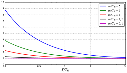
Noting that $(x~{}K_{1}(x)/K_{2}(x)-x)\rightarrow-3/2$ as $x\rightarrow\infty$, and defining $\epsilon_{c}=\epsilon-n~{}m$ (the non-relativistic kinetic energy density), we also recover the well-known non-relativistic expression $\epsilon_{c}=3/2~{}nT$. It is also interesting to look at the difference between Equation 28 and Equation 27 in the intermediate regimes. To this effect, we rearrange Equation 28 in the following way:

$$\frac{\epsilon}{3nT}=1+\frac{1}{3}\frac{m}{T}~{}\frac{K_{1}\left(\frac{m}{T}\right)}{K_{2}\left(\frac{m}{T}\right)},$$ (31)

explicitly highlighting the ratio between the two EOS.

This quantity is plotted in Figure 1 as a function of $T$ for selected values of $m$.

Figure 1: Plot of the RHS of Equation 31 as a function of $T$, for different values of $m$, in arbitrary units.

II.3 Transport Coefficients

The transport coefficients of the model, i.e. shear and bulk viscosities and thermal conductivity, are defined as usual from the non-equilibrium contributions of the energy-momentum tensor cercignani-2002 . The shear viscosity can be obtained by using the following expression,

$$2\eta~{}\partial^{<\alpha}U^{\beta>}=\left(\Delta_{\gamma}^{\alpha}\Delta_{\delta}^{\beta}-\frac{1}{3}\Delta^{\alpha\beta}\Delta_{\gamma\delta}\right)T^{\gamma\delta}\quad,$$ (32)

where $\Delta^{\alpha\beta}\equiv\eta^{\alpha\beta}-U^{\alpha}U^{\beta}$, and the expression $\partial^{<\alpha}U^{\beta>}$ stands for

$$\partial^{<\alpha}U^{\beta>}=\left[\frac{1}{2}\left(\Delta_{\gamma}^{\alpha}\Delta_{\delta}^{\beta}+\Delta_{\delta}^{\alpha}\Delta_{\gamma}^{\beta}\right)-\frac{1}{3}\Delta^{\alpha\beta}\Delta_{\gamma\delta}\right]\partial^{\gamma}U^{\delta}\quad.$$ (33)

The bulk viscosity $\kappa$, on the other hand, can be calculated by using

$$-\kappa~{}\partial_{\alpha}U^{\alpha}=-P-\frac{1}{3}\Delta_{\alpha\beta}T^{\alpha\beta}\quad,$$ (34)

and finally, the thermal conductivity $\lambda$, with the expression

$$\lambda\left(\partial^{\alpha}T-TU^{\beta}\partial_{\beta}U^{\alpha}\right)=\Delta_{\gamma}^{\alpha}U_{\beta}T^{\beta\gamma}\quad.$$ (35)

It is important to mention that, unlike the non-relativistic case, there is no straightforward way to compute the transport coefficients directly from the model parameters, since it is known that the Chapman-Enskog and the Grad procedure deliver (slightly) different results cercignani-2002 . There are also other kind of expansions developed for that purpose israel-1976 ; denicol-2012 and yet an unique expression has not been found. Following Mendoza et al. mendoza-2013 , in this work we shall assume the transport coefficients delivered by the Grad procedure. See later for further discussions on this point.

III Lattice Discretization

In this section we describe in details all steps, outlined in the previous section, required to implement a relativistic lattice Boltzmann procedure, that is, all the ingredients necessary to define and evolve Equation 17.

III.1 Relativistic orthonormal polynomials

We start by constructing an orthonormal basis of polynomials. Following Mendoza et al. mendoza-2013 we adopt the equilibrium distribution in the co-moving frame as our weight function:

$$\omega(p^{0})=\frac{1}{\mathcal{N}_{R}}\exp{\left(-p^{0}/T_{R}\right)}\quad.$$ (36)

Hereafter we will use $T_{R}$ as a normalization factor to write adimensional quantities and to convert from physics to lattice units.

In order to construct a set of orthogonal polynomials we apply the well known Gram-Schmidt procedure, starting from the set $\mathcal{V}=\{1,p^{\alpha},p^{\alpha}p^{\beta},\dots\}$. To carry out this procedure, one must compute integrals of the form

$$I^{\alpha\beta\gamma\dots}=\int\exp{\left(-\frac{p_{\mu}U^{\mu}}{T}\right)}p^{\alpha}p^{\beta}p^{\gamma}\dots\frac{\mathop{}\!\mathrm{d}^{3}p}{p_{0}}\quad,$$ (37)

that can be written in terms of Bessel functionscercignani-2002 . For example:

$$I=\int\exp{\left(-\frac{p_{\mu}U^{\mu}}{T}\right)}\frac{\mathop{}\!\mathrm{d}^{3}p}{p^{0}}=4\pi~{}\frac{m}{T}~{}T^{2}K_{1}\left(\frac{m}{T}\right)\quad,$$ (38)

$$I^{\alpha}=\int\exp{\left(-\frac{p_{\mu}U^{\mu}}{T}\right)}p^{\alpha}\frac{\mathop{}\!\mathrm{d}^{3}p}{p^{0}}=4\pi~{}(\frac{m}{T})^{2}~{}T^{3}K_{2}\left(\frac{m}{T}\right)U^{\alpha};$$ (39)

integrals with higher powers of $p$ are derived by differentiating with respect to $m/T$ and taking into account well-known properties of the Bessel functions.

It is useful to normalize $\omega(p^{0})$ so that

$$\int\omega(p^{0})\frac{\mathop{}\!\mathrm{d}^{3}p}{p_{0}}=1\quad,$$ (40)

implying that

$$\mathcal{N}_{R}=4\pi\frac{m}{T_{R}}T_{R}^{2}K_{1}\left(\frac{m}{T_{R}}\right)=4\pi\bar{m}T_{R}^{2}K_{1}(\bar{m})\quad,$$ (41)

where we adopt the shorthand $\bar{m}=m/T_{R}$.

The complete set of polynomials up to the $2$-nd order has $14$ independent elements while $30$ elements are needed at the $3$-rd order. See Appendix B for all $2$-nd order polynomials, while the complete set (up to $3$-rd order) is available as supplemental material; we label all polynomials as $J^{(n)}_{k_{1}\cdots k_{n}}$, where $n$ is the order of the polynomial and the $k$ indexes corresponds to the components of $p^{\mu}$ they depend upon. As an example, the first non-constant polynomial is

$$J_{0}^{(1)}=\frac{1}{A}\left(\frac{p_{0}}{T_{R}}-\bar{m}\frac{K_{2}(\bar{m})}{K_{1}(\bar{m})}\right)=\frac{1}{A}\left(\bar{p}_{0}-\bar{m}\frac{K_{2}(\bar{m})}{K_{1}(\bar{m})}\right),$$ (42)

All polynomials are adimensional so we write them in terms of $\bar{p}^{\alpha}=p^{\alpha}/T_{R}$; all coefficients, including the normalization constant $A$, only depend on $\bar{m}$.

We now compute $a^{(k)}(U^{\mu},T)$, the projections of $f^{eq}(p,U^{\mu},T)$ (see Equation 15), in a generic reference frame. We choose to normalize $f^{eq}$ so that

$$nU^{\alpha}=N_{E}^{\alpha}=\int f^{eq}p^{\alpha}\frac{\mathop{}\!\mathrm{d}\bm{p}}{p_{0}}\quad,$$ (43)

implying

$$\mathcal{N}=4\pi\left(\frac{m}{T}\right)^{2}T^{3}K_{2}\left(\frac{m}{T}\right).$$ (44)

The computation of these coefficients is a tedious but straightforward task, as it implies again integrals of the form of Equation 37. The coefficients of all polynomials up to the $2$-nd order are listed in Appendix C and all remaining ones are available as supplemental material; coefficient labeling follows the same rules as for polynomials. For example, the explicit expression of $a_{0}^{(1)}$ reads:

$$a_{0}^{(1)} =\int f^{eq}J_{0}^{(1)}\frac{\mathop{}\!\mathrm{d}p^{3}}{p^{0}}$$

$$=\frac{1}{\mathcal{N}}\frac{1}{A}\int\exp{\left(-\frac{p_{\mu}U^{\mu}}{T}\right)}\left[\frac{p_{0}}{T_{R}}-\bar{m}\frac{K_{2}(\bar{m})}{K_{1}(\bar{m})}\right]\frac{\mathop{}\!\mathrm{d}p^{3}}{p^{0}}$$

$$=\frac{1}{T_{R}}\frac{1}{A}\left(U_{0}-\frac{K_{2}(\bar{m})}{K_{1}(\bar{m})}\frac{K_{1}(\frac{m}{T})}{K_{2}(\frac{m}{T})}\right)\quad.$$

All projection coefficients $a^{(k)}$ carry a dimension of one over temperature (or energy); correspondingly, we write them as an explicit $1/T_{R}$ prefactor followed by adimesional expressions written in terms of $m/T_{R}=\bar{m}$ and $m/T$.

III.2 Polynomial expansion of the distribution function at equilibrium

It is now possible to write a polynomial approximation to $f^{eq}$ at any order $N$, via Equation 14, using the explicit expressions for the polynomials and for the expansion coefficients computed in the previous subsections. The analytic expressions quickly become very awkward; for example, the expansion of $f^{eq}$ at first order has $5$ terms and reads:

$$\begin{split}&f^{eq}(p,U,\frac{m}{T_{r}},\frac{m}{T})=\omega(p^{0})\frac{1}{T_{R}}\left(\frac{1}{A^{2}}\left(\bar{p}_{0}-m\frac{K_{2}\left(\bar{m}\right)}{K_{1}\left(\bar{m}\right)}\right)\right.\\ &\left(U_{0}-\frac{K_{1}\left(\frac{m}{T}\right)K_{2}\left(\bar{m}\right)}{K_{2}\left(\frac{m}{T}\right)K_{1}\left(\bar{m}\right)}\right)+\frac{1}{B^{2}}\left(\bar{p}_{x}U_{x}+\bar{p}_{y}U_{y}+\bar{p}_{z}U_{z}\right)\\ &\left.+\frac{K_{1}\left(\frac{m}{T}\right)}{\bar{m}K_{2}\left(\frac{m}{T}\right)}\right)\quad,\end{split}$$ (45)

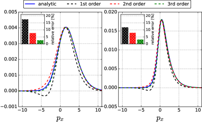
with the coefficients $A$ and $B$ defined in Appendix A. In general, upon factoring out the term $1/T_{R}$, the expression of $f^{eq}$ only depends on the ratios $m/T_{R}=\bar{m}$ and $T/T_{R}$ (in fact we can always write $\frac{m}{T}=\frac{m}{T_{R}}\frac{T_{R}}{T}$). As we will see later, $\bar{m}$ is fixed by the quadrature, while $T/T_{R}$ controls the translation from physical to lattice units. In Figure 2 we compare approximations at the first, second and third order against the analytic Maxwell Jüttner distribution, for several values of $m$, $T$, and $\bm{u}$; as expected, the first order approximation fails to reproduce the analytic behavior, while the second and third order expansions provide increasingly accurate approximations.

Figure 2: Comparison of the analytic Maxwell Jüttner distribution against first, second and third order approximations computed using an orthogonal polynomial basis. Left: $m=5$, $T=1$, $\bm{p}=(p_{x},0,0)$ and $\bm{u}=(0.3,0,0)$; Right: $m=1$, $T=1$, $\bm{p}=(p_{x},0,0)$ and $\bm{u}=(0.4,0,0)$. For each plot, column bars represent the percentage relative L2-error of each approximation with respect to the analytic distribution.

III.3 Quadratures with prescribed abscissa

In order to implement an RLBM on a Cartesian space-filling lattice we need to find the weights and the abscissas of a quadrature satisfying the following orthonormal condition:

$$\begin{split}\int\omega(\bar{p}^{0})J^{(l)}(\bar{p}^{\mu})J^{(k)}(\bar{p}^{\mu})\frac{d^{3}\bar{p}}{\bar{p}^{0}}&=\sum_{n}w_{n}~{}J^{(l)}(\bar{p}^{\mu}_{n})J^{(k)}(\bar{p}^{\mu}_{n})\\ &=\delta_{lk}\quad,\end{split}$$ (46)

where $\{J^{(i)},i=1,2\dots K\}$ are the orthogonal polynomials derived in section III.1, $p^{\mu}_{n}$ are the four-momentum vectors defined at appropriate points in momentum space and the $w_{n}$ are suitable weights philippi-2006 . Our goals is to satisfy the above equation up to the sixth order in $p$, so up to the fifth order of the equilibrium distribution is recovered.

As already discussed, we want to ensure exact streaming, that is we require that all $p^{\mu}_{n}$ sit exactly on sites of our Cartesian grid. We can fulfill this requirement, since we work with a finite value of the particle mass $m$ (hence with a finite value of $m/T_{R}$). To this effect, we adopt populations belonging to several particle groups $G$, each group defining (pseudo-)particles that, at each time step, move from one lattice site to other sites at a given fixed distance. A large list of groups that we can select from is collected in Appendix C. For instance, the well-known non-relativistic D3Q19 model uses the set $\{G_{1},G_{2},G_{3}\}$. Consequently, Equation 46 becomes

$$\begin{split}\int\omega(\bar{p}^{0})J^{(l)}(\bar{p}^{\mu})J^{(k)}(\bar{p}^{\mu})\frac{d^{3}\bar{p}}{\bar{p}^{0}}&=\sum_{i}\sum_{j}w_{j}J^{(l)}(\bar{p}^{\mu}_{i,j})J^{(k)}(\bar{p}^{\mu}_{i,j})\\ &=\delta_{lk}\quad,\end{split}$$ (47)

with $\bar{p}^{\mu}_{i,j}$ corresponding to the $i-$th element of the $j-$th group and $w_{j}$ is the weight of the $j$-th group.

When using more than one group, we ensure exact streaming requiring that velocities of particles belonging to each group are proportional to the (Cartesian-) distance they have to travel to reach their destination. This means that different groups belong to different energy shells. Indeed, we write

$$p^{\mu}_{i,k}=m\gamma_{k}(1,v_{0}\vec{n}_{i,k})\quad.$$ (48)

Here:

• $\vec{n}_{i,k}=(n^{x}_{i,k},n^{y}_{i,k},n^{z}_{i,k})\in\mathbb{N}^{3}$ are the coordinates of the $i-th$ element of the $k-th$ group of the stencil; $||\vec{n}_{k}||$ is the common value of $||\vec{n}_{i,k}||$ for all vectors belonging to group $k$.

• $\gamma_{k}$ is the relativistic $\gamma$ factor associated to $v_{k}=v_{0}~{}||\vec{n}_{k}||$ .

• $v_{0}$ is a common velocity parameter that can be freely chosen under the condition that $v_{k}\leq 1,\forall k$.

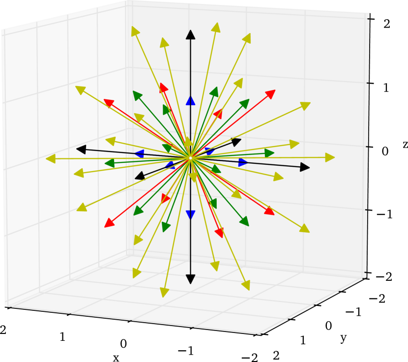
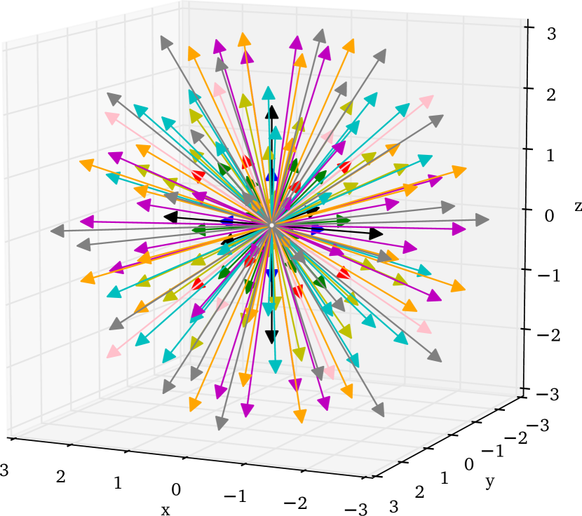
Otherwise stated, the set of the $\vec{n}_{i,k}$ defines the travel path of each element of each group; then, once $v_{0}$ has been set to a specific value, all elements of the group are assigned to an energy shell per Equation 48. Figure 3 shows examples of lattices compatibles with the requirements of Equation 47 and Equation 48.

(a)

(b)

Figure 3: Examples of stencils for the relativistic lattice Boltzmann method. a) Stencil for a second order approximation formed by G = (G1, G2, G3, G4, G5, G6), with $57$ pseudo-populations; b) stencil for a third order approximation formed by G = (G1, G2, G3, G4, G5, G8, G9, G10, G12, G13, G15), with $161$ pseudo-populations.

Assuming that a quadrature has been found and a suitable value for $v_{0}$ has been selected, Equation 17 becomes

$$f_{i}(\vec{x}+v_{0}\vec{n}_{i,k}\delta t,t+\delta t)-f_{i}(\vec{x},t)=-\delta t~{}\frac{p_{i}^{\mu}U_{\mu}}{p^{0}_{i}\tau}(f_{i}-f_{i}^{eq})\quad.$$ (49)

Therefore, our requirement

$$v_{0}\vec{n}_{i,k}\delta t=\vec{N}_{i,k}\delta x\quad,$$ (50)

where $\delta x$ is the lattice spacing and $\vec{N}_{i,k}$ are integer numbers, is equivalent to a relation between time and space units on the lattice.

III.4 Finding quadratures

Assuming for the moment that a certain set of particle groups has been selected, our next step is to find the weights $w_{j}$ of a quadrature that solves Equation 46, that we copy here for convenience, up to a prescribed order:

$$\begin{split}\int\omega(\bar{p}^{0})J^{(l)}(\bar{p}^{\mu})J^{(k)}(\bar{p}^{\mu})\frac{d^{3}\bar{p}}{\bar{p}^{0}}&=\sum_{n}w_{n}~{}J^{(l)}(\bar{p}^{\mu}_{n})J^{(k)}(\bar{p}^{\mu}_{n})\\ &=\delta_{lk}\quad,\end{split}$$ (51)

where $p^{\mu}_{i,k}$ are four-momentum vectors defined in Equation 48. Recall that the values of the $p^{\mu}_{i,k}$ depend on the group to which they belong and on a common hitherto arbitrary value for $v_{0}$.

We follow the procedure described in shan-2010 , building a lattice by adding as many groups as necessary to fulfill Equation 51. For example, considering quadratures giving a second-order approximation, the system of Equation 47 has $6$ linearly independent components , so one needs to build a stencil with (at least) $6$ different groups. Likewise, at third order there are $11$ independent components, so we need $11$ groups. Yet higher order approximations would require stencils with even larger numbers of groups.

Figure 4: Parametric solution of the system of equations given by Equation 47 using the stencil G = (G1, G2, G3, G4, G5, G6) with $\bar{m}=5$. In this case we can identify a region for which $w_{i}(v_{0})\geq 0~{}\forall i$ (orange coloured interval), giving a set of solutions that can be used to build a numerically stable quadrature.

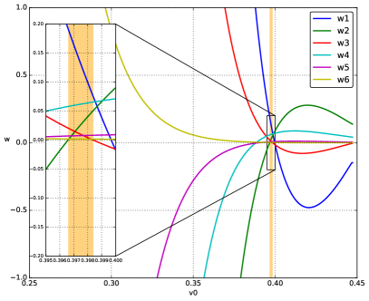
Equation 47 is a linear system in the unknowns $w_{j}$, whose coefficients in principle depend on $m/T_{R}$, on the chosen set of groups and on $v_{0}$. We look for solutions in which $w_{j}\geq 0$ for all $j$s, as this improves numerical stability and is consistent with a (pseudo-)particle interpretation of the RLBM. In practice, one: i) assigns a value for $m/T_{R}$; ii) selects a large enough set of particle groups; and then iii) solves Equation 47 for arbitrary values of $v_{0}$.

Let us see with an example at $2$-nd order the result of this procedure; we take $\bar{m}=5$ and consider the stencil formed by the union of the first six groups in Table 1: G = (G1, G2, G3, G4, G5, G6 ). With this stencil, the longest displacement is given by $G6$ having length $1/\sqrt{5}$, so $v_{0}\in[0,1/\sqrt{5}\approx 0.447)$ as pseudo-particles cannot travel faster than light. Figure 4 shows the values of the $w_{j}$s that solve Equation 51 as a function of $v_{0}$. We see that their values wildly oscillate between large positive and negative values; we can however identify a range of $v_{0}$ values ( $v_{0}\in(0.3966,0.3984)$), for which all weights are positive, providing acceptable solutions to the problem.

Taking for example $v_{0}=0.398$ the corresponding weights for the quadrature are:

$$w_{1}=0.0993921725\dots~{}~{}w_{2}=0.0404025909\dots$$

$$w_{3}=0.0043631818\dots~{}~{}w_{4}=0.0640885469\dots$$

$$w_{5}=0.0081185158\dots~{}~{}w_{6}=0.0018506095\dots$$

Particularly useful values of $v_{0}$ are those located at the boundaries of the interval since, as easily seen in Figure 4, in this case some weights become zero thus pruning certain lattice velocities. In our example one can reduce the set of $57$ velocities to $51$ by setting $w_{2}$ to zero (taking $v_{0}=0.3965826549\dots$), or to $45$ by setting $w_{3}$ to zero ($v_{0}=0.3984063950\dots$). More examples, and accurate values for the weights, are provided in the supplemental material.

In general, many different solutions to the quadrature problem exist. Indeed, one first has the freedom to arbitrarily choose the particle groups (that in turn define the corresponding set of momentum four-vectors per Equation 48) and the reference value for $\bar{m}$ and then one has to pick up a particular value for $v_{0}$. From an algebraic point of view, Equation 51 leads to a linear system of equations, parametric on $v_{0}$:

$$A(v_{0})\bm{w}=\bm{b}\quad.$$ (52)

Here $A$ is a $l\times k$ matrix ($l$ being the number of possible combinations of the orthogonal polynomials, $k$ the number of groups forming the stencil), $\bm{b}$ is a known binary vector, and $\bm{w}$ is the vector of unknowns. Since the Gaussian quadrature requires strictly positive weights in order to guarantee numerical stability, we need to select values of $v_{0}$ (if they exist) such that $w_{i}>0~{}\forall i$. For low-order approximations it is possible to compute an analytic solution, writing each weight $w_{i}$ as an explicit function of the free parameter $v_{0}$, but this become quickly very hard and, already at the second-order, numerical solutions are necessary. A possible formulation of the problem is as follows:

$$\bm{x} =[\bm{w}~{}v_{0}]^{T}\quad$$ , (53)

$$R(\bm{x}) =\|A(v_{0})\bm{w}-\bm{b}\|\quad$$ ,

$$\min_{\bm{x}\in\Re} ~{}\frac{1}{2}R(\bm{x})^{T}R(\bm{x})\quad$$ ,

$$s.t.{} R(\bm{x})=0\quad$$ ,

$$0<v_{0}\leq v_{max}\quad$$ ,

$$w_{i}\geq 0~{}~{}\forall i\quad$$ .

We have performed a detailed exploration of the available phase-space, implementing a solver for Equation 53 based on the LAPACK library with several instances running in parallel on a cluster of CPUs. The solver takes as input a stencil $G$ and tries to find a solution for Equation 53 by scanning several values of $v_{0}$ with a simple steepest-descent method. This fast method allows to scan several stencils at different values of $m/T_{R}$; on the other hand, more robust techniques are desirable in order to perform a more systematic exploration of the phase-space.

Typically, for a given value of $\bar{m}$ several different stencils are possible; however, each stencil works correctly only in a certain range of $\bar{m}$. Still, a reasonably small sets of stencils allows to treat $\bar{m}\geq 0.35$ at the second order and $\bar{m}\geq 1.5$ at the third order, offering a possibility to cover a very large kinematic regime, from almost ultra-relativistic to non-relativistic. A graphical view of (a subset) of all stencils that we have identified, including the corresponding number of populations, is shown in Figure 5 for both $2$-nd and $3$-rd order.

Figure 5: Stencils used to construct a numerically stable quadrature for different value of $\bar{m}$. Top, stencils with six velocity groups, for a second order approximation. Bottom, stencils with eleven velocity vector groups, for a third order approximation. Horizontal bars represent the working range of values $m/T_{R}$ for each quadrature.

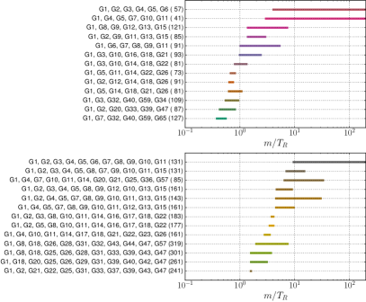
In general, the process of finding working quadratures becomes harder and harder as $\bar{m}$ takes smaller and smaller values. The reason for this, from a strictly mathematical point of view, is that for small values of $\bar{m}$ the condition number of the system matrix in Equation 53 takes large values, therefore requiring more advanced linear algebra techniques. From a physical point of view the reason why this is a difficult problem, and in particular one cannot expect to find solutions for $\bar{m}=0$, is that we require that different groups of particles travel in one time step at different distances hopping from a point of the grid to another point of the grid. In the close to ultra-relativistic regime this requires to restrict to stencils whose elements sit at the intersection between a Cartesian grid and a sphere of given radius. In this case, the trick used by Mendoza et al. mendoza-2013 , of using several energy shells, possible in the ultra-relativistic regime as velocity does not depend on energy, cannot be used if $\bar{m}\neq 0$. Work is in progress to further clarify the best mathematical approach to finding the largest set of available solutions.

We have developed a plain C program that implements our algorithm at second and third order. The code is flexible enough to adapt to any of the possible quadratures and corresponding stencils. The expressions for the polynomials and the equilibrium distribution, obtained using Mathematica software, are almost automatically translated into corresponding C code lines. The overall structure of the code follows the typical implementation of almost all LBM algorithms and shares the same opportunities for massive parallelization. The number of floating point instructions per lattice site for one iteration of the collide kernel, at third order, is 83000 when employing a quadrature with 207 populations; this figure reduces down to 55000 using a 131 point stencil. Note that, consistently with the use of BGK-like collision operator, the instruction count scales approximately linearly with the number of discrete speeds and not quadratically as for the actual Boltzmann collision operator. To put these numbers in perspective, the ultra-relativistic code in mendoza-2013 using a stencil with 128 velocities requires about 52000 instructions; the slight difference can be accounted to the computation of the more complex equation of state and equilibrium function.

IV Numerical Validation

In this section we present a validation of the model by solving the Riemann problem for a quark-gluon plasma. Such a choice is made in order to directly compare against previous RLBM formulations and other relativistic hydrodynamics solvers dealing with the relativistic Boltzmann equation. It should be noted that previous works have focused on the ultra-relativistic regime, which we can only approximate using small values of $m/T_{R}$. As discussed in section III.3 the minimum value of $m/T_{R}$ that can be used in simulations depends on whether we can find a stencil allowing to implement a quadrature for a given value of the rest mass.

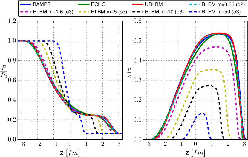
In the following we compare different simulations for the 1D shock-wave problem, showing that decreasing the value of $m/T$ our simulations tends to the results of the ultra-relativistic regime, as computed by well-known codes, such as ECHO-QGP rolando-2014 , the Boltzmann approach multi-parton scattering (BAMPS) xu-greiner-2007 , and the ultra-relativistic RLBM described in mendoza-2013 .

The initial conditions of the simulation, that follow a benchmark performed by BAMPS, are defined by a pressure step having, in physical units, $P_{0}=5.43~{}GeV/fm^{3}$ and $P_{1}=0.339~{}GeV/fm^{3}$, with corresponding initial temperatures $T_{0}=400~{}MeV$ and $T_{1}=200~{}MeV$.

Figure 6: Comparison of the time-evolution of the solution of the Riemann problem obtained with BAMPS (blue lines) and with a second order RLBM solver using $m/T_{R}=0.36$ (green lines). We show the energy (top left), density (top right), pressure (bottom left) and velocity of the shock wave (bottom right), at $t=0~{}fm/c$, $t=1.6~{}fm/c$ and $t=3.2~{}fm/c$. We make use of a $133$ velocities stencil given by G = G1, G14, G49, G51, G60, G70.

Figure 7: Pressure and velocity profiles (at $t=3.2~{}fm/c$) of the same 1D Riemann problem of Figure 6, obtained via a 2D simulation. Results agree with those of the 1D simulation to machine precision.

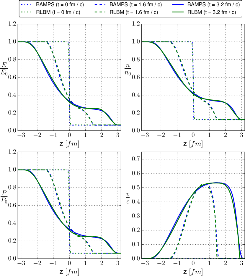
To make contact with real-life physics, it is necessary to convert from physical units to lattice units. In our simulations we set the following values for the initial temperature $T_{0}=1$, $T_{1}=0.5$ (this means that we set the scale of our reference temperature $T_{R}=400~{}MeV$), and the values $n_{0}=1$, $n_{1}=0.124$ for the initial density, which correctly reproduce the ratio $P_{1}/P_{0}$. To relate physical space and time units with the corresponding lattice units, one starts by assigning the physical length $\delta x$ corresponding to one lattice spacing; one arbitrary population group in the simulation stencil, having velocity $||n_{k}||v_{0}$, travels a distance of $||n_{k}||$ lattice spacings in one time unit; then, if we call $dt$ the physical time unit corresponding to one discrete time step, $||n_{k}||v_{0}\delta t=||n_{k}||\delta x$, so we finally obtain $\delta t=\delta x/v_{0}$.

Another quantity that one must properly scale in order to use consistently different quadratures is the relaxation time $\tau$. In the numerical setup $\tau$ is expressed in lattice time units, so it naturally follows from the discussion on the discrete time steps $\delta t$ that $\tau$ can be written as $\tau=\tau_{f}v_{0}/\delta x$, and $\tau_{f}$ is related to the transport coefficients of the system that one wants to study.

Figure 8: Comparison of the time-evolution of the Riemann problem obtained with a RLBM solver using different quadratures, at the second and third order $(m/T_{R}=5)$. Quadrature A ($2$-nd order): G = G1, G4, G5, G7, G10, G11. $v_{0}=0.2600738$. Quadrature B ($2$-nd order): G = G1, G2, G3, G4, G5, G6. $v_{0}=0.3609900$. Quadrature C ($3$-nd order): G = G1, G2, G3, G4, G6, G7, G9, G10, G11, G13, G15. $v_{0}=0.2722674$. Quadrature D ($3$-nd order): G = G1, G8, G18, G26, G28, G31, G32, G43, G44, G47, G57. $v_{0}=0.1571087$.

The accurate link between the transport coefficients and $\tau_{f}$ in the relativistic regime is still debated in the literature. The approaches based on Grad’s method of moments and on the Chapman-Enskog theory give slightly diverging results in the relativistic regime (even if they agree in the non-relativistic limit), see cercignani-2002 . Attempts to clarify this situation have been made by Israel and Stewart israel-1976 and more recently in a series of papers by Denicol et al. denicol-2012 ; molnar-2014 . In our tests, we use Grad’s method (also adopted in mendoza-2013 ), expecting only limited inaccuracies, of the order of $\simeq 10-15\%$. Therefore, at this stage we are not including contributions from massive particles in the transport coefficients, thus relating the relaxation time $\tau$ to the shear viscosity $\eta$ through $\eta=(2/3)P(\tau-\delta t/2)$; work is in progress in order to improve and generalize this definition for our RLBM formulation.

Figure 9: Relative L2-distance of our simulated solution at second order (left) and third order (right) with respect to BAMPS and with respect to the ultra-relativistic LBM (URLB), as a function of the $m/T_{R}$ ratio; we see that solutions become closer and closer as the $m/T_{R}$ ratio becomes smaller. Each point is obtained making use of the stencil having the smallest number of velocities.

We perform our first tests on a lattice with $1\times 1\times 6400$ cells, half of which represents our domain defined in the interval $(-3.2~{}fm,3.2~{}fm)$, and the other half forming a mirror which allows us to use periodic boundary conditions. It follows that on our grid $6.4~{}fm$ corresponds to $3200$ grid points, that is $\delta x=0.002~{}fm$; the value of $\delta t$ for any given quadrature can be derived as explained in the previous paragraph. Figure 6 shows a typical result of this test, where we compare the energy, density, velocity and pressure profiles of BAMPS with $\eta/s=0.1$ against our model. Here $s$ is the entropy density, calculated according to the relation $s=4n-n\ln{(n/n^{eq})}$, where $n^{eq}$ comes from the equilibrium function, $n^{eq}=d_{G}T^{3}/\pi^{2}$, with $d_{G}=16$ the degeneracy of the gluons. The profiles show the evolution of the system from $t=0~{}fm/c$ to $t=3.2~{}fm/c$; Figure 6 shows that the results obtained simulating for $m/T_{R}=0.36$ are in very good agreement with BAMPS; one may relate this nice and (possibly) unexpected behavior to the mild differences between the EOS of the two systems in this regime (see again Figure 1).

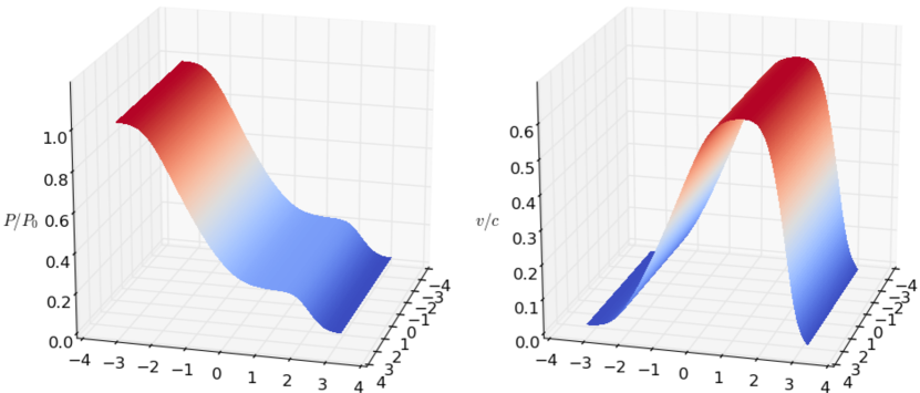
Although for validation purposes we consider only one dimensional simulations, our model readily extends to two and three spatial dimensions. Figure 7 shows a 2D example where we solve the same Riemann problem on a 2D grid of $1\times 800\times 800$ sites; we have checked that 1D and 2D results agree almost to machine precision.

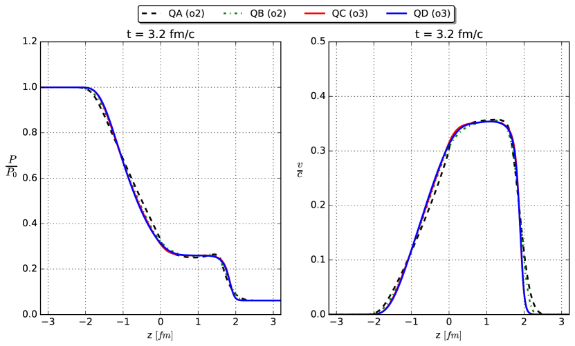
A further validation of our model is offered by the consistency among simulations of the same physical setup, performed with different quadratures. In principle one expects the same results, after appropriately rescaling the space and time units as discussed above; in practice, small differences may appear, as different quadratures provide slightly different approximations to the distribution moments.

This is shown in Figure 8, where we compare results obtained by simulating the same problem with different quadratures at the 2nd and 3rd order. We see a close to perfect agreement at third order. On the other hand, as one would expect, the results are slightly divergent when using second order quadratures since the moments related to the viscosity terms are not fully recovered and different quadratures introduce different errors in their approximation.

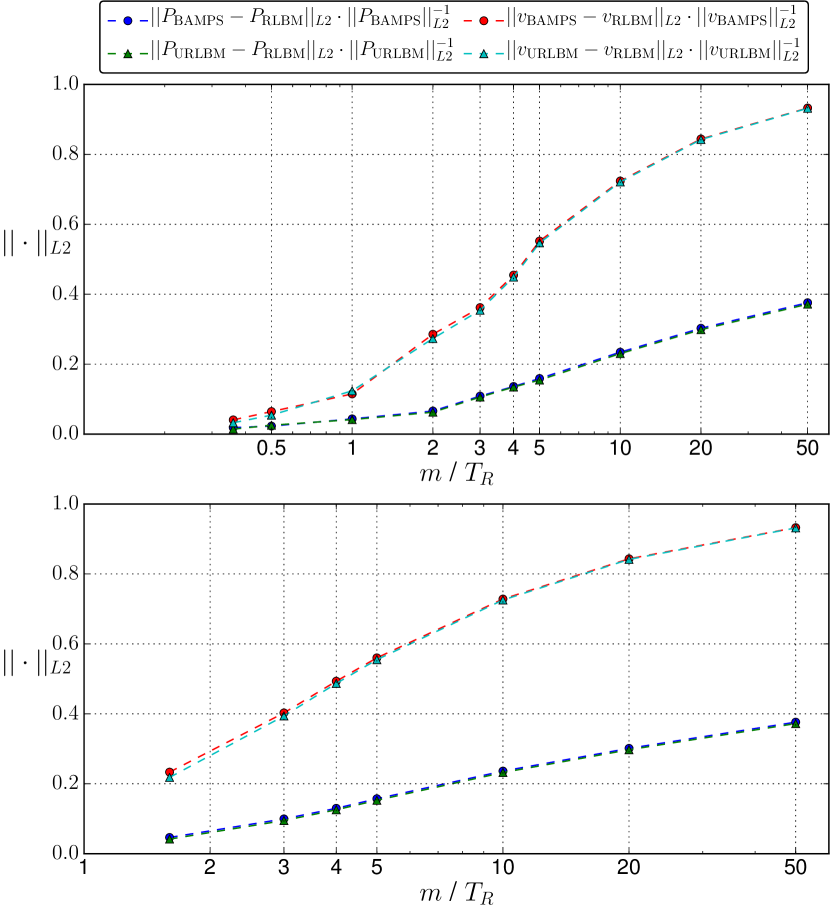
We conclude this section with a more general validation test, presented in Figure 9, where we show that our solutions becomes closer and closer to the ultra-relativistic ones, as we reduce the $m/T$ ratio; this shows that the present algorithm is a good candidate to bridge the gap between ultra-relativistic and non-relativistic regimes.

V Results and prospective applications

The RLBM scheme presented in this paper allows to explore many different physics regimes, from a nearly ultra-relativistic behavior, down to mildly relativistic ones. While we leave physics applications to future works, here we wish to offer just a few preliminary examples, conveying a sense of prospective physics applications of the present method.

In Figure 10 we show the behavior of a fluid undergoing a Riemann-like shock, for a fixed value of $\eta/s$, and for different values of $m/T$ placing ourselves at different relativistic regimes. One easily appreciates the changes in the system evolution as one moves from a strongly relativistic to an almost classic regime: the evolution from the same initial temperature and pressure gradients becomes slower as $m/T$ becomes larger.

We conclude by testing the stability of our algorithm when considering fully two-dimensional simulations. Once again, the reader should be aware that the aim here is not a detailed study of a real physical application but rather to give a taste of what the model allows to do. We also like to point out that while the examples presented in the following have been performed also in three dimensions, we report here only two dimensional profiles for the sake of visualization.

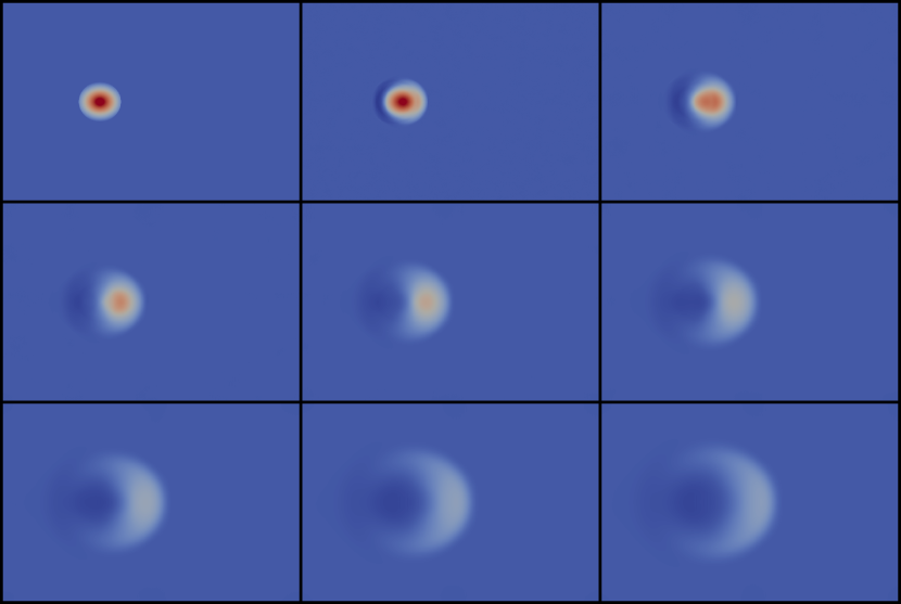
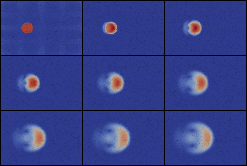
In Figure 11 we present a relativistic analogue of the Taylor-dispersion process taylor-1953 , simulating the dynamics of a circular domain of radius $R$ with an initial radial density $n(r)=n_{0}(1-r/R)$, and an initial velocity $v=(\frac{c}{2},0)$. 11(a) outlines the density profile of the system at eight different time steps, while in parallel 11(b) shows the evolution of the velocity magnitude; the pictures show a substantial mixing of the fast moving fluid with the environment, qualitatively similar to the one exhibited by its low-speed analogue.

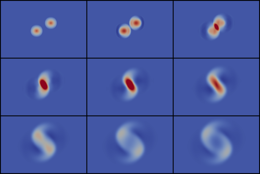
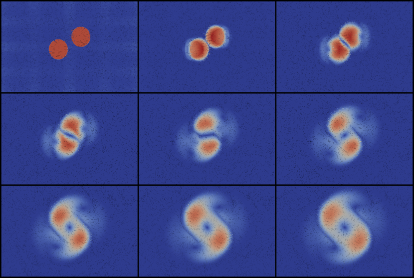
The simulation presented in Figure 12 points in the direction of quark-gluon plasma phenomenology, as we consider two domains with the same initial density as before, traveling in opposite directions at speed $v\sim\frac{c}{2}$. The pressure profile (12(a)), and the velocity magnitude (12(b)) are shown at eight different time steps.

In order to apply our model to realistic simulations in quark-gluon plasma one would need to consider further extensions, as for instance suitable EOS and appropriate initial and boundary conditions. Still, the picture capture features of an hydrodynamic evolution of fluid following the initial collision among nuclei, as long as the temperature remains larger than the freeze-out threshold cooper-1974 . Our simulation method might also permit to apply the fluid-dynamic approach across the deconfinement transition point, in the very interesting region where the fluid speed of “sound” ($c^{2}_{s}=\partial p/\partial\epsilon$) changes abruptly (decreasing down to the so-called “softest point” and then increasing again) and in which the role of the hadronic degrees of freedom will start to play a significant dynamic role heinz-2005 ,chojnacki-2005 . We expect the range $1<m/T<5$ to be relevant in this case, as they correspond to the ratio of the mass of the low-lying hadrons (e.g. pion, $\rho$-meson, nucleon) to the deconfinement temperature.

Figure 10: Comparison of different relativistic hydrodynamics solvers. Dashed lines represent the results obtained using our RLBM solver implementing a second and a third order approximation for different values of $\bar{m}$. Left) Pressure profile at $t=3.2~{}fm/c$. Right) Velocity profile at $t=3.2~{}fm/c$.

VI Conclusions and Outlook

In this paper we have developed a new class of relativistic lattice Boltzmann methods, that provides a wider degree of generality and flexibility with respect to previous models, while still preserving all features of conceptual simplicity and computational efficiency of lattice Boltzmann methods. The main results of this work are summarized as follows:

• We have explicitly built a new class of RLBM based on massive pseudo-particles, able to recover the moments of the relativistic equilibrium distribution up to third order.

• The use of massive pseudo-particles translates into the possibility to tailor the detailed features of the method to fit a specific relativistic range of velocities of the simulated system, ranging from strongly relativistic to almost classical.

• We have established a methodology capable of quickly deriving many different variants of the present RLBM, allowing for instance to use different sets of pseudo-particles and to adjust the value of $m/T$.

• The algorithmic structure of the present RLBM is very similar to that of other established lattice Boltzmann methods and the computational complexity is not much higher. This algorithm retains the same computational advantages, offering high amenability to parallelization, that can be exploited to write efficient high-performance computing codes.

• Initial tests have shown that our algorithms are computationally stable and robust over a wide range of physical parameters.

(a) Density

(b) Velocity

Figure 11: Evolution of a Lorentz contracted circular domains with a radial initial density moving with a initial velocity $v=0.5~{}c$. Starting from $t=0$ we present 9 frames, taken at $6$ time steps apart, showing profiles of: a) Particle density. b) Velocity magnitude.

To the best of our knowledge, this is the first RLBM implementing exact streaming on a Cartesian lattice without losing spatial resolution and still recovering higher order moments of the equilibrium distribution. The flexibility of this RLBM should make it an appealing computational tool to study several relevant relativistic physics problems, including for instance astrophysical contexts shore-1992 or quark-gluon plasma dynamics ackermann-2001 , or the transport properties of electronic pseudo-particles in 2D or 3D solid-state systems muller-2008 ; wan-2011 .

(a) Pressure

(b) Velocity

Figure 12: Evolution of the collision between two Lorentz contracted circular domains with a radial initial density moving with a initial velocity $v=0.5~{}c$. Starting from $t=0$ we present 9 frames, taken at $6$ time steps apart, showing profiles of: a) Pressure. b) Velocity magnitude.

From the algorithmic point of view, we plan to work on further optimizations of the method, by studying for instance the physics accuracy and the computational efficiency of different stencil options. We also plan to look at the low-velocity limit of our algorithms, with the goal of fully bridging the gap between relativistic and non-relativistic LBMs. Work along these lines is in progress.

Appendix A Second-order Relativistic Orthonormal Polynomials

This and the following appendix sections provide several mathematical details relevant in our calculations. As mathematical complexity quickly becomes very large, many very complex expressions are available as supplemental information supplementary-material . In this section we provide the analytic expressions of the orthonormal polynomials, up to the second order, as a function of $\bar{p}^{\mu}=p^{\mu}/T_{R}$.

$$J^{(0)} =1$$

$$J^{(1)}_{0} =\frac{1}{A}\left(\bar{p}_{0}-\frac{\bar{m}K_{2}(\bar{m})}{K_{1}(\bar{m})}\right)$$

$$J^{(1)}_{x} =\frac{1}{B}\bar{p}_{x}$$

$$J^{(1)}_{y} =\frac{1}{B}\bar{p}_{y}$$

$$J^{(1)}_{z} =\frac{1}{B}\bar{p}_{z}$$

$$J^{(2)}_{00} =\frac{1}{\sqrt{3}\ C}\left(\bar{p}_{0}^{2}+\bar{p}_{0}\left(\frac{3}{-\frac{\bar{m}K_{1}(\bar{m})}{K_{2}(\bar{m})}+\frac{\bar{m}K_{2}(\bar{m})}{K_{1}(\bar{m})}-3}-3\right)+\frac{3K_{1}(\bar{m})(\bar{m}K_{1}(\bar{m})+3K_{2}(\bar{m}))}{\bar{m}K_{1}(\bar{m}){}^{2}+3K_{2}(\bar{m})K_{1}(\bar{m})-\bar{m}K_{2}(\bar{m}){}^{2}}-\bar{m}^{2}-3\right)$$

$$J^{(2)}_{0x} =\frac{1}{D}\bar{p}_{x}\left(\bar{p}_{0}-\frac{\bar{m}K_{3}(\bar{m})}{K_{2}(\bar{m})}\right)$$

$$J^{(2)}_{0y} =\frac{1}{D}\bar{p}_{y}\left(\bar{p}_{0}-\frac{\bar{m}K_{3}(\bar{m})}{K_{2}(\bar{m})}\right)$$

$$J^{(2)}_{0z} =\frac{1}{D}\bar{p}_{z}\left(\bar{p}_{0}-\frac{\bar{m}K_{3}(\bar{m})}{K_{2}(\bar{m})}\right)$$

$$J^{(2)}_{xx} =\frac{1}{E}\left(\frac{\bar{p}_{y}^{2}}{2}-\frac{\bar{p}_{z}^{2}}{2}\right)$$

$$J^{(2)}_{yy} =\frac{1}{2\sqrt{3}E}\left(-2\bar{p}_{x}^{2}+\bar{p}_{y}^{2}+\bar{p}_{z}^{2}\right)$$

$$J^{(2)}_{xz} =\frac{1}{E}\bar{p}_{x}\bar{p}_{z}$$

$$J^{(2)}_{yz} =\frac{1}{E}\bar{p}_{y}\bar{p}_{z}$$

$$J^{(2)}_{xy} =\frac{1}{E}\bar{p}_{x}\bar{p}_{y}$$

with:

$$A =\sqrt{\bar{m}\left(\bar{m}+\frac{K_{2}(\bar{m})(3K_{1}(\bar{m})-\bar{m}K_{2}(\bar{m}))}{K_{1}(\bar{m}){}^{2}}\right)}$$

$$B =\sqrt{\frac{\bar{m}K_{2}(\bar{m})}{K_{1}(\bar{m})}}$$

$$C =\sqrt{2\bar{m}^{2}+\frac{5\bar{m}K_{2}(\bar{m})}{K_{1}(\bar{m})}-\frac{3K_{1}(\bar{m})(\bar{m}K_{1}(\bar{m})+3K_{2}(\bar{m}))}{\bar{m}K_{1}(\bar{m}){}^{2}+3K_{2}(\bar{m})K_{1}(\bar{m})-\bar{m}K_{2}(\bar{m}){}^{2}}+3}$$

$$D =\sqrt{\frac{\bar{m}^{2}\left(\bar{m}K_{2}(\bar{m}){}^{2}+5K_{3}(\bar{m})K_{2}(\bar{m})-\bar{m}K_{3}(\bar{m}){}^{2}\right)}{K_{1}(\bar{m})K_{2}(\bar{m})}}$$

$$E =\sqrt{\frac{\bar{m}^{2}K_{3}(\bar{m})}{K_{1}(\bar{m})}}$$

Appendix B Second-order Orthogonal Projections

In this appendix we will provide the analytic expressions of the orthogonal projections $a^{(k)}$, up to the second order, written as

$$a^{(k)}=\frac{1}{T_{R}}b^{(k)}$$

$$b^{(0)} =\frac{1}{\bar{m}}\frac{K_{1}(\frac{m}{T})}{K_{2}(\frac{m}{T})}$$

$$b^{(1)}_{0} =\frac{1}{A}\left(U_{0}-\frac{K_{2}(\bar{m})}{K_{1}(\bar{m})}\frac{K_{1}(\frac{m}{T})}{K_{2}(\frac{m}{T})}\right)$$

$$b^{(1)}_{x} =\frac{1}{B}U_{x}$$

$$b^{(1)}_{y} =\frac{1}{B}U_{y}$$

$$b^{(1)}_{z} =\frac{1}{B}U_{z}$$

$$b^{(2)}_{00} =\frac{1}{\sqrt{3}C}\left(U_{0}^{2}\left(\bar{m}\frac{K_{3}(\frac{m}{T})}{K_{2}(\frac{m}{T})}\right)+U_{0}\left(\frac{1}{-\frac{\bar{m}K_{1}(\bar{m})}{K_{2}(\bar{m})}+\frac{\bar{m}K_{2}(\bar{m})}{K_{1}(\bar{m})}-3}-1\right)\right.$$

$$\left.+\frac{K_{1}(\frac{m}{T})}{K_{2}(\frac{m}{T})}\left(\frac{-\bar{m}^{2}K_{1}(\bar{m})^{2}+\left(\bar{m}^{2}+3\right)K_{2}(\bar{m})^{2}-3\bar{m}K_{2}(\bar{m})K_{1}(\bar{m})}{\bar{m}K_{1}(\bar{m})^{2}+3K_{2}(\bar{m})K_{1}(\bar{m})-\bar{m}K_{2}(\bar{m})^{2}}+\frac{T}{T_{R}}\frac{K_{2}(\frac{m}{T})}{K_{1}(\frac{m}{T})}\right)\right)$$

$$b^{(2)}_{0x} =\frac{1}{D}\left(\bar{m}\frac{K_{3}(\frac{m}{T})}{K_{2}(\frac{m}{T})}U_{0}U_{x}-\bar{m}\frac{K_{3}(\bar{m})}{K_{2}(\bar{m})}U_{x}\right)$$

$$b^{(2)}_{0y} =\frac{1}{D}\left(\bar{m}\frac{K_{3}(\frac{m}{T})}{K_{2}(\frac{m}{T})}U_{0}U_{y}-\bar{m}\frac{K_{3}(\bar{m})}{K_{2}(\bar{m})}U_{y}\right)$$

$$b^{(2)}_{0z} =\frac{1}{D}\left(\bar{m}\frac{K_{3}(\frac{m}{T})}{K_{2}(\frac{m}{T})}U_{0}U_{z}-\bar{m}\frac{K_{3}(\bar{m})}{K_{2}(\bar{m})}U_{z}\right)$$

$$b^{(2)}_{xx} =\frac{1}{2\sqrt{3}E}\bar{m}\frac{K_{3}(\frac{m}{T})}{K_{2}(\frac{m}{T})}\left(-2U_{x}^{2}+U_{y}^{2}+U_{z}^{2}\right)$$

$$b^{(2)}_{yy} =\frac{1}{2E}\bar{m}\frac{K_{3}(\frac{m}{T})}{K_{2}(\frac{m}{T})}\left(U_{y}^{2}-U_{z}^{2}\right)$$

$$b^{(2)}_{xz} =\frac{1}{E}\left(\bar{m}\frac{K_{3}(\frac{m}{T})}{K_{2}(\frac{m}{T})}U_{x}U_{z}\right)$$

$$b^{(2)}_{yz} =\frac{1}{E}\left(\bar{m}\frac{K_{3}(\frac{m}{T})}{K_{2}(\frac{m}{T})}U_{x}U_{y}\right)$$

$$b^{(2)}_{xy} =\frac{1}{E}\left(\bar{m}\frac{K_{3}(\frac{m}{T})}{K_{2}(\frac{m}{T})}U_{y}U_{z}\right)$$

Appendix C Stencils for three-dimensional lattices

Group	Vectors	# Vectors	Length
1	$(\phantom{\pm}0,\phantom{\pm}0,\phantom{\pm}0)_{\texttt{FS}}$	1	$0$	( =	0.	)
2	$(\pm 1,\phantom{\pm}0,\phantom{\pm}0)_{\texttt{FS}}$	6	$1$	( =	1.	)
3	$(\pm 1,\pm 1,\phantom{\pm}0)_{\texttt{FS}}$	12	$\sqrt{2}$	( =	1.41421	)
4	$(\pm 1,\pm 1,\pm 1)_{\texttt{FS}}$	8	$\sqrt{3}$	( =	1.73205	)
5	$(\pm 2,\phantom{\pm}0,\phantom{\pm}0)_{\texttt{FS}}$	6	$2$	( =	2.	)
6	$(\pm 2,\pm 1,\phantom{\pm}0)_{\texttt{FS}}$	24	$\sqrt{5}$	( =	2.23607	)
7	$(\pm 2,\pm 2,\phantom{\pm}0)_{\texttt{FS}}$	12	$2\sqrt{2}$	( =	2.82843	)
8	$(\pm 2,\pm 1,\pm 1)_{\texttt{FS}}$	24	$\sqrt{6}$	( =	2.44949	)
9	$(\pm 2,\pm 2,\pm 1)_{\texttt{FS}}$	24	$3$	( =	3.	)
10	$(\pm 2,\pm 2,\pm 2)_{\texttt{FS}}$	8	$2\sqrt{3}$	( =	3.4641	)
11	$(\pm 3,\phantom{\pm}0,\phantom{\pm}0)_{\texttt{FS}}$	6	$3$	( =	3.	)
12	$(\pm 3,\pm 1,\phantom{\pm}0)_{\texttt{FS}}$	24	$\sqrt{10}$	( =	3.16228	)
13	$(\pm 3,\pm 2,\phantom{\pm}0)_{\texttt{FS}}$	24	$\sqrt{13}$	( =	3.60555	)
14	$(\pm 3,\pm 3,\phantom{\pm}0)_{\texttt{FS}}$	12	$3\sqrt{2}$	( =	4.24264	)
15	$(\pm 3,\pm 1,\pm 1)_{\texttt{FS}}$	24	$\sqrt{11}$	( =	3.31662	)
16	$(\pm 3,\pm 2,\pm 1)_{\texttt{FS}}$	48	$\sqrt{14}$	( =	3.74166	)
17	$(\pm 3,\pm 2,\pm 2)_{\texttt{FS}}$	24	$\sqrt{19}$	( =	4.3589	)
18	$(\pm 3,\pm 3,\pm 1)_{\texttt{FS}}$	24	$\sqrt{17}$	( =	4.12311	)
19	$(\pm 3,\pm 3,\pm 2)_{\texttt{FS}}$	24	$\sqrt{22}$	( =	4.69042	)
20	$(\pm 3,\pm 3,\pm 3)_{\texttt{FS}}$	8	$3\sqrt{3}$	( =	5.19615	)
21	$(\pm 4,\phantom{\pm}0,\phantom{\pm}0)_{\texttt{FS}}$	6	$4$	( =	4.	)
22	$(\pm 4,\pm 1,\phantom{\pm}0)_{\texttt{FS}}$	24	$\sqrt{17}$	( =	4.12311	)
23	$(\pm 4,\pm 2,\phantom{\pm}0)_{\texttt{FS}}$	24	$2\sqrt{5}$	( =	4.47214	)
24	$(\pm 4,\pm 3,\phantom{\pm}0)_{\texttt{FS}}$	24	$5$	( =	5.	)
25	$(\pm 4,\pm 4,\phantom{\pm}0)_{\texttt{FS}}$	12	$4\sqrt{2}$	( =	5.65685	)
26	$(\pm 4,\pm 1,\pm 1)_{\texttt{FS}}$	24	$3\sqrt{2}$	( =	4.24264	)
27	$(\pm 4,\pm 2,\pm 1)_{\texttt{FS}}$	48	$\sqrt{21}$	( =	4.58258	)
28	$(\pm 4,\pm 3,\pm 1)_{\texttt{FS}}$	48	$\sqrt{26}$	( =	5.09902	)
29	$(\pm 4,\pm 4,\pm 1)_{\texttt{FS}}$	24	$\sqrt{33}$	( =	5.74456	)
30	$(\pm 4,\pm 2,\pm 2)_{\texttt{FS}}$	24	$2\sqrt{6}$	( =	4.89898	)
31	$(\pm 4,\pm 3,\pm 2)_{\texttt{FS}}$	48	$\sqrt{29}$	( =	5.38516	)
32	$(\pm 4,\pm 4,\pm 2)_{\texttt{FS}}$	24	$6$	( =	6.	)
33	$(\pm 4,\pm 3,\pm 3)_{\texttt{FS}}$	24	$\sqrt{34}$	( =	5.83095	)
34	$(\pm 4,\pm 4,\pm 3)_{\texttt{FS}}$	24	$\sqrt{41}$	( =	6.40312	)
35	$(\pm 4,\pm 4,\pm 4)_{\texttt{FS}}$	8	$4\sqrt{3}$	( =	6.9282	)
36	$(\pm 5,\phantom{\pm}0,\phantom{\pm}0)_{\texttt{FS}}$	6	$5$	( =	5.	)
37	$(\pm 5,\pm 1,\phantom{\pm}0)_{\texttt{FS}}$	24	$\sqrt{26}$	( =	5.09902	)
38	$(\pm 5,\pm 2,\phantom{\pm}0)_{\texttt{FS}}$	24	$\sqrt{29}$	( =	5.38516	)
39	$(\pm 5,\pm 3,\phantom{\pm}0)_{\texttt{FS}}$	24	$\sqrt{34}$	( =	5.83095	)
40	$(\pm 5,\pm 4,\phantom{\pm}0)_{\texttt{FS}}$	24	$\sqrt{41}$	( =	6.40312	)
41	$(\pm 5,\pm 5,\phantom{\pm}0)_{\texttt{FS}}$	12	$5\sqrt{2}$	( =	7.07107	)
42	$(\pm 5,\pm 1,\pm 1)_{\texttt{FS}}$	24	$3\sqrt{3}$	( =	5.19615	)

Group	Vectors	# Vectors	Length
43	$(\pm 5,\pm 2,\pm 1)_{\texttt{FS}}$	48	$\sqrt{30}$	( =	5.47723	)
44	$(\pm 5,\pm 3,\pm 1)_{\texttt{FS}}$	48	$\sqrt{35}$	( =	5.91608	)
45	$(\pm 5,\pm 4,\pm 1)_{\texttt{FS}}$	48	$\sqrt{42}$	( =	6.48074	)
46	$(\pm 5,\pm 5,\pm 1)_{\texttt{FS}}$	24	$\sqrt{51}$	( =	7.14143	)
47	$(\pm 5,\pm 2,\pm 2)_{\texttt{FS}}$	24	$\sqrt{33}$	( =	5.74456	)
48	$(\pm 5,\pm 3,\pm 2)_{\texttt{FS}}$	48	$\sqrt{38}$	( =	6.16441	)
49	$(\pm 5,\pm 4,\pm 2)_{\texttt{FS}}$	48	$3\sqrt{5}$	( =	6.7082	)
50	$(\pm 5,\pm 5,\pm 2)_{\texttt{FS}}$	24	$3\sqrt{6}$	( =	7.34847	)
51	$(\pm 5,\pm 3,\pm 3)_{\texttt{FS}}$	24	$\sqrt{43}$	( =	6.55744	)
52	$(\pm 5,\pm 4,\pm 3)_{\texttt{FS}}$	48	$5\sqrt{2}$	( =	7.07107	)
53	$(\pm 5,\pm 5,\pm 3)_{\texttt{FS}}$	24	$\sqrt{59}$	( =	7.68115	)
54	$(\pm 5,\pm 4,\pm 4)_{\texttt{FS}}$	24	$\sqrt{57}$	( =	7.54983	)
55	$(\pm 5,\pm 5,\pm 4)_{\texttt{FS}}$	24	$\sqrt{66}$	( =	8.12404	)
56	$(\pm 5,\pm 5,\pm 5)_{\texttt{FS}}$	8	$5\sqrt{3}$	( =	8.66025	)
57	$(\pm 6,\phantom{\pm}0,\phantom{\pm}0)_{\texttt{FS}}$	6	$6$	( =	6.	)
58	$(\pm 6,\pm 1,\phantom{\pm}0)_{\texttt{FS}}$	24	$\sqrt{37}$	( =	6.08276	)
59	$(\pm 6,\pm 2,\phantom{\pm}0)_{\texttt{FS}}$	24	$2\sqrt{10}$	( =	6.32456	)
60	$(\pm 6,\pm 3,\phantom{\pm}0)_{\texttt{FS}}$	24	$3\sqrt{5}$	( =	6.7082	)
61	$(\pm 6,\pm 4,\phantom{\pm}0)_{\texttt{FS}}$	24	$2\sqrt{13}$	( =	7.2111	)
62	$(\pm 6,\pm 5,\phantom{\pm}0)_{\texttt{FS}}$	24	$\sqrt{61}$	( =	7.81025	)
63	$(\pm 6,\pm 6,\phantom{\pm}0)_{\texttt{FS}}$	12	$6\sqrt{2}$	( =	8.48528	)
64	$(\pm 6,\pm 1,\pm 1)_{\texttt{FS}}$	24	$\sqrt{38}$	( =	6.16441	)
65	$(\pm 6,\pm 2,\pm 1)_{\texttt{FS}}$	48	$\sqrt{41}$	( =	6.40312	)
66	$(\pm 6,\pm 3,\pm 1)_{\texttt{FS}}$	48	$\sqrt{46}$	( =	6.78233	)
67	$(\pm 6,\pm 4,\pm 1)_{\texttt{FS}}$	48	$\sqrt{53}$	( =	7.28011	)
68	$(\pm 6,\pm 5,\pm 1)_{\texttt{FS}}$	48	$\sqrt{62}$	( =	7.87401	)
69	$(\pm 6,\pm 6,\pm 1)_{\texttt{FS}}$	24	$\sqrt{73}$	( =	8.544	)
70	$(\pm 6,\pm 2,\pm 2)_{\texttt{FS}}$	24	$2\sqrt{11}$	( =	6.63325	)
71	$(\pm 6,\pm 3,\pm 2)_{\texttt{FS}}$	48	$7$	( =	7.	)
72	$(\pm 6,\pm 4,\pm 2)_{\texttt{FS}}$	48	$2\sqrt{14}$	( =	7.48331	)
73	$(\pm 6,\pm 5,\pm 2)_{\texttt{FS}}$	48	$\sqrt{65}$	( =	8.06226	)
74	$(\pm 6,\pm 6,\pm 2)_{\texttt{FS}}$	24	$2\sqrt{19}$	( =	8.7178	)
75	$(\pm 6,\pm 3,\pm 3)_{\texttt{FS}}$	24	$3\sqrt{6}$	( =	7.34847	)
76	$(\pm 6,\pm 4,\pm 3)_{\texttt{FS}}$	48	$\sqrt{61}$	( =	7.81025	)
77	$(\pm 6,\pm 5,\pm 3)_{\texttt{FS}}$	48	$\sqrt{70}$	( =	8.3666	)
78	$(\pm 6,\pm 6,\pm 3)_{\texttt{FS}}$	24	$9$	( =	9.	)
79	$(\pm 6,\pm 4,\pm 4)_{\texttt{FS}}$	24	$2\sqrt{17}$	( =	8.24621	)
80	$(\pm 6,\pm 5,\pm 4)_{\texttt{FS}}$	48	$\sqrt{77}$	( =	8.77496	)
81	$(\pm 6,\pm 6,\pm 4)_{\texttt{FS}}$	24	$2\sqrt{22}$	( =	9.38083	)
82	$(\pm 6,\pm 5,\pm 5)_{\texttt{FS}}$	24	$\sqrt{86}$	( =	9.27362	)
83	$(\pm 6,\pm 6,\pm 5)_{\texttt{FS}}$	24	$\sqrt{97}$	( =	9.84886	)
84	$(\pm 6,\pm 6,\pm 6)_{\texttt{FS}}$	8	$6\sqrt{3}$	( =	10.3923	)

Table 1: Groups of velocity vectors used to generate three-dimensional Cartesian lattices. For each group, we give the vectors forming the set (FS stands for full-symmetric), the cardinality of the group and the length of the vectors belonging to the group.

Appendix D Supplemental Material

The supplemental material, located at supplementary-material , includes in a Mathematica file full expressions for the following:

• Orthogonal relativistic polynomials up to the third order.

• Orthogonal projections up to the third order.

• Discrete expansion of the equilibrium distribution function.

• Examples of quadratures at the second and third order.

References