Space–time least-squares Petrov–Galerkin projection for
nonlinear model reduction

Youngsoo Choi Work was performed while employed in the Extreme-scale Data Science and Analytics Department, Sandia National Laboratories, Livermore, CA 94550. Current affiliation: Lawrence Livermore National Laboratory (choi15@llnl.gov).    Kevin Carlberg Extreme-scale Data Science and Analytics Department, Sandia National Laboratories, Livermore, CA 94550 (ktcarlb@sandia.gov).    Youngsoo Choi Work was performed while employed in the Extreme-scale Data Science and Analytics Department, Sandia National Laboratories, Livermore, CA 94550. Current affiliation: Lawrence Livermore National Laboratory (choi15@llnl.gov).    Kevin Carlberg Extreme-scale Data Science and Analytics Department, Sandia National Laboratories, Livermore, CA 94550 (ktcarlb@sandia.gov).
Abstract

This work proposes a space–time least-squares Petrov–Galerkin (ST-LSPG) projection method for model reduction of nonlinear dynamical systems. In contrast to typical nonlinear model-reduction methods that first apply (Petrov–)Galerkin projection in the spatial dimension and subsequently apply time integration to numerically resolve the resulting low-dimensional dynamical system, the proposed method applies projection in space and time simultaneously. To accomplish this, the method first introduces a low-dimensional space–time trial subspace, which can be obtained by computing tensor decompositions of state-snapshot data. The method then computes discrete-optimal approximations in this space–time trial subspace by minimizing the residual arising after time discretization over all space and time in a weighted 2superscript2\ell^{2}-norm. This norm can be defined to enable complexity reduction (i.e., hyper-reduction) in time, which leads to space–time collocation and space–time Gauss–Newton with Approximated Tensors (GNAT) variants of the ST-LSPG method. Advantages of the approach relative to typical spatial-projection-based nonlinear model reduction methods such as Galerkin projection and least-squares Petrov–Galerkin projection include a reduction of both the spatial and temporal dimensions of the dynamical system, and a priori error bounds that bound the solution error by the best space–time approximation error and whose stability constants exhibit slower growth in time. Numerical examples performed on model problems in fluid dynamics demonstrate the ability of the method to generate orders-of-magnitude computational savings relative to spatial-projection-based reduced-order models without sacrificing accuracy for a fixed spatio-temporal discretization.

keywords:
space–time projection, least-squares Petrov–Galerkin projection, residual minimization, model reduction, nonlinear dynamical systems
AMS:
65L05,65L06,65L60,65M15,65M22,68U20

1 Introduction

Reduced-order models (ROMs) of nonlinear dynamical systems are essential for enabling high-fidelity computational models to be used in many-query and real-time applications such as uncertainty quantification, design optimization, and control. Such ROMs reduce the spatial dimensionality of the dynamical system by performing a projection process on the governing system of nonlinear ordinary differential equations (ODEs). The resulting ROM is then resolved in time via numerical integration, typically with the same time integrator and time step employed for the high-fidelity model. Unfortunately, many applications require simulating the model over long time intervals, leading to high temporal dimensionality characterized by the number of time instances in the time discretization. For example, many applications in fluid dynamics require long-time simulations to compute adequate statistics such as power spectral densities; structural-dynamics applications can demand long-time integration when structures undergo significant deformations; long-time integration is necessary to assess stability of planetary orbits [27]; molecular dynamics simulations [20] and condensed phase dynamics [42] also require long-time integration.

As such, ROMs are often characterized by low spatial dimensionality, but high temporal dimensionality, which can limit realizable computational savings in practice. It also renders ROMs ineffective in applications that demand a low temporal dimension for computational tractability. For example, a high temporal dimension can render intrusive uncertainty quantification methods (e.g., stochastic Galerkin [3, 25]) and simultaneous analysis and design (SAND) in PDE-constrained optimization [26, 36, 15, 16, 37, 39, 4] computationally intractable, as the dimension of the system of equations arising in such applications scales with the temporal dimension of the problem. Further, rigorous error bounds for these ROMs typically grow exponentially in time [38, 28, 34, 11], which renders certification challenging. This work aims to devise a model-reduction methodology that enables significant reduction in both the spatial and temporal dimensions of the dynamical system, while simultaneously producing error bounds that exhibit slower growth in time.

Several attempts have been made to address this temporal-complexity bottleneck in model reduction. First, several authors have demonstrated that larger stable time steps (and thus a smaller number of time instances) can be taken with a ROM relative to the high-fidelity model in the case of explicit time integration [29, 32, 43]. However, this approach is not always feasible, as many problems (e.g., compressible fluid dynamics, chemical kinetics) exhibit stiff dynamics that require implicit time integration, where the time step is limited by accuracy rather than stability. Increasing the time step in these contexts could significantly degrade time-discretization accuracy.

Time-parallel methods (e.g., parareal [31], PITA [23], and MGRIT [22]) aim to reduce the (serial) wall time incurred by a fine temporal discretization. These approaches enable dynamical-system simulations to be parallelized in the temporal domain, and are well suited for reduced-order models, as spatial parallelism alone quickly saturates for such low-dimensional models. However, while time-parallel methods can reduce the wall-time of such simulations, they do not reduce temporal dimensionality; in fact, they increase the total computational cost of simulations (as measured in core–hours).

More recently, a ‘forecasting’ approach was proposed that employs time-domain data (i.e., snapshot-matrix right singular vectors) generated during the offline stage of model reduction to produce accurate forecasts of the solution during online ROM simulations via gappy proper orthogonal decomposition (POD) [21]. These forecasts can be used (1) to generate accurate initial guesses for the Newton solver at each time step [12], or (2) as an accurate coarse propagator to accelerate convergence of time-parallel methods [10]. While both approaches reduce the computational cost incurred by time integration (by reducing the total number of Newton iterations and the wall time, respectively), neither directly reduces the temporal dimension of the ROM.

Alternatively, space–time ROMs have been devised in the reduced basis [45, 46, 50, 49], POD–Galerkin [48, 6], and ODE-residual minimization [17] contexts. These approaches successfully reduce the temporal dimension of the underlying model by performing projection with a low-dimensional space–time basis. In addition, these methods can remove spurious temporal modes (e.g., unstable growth, artificial dissipation) from the state space, which can in principle lead to more accurate long-time responses. Further, space–time reduced-basis ROMs [45, 46, 50, 49] are equipped with error bounds that are observed to grow linearly (rather than exponentially) in the final time. While these approaches are quite promising, they exhibit several drawbacks in terms of applicability to general large-scale nonlinear dynamical systems. First, the space–time reduced-basis approaches require a space–time finite-element discretization for the high-fidelity model. Such discretizations are uncommon, as most computational models used in practice are constructed via spatial discretization (e.g., with a finite difference, finite volume, or finite element method) followed by time integration (e.g., with a linear multistep or Runge–Kutta scheme). Second, these space–time ROM approaches (with the exception of a collocation-like approach proposed in Ref. [17]) provide no mechanism for complexity reduction (i.e., hyper-reduction), which precludes these techniques from reducing the computational complexity in the presence of general nonlinearities. Further, the above approaches (with the exception of Ref. [6]) compute only a single space–time basis vector per training simulation. This can severely limit the dimensionality (and accuracy) of the resulting space–time ROM in the case of large-scale nonlinear dynamical-system models, where the number of training simulations may be limited by computational-cost considerations.

To this end, we propose a novel space–time least-squares Petrov–Galerkin (ST-LSPG) method that combines advantages of the above space–time ROM approaches, as it: (1) reduces the spatial and temporal dimensions of the dynamical system; (2) is equipped with a priori error bounds that bound the solution error by the best space–time approximation error and whose stability constants exhibit subquadratic growth in time; (3) is applicable to general nonlinear dynamical-system models; (4) is equipped with hyper-reduction to reduce the complexity in the presence of general nonlinearities; and (5) can extract multiple space–time basis vectors from each training simulation via tensor decomposition. To realize these advantages, the approach adopts aspects of both the forecasting and space–time ROM approaches described above.

The original spatial-projection-based LSPG method [9, 11, 8] performed the following steps: (1) apply temporal discretization111When explicit time integration is used, LSPG projection is equivalent to Galerkin projection [8]. to the system of ODEs characterizing the high-fidelity model, (2) introduce a low-dimensional spatial trial subspace, and (3) compute the solution in the spatial subspace that minimizes (in a weighted 2superscript2\ell^{2}-norm) the discrete residual arising at each time step. This approach does not reduce temporal dimensionality, as the ROM and high-fidelity model time steps are typically the same. Instead, the proposed ST-LSPG method executes the following steps: (1) apply time integration to the system of nonlinear ODEs with an implicit or explicit linear multistep method, (2) introduce a low-dimensional space–time trial subspace, and (3) compute the solution in the space–time trial subspace that minimizes the discrete residual over all space and time in a weighted 2superscript2\ell^{2}-norm. This norm can be selected to enable hyper-reduction based on both collocation and gappy POD; this is in analogy to collocation [30, 1, 41] and gappy POD [1, 11] methods applied to spatial-projection-based ROMs.

Specific contributions of this work include:

  • A novel ST-LSPG model-reduction method for parameterized nonlinear dynamical systems (Section 4), including choices of weighting matrices to enable hyper-reduction (Section 4.3).

  • Several strategies for computing the ‘ingredients’ characterizing the ST-LSPG method: the space–time trial subspace via tensor decomposition (Section 5.1), the space–time residual basis in the case of space–time GNAT (Section 5.2), the sampling matrix to enable space–time hyper-reduction (Section 5.3), and the initial guess for the Gauss–Newton solver used to compute the ST-LSPG solution (Section 5.4).

  • A priori error bounds that enable the error in the ST-LSPG solution to be bounded by the best approximation error as measured in the 2superscript2\ell^{2}-norm over all time (Theorem 3), and the superscript\ell^{\infty}-norm over all time (Theorem 4). Critically, the stability constants for these bounds grow linearly and subquadratically in time, respectively (Remark 6.1).

  • A posteriori error bounds that enable the error in the ST-LSPG solution to be bounded by the value of the objective function minimized by the method (Corollary 6).

  • Numerical experiments that demonstrate the ability of the method to produce significant computational-cost savings relative to existing spatial-projection-based nonlinear ROMs without sacrificing accuracy (Section 7).

Ref. [17], which also proposed a space–time residual-minimizing projection applicable to parameterized nonlinear dynamical systems, is perhaps the most closely related work to the proposed technique. Our work can be distinguished from that contribution in several ways. First, our approach applies residual minimization to the discretized ODE (i.e., OΔΔ\DeltaE) rather than the time-continuous ODE over all time. This facilitates deriving error bounds with respect to the (fully discrete) full-order-model solution (Section 6); Ref. [17] did not provide error bounds for the residual-minimizing approximation (it provides an error bound only for the best linear-subspace approximation). Also, Ref. [17] enforces the sum of generalized-coordinate values to equal one; our method does not require such a constraint, which can enable lower objective-function values. Further, our approach enables multiple space–time basis vectors to be extracted from each training simulation via tensor decomposition (Section 4.3); Ref. [17] computes only a single space–time basis vector from each training simulation, which can severely limit the dimensionality of the space–time basis in practice. Further, our proposed approach provides several mechanisms for enabling hyper-reduction, i.e., complexity reduction of the low-dimensional model (Section 4.3); Ref. [17] proposes one approach, which is analogous to the space–time collocation method described in Section 4.3.2.

We proceed by describing the time-continuous and time-discrete representations of the full-order model in Section 2, followed by a summary of the previously developed spatial-projection-based LSPG method in Section 3. Then, we present the ST-LSPG method in Section 4, followed by proposals for the ingredients characterizing the method in Section 5. Section 6 provides error analysis, Section 7 reports numerical experiments, and Section 8 concludes the paper.

2 Full-order model

We begin by deriving time-continuous (ODE) and time-discrete (OΔΔ\DeltaE) formulations of the full-order model (FOM).

2.1 Time-continuous representation

We consider the FOM to be a parameterized nonlinear dynamical system characterized by a parameterized system of nonlinear ODEs

(2.1) d𝒙dt=𝒇(𝒙,t;𝝁),𝒙(0;𝝁)=𝒙0(𝝁),formulae-sequence𝑑superscript𝒙𝑑𝑡𝒇superscript𝒙𝑡𝝁superscript𝒙0𝝁superscript𝒙0𝝁\frac{d\boldsymbol{x}^{\star}}{dt}=\boldsymbol{f}(\boldsymbol{x}^{\star},t;\boldsymbol{\mu}),\quad\quad\boldsymbol{x}^{\star}(0;\boldsymbol{\mu})=\boldsymbol{x}^{0}(\boldsymbol{\mu}),

where t[0,T]𝑡0𝑇t\in[0,T] denotes time with T+𝑇subscriptT\in\mathbb{R}_{+} denoting the final time, and 𝒙(t;𝝁)superscript𝒙𝑡𝝁\boldsymbol{x}^{\star}(t;\boldsymbol{\mu}) denotes the time-dependent, parameterized state implicitly defined as the solution to problem (2.1) with 𝒙:[0,T]×𝒟Ns:superscript𝒙0𝑇𝒟superscriptsubscript𝑁𝑠\boldsymbol{x}^{\star}:[0,T]\times\mathcal{D}\rightarrow\mathbb{R}^{N_{s}} and 𝒙(;𝝁)NsHsuperscript𝒙𝝁tensor-productsuperscriptsubscript𝑁𝑠𝐻\boldsymbol{x}^{\star}(\cdot;\boldsymbol{\mu})\in\mathbb{R}^{N_{s}}\otimes H. Here, H𝐻H denotes the set of sufficiently smooth functions from [0,T]0𝑇[0,T] to \mathbb{R} (e.g., H=H1([0,T])𝐻superscript𝐻10𝑇H=H^{1}([0,T])) under consideration and tensor-product\otimes denotes the tensor product. Further, 𝒇:Ns×[0,T]×𝒟Ns:𝒇superscriptsubscript𝑁𝑠0𝑇𝒟superscriptsubscript𝑁𝑠\boldsymbol{f}:\mathbb{R}^{N_{s}}\times[0,T]\times\mathcal{D}\rightarrow\mathbb{R}^{N_{s}} with (𝒘,τ;𝝂)𝒇(𝒘,τ;𝝂)maps-to𝒘𝜏𝝂𝒇𝒘𝜏𝝂(\boldsymbol{w},\tau;\boldsymbol{\nu})\mapsto\boldsymbol{f}(\boldsymbol{w},\tau;\boldsymbol{\nu}) denotes the velocity, which we assume to be nonlinear in at least its first argument, 𝒙0:𝒟Ns:superscript𝒙0𝒟superscriptsubscript𝑁𝑠\boldsymbol{x}^{0}:\mathcal{D}\rightarrow\mathbb{R}^{N_{s}} denotes the initial state, and 𝝁𝒟𝝁𝒟\boldsymbol{\mu}\in\mathcal{D} denotes the parameters with parameter domain 𝒟nμ𝒟superscriptsubscript𝑛𝜇\mathcal{D}\subseteq\mathbb{R}^{n_{\mu}}.

2.2 Time-discrete representation: linear multistep methods

We now introduce a (generally nonuniform) time discretization characterized by time step Δtn+Δsuperscript𝑡𝑛subscript\Delta t^{n}\in\mathbb{R}_{+} and time instances tn=tn1+Δtnsuperscript𝑡𝑛superscript𝑡𝑛1Δsuperscript𝑡𝑛t^{n}=t^{n-1}+\Delta t^{n}, nNatureNt𝑛Naturesubscript𝑁𝑡n\in{\rm Nature}{{N_{t}}} with t0=0superscript𝑡00t^{0}=0, Ntsubscript𝑁𝑡{N_{t}}\in\mathbb{N}, and NatureN:={1,,N}assignNature𝑁1𝑁{\rm Nature}{N}:=\{1,\ldots,N\}.222Note that by assuming a fixed time discretization, we do not allow for adaptive time-step selection; enabling the proposed ST-LSPG method to be applied in the context of adaptive time stepping is the subject of future research. Applying a linear k𝑘k-step method333We consider only linear multistep methods for simplicity of presentation. One could develop the proposed ST-LSPG method for alternative time integrators in a rather straightforward manner; see, e.g., Ref. [8], which develops LSPG models for explicit, fully implicit, and diagonally implicit Runge–Kutta schemes. to numerically solve Eq. (2.1) using this discretization yields an OΔΔ\DeltaE, which is characterized by the following system of nonlinear algebraic equations to be solved for the numerical solution 𝒙(tn;𝝁)Ns𝒙superscript𝑡𝑛𝝁superscriptsubscript𝑁𝑠\boldsymbol{x}(t^{n};\boldsymbol{\mu})\in\mathbb{R}^{N_{s}} at each time instance:

(2.2) 𝒓n(𝒙(tn;𝝁),,𝒙(tnk(tn);𝝁);𝝁)=𝟎,n=1,,Nt.formulae-sequencesuperscript𝒓𝑛𝒙superscript𝑡𝑛𝝁𝒙superscript𝑡𝑛𝑘superscript𝑡𝑛𝝁𝝁0𝑛1subscript𝑁𝑡\displaystyle\boldsymbol{r}^{n}(\boldsymbol{x}(t^{n};\boldsymbol{\mu}),\ldots,\boldsymbol{x}(t^{n-k(t^{n})};\boldsymbol{\mu});\boldsymbol{\mu})={\bf 0},\quad n=1,\ldots,{N_{t}}.

Here, k(tn)(n)annotated𝑘superscript𝑡𝑛absent𝑛k(t^{n})(\leq n) denotes the number of steps used by the linear multistep method at time instance n𝑛n and the residual is defined as

(2.3) 𝒓n:(𝒘0,,𝒘k(tn);𝝂)j=0k(tn)αjn𝒘jΔtnj=0k(tn)βjn𝒇(𝒘j,tnj;𝝂):Nsk(tn)+1×𝒟Ns,:superscript𝒓𝑛maps-tosuperscript𝒘0superscript𝒘𝑘superscript𝑡𝑛𝝂superscriptsubscript𝑗0𝑘superscript𝑡𝑛superscriptsubscript𝛼𝑗𝑛superscript𝒘𝑗Δsuperscript𝑡𝑛superscriptsubscript𝑗0𝑘superscript𝑡𝑛superscriptsubscript𝛽𝑗𝑛𝒇superscript𝒘𝑗superscript𝑡𝑛𝑗𝝂:tensor-productsuperscriptsubscript𝑁𝑠superscript𝑘superscript𝑡𝑛1𝒟superscriptsubscript𝑁𝑠\displaystyle\begin{split}\boldsymbol{r}^{n}&:(\boldsymbol{w}^{0},\ldots,\boldsymbol{w}^{k(t^{n})};\boldsymbol{\nu})\mapsto\sum_{j=0}^{k(t^{n})}\alpha_{j}^{n}\boldsymbol{w}^{j}-\Delta t^{n}\sum_{j=0}^{k(t^{n})}\beta_{j}^{n}\boldsymbol{f}(\boldsymbol{w}^{j},t^{n-j};\boldsymbol{\nu})\\ &:\mathbb{R}^{N_{s}}\otimes\mathbb{R}^{k(t^{n})+1}\times\mathcal{D}\rightarrow\mathbb{R}^{N_{s}},\end{split}

where coefficients αjn,βjnsuperscriptsubscript𝛼𝑗𝑛superscriptsubscript𝛽𝑗𝑛\alpha_{j}^{n},\beta_{j}^{n}\in\mathbb{R}, j=0,,k(tn)𝑗0𝑘superscript𝑡𝑛j=0,\ldots,k(t^{n}) define a particular linear multistep scheme, α0n0superscriptsubscript𝛼0𝑛0\alpha_{0}^{n}\neq 0, and j=0k(tn)αjn=0superscriptsubscript𝑗0𝑘superscript𝑡𝑛superscriptsubscript𝛼𝑗𝑛0\sum_{j=0}^{k(t^{n})}\alpha_{j}^{n}=0 is necessary for consistency. We note that the numerical solution satisfies

(2.4) 𝒙(;𝝁)Ns𝒙𝝁tensor-productsuperscriptsubscript𝑁𝑠\boldsymbol{x}(\cdot;\boldsymbol{\mu})\in\mathbb{R}^{N_{s}}\otimes\mathscr{H}

with \mathscr{H} the set of functions from {tn}n=0Ntsuperscriptsubscriptsuperscript𝑡𝑛𝑛0subscript𝑁𝑡\{t^{n}\}_{n=0}^{{N_{t}}} to \mathbb{R}. We refer to Nstensor-productsuperscriptsubscript𝑁𝑠\mathbb{R}^{N_{s}}\otimes\mathscr{H} as the ‘FOM trial space’ in which solutions are sought. An isomorphism exists between \mathscr{H} and Ntsuperscriptsubscript𝑁𝑡\mathbb{R}^{{N_{t}}} provided by the (invertible) function 𝒈𝒈{\boldsymbol{g}} that ‘unrolls’ time according to the time discretization as

(2.5) 𝒈:𝒖[𝒖(t1)𝒖(tNt)]:ppNt,:𝒈maps-to𝒖delimited-[]𝒖superscript𝑡1𝒖superscript𝑡subscript𝑁𝑡:tensor-productsuperscript𝑝tensor-productsuperscript𝑝superscriptsubscript𝑁𝑡\displaystyle\begin{split}{\boldsymbol{g}}&:{\boldsymbol{u}}\mapsto\left[\boldsymbol{u}(t^{1})\ \cdots\ \boldsymbol{u}(t^{{N_{t}}})\right]\\ &:\mathbb{R}^{p}\otimes\mathscr{H}\rightarrow\mathbb{R}^{p}\otimes\mathbb{R}^{{N_{t}}},\end{split}

where p𝑝p\in\mathbb{N} is an arbitrary dimension. This yields an equivalent (discrete) representation of the FOM space as

(2.6) 𝒈(𝒙(;𝝁))=[𝒙(t1;𝝁)𝒙(tNt;𝝁)]NsNt.𝒈𝒙𝝁delimited-[]𝒙superscript𝑡1𝝁𝒙superscript𝑡subscript𝑁𝑡𝝁tensor-productsuperscriptsubscript𝑁𝑠superscriptsubscript𝑁𝑡{{\boldsymbol{g}}}(\boldsymbol{x}(\cdot;\boldsymbol{\mu}))=\left[\boldsymbol{x}(t^{1};\boldsymbol{\mu})\ \cdots\ \boldsymbol{x}(t^{{N_{t}}};\boldsymbol{\mu})\right]\in\mathbb{R}^{N_{s}}\otimes\mathbb{R}^{{N_{t}}}.

3 Least-squares Petrov–Galerkin method

This section describes the trial subspace (Section 3.1) and projection (Section 3.2) employed by the original spatial-projection-based LSPG method [9, 11, 8].

3.1 Spatial trial subspace

The original LSPG method applies spatial projection using a subspace 𝒮:=span{ϕi}i=1nsNsassign𝒮spansuperscriptsubscriptsubscriptbold-italic-ϕ𝑖𝑖1subscript𝑛𝑠superscriptsubscript𝑁𝑠\mathcal{S}:=\mathrm{span}\{\boldsymbol{\phi}_{i}\}_{i=1}^{n_{s}}\subseteq\mathbb{R}^{N_{s}} with dim(𝒮)=nsNsdimension𝒮subscript𝑛𝑠subscript𝑁𝑠\dim(\mathcal{S})={n_{s}}\leq N_{s} (hopefully with nsNsmuch-less-thansubscript𝑛𝑠subscript𝑁𝑠{n_{s}}\ll N_{s}). Using this subspace, the LSPG method approximates the numerical solution at each time instance tnsuperscript𝑡𝑛t^{n}, nNatureNt𝑛Naturesubscript𝑁𝑡n\in{\rm Nature}{{N_{t}}} as 𝒙(tn;𝝁)𝒙~(tn;𝝁)𝒙0(𝝁)+𝒮𝒙superscript𝑡𝑛𝝁~𝒙superscript𝑡𝑛𝝁superscript𝒙0𝝁𝒮\boldsymbol{x}(t^{n};\boldsymbol{\mu})\approx\tilde{\boldsymbol{x}}(t^{n};\boldsymbol{\mu})\in\boldsymbol{x}^{0}(\boldsymbol{\mu})+\mathcal{S} or equivalently

(3.1) 𝒙~(tn;𝝁)=𝒙0(𝝁)+i=1nsϕix^i(tn;𝝁)~𝒙superscript𝑡𝑛𝝁superscript𝒙0𝝁superscriptsubscript𝑖1subscript𝑛𝑠subscriptbold-italic-ϕ𝑖subscript^𝑥𝑖superscript𝑡𝑛𝝁\tilde{\boldsymbol{x}}(t^{n};\boldsymbol{\mu})=\boldsymbol{x}^{0}(\boldsymbol{\mu})+\sum_{i=1}^{n_{s}}\boldsymbol{\phi}_{i}\hat{x}_{i}(t^{n};\boldsymbol{\mu})

where x^i(;𝝁)subscript^𝑥𝑖𝝁tensor-product\hat{x}_{i}(\cdot;\boldsymbol{\mu})\in\mathbb{R}\otimes\mathscr{H} with x^i(0;𝝁)=0subscript^𝑥𝑖0𝝁0\hat{x}_{i}(0;\boldsymbol{\mu})=0, iNaturens𝑖Naturesubscript𝑛𝑠i\in{\rm Nature}{{n_{s}}} denotes the generalized coordinates. This approach is equivalent to enforcing the approximated numerical solution 𝒙~(t;𝝁)~𝒙𝑡𝝁\tilde{\boldsymbol{x}}(t;\boldsymbol{\mu}) with 𝒙~:[0,T]×𝒟Ns:~𝒙0𝑇𝒟superscriptsubscript𝑁𝑠\tilde{\boldsymbol{x}}:[0,T]\times\mathcal{D}\rightarrow\mathbb{R}^{N_{s}} to reside in an affine ‘spatial trial subspace’

(3.2) 𝒙~(;𝝁)𝒙0(𝝁)𝒪+𝒮Ns,~𝒙𝝁tensor-productsuperscript𝒙0𝝁𝒪tensor-product𝒮tensor-productsuperscriptsubscript𝑁𝑠\tilde{\boldsymbol{x}}(\cdot;\boldsymbol{\mu})\in\boldsymbol{x}^{0}(\boldsymbol{\mu})\otimes\mathscr{O}+\mathcal{S}\otimes\mathscr{H}\subseteq\mathbb{R}^{N_{s}}\otimes\mathscr{H},

where 𝒪𝒪\mathscr{O}\in\mathscr{H} is defined as 𝒪:{tn}n=0Nt1:𝒪superscriptsubscriptsuperscript𝑡𝑛𝑛0subscript𝑁𝑡1\mathscr{O}:\{t^{n}\}_{n=0}^{{N_{t}}}\rightarrow 1. Noting that 𝟏Nt=𝒈(𝒪)subscript1subscript𝑁𝑡𝒈𝒪\boldsymbol{1}_{{N_{t}}}={{\boldsymbol{g}}}(\mathscr{O}), where 𝟏psubscript1𝑝\boldsymbol{1}_{p} denotes a p𝑝p-vector of ones, we also have

(3.3) 𝒈(𝒙~(;𝝁))𝒙0(𝝁)𝟏Nt+𝒮NtNsNt.𝒈~𝒙𝝁tensor-productsuperscript𝒙0𝝁subscript1subscript𝑁𝑡tensor-product𝒮superscriptsubscript𝑁𝑡tensor-productsuperscriptsubscript𝑁𝑠superscriptsubscript𝑁𝑡{{\boldsymbol{g}}}(\tilde{\boldsymbol{x}}(\cdot;\boldsymbol{\mu}))\in\boldsymbol{x}^{0}(\boldsymbol{\mu})\otimes\boldsymbol{1}_{{N_{t}}}+\mathcal{S}\otimes\mathbb{R}^{{N_{t}}}\subseteq\mathbb{R}^{N_{s}}\otimes\mathbb{R}^{{N_{t}}}.
Remark 3.1 (LSPG projection does not reduce the temporal dimension).

Comparing (2.6) and (3.3) reveals that LSPG projection reduces spatiotemporal dimension of the problem from dim(NsNt)=NsNtdimensiontensor-productsuperscriptsubscript𝑁𝑠superscriptsubscript𝑁𝑡subscript𝑁𝑠subscript𝑁𝑡\dim(\mathbb{R}^{N_{s}}\otimes\mathbb{R}^{{N_{t}}})=N_{s}{N_{t}} to dim(𝐱0(𝛍)𝟏Nt+𝒮Nt)=nsNtdimensiontensor-productsuperscript𝐱0𝛍subscript1subscript𝑁𝑡tensor-product𝒮superscriptsubscript𝑁𝑡subscript𝑛𝑠subscript𝑁𝑡\dim(\boldsymbol{x}^{0}(\boldsymbol{\mu})\otimes\boldsymbol{1}_{{N_{t}}}+\mathcal{S}\otimes\mathbb{R}^{{N_{t}}})={n_{s}}{N_{t}}. Thus, while the spatial dimension has been reduced from Nssubscript𝑁𝑠N_{s} to nssubscript𝑛𝑠{n_{s}}, the temporal dimension Ntsubscript𝑁𝑡{N_{t}} has not been reduced. This can preclude significant computational-cost savings when the original problem is characterized by a long time interval T𝑇T, or if small time steps ΔtnΔsuperscript𝑡𝑛\Delta t^{n} are needed for accuracy (e.g., for stiff dynamical systems).

3.2 Spatial projection

The LSPG ROM computes an approximate solution by sequentially minimizing the discrete residual arising at each time instance, i.e.,

(3.4) 𝒙~(tn;𝝁)=argmin𝒗𝒙0(𝝁)+𝒮𝑨𝒓n(𝒗,𝒙~(tn1;𝝁),,𝒙~(tnk(tn);𝝁);𝝁)22,n=1,,Nt,formulae-sequence~𝒙superscript𝑡𝑛𝝁𝒗superscript𝒙0𝝁𝒮superscriptsubscriptnorm𝑨superscript𝒓𝑛𝒗~𝒙superscript𝑡𝑛1𝝁~𝒙superscript𝑡𝑛𝑘superscript𝑡𝑛𝝁𝝁22𝑛1subscript𝑁𝑡\tilde{\boldsymbol{x}}(t^{n};\boldsymbol{\mu})=\underset{{\boldsymbol{v}}\in\boldsymbol{x}^{0}(\boldsymbol{\mu})+\mathcal{S}}{\arg\min}\left\|\boldsymbol{A}\boldsymbol{r}^{n}({\boldsymbol{v}},\tilde{\boldsymbol{x}}(t^{n-1};\boldsymbol{\mu}),\ldots,\tilde{\boldsymbol{x}}(t^{n-k(t^{n})};\boldsymbol{\mu});\boldsymbol{\mu})\right\|_{2}^{2},\quad n=1,\ldots,{N_{t}},

or equivalently

(3.5) 𝒙^(tn;𝝁)=argmin𝒗^ns𝑨𝒓n(𝒙0(𝝁)+𝚽𝒗^,𝒙~(tn1;𝝁),,𝒙~(tnk(tn);𝝁);𝝁)22,n=1,,Nt,formulae-sequence^𝒙superscript𝑡𝑛𝝁^𝒗superscriptsubscript𝑛𝑠superscriptsubscriptnorm𝑨superscript𝒓𝑛superscript𝒙0𝝁𝚽^𝒗~𝒙superscript𝑡𝑛1𝝁~𝒙superscript𝑡𝑛𝑘superscript𝑡𝑛𝝁𝝁22𝑛1subscript𝑁𝑡\hat{\boldsymbol{x}}(t^{n};\boldsymbol{\mu})=\underset{\hat{\boldsymbol{v}}\in\mathbb{R}^{{n_{s}}}}{\arg\min}\left\|\boldsymbol{A}\boldsymbol{r}^{n}(\boldsymbol{x}^{0}(\boldsymbol{\mu})+\boldsymbol{\Phi}\hat{\boldsymbol{v}},\tilde{\boldsymbol{x}}(t^{n-1};\boldsymbol{\mu}),\ldots,\tilde{\boldsymbol{x}}(t^{n-k(t^{n})};\boldsymbol{\mu});\boldsymbol{\mu})\right\|_{2}^{2},\quad n=1,\ldots,{N_{t}},

where 𝒙^(;𝝁)[x^1(;𝝁)x^ns(;𝝁)]Tns^𝒙𝝁superscriptdelimited-[]subscript^𝑥1𝝁subscript^𝑥subscript𝑛𝑠𝝁𝑇tensor-productsuperscriptsubscript𝑛𝑠\hat{\boldsymbol{x}}(\cdot;\boldsymbol{\mu})\equiv[\hat{x}_{1}(\cdot;\boldsymbol{\mu})\ \cdots\ \hat{x}_{{n_{s}}}(\cdot;\boldsymbol{\mu})]^{T}\in\mathbb{R}^{{n_{s}}}\otimes\mathscr{H}. Here, 𝑨z×Ns𝑨superscript𝑧subscript𝑁𝑠\boldsymbol{A}\in\mathbb{R}^{z\times N_{s}} is a weighting matrix, where nsz(Ns)subscript𝑛𝑠annotated𝑧absentsubscript𝑁𝑠{n_{s}}\leq z(\leq N_{s}) is necessary for the residual Jacobian in the nonlinear least-squares problem (3.4)–(3.5) to be nonsingular. Examples of weighting matrices include 𝑨=𝑰Ns𝑨subscript𝑰subscript𝑁𝑠\boldsymbol{A}=\boldsymbol{I}_{N_{s}} in the case of unweighted LSPG, where 𝑰psubscript𝑰𝑝\boldsymbol{I}_{p} denotes the p×p𝑝𝑝p\times p identity matrix; however, this choice precludes computational-cost savings, as all Nssubscript𝑁𝑠N_{s} elements of the residual vector 𝒓nsuperscript𝒓𝑛\boldsymbol{r}^{n} (as well as its Jacobian) must be computed during each iteration when solving nonlinear least-squares problem (3.4)–(3.5). To reduce the computational complexity, a ‘hyper-reduction’ approach is required that necessitates computing only a subset of residual elements. Particular weighting-matrix choices that lead to hyper-reduction include 𝑨=𝒁{0,1}nz×Ns𝑨𝒁superscript01subscript𝑛𝑧subscript𝑁𝑠\boldsymbol{A}=\boldsymbol{Z}\in\{0,1\}^{n_{z}\times N_{s}}, where nzNssubscript𝑛𝑧subscript𝑁𝑠n_{z}\leq N_{s} and 𝒁𝒁\boldsymbol{Z} comprises selected rows of the identity matrix 𝑰Nssubscript𝑰subscript𝑁𝑠\boldsymbol{I}_{N_{s}} in the case of collocation [30]; and 𝑨=(𝒁𝚽r)+𝒁nr×Ns𝑨superscript𝒁subscript𝚽𝑟𝒁superscriptsubscript𝑛𝑟subscript𝑁𝑠\boldsymbol{A}=(\boldsymbol{Z}\boldsymbol{\Phi}_{r})^{+}\boldsymbol{Z}\in\mathbb{R}^{n_{r}\times N_{s}}, where 𝚽r𝕍nr(Ns)subscript𝚽𝑟subscript𝕍subscript𝑛𝑟superscriptsubscript𝑁𝑠\boldsymbol{\Phi}_{r}\in\mathbb{V}_{{n_{r}}}(\mathbb{R}^{{N_{s}}}) denotes a basis for the residual and a superscript ++ denotes the Moore–Penrose pseudoinverse in the case of GNAT [11]. Here, nsnrnz(Ns)subscript𝑛𝑠subscript𝑛𝑟annotatedsubscript𝑛𝑧absentsubscript𝑁𝑠{n_{s}}\leq n_{r}\leq n_{z}(\leq N_{s}) is necessary for the residual Jacobian to be nonsingular, and 𝕍k(n)subscript𝕍𝑘superscript𝑛\mathbb{V}_{{k}}(\mathbb{R}^{{n}}) denotes the Stiefel manifold: the set of orthogonal k𝑘k-frames in nsuperscript𝑛\mathbb{R}^{n}.

4 Space–time least-squares Petrov–Galerkin method

We now derive the proposed space–time least-squares Petrov–Galerkin (ST-LSPG) projection method. We begin by specifying the space–time trial subspace in Section 4.1, followed by a description of the space–time least-squares Petrov–Galerkin projection process in Section 4.2. Then, Section 4.3 describes choices for the weighting matrix to enable hyper-reduction.

4.1 Space–time trial subspace

To reduce both the spatial and temporal dimensions of the FOM, in analogy to Eq. (3.2) we enforce the approximated numerical solution 𝒚~~𝒚\tilde{\boldsymbol{y}} to reside in an affine ‘space–time trial subspace’

(4.1) 𝒚~(;𝝁)𝒮𝒯Ns~𝒚𝝁𝒮𝒯tensor-productsuperscriptsubscript𝑁𝑠\tilde{\boldsymbol{y}}(\cdot;\boldsymbol{\mu})\in\mathscr{ST}\subseteq\mathbb{R}^{N_{s}}\otimes\mathscr{H}

where 𝒮𝒯:=𝒙0(𝝁)𝒪+span{𝛑i}i=1nstNsassign𝒮𝒯tensor-productsuperscript𝒙0𝝁𝒪spansuperscriptsubscriptsubscript𝛑𝑖𝑖1subscript𝑛𝑠𝑡tensor-productsuperscriptsubscript𝑁𝑠\mathscr{ST}:=\boldsymbol{x}^{0}(\boldsymbol{\mu})\otimes\mathscr{O}+\mathrm{span}\{\boldsymbol{\uppi}_{i}\}_{i=1}^{n_{st}}\subseteq\mathbb{R}^{N_{s}}\otimes\mathscr{H} with dim(𝒮𝒯)=nstNsNtdimension𝒮𝒯subscript𝑛𝑠𝑡much-less-thansubscript𝑁𝑠subscript𝑁𝑡\dim(\mathscr{ST})={n_{st}}\ll N_{s}{N_{t}}, and we enforce 𝛑i(0)=𝟎subscript𝛑𝑖00\boldsymbol{\uppi}_{i}(0)={\bf 0}, iNaturenst𝑖Naturesubscript𝑛𝑠𝑡i\in{\rm Nature}{{n_{st}}} such that 𝒚~(0;𝝁)=𝒙0(𝝁)~𝒚0𝝁superscript𝒙0𝝁\tilde{\boldsymbol{y}}(0;\boldsymbol{\mu})=\boldsymbol{x}^{0}(\boldsymbol{\mu}).

Thus, at a given time instance, the space–time LSPG method approximates the numerical solution at each time instance nNatureNt𝑛Naturesubscript𝑁𝑡n\in{\rm Nature}{{N_{t}}} as 𝒙(tn;𝝁)𝒚~(tn;𝝁)𝒮𝒯𝒙superscript𝑡𝑛𝝁~𝒚superscript𝑡𝑛𝝁𝒮𝒯\boldsymbol{x}(t^{n};\boldsymbol{\mu})\approx\tilde{\boldsymbol{y}}(t^{n};\boldsymbol{\mu})\in\mathscr{ST} or equivalently

(4.2) 𝒚~(tn;𝝁)=𝒙0(𝝁)+i=1nst𝛑i(tn)y^i(𝝁)~𝒚superscript𝑡𝑛𝝁superscript𝒙0𝝁superscriptsubscript𝑖1subscript𝑛𝑠𝑡subscript𝛑𝑖superscript𝑡𝑛subscript^𝑦𝑖𝝁\displaystyle\begin{split}\tilde{\boldsymbol{y}}(t^{n};\boldsymbol{\mu})&=\boldsymbol{x}^{0}(\boldsymbol{\mu})+\sum_{i=1}^{{n_{st}}}\boldsymbol{\uppi}_{i}(t^{n})\hat{y}_{i}(\boldsymbol{\mu})\end{split}

where y^i(𝝁)subscript^𝑦𝑖𝝁\hat{y}_{i}(\boldsymbol{\mu})\in\mathbb{R}, iNaturenst𝑖Naturesubscript𝑛𝑠𝑡i\in{\rm Nature}{{n_{st}}} denotes the generalized coordinate of the ST-LSPG solution. Comparing Eqs. (3.1) and (4.2) reveals that the space–time trial subspace enables time dependence of the approximated solution to be moved from the generalized coordinates to the basis vectors; this enables fewer generalized coordinates to be computed in order to characterize the complete space–time solution.

Introducing 𝝅i:=𝒈(𝛑i)NsNtassignsubscript𝝅𝑖𝒈subscript𝛑𝑖tensor-productsuperscriptsubscript𝑁𝑠superscriptsubscript𝑁𝑡\boldsymbol{\pi}_{i}:={{\boldsymbol{g}}}(\boldsymbol{\uppi}_{i})\in\mathbb{R}^{N_{s}}\otimes\mathbb{R}^{{N_{t}}} and 𝒮𝒯:=𝒙0(𝝁)𝟏Nt+span{𝝅i}i=1nstassign𝒮𝒯tensor-productsuperscript𝒙0𝝁subscript1subscript𝑁𝑡spansuperscriptsubscriptsubscript𝝅𝑖𝑖1subscript𝑛𝑠𝑡\mathcal{ST}:=\boldsymbol{x}^{0}(\boldsymbol{\mu})\otimes\boldsymbol{1}_{{N_{t}}}+\mathrm{span}\{\boldsymbol{\pi}_{i}\}_{i=1}^{{n_{st}}}, we can also write the space–time trial subspace in discrete form as

(4.3) 𝒈(𝒚~(;𝝁))𝒮𝒯NsNt.𝒈~𝒚𝝁𝒮𝒯tensor-productsuperscriptsubscript𝑁𝑠superscriptsubscript𝑁𝑡{{\boldsymbol{g}}}(\tilde{\boldsymbol{y}}(\cdot;\boldsymbol{\mu}))\in\mathcal{ST}\subseteq\mathbb{R}^{N_{s}}\otimes\mathbb{R}^{{N_{t}}}.
Remark 4.1 (Space–time LSPG projection reduces the temporal dimension).

Comparing (2.6) and (4.3) reveals that the proposed space–time LSPG trial subspace reduces the spatiotemporal dimension of the problem from dim(NsNt)=NsNtdimensiontensor-productsuperscriptsubscript𝑁𝑠superscriptsubscript𝑁𝑡subscript𝑁𝑠subscript𝑁𝑡\dim(\mathbb{R}^{N_{s}}\otimes\mathbb{R}^{{N_{t}}})=N_{s}{N_{t}} to dim(𝒮𝒯)=nstdimension𝒮𝒯subscript𝑛𝑠𝑡\dim(\mathcal{ST})={n_{st}}. Because the spatiotemporal dimension nstsubscript𝑛𝑠𝑡{n_{st}} can be chosen to be independent of both the spatial and temporal dimensions Nssubscript𝑁𝑠N_{s} and Ntsubscript𝑁𝑡{N_{t}}, respectively, the proposed method can reduce both the spatial and temporal dimensions of the full-order model.

Remark 4.2 (Space–time trial subspace can remove spurious temporal modes).

Restricting the ST-LSPG state to lie in the space–time trial subspace 𝐱0(𝛍)𝒪+𝒮𝒯tensor-productsuperscript𝐱0𝛍𝒪𝒮𝒯\boldsymbol{x}^{0}(\boldsymbol{\mu})\otimes\mathscr{O}+\mathscr{ST} can enable spurious temporal modes (e.g., spurious time growth or dissipation) to be removed from the set of possible solutions. More precisely, if the subspace 𝒮𝒯𝒮𝒯\mathscr{ST} is computed from training data as will be described in Section 5.1, then this subspace will contain only temporal modes that have been observed during the training simulations.

4.2 Space–time least-squares Petrov–Galerkin projection

To derive the ST-LSPG projection, we begin by defining

(4.4) 𝒓:(τn;𝒘;𝝂)𝒓n(𝒘(τn),,𝒘(τnk(τn));𝝂):{tn}n=0Nt×Ns×𝒟Ns:𝒓maps-tosuperscript𝜏𝑛𝒘𝝂superscript𝒓𝑛𝒘superscript𝜏𝑛𝒘superscript𝜏𝑛𝑘superscript𝜏𝑛𝝂:tensor-productsuperscriptsubscriptsuperscript𝑡𝑛𝑛0subscript𝑁𝑡superscriptsubscript𝑁𝑠𝒟superscriptsubscript𝑁𝑠\displaystyle\begin{split}\boldsymbol{r}&:(\tau^{n};\boldsymbol{w};\boldsymbol{\nu})\mapsto\boldsymbol{r}^{n}(\boldsymbol{w}(\tau^{n}),\ldots,\boldsymbol{w}(\tau^{n-k(\tau^{n})});\boldsymbol{\nu})\\ &:\{t^{n}\}_{n=0}^{{N_{t}}}\times\mathbb{R}^{N_{s}}\otimes\mathscr{H}\times\mathcal{D}\rightarrow\mathbb{R}^{N_{s}}\end{split}
(4.5) 𝗿:(τn;𝒘^;𝝂)𝒓(τn;𝒙0(𝝁)+i=1nst𝛑i()w^i;𝝂):{tn}n=0Nt×nst×𝒟Ns.:𝗿maps-tosuperscript𝜏𝑛^𝒘𝝂𝒓superscript𝜏𝑛superscript𝒙0𝝁superscriptsubscript𝑖1subscript𝑛𝑠𝑡subscript𝛑𝑖subscript^𝑤𝑖𝝂:superscriptsubscriptsuperscript𝑡𝑛𝑛0subscript𝑁𝑡superscriptsubscript𝑛𝑠𝑡𝒟superscriptsubscript𝑁𝑠\displaystyle\begin{split}\boldsymbol{{\mathsf{r}}}&:(\tau^{n};\hat{\boldsymbol{w}};\boldsymbol{\nu})\mapsto\boldsymbol{r}(\tau^{n};\boldsymbol{x}^{0}(\boldsymbol{\mu})+\sum_{i=1}^{{n_{st}}}\boldsymbol{\uppi}_{i}(\cdot)\hat{w}_{i};\boldsymbol{\nu})\\ &:\{t^{n}\}_{n=0}^{{N_{t}}}\times\mathbb{R}^{{n_{st}}}\times\mathcal{D}\rightarrow\mathbb{R}^{N_{s}}.\end{split}

Note that the space–time residuals 𝒓(;𝒘;𝝂),𝗿(;𝒘^;𝝂)Ns𝒓𝒘𝝂𝗿^𝒘𝝂tensor-productsuperscriptsubscript𝑁𝑠\boldsymbol{r}(\cdot;\boldsymbol{w};\boldsymbol{\nu}),\boldsymbol{{\mathsf{r}}}(\cdot;\hat{\boldsymbol{w}};\boldsymbol{\nu})\in\mathbb{R}^{N_{s}}\otimes\mathscr{H} are defined from the OΔΔ\DeltaE residual 𝒓nsuperscript𝒓𝑛\boldsymbol{r}^{n}; as such, they are defined directly from the integrator used to perform time discretization for the FOM. We now introduce a vectorization function

(4.6) 𝒉:𝒖vec(𝒈(𝒖)):ppNt,:𝒉maps-to𝒖vec𝒈𝒖:tensor-productsuperscript𝑝superscript𝑝subscript𝑁𝑡\displaystyle\begin{split}{\boldsymbol{h}}&:{\boldsymbol{u}}\mapsto\text{vec}({{\boldsymbol{g}}}(\boldsymbol{u}))\\ &:\mathbb{R}^{p}\otimes\mathscr{H}\rightarrow\mathbb{R}^{p{N_{t}}},\end{split}

and define the vectorized residual as a function of the full state

(4.7) 𝒓¯:(𝒘;𝝁)𝒉(𝒓(;𝒘;𝝁)):Ns×𝒟NsNt:bold-¯𝒓maps-to𝒘𝝁𝒉𝒓𝒘𝝁:tensor-productsuperscriptsubscript𝑁𝑠𝒟superscriptsubscript𝑁𝑠subscript𝑁𝑡\displaystyle\begin{split}\boldsymbol{\bar{r}}&:(\boldsymbol{w};\boldsymbol{\mu})\mapsto{\boldsymbol{h}}(\boldsymbol{r}(\cdot;\boldsymbol{w};\boldsymbol{\mu}))\\ &:\mathbb{R}^{N_{s}}\otimes\mathscr{H}\times\mathcal{D}\rightarrow\mathbb{R}^{N_{s}{N_{t}}}\end{split}

and as a function of the generalized coordinates

(4.8) 𝗿¯:(𝒘^;𝝂)𝒉(𝗿(;𝒘^;𝝂)):nst×𝒟NsNt.:bold-¯𝗿maps-to^𝒘𝝂𝒉𝗿^𝒘𝝂:superscriptsubscript𝑛𝑠𝑡𝒟superscriptsubscript𝑁𝑠subscript𝑁𝑡\displaystyle\begin{split}\boldsymbol{\bar{{\mathsf{r}}}}&:(\hat{\boldsymbol{w}};\boldsymbol{\nu})\mapsto{\boldsymbol{h}}(\boldsymbol{{\mathsf{r}}}(\cdot;\hat{\boldsymbol{w}};\boldsymbol{\nu}))\\ &:\mathbb{R}^{{n_{st}}}\times\mathcal{D}\rightarrow\mathbb{R}^{N_{s}{N_{t}}}.\end{split}

We define the inner product (𝒖,𝒗)𝚯:=𝒉(𝒗)T𝚯𝒉(𝒖)assignsubscript𝒖𝒗𝚯𝒉superscript𝒗𝑇𝚯𝒉𝒖(\boldsymbol{u},\boldsymbol{v})_{\boldsymbol{\Theta}}:={\boldsymbol{h}}(\boldsymbol{v})^{T}{\boldsymbol{\Theta}}{\boldsymbol{h}}(\boldsymbol{u}) and associated norm 𝒖𝚯=(𝒖,𝒖)𝚯subscriptnorm𝒖𝚯subscript𝒖𝒖𝚯\|\boldsymbol{u}\|_{\boldsymbol{\Theta}}=\sqrt{(\boldsymbol{u},\boldsymbol{u})_{\boldsymbol{\Theta}}} for 𝒖,𝒗p𝒖𝒗tensor-productsuperscript𝑝\boldsymbol{u},\boldsymbol{v}\in\mathbb{R}^{p}\otimes\mathscr{H} and 𝚯SPSD(pNt)𝚯SPSD𝑝subscript𝑁𝑡{\boldsymbol{\Theta}}\in\text{SPSD}(p{N_{t}}), where SPSD(p)SPSD𝑝\text{SPSD}(p) denotes the set of p×p𝑝𝑝p\times p symmetric positive semidefinite matrices; we also define the inner product (𝒖,𝒗)2:=𝒉(𝒗)T𝒉(𝒖)assignsubscript𝒖𝒗2𝒉superscript𝒗𝑇𝒉𝒖(\boldsymbol{u},\boldsymbol{v})_{2}:={\boldsymbol{h}}(\boldsymbol{v})^{T}{\boldsymbol{h}}(\boldsymbol{u}) and the associated norm 𝒖2=(𝒖,𝒖)2subscriptnorm𝒖2subscript𝒖𝒖2\|\boldsymbol{u}\|_{2}=\sqrt{(\boldsymbol{u},\boldsymbol{u})_{2}}.444The metric will be rank deficient if we employ hyper-reduction as described in Section 4.3. Now, we propose computing the ST-LSPG solution by minimizing the residual in a weighted 2superscript2\ell^{2}-norm as

(4.9) 𝒚~(;𝝁)=argmin𝒗𝒮𝒯𝒓(;𝒗;𝝁)𝑨¯T𝑨¯2=argmin𝒗𝒮𝒯𝑨¯𝒓¯(𝒗;𝝁)22,~𝒚𝝁𝒗𝒮𝒯superscriptsubscriptdelimited-∥∥𝒓𝒗𝝁superscript¯𝑨𝑇¯𝑨2𝒗𝒮𝒯superscriptsubscriptdelimited-∥∥¯𝑨bold-¯𝒓𝒗𝝁22\displaystyle\begin{split}\tilde{\boldsymbol{y}}(\cdot;\boldsymbol{\mu})=\underset{{\boldsymbol{v}}\in\mathcal{ST}}{\arg\min}\left\|\boldsymbol{r}(\cdot;{\boldsymbol{v}};\boldsymbol{\mu})\right\|_{\bar{\boldsymbol{A}}^{T}\bar{\boldsymbol{A}}}^{2}=\underset{{\boldsymbol{v}}\in\mathcal{ST}}{\arg\min}\left\|\bar{\boldsymbol{A}}\boldsymbol{\bar{r}}({\boldsymbol{v}};\boldsymbol{\mu})\right\|_{2}^{2},\end{split}

where 𝑨¯z¯×NsNt¯𝑨superscript¯𝑧subscript𝑁𝑠subscript𝑁𝑡\bar{\boldsymbol{A}}\in\mathbb{R}^{\bar{z}\times N_{s}{N_{t}}} is a space–time weighting matrix and nstz¯(NsNt)subscript𝑛𝑠𝑡annotated¯𝑧absentsubscript𝑁𝑠subscript𝑁𝑡{n_{st}}\leq\bar{z}(\leq N_{s}{N_{t}}) is necessary for the residual Jacobian in the nonlinear least-squares problem (4.9) to be nonsingular. We can also write Problem (4.9) in terms of the generalized coordinates as

(4.10) 𝒚^(𝝁)=argmin𝒗^nst𝗿(;𝒗^;𝝁)𝑨¯T𝑨¯2=argmin𝒗^nst𝑨¯𝗿¯(𝒗^;𝝁)22,^𝒚𝝁^𝒗superscriptsubscript𝑛𝑠𝑡superscriptsubscriptdelimited-∥∥𝗿^𝒗𝝁superscript¯𝑨𝑇¯𝑨2^𝒗superscriptsubscript𝑛𝑠𝑡superscriptsubscriptdelimited-∥∥¯𝑨bold-¯𝗿^𝒗𝝁22\displaystyle\begin{split}\hat{\boldsymbol{y}}(\boldsymbol{\mu})&=\underset{\hat{\boldsymbol{v}}\in\mathbb{R}^{{n_{st}}}}{\arg\min}\left\|\boldsymbol{{\mathsf{r}}}(\cdot;\hat{\boldsymbol{v}};\boldsymbol{\mu})\right\|_{\bar{\boldsymbol{A}}^{T}\bar{\boldsymbol{A}}}^{2}=\underset{\hat{\boldsymbol{v}}\in\mathbb{R}^{{n_{st}}}}{\arg\min}\left\|\bar{\boldsymbol{A}}\boldsymbol{\bar{{\mathsf{r}}}}(\hat{\boldsymbol{v}};\boldsymbol{\mu})\right\|_{2}^{2},\end{split}

where 𝒚^[y^1(𝝁)y^nst(𝝁)]Tnst^𝒚superscriptdelimited-[]subscript^𝑦1𝝁subscript^𝑦subscript𝑛𝑠𝑡𝝁𝑇superscriptsubscript𝑛𝑠𝑡\hat{\boldsymbol{y}}\equiv[\hat{y}_{1}(\boldsymbol{\mu})\ \cdots\ \hat{y}_{{n_{st}}}(\boldsymbol{\mu})]^{T}\in\mathbb{R}^{{n_{st}}} and Eq. (4.2) relates 𝒚^^𝒚\hat{\boldsymbol{y}} to 𝒚~~𝒚\tilde{\boldsymbol{y}}.

Necessary first-order optimality conditions for Problem (4.10) correspond to stationarity of the objective function, i.e., the solution 𝒚^(𝝁)^𝒚𝝁\hat{\boldsymbol{y}}(\boldsymbol{\mu}) satisfies

(4.11) (𝗿(;𝒚^(𝝁);𝝁),𝗿w^i(;𝒚^(𝝁);𝝁))𝑨¯T𝑨¯=0,iNaturenst,formulae-sequencesubscript𝗿^𝒚𝝁𝝁𝗿subscript^𝑤𝑖^𝒚𝝁𝝁superscript¯𝑨𝑇¯𝑨0𝑖Naturesubscript𝑛𝑠𝑡(\boldsymbol{{\mathsf{r}}}(\cdot;\hat{\boldsymbol{y}}(\boldsymbol{\mu});\boldsymbol{\mu}),\frac{\partial\boldsymbol{{\mathsf{r}}}}{\partial\hat{w}_{i}}(\cdot;\hat{\boldsymbol{y}}(\boldsymbol{\mu});\boldsymbol{\mu}))_{\bar{\boldsymbol{A}}^{T}\bar{\boldsymbol{A}}}=0,\quad i\in{\rm Nature}{{n_{st}}},

where

(4.12) 𝗿w^i(tn;𝒚^;𝝁)=𝒓𝒘(tn;𝒙0(𝝁)+=1nst𝛑()y^;𝝁)𝛑i()=j=0k(tn)𝒓n𝒘j(𝒙0(𝝁)+=1nst𝛑(tn)y^(𝝁),,𝒙0(𝝁)+=1nst𝛑(tnk(tn))y^(𝝁);𝝁)𝛑i(tnj)=j=0k(tn)[αjnΔtnβjn𝒇𝒘(𝒙0(𝝁)+=1nst𝛑(tnj)y^(𝝁),tnj;𝝁)]𝛑i(tnj)𝗿subscript^𝑤𝑖superscript𝑡𝑛^𝒚𝝁𝒓𝒘superscript𝑡𝑛superscript𝒙0𝝁superscriptsubscript1subscript𝑛𝑠𝑡subscript𝛑subscript^𝑦𝝁subscript𝛑𝑖superscriptsubscript𝑗0𝑘superscript𝑡𝑛superscript𝒓𝑛superscript𝒘𝑗superscript𝒙0𝝁superscriptsubscript1subscript𝑛𝑠𝑡subscript𝛑superscript𝑡𝑛subscript^𝑦𝝁superscript𝒙0𝝁superscriptsubscript1subscript𝑛𝑠𝑡subscript𝛑superscript𝑡𝑛𝑘superscript𝑡𝑛subscript^𝑦𝝁𝝁subscript𝛑𝑖superscript𝑡𝑛𝑗superscriptsubscript𝑗0𝑘superscript𝑡𝑛delimited-[]superscriptsubscript𝛼𝑗𝑛Δsuperscript𝑡𝑛superscriptsubscript𝛽𝑗𝑛𝒇𝒘superscript𝒙0𝝁superscriptsubscript1subscript𝑛𝑠𝑡subscript𝛑superscript𝑡𝑛𝑗subscript^𝑦𝝁superscript𝑡𝑛𝑗𝝁subscript𝛑𝑖superscript𝑡𝑛𝑗\displaystyle\begin{split}\frac{\partial\boldsymbol{{\mathsf{r}}}}{\partial\hat{w}_{i}}(t^{n};\hat{\boldsymbol{y}};\boldsymbol{\mu})&=\frac{\partial\boldsymbol{r}}{\partial\boldsymbol{w}}\Bigl{(}t^{n};\boldsymbol{x}^{0}(\boldsymbol{\mu})+\sum_{\ell=1}^{{n_{st}}}\boldsymbol{\uppi}_{\ell}(\cdot)\hat{y}_{\ell};\boldsymbol{\mu}\Bigr{)}\boldsymbol{\uppi}_{i}(\cdot)\\ &=\sum_{j=0}^{k(t^{n})}\frac{\partial\boldsymbol{r}^{n}}{\partial\boldsymbol{w}^{j}}\Bigl{(}\boldsymbol{x}^{0}(\boldsymbol{\mu})+\sum_{\ell=1}^{{n_{st}}}\boldsymbol{\uppi}_{\ell}(t^{n})\hat{y}_{\ell}(\boldsymbol{\mu}),\ldots,\boldsymbol{x}^{0}(\boldsymbol{\mu})+\sum_{\ell=1}^{{n_{st}}}\boldsymbol{\uppi}_{\ell}(t^{n-k(t^{n})})\hat{y}_{\ell}(\boldsymbol{\mu});\boldsymbol{\mu}\Bigr{)}\boldsymbol{\uppi}_{i}(t^{n-j})\\ &=\sum_{j=0}^{k(t^{n})}\left[\alpha_{j}^{n}-\Delta t^{n}\beta_{j}^{n}\frac{\partial\boldsymbol{f}}{\partial\boldsymbol{w}}\Bigl{(}\boldsymbol{x}^{0}(\boldsymbol{\mu})+\sum_{\ell=1}^{{n_{st}}}\boldsymbol{\uppi}_{\ell}(t^{n-j})\hat{y}_{\ell}(\boldsymbol{\mu}),t^{n-j};\boldsymbol{\mu}\Bigr{)}\right]\boldsymbol{\uppi}_{i}(t^{n-j})\end{split}

denotes the elements of the test basis. We refer to this approach as a space–time least-squares Petrov–Galerkin (ST-LSPG) projection because Eq. (4.11) corresponds to a Petrov–Galerkin projection with test basis {𝗿w^i(;𝒚^;𝝁)}iNaturenstsubscript𝗿subscript^𝑤𝑖^𝒚𝝁𝑖Naturesubscript𝑛𝑠𝑡\{\frac{\partial\boldsymbol{{\mathsf{r}}}}{\partial\hat{w}_{i}}(\cdot;\hat{\boldsymbol{y}};\boldsymbol{\mu})\}_{i\in{\rm Nature}{{n_{st}}}} and also satisfies necessary conditions for the nonlinear least-squares problem (4.9)–(4.10).

As Problem (4.9)–(4.10) is simply a nonlinear least-squares problem with z¯¯𝑧\bar{z} equations in nst(z¯)annotatedsubscript𝑛𝑠𝑡absent¯𝑧{n_{st}}(\leq\bar{z}) unknowns, we can solve it with the Gauss–Newton method, which leads to the following sequence of iterates for k=0,,kmax(𝝁)1𝑘0subscript𝑘max𝝁1k=0,\ldots,k_{\text{max}}(\boldsymbol{\mu})-1 given an initial guess 𝒚^(0)superscript^𝒚0\hat{\boldsymbol{y}}^{(0)}:

(4.13) (𝗿𝒘^(;𝒚^(k);𝝁)δ𝒚^(k),𝗿𝒘^(;𝒚^(k);𝝁))𝑨¯T𝑨¯subscript𝗿^𝒘superscript^𝒚𝑘𝝁𝛿superscript^𝒚𝑘𝗿^𝒘superscript^𝒚𝑘𝝁superscript¯𝑨𝑇¯𝑨\displaystyle\left(\frac{\partial\boldsymbol{{\mathsf{r}}}}{\partial\hat{\boldsymbol{w}}}(\cdot;\hat{\boldsymbol{y}}^{(k)};\boldsymbol{\mu})\delta\hat{\boldsymbol{y}}^{({k})},\frac{\partial\boldsymbol{{\mathsf{r}}}}{\partial\hat{\boldsymbol{w}}}(\cdot;\hat{\boldsymbol{y}}^{(k)};\boldsymbol{\mu})\right)_{\bar{\boldsymbol{A}}^{T}\bar{\boldsymbol{A}}} =(𝗿(;𝒚^(k);𝝁),𝗿𝒘^(;𝒚^(k);𝝁))𝑨¯T𝑨¯absentsubscript𝗿superscript^𝒚𝑘𝝁𝗿^𝒘superscript^𝒚𝑘𝝁superscript¯𝑨𝑇¯𝑨\displaystyle=-\left(\boldsymbol{{\mathsf{r}}}(\cdot;\hat{\boldsymbol{y}}^{(k)};\boldsymbol{\mu}),\frac{\partial\boldsymbol{{\mathsf{r}}}}{\partial\hat{\boldsymbol{w}}}(\cdot;\hat{\boldsymbol{y}}^{(k)};\boldsymbol{\mu})\right)_{\bar{\boldsymbol{A}}^{T}\bar{\boldsymbol{A}}}
(4.14) 𝒚^(k+1)superscript^𝒚𝑘1\displaystyle\hat{\boldsymbol{y}}^{(k+1)} =𝒚^(k)+α(k)δ𝒚^(k),absentsuperscript^𝒚𝑘superscript𝛼𝑘𝛿superscript^𝒚𝑘\displaystyle=\hat{\boldsymbol{y}}^{(k)}+\alpha^{(k)}\delta\hat{\boldsymbol{y}}^{({k})},

where we set 𝒚^(𝝁)=𝒚^(kmax(𝝁))^𝒚𝝁superscript^𝒚subscript𝑘max𝝁\hat{\boldsymbol{y}}(\boldsymbol{\mu})=\hat{\boldsymbol{y}}^{(k_{\text{max}}(\boldsymbol{\mu}))} at convergence and α(k)superscript𝛼𝑘\alpha^{(k)}\in\mathbb{R} denotes a step length that can be computed to ensure global convergence (e.g., satisfy the strong Wolfe conditions). Again, we note that the condition nstz¯subscript𝑛𝑠𝑡¯𝑧{n_{st}}\leq\bar{z} is necessary for singular values of the Jacobian 𝑨¯𝗿𝒘^(;𝒚^(k);𝝁)z¯×nst¯𝑨𝗿^𝒘superscript^𝒚𝑘𝝁superscript¯𝑧subscript𝑛𝑠𝑡\bar{\boldsymbol{A}}\frac{\partial\boldsymbol{{\mathsf{r}}}}{\partial\hat{\boldsymbol{w}}}(\cdot;\hat{\boldsymbol{y}}^{(k)};\boldsymbol{\mu})\in\mathbb{R}^{\bar{z}\times{n_{st}}} to be uniformly bounded away from zero in the region of interest; this is one of the sufficient conditions required to prove convergence of the Gauss–Newton method (see, e.g., [35, Theorem 10.1]).

Remark 4.3 (Simplification for block-diagonal weighting matrices).

If the weighting matrix is block-diagonal, i.e., 𝐀¯=diag𝐀¯n¯𝐀diagsuperscript¯𝐀𝑛\bar{\boldsymbol{A}}=\mathop{\operator@font diag}\nolimits{\bar{\boldsymbol{A}}^{n}} with 𝐀¯nz¯n×Nssuperscript¯𝐀𝑛superscriptsuperscript¯𝑧𝑛subscript𝑁𝑠\bar{\boldsymbol{A}}^{n}\in\mathbb{R}^{\bar{z}^{n}\times N_{s}}, z¯nNssuperscript¯𝑧𝑛subscript𝑁𝑠\bar{z}^{n}\leq N_{s}, and z¯=n=1Ntz¯n¯𝑧superscriptsubscript𝑛1subscript𝑁𝑡superscript¯𝑧𝑛\bar{z}=\sum_{n=1}^{N_{t}}\bar{z}^{n}, then Problems (4.9) and (4.10) simplify to

(4.15) 𝒚~(;𝝁)=argmin𝒘𝒮𝒯n=1Nt𝑨¯n𝒓n(𝒘;𝝁)22and𝒚^(𝝁)=argmin𝒗^nstn=1Nt𝑨¯n𝗿(tn;𝒗^;𝝁)22,formulae-sequence~𝒚𝝁𝒘𝒮𝒯superscriptsubscript𝑛1subscript𝑁𝑡superscriptsubscriptnormsuperscript¯𝑨𝑛superscript𝒓𝑛𝒘𝝁22and^𝒚𝝁^𝒗superscriptsubscript𝑛𝑠𝑡superscriptsubscript𝑛1subscript𝑁𝑡superscriptsubscriptnormsuperscript¯𝑨𝑛𝗿superscript𝑡𝑛^𝒗𝝁22\tilde{\boldsymbol{y}}(\cdot;\boldsymbol{\mu})=\underset{\boldsymbol{w}\in\mathcal{ST}}{\arg\min}\sum_{n=1}^{N_{t}}\left\|\bar{\boldsymbol{A}}^{n}\boldsymbol{r}^{n}(\boldsymbol{w};\boldsymbol{\mu})\right\|_{2}^{2}\quad\text{and}\quad\hat{\boldsymbol{y}}(\boldsymbol{\mu})=\underset{\hat{\boldsymbol{v}}\in\mathbb{R}^{{n_{st}}}}{\arg\min}\sum_{n=1}^{{N_{t}}}\left\|\bar{\boldsymbol{A}}^{n}\boldsymbol{{\mathsf{r}}}(t^{n};\hat{\boldsymbol{v}};\boldsymbol{\mu})\right\|_{2}^{2},

respectively.

Remark 4.4 (Space–time Galerkin projection).

Using the present formalism, we can also derive a (discrete) space–time Galerkin projection by enforcing Galerkin orthogonality rather than the Petrov–Galerkin orthogonality in Eq. (4.11). In particular, this space–time Galerkin method computes the solution 𝐲^G(𝛍)subscript^𝐲G𝛍\hat{\boldsymbol{y}}_{\text{G}}(\boldsymbol{\mu}) satisfying

(4.16) (𝗿(;𝒚^G;𝝁),𝛑i())𝚯=0,iNaturenstformulae-sequencesubscript𝗿subscript^𝒚G𝝁subscript𝛑𝑖𝚯0𝑖Naturesubscript𝑛𝑠𝑡(\boldsymbol{{\mathsf{r}}}(\cdot;\hat{\boldsymbol{y}}_{\text{G}};\boldsymbol{\mu}),\boldsymbol{\uppi}_{i}(\cdot))_{{\boldsymbol{\Theta}}}=0,\quad i\in{\rm Nature}{{n_{st}}}

for some prescribed metric 𝚯SPSD(NsNt)𝚯SPSDsubscript𝑁𝑠subscript𝑁𝑡{\boldsymbol{\Theta}}\in\text{SPSD}(N_{s}{N_{t}}). However, because the Galerkin solution 𝐲^G(𝛍)subscript^𝐲G𝛍\hat{\boldsymbol{y}}_{\text{G}}(\boldsymbol{\mu}) does not associate with the solution to any optimization problem in general, we do not pursue this method further. We note that this approach is the discrete counterpart to the continuous Galerkin projection proposed in Refs. [48, 6]; however, these contributions effectively employ 𝚯=𝐈NsNt𝚯subscript𝐈subscript𝑁𝑠subscript𝑁𝑡{\boldsymbol{\Theta}}=\boldsymbol{I}_{N_{s}{N_{t}}} and thus provide no mechanism for hyper-reduction as we do in Section 4.3.

4.3 Weighting matrix and hyper-reduction

Hyper-reduction refers to reducing the computational complexity of nonlinear ROMs by introducing approximations of the nonlinear functions. This is typically achieved via collocation (wherein the nonlinear functions are simply sampled) [1, 41, 30] or function-reconstruction approaches (e.g., gappy POD [21], empirical interpolation [5, 13]), wherein the nonlinear function is approximated from a sample of its entries via interpolation or least-squares regression [1, 7, 13, 24, 19, 9, 11]. In the case of (spatial-projection-based) LSPG, it has been shown that hyper-reduction can be realized by particular choices of the weighting matrix [8]. We now propose several choices for the space–time weighting matrix 𝑨¯¯𝑨\bar{\boldsymbol{A}}, some of which will lead to hyper-reduction for the ST-LSPG method. All of these hyper-reduction methods will ensure that the computational cost of the ST-LSPG method is independent of both the spatial and temporal dimensions characterizing the FOM if the Jacobian of the space–time residual is sparse, i.e., the number of nonzeros in 𝒉(ri𝒘(tn;𝒗;𝝁))NsNt𝒉subscript𝑟𝑖𝒘superscript𝑡𝑛𝒗𝝁superscriptsubscript𝑁𝑠subscript𝑁𝑡{\boldsymbol{h}}(\frac{\partial r_{i}}{\partial\boldsymbol{w}}(t^{n};{\boldsymbol{v}};\boldsymbol{\mu}))\in\mathbb{R}^{N_{s}{N_{t}}}, iNatureNs𝑖Naturesubscript𝑁𝑠i\in{\rm Nature}{N_{s}}, nNatureNt𝑛Naturesubscript𝑁𝑡n\in{\rm Nature}{{N_{t}}} is ‘small’ and is independent of both the spatial and temporal dimensions Nssubscript𝑁𝑠N_{s} and Ntsubscript𝑁𝑡{N_{t}}, respectively. This is sometimes referred to as the H𝐻H-independence condition [19] and is inherited directly from H𝐻H-independence of the spatial residual 𝒓nsuperscript𝒓𝑛\boldsymbol{r}^{n}, as nnz(𝒉(ri𝒘(tn;𝒗;𝝁)))=j=0k(tn)nnz(rin𝒘j(𝒗n,,𝒗nk(tn);𝝁))nnz𝒉subscript𝑟𝑖𝒘superscript𝑡𝑛𝒗𝝁superscriptsubscript𝑗0𝑘superscript𝑡𝑛nnzsuperscriptsubscript𝑟𝑖𝑛superscript𝒘𝑗superscript𝒗𝑛superscript𝒗𝑛𝑘superscript𝑡𝑛𝝁\mathrm{nnz}({\boldsymbol{h}}(\frac{\partial r_{i}}{\partial\boldsymbol{w}}(t^{n};{\boldsymbol{v}};\boldsymbol{\mu})))=\sum_{j=0}^{k(t^{n})}\mathrm{nnz}(\frac{\partial r_{i}^{n}}{\partial\boldsymbol{w}^{j}}({\boldsymbol{v}}^{n},\ldots,{\boldsymbol{v}}^{n-k(t^{n})};\boldsymbol{\mu})), where nnznnz\mathrm{nnz} denotes the number of nonzeros of its argument.

4.3.1 Unweighted LSPG

The most obvious choice for the weighting matrix is 𝑨¯=𝑰NsNt¯𝑨subscript𝑰subscript𝑁𝑠subscript𝑁𝑡\bar{\boldsymbol{A}}=\boldsymbol{I}_{N_{s}{N_{t}}}; this choice simply minimizes the sum of squares of elements of the residual over both space and time and leads to z¯=NsNt¯𝑧subscript𝑁𝑠subscript𝑁𝑡\bar{z}=N_{s}{N_{t}} with 𝑨¯n=𝑰Nssuperscript¯𝑨𝑛subscript𝑰subscript𝑁𝑠\bar{\boldsymbol{A}}^{n}=\boldsymbol{I}_{N_{s}}, nNatureNt𝑛Naturesubscript𝑁𝑡n\in{\rm Nature}{{N_{t}}} in Problem (4.15). This is analogous to unweighted LSPG in the spatial-projection case, in which case 𝑨=𝑰Ns𝑨subscript𝑰subscript𝑁𝑠\boldsymbol{A}=\boldsymbol{I}_{N_{s}} in Problem (3.4)–(3.5).

However, because this approach requires evaluating all NsNtsubscript𝑁𝑠subscript𝑁𝑡N_{s}{N_{t}} of the space–time residual in order to compute the objective function, it precludes significant computational-cost savings. As was also pointed out in Ref. [6], this bottleneck is especially cumbersome for space–time ROM approaches. For this reason, alternative choices for the weighting matrix 𝑨¯¯𝑨\bar{\boldsymbol{A}} can be employed that lead to a ROM whose computational complexity is independent of the full spatiotemporal dimension NsNtsubscript𝑁𝑠subscript𝑁𝑡N_{s}{N_{t}}. We now describe different choices for the weighting matrix 𝑨¯¯𝑨\bar{\boldsymbol{A}} that lead to such hyper-reduction.

4.3.2 Space–time collocation

We can extend collocation hyper-reduction to the ST-LSPG context by employing weighting matrix 𝑨¯=𝒁¯¯𝑨¯𝒁\bar{\boldsymbol{A}}=\bar{\boldsymbol{Z}} with

(4.17) 𝒁¯:=[𝒆φ(𝓈1,𝓉1)𝒆φ(𝓈n¯z,𝓉n¯z)]T{0,1}n¯z×NsNt,assign¯𝒁superscriptdelimited-[]subscript𝒆𝜑subscript𝓈1subscript𝓉1subscript𝒆𝜑subscript𝓈subscript¯𝑛𝑧subscript𝓉subscript¯𝑛𝑧𝑇superscript01subscript¯𝑛𝑧subscript𝑁𝑠subscript𝑁𝑡\bar{\boldsymbol{Z}}:=\left[{\boldsymbol{e}}_{\varphi(\mathcal{s}_{1},\mathcal{t}_{1})}\ \cdots\ {\boldsymbol{e}}_{\varphi(\mathcal{s}_{\bar{n}_{z}},\mathcal{t}_{\bar{n}_{z}})}\right]^{T}\in\{0,1\}^{\bar{n}_{z}\times N_{s}{N_{t}}},

where φ:(i,j)i+Ns(j1):𝜑maps-to𝑖𝑗𝑖subscript𝑁𝑠𝑗1\varphi:(i,j)\mapsto i+N_{s}(j-1), and 𝒆isubscript𝒆𝑖{\boldsymbol{e}}_{i} denotes the i𝑖ith canonical unit vector. Here, 𝔰𝔱:={(𝓈i,𝓉i)}iNaturen¯zNatureNs×NatureNtassign𝔰𝔱subscriptsubscript𝓈𝑖subscript𝓉𝑖𝑖Naturesubscript¯𝑛𝑧Naturesubscript𝑁𝑠Naturesubscript𝑁𝑡\mathfrak{st}:=\{(\mathcal{s}_{i},\mathcal{t}_{i})\}_{i\in{\rm Nature}{\bar{n}_{z}}}\subseteq{\rm Nature}{N_{s}}\times{\rm Nature}{{N_{t}}} denotes the set of space–time sample indices. Again, we require nstn¯z(NsNt)subscript𝑛𝑠𝑡annotatedsubscript¯𝑛𝑧absentsubscript𝑁𝑠subscript𝑁𝑡{n_{st}}\leq\bar{n}_{z}(\leq N_{s}{N_{t}}) to ensure nonsingular residual Jacobians.

Critically, note that applying 𝑨¯=𝒁¯¯𝑨¯𝒁\bar{\boldsymbol{A}}=\bar{\boldsymbol{Z}} in Problem (4.9)–(4.10) leads to hyper-reduction, as evaluating the objective function requires evaluating only n¯z<NsNtsubscript¯𝑛𝑧subscript𝑁𝑠subscript𝑁𝑡\bar{n}_{z}<N_{s}{N_{t}} elements of the spatiotemporal residual. In practice, this implies that the residual will be evaluated only at a subset of time instances and spatial degrees of freedom. Further, this can also lead to a positive semidefinite metric 𝚯=𝑨¯T𝑨¯𝚯superscript¯𝑨𝑇¯𝑨{\boldsymbol{\Theta}}=\bar{\boldsymbol{A}}^{T}\bar{\boldsymbol{A}}, as rank(𝑨¯T𝑨¯)=n¯zNsNtranksuperscript¯𝑨𝑇¯𝑨subscript¯𝑛𝑧subscript𝑁𝑠subscript𝑁𝑡\mathop{\operator@font rank}\nolimits(\bar{\boldsymbol{A}}^{T}\bar{\boldsymbol{A}})=\bar{n}_{z}\leq N_{s}{N_{t}} in this case.

4.3.3 Space–time GNAT

Similarly, we can extend gappy POD hyper-reduction to ST-LSPG by employing a weighting matrix 𝑨¯=(𝒁¯𝚽¯r)+𝒁¯n¯r×NsNt¯𝑨superscript¯𝒁subscript¯𝚽𝑟¯𝒁superscriptsubscript¯𝑛𝑟subscript𝑁𝑠subscript𝑁𝑡\bar{\boldsymbol{A}}=(\bar{\boldsymbol{Z}}{\bar{\boldsymbol{\Phi}}}_{r})^{+}\bar{\boldsymbol{Z}}\in\mathbb{R}^{\bar{n}_{r}\times N_{s}{N_{t}}}, where 𝚽¯r𝕍n¯r(NsNt)subscript¯𝚽𝑟subscript𝕍subscript¯𝑛𝑟superscriptsubscript𝑁𝑠subscript𝑁𝑡{\bar{\boldsymbol{\Phi}}}_{r}\in\mathbb{V}_{{\bar{n}_{r}}}(\mathbb{R}^{{N_{s}{N_{t}}}}) denotes a basis (in matrix form) for the spatiotemporal residual. Again, we require nstn¯rn¯z(NsNt)subscript𝑛𝑠𝑡subscript¯𝑛𝑟annotatedsubscript¯𝑛𝑧absentsubscript𝑁𝑠subscript𝑁𝑡{n_{st}}\leq\bar{n}_{r}\leq\bar{n}_{z}(\leq N_{s}{N_{t}}) for nonsingular residual Jacobians. When this weighting matrix is employed, Problem (4.9)–(4.10) is equivalent to minimizing the 2superscript2\ell^{2}-norm of the gappy POD-approximated residual, i.e., Problem (4.9)–(4.10) with 𝑨¯=(𝒁¯𝚽¯r)+𝒁¯n¯r×NsNt¯𝑨superscript¯𝒁subscript¯𝚽𝑟¯𝒁superscriptsubscript¯𝑛𝑟subscript𝑁𝑠subscript𝑁𝑡\bar{\boldsymbol{A}}=(\bar{\boldsymbol{Z}}{\bar{\boldsymbol{\Phi}}}_{r})^{+}\bar{\boldsymbol{Z}}\in\mathbb{R}^{\bar{n}_{r}\times N_{s}{N_{t}}} is equivalent to

(4.18) 𝒚~(;𝝁)=argmin𝒗𝒮𝒯𝒓~(;𝒗;𝝁)22and𝒚^(𝝁)=argmin𝒗^nst𝗿~(;𝒗^;𝝁)22,formulae-sequence~𝒚𝝁𝒗𝒮𝒯superscriptsubscriptnorm~𝒓𝒗𝝁22and^𝒚𝝁^𝒗superscriptsubscript𝑛𝑠𝑡superscriptsubscriptnorm~𝗿^𝒗𝝁22\tilde{\boldsymbol{y}}(\cdot;\boldsymbol{\mu})=\underset{{\boldsymbol{v}}\in\mathcal{ST}}{\arg\min}\left\|\tilde{\boldsymbol{r}}(\cdot;{\boldsymbol{v}};\boldsymbol{\mu})\right\|_{2}^{2}\quad\text{and}\quad\hat{\boldsymbol{y}}(\boldsymbol{\mu})=\underset{\hat{\boldsymbol{v}}\in\mathbb{R}^{{n_{st}}}}{\arg\min}\left\|\tilde{\boldsymbol{{\mathsf{r}}}}(\cdot;\hat{\boldsymbol{v}};\boldsymbol{\mu})\right\|_{2}^{2},

where we have defined the gappy POD residual approximations as

(4.19) 𝒉(𝒓~(;𝒗;𝝁))=argmin𝒗¯range(𝚽¯r)𝒁¯𝒗¯𝒁¯𝒓¯(𝒗;𝝁)22=𝚽¯r(𝒁¯𝚽¯r)+𝒁¯𝒓¯(𝒗;𝝁)𝒉(𝗿~(;𝒗^;𝝁))=argmin𝒗¯range(𝚽¯r)𝒁¯𝒗¯𝒁¯𝗿¯(𝒗^;𝝁)22=𝚽¯r(𝒁¯𝚽¯r)+𝒁¯𝗿¯(𝒗^;𝝁).𝒉~𝒓𝒗𝝁¯𝒗rangesubscript¯𝚽𝑟superscriptsubscriptdelimited-∥∥¯𝒁¯𝒗¯𝒁bold-¯𝒓𝒗𝝁22subscript¯𝚽𝑟superscript¯𝒁subscript¯𝚽𝑟¯𝒁bold-¯𝒓𝒗𝝁𝒉~𝗿^𝒗𝝁¯𝒗rangesubscript¯𝚽𝑟superscriptsubscriptdelimited-∥∥¯𝒁¯𝒗¯𝒁bold-¯𝗿^𝒗𝝁22subscript¯𝚽𝑟superscript¯𝒁subscript¯𝚽𝑟¯𝒁bold-¯𝗿^𝒗𝝁\displaystyle\begin{split}{\boldsymbol{h}}(\tilde{\boldsymbol{r}}(\cdot;{\boldsymbol{v}};\boldsymbol{\mu}))&=\underset{\bar{\boldsymbol{v}}\in\text{range}({\bar{\boldsymbol{\Phi}}}_{r})}{\arg\min}\|\bar{\boldsymbol{Z}}\bar{\boldsymbol{v}}-\bar{\boldsymbol{Z}}\boldsymbol{\bar{r}}({\boldsymbol{v}};\boldsymbol{\mu})\|_{2}^{2}={\bar{\boldsymbol{\Phi}}}_{r}(\bar{\boldsymbol{Z}}{\bar{\boldsymbol{\Phi}}}_{r})^{+}\bar{\boldsymbol{Z}}\boldsymbol{\bar{r}}({\boldsymbol{v}};\boldsymbol{\mu})\\ {\boldsymbol{h}}(\tilde{\boldsymbol{{\mathsf{r}}}}(\cdot;\hat{\boldsymbol{v}};\boldsymbol{\mu}))&=\underset{\bar{\boldsymbol{v}}\in\text{range}({\bar{\boldsymbol{\Phi}}}_{r})}{\arg\min}\|\bar{\boldsymbol{Z}}\bar{\boldsymbol{v}}-\bar{\boldsymbol{Z}}\boldsymbol{\bar{{\mathsf{r}}}}(\hat{\boldsymbol{v}};\boldsymbol{\mu})\|_{2}^{2}={\bar{\boldsymbol{\Phi}}}_{r}(\bar{\boldsymbol{Z}}{\bar{\boldsymbol{\Phi}}}_{r})^{+}\bar{\boldsymbol{Z}}\boldsymbol{\bar{{\mathsf{r}}}}(\hat{\boldsymbol{v}};\boldsymbol{\mu}).\end{split}

As with space–time collocation, space–time gappy POD leads to hyper-reduction, as evaluating the objective function requires evaluating only n¯zNsNtsubscript¯𝑛𝑧subscript𝑁𝑠subscript𝑁𝑡\bar{n}_{z}\leq N_{s}{N_{t}} elements of the spatiotemporal residual. It can also lead to a positive semidefinite metric 𝚯=𝑨¯T𝑨¯𝚯superscript¯𝑨𝑇¯𝑨{\boldsymbol{\Theta}}=\bar{\boldsymbol{A}}^{T}\bar{\boldsymbol{A}}, as rank(𝑨¯T𝑨¯)=n¯rNsNtranksuperscript¯𝑨𝑇¯𝑨subscript¯𝑛𝑟subscript𝑁𝑠subscript𝑁𝑡\mathop{\operator@font rank}\nolimits(\bar{\boldsymbol{A}}^{T}\bar{\boldsymbol{A}})=\bar{n}_{r}\leq N_{s}{N_{t}} in this case. Due to its close relationship to the original GNAT method—in which case 𝑨=(𝒁𝚽r)+𝒁nr×Ns𝑨superscript𝒁subscript𝚽𝑟𝒁superscriptsubscript𝑛𝑟subscript𝑁𝑠\boldsymbol{A}=(\boldsymbol{Z}\boldsymbol{\Phi}_{r})^{+}\boldsymbol{Z}\in\mathbb{R}^{n_{r}\times N_{s}} in Problem (3.4)–(3.5), we refer to this approach as the space–time GNAT (ST-GNAT) method.

5 Computing method ingredients

This section describes particular methods for constructing the ingredients required for the ST-LSPG method, namely the space–time trial subspace 𝒮𝒯𝒮𝒯\mathscr{ST}; the sampling matrix 𝒁¯¯𝒁\bar{\boldsymbol{Z}} in the case of hyper-reduction; and the residual basis 𝚽¯rsubscript¯𝚽𝑟{\bar{\boldsymbol{\Phi}}}_{r} in the case of ST-GNAT.

5.1 Space–time trial subspace

We first assume that a set of training parameter instances 𝒟train:={𝝁train1,,𝝁trainntrain}𝒟assignsubscript𝒟trainsubscriptsuperscript𝝁1trainsubscriptsuperscript𝝁subscript𝑛traintrain𝒟\mathcal{D}_{\text{train}}:=\{\boldsymbol{\mu}^{1}_{\text{train}},\ldots,\boldsymbol{\mu}^{n_{\text{train}}}_{\text{train}}\}\subset\mathcal{D} has been defined (by, e.g., uniform sampling, Latin-hypercube sampling, greedy sampling) for which the FOM (2.1) has been solved numerically using a linear multistep method (2.2) to obtain state ‘snapshots’ 𝒙(;𝝁traini)Ns𝒙subscriptsuperscript𝝁𝑖trainsuperscriptsubscript𝑁𝑠\boldsymbol{x}(\cdot;\boldsymbol{\mu}^{i}_{\text{train}})\in\mathbb{R}^{N_{s}}, iNaturentrain𝑖Naturesubscript𝑛traini\in{\rm Nature}{n_{\text{train}}}. This data-collection process is referred to as the ‘offline’ stage in model reduction.

Previous work on space–time model reduction constructed the space–time trial subspace simply as the span of these snapshots, i.e.,

(5.1) 𝒮𝒯=𝒙0(𝝁)𝒪+span{𝒙(;𝝁traini)𝒙0(𝝁traini)}i=1ntrainNs𝒮𝒯tensor-productsuperscript𝒙0𝝁𝒪spansuperscriptsubscript𝒙subscriptsuperscript𝝁𝑖trainsuperscript𝒙0subscriptsuperscript𝝁𝑖train𝑖1subscript𝑛traintensor-productsuperscriptsubscript𝑁𝑠\mathscr{ST}=\boldsymbol{x}^{0}(\boldsymbol{\mu})\otimes\mathscr{O}+\mathrm{span}\{\boldsymbol{x}(\cdot;\boldsymbol{\mu}^{i}_{\text{train}})-\boldsymbol{x}^{0}(\boldsymbol{\mu}^{i}_{\text{train}})\}_{i=1}^{n_{\text{train}}}\subseteq\mathbb{R}^{N_{s}}\otimes\mathscr{H}

such that 𝛑i=𝒙(;𝝁traini)𝒙0(𝝁traini)Nssubscript𝛑𝑖𝒙subscriptsuperscript𝝁𝑖trainsuperscript𝒙0subscriptsuperscript𝝁𝑖traintensor-productsuperscriptsubscript𝑁𝑠\boldsymbol{\uppi}_{i}=\boldsymbol{x}(\cdot;\boldsymbol{\mu}^{i}_{\text{train}})-\boldsymbol{x}^{0}(\boldsymbol{\mu}^{i}_{\text{train}})\in\mathbb{R}^{N_{s}}\otimes\mathscr{H}, iNaturentrain𝑖Naturesubscript𝑛traini\in{\rm Nature}{n_{\text{train}}} [45, 46, 50, 49, 17]. Unfortunately, because this approach extracts only a single space–time basis vector from each training simulation, it limits the dimension of the space–time ROM to nst=ntrainsubscript𝑛𝑠𝑡subscript𝑛train{n_{st}}=n_{\text{train}}. In practical contexts where a single training simulation may incur significant computational costs, this can significantly limit the dimensionality (and resulting accuracy) of the space–time ROM. Further, storage costs can be significant in this case, as the basis requires nstNsNtsubscript𝑛𝑠𝑡subscript𝑁𝑠subscript𝑁𝑡{n_{st}}N_{s}{N_{t}} storage.

To overcome these shortcomings, we propose to compute the space–time trial subspace by applying tensor-decomposition techniques to the three-way ‘state tensor’ 𝒳Ns×Nt×ntrain𝒳superscriptsubscript𝑁𝑠subscript𝑁𝑡subscript𝑛train\mathcal{X}\in\mathbb{R}^{N_{s}\times{N_{t}}\times n_{\text{train}}} with elements

(5.2) 𝒳ijk:=xi(tj;𝝁traink)xi0(𝝁traink),iNatureNs,jNatureNt,kNaturentrain.formulae-sequenceassignsubscript𝒳𝑖𝑗𝑘subscript𝑥𝑖superscript𝑡𝑗subscriptsuperscript𝝁𝑘trainsuperscriptsubscript𝑥𝑖0subscriptsuperscript𝝁𝑘trainformulae-sequence𝑖Naturesubscript𝑁𝑠formulae-sequence𝑗Naturesubscript𝑁𝑡𝑘Naturesubscript𝑛train\mathcal{X}_{ijk}:=x_{i}(t^{j};\boldsymbol{\mu}^{k}_{\text{train}})-x_{i}^{0}(\boldsymbol{\mu}^{k}_{\text{train}}),\quad i\in{\rm Nature}{N_{s}},\ j\in{\rm Nature}{{N_{t}}},\ k\in{\rm Nature}{n_{\text{train}}}.

The resulting space–time trial subspace comprises the direct sum of Kronecker products of spatial and temporal subspaces, i.e.,

(5.3) 𝒮𝒯=𝒙0(𝝁)𝒪+i=1ns𝒮i𝒯i,\mathcal{ST}=\boldsymbol{x}^{0}(\boldsymbol{\mu})\otimes\mathscr{O}+\oplus_{i=1}^{{n_{s}}}\mathcal{S}_{i}\otimes\mathscr{T}_{i},

where 𝒮i:=span{ϕi}Nsassignsubscript𝒮𝑖spansubscriptbold-italic-ϕ𝑖superscriptsubscript𝑁𝑠\mathcal{S}_{i}:=\mathrm{span}\{\boldsymbol{\phi}_{i}\}\subseteq\mathbb{R}^{N_{s}}, 𝒯i:=span{𝛙ji}j=1ntiassignsubscript𝒯𝑖spansuperscriptsubscriptsuperscriptsubscript𝛙𝑗𝑖𝑗1superscriptsubscript𝑛𝑡𝑖\mathscr{T}_{i}:=\mathrm{span}\{\boldsymbol{\uppsi}_{j}^{i}\}_{j=1}^{n_{t}^{i}}\subseteq\mathscr{H}, and ntiNtsuperscriptsubscript𝑛𝑡𝑖subscript𝑁𝑡n_{t}^{i}\leq{N_{t}} (hopefully with ntiNtmuch-less-thansuperscriptsubscript𝑛𝑡𝑖subscript𝑁𝑡n_{t}^{i}\ll{N_{t}}) for iNaturens𝑖Naturesubscript𝑛𝑠i\in{\rm Nature}{{n_{s}}}. Here, 𝛙jisuperscriptsubscript𝛙𝑗𝑖\boldsymbol{\uppsi}_{j}^{i}\in\mathscr{H} with 𝛙ji(0)=0superscriptsubscript𝛙𝑗𝑖00\boldsymbol{\uppsi}_{j}^{i}(0)=0 denotes the j𝑗jth temporal basis vector associated with the temporal behavior of i𝑖ith spatial basis vector ϕisubscriptbold-italic-ϕ𝑖\boldsymbol{\phi}_{i}. Thus, in this case we have 𝛑(i,j)=ϕi𝛙jiNssubscript𝛑𝑖𝑗subscriptbold-italic-ϕ𝑖superscriptsubscript𝛙𝑗𝑖tensor-productsuperscriptsubscript𝑁𝑠\boldsymbol{\uppi}_{\mathcal{I}(i,j)}=\boldsymbol{\phi}_{i}\boldsymbol{\uppsi}_{j}^{i}\in\mathbb{R}^{N_{s}}\otimes\mathscr{H}, iNaturens𝑖Naturesubscript𝑛𝑠i\in{\rm Nature}{{n_{s}}}, jNaturenti𝑗Naturesuperscriptsubscript𝑛𝑡𝑖j\in{\rm Nature}{n_{t}^{i}} and nst=i=1nsntisubscript𝑛𝑠𝑡superscriptsubscript𝑖1subscript𝑛𝑠superscriptsubscript𝑛𝑡𝑖{n_{st}}=\sum_{i=1}^{{n_{s}}}n_{t}^{i}, where :(i,j)k=1i1ntk+j:maps-to𝑖𝑗superscriptsubscript𝑘1𝑖1superscriptsubscript𝑛𝑡𝑘𝑗\mathcal{I}:(i,j)\mapsto\sum_{k=1}^{i-1}n_{t}^{k}+j provides a mapping from the spatial-basis and temporal-basis indices to a space–time basis index. This approach enables a larger space–time ROM dimension, as nst=i=1nsnti>ntrainsubscript𝑛𝑠𝑡superscriptsubscript𝑖1subscript𝑛𝑠superscriptsubscript𝑛𝑡𝑖subscript𝑛train{n_{st}}=\sum_{i=1}^{{n_{s}}}n_{t}^{i}>n_{\text{train}} is possible; further, this approach requires only nsNs+nstNtsubscript𝑛𝑠subscript𝑁𝑠subscript𝑛𝑠𝑡subscript𝑁𝑡{n_{s}}N_{s}+{n_{st}}{N_{t}} storage at most. We expect the resulting ST-LSPG ROM be accurate if the solution exhibits separable behavior in space and time.

The mode-1 and mode-2 unfolding of 𝒳𝒳\mathcal{X} can be written as

(5.4) 𝑿(1)=[𝑿(𝝁train1)𝑿(𝝁trainntrain)]Ns×Ntntrainsubscript𝑿1matrix𝑿subscriptsuperscript𝝁1train𝑿subscriptsuperscript𝝁subscript𝑛traintrainsuperscriptsubscript𝑁𝑠subscript𝑁𝑡subscript𝑛train\displaystyle\boldsymbol{X}_{(1)}=\begin{bmatrix}\boldsymbol{X}(\boldsymbol{\mu}^{1}_{\text{train}})&\ldots&\boldsymbol{X}(\boldsymbol{\mu}^{n_{\text{train}}}_{\text{train}})\end{bmatrix}\in\mathbb{R}^{N_{s}\times{N_{t}}n_{\text{train}}}
(5.5) 𝑿(2)=[𝑿T(𝝁train1)𝑿T(𝝁trainntrain)]Nt×Nsntrain,subscript𝑿2matrixsuperscript𝑿𝑇subscriptsuperscript𝝁1trainsuperscript𝑿𝑇subscriptsuperscript𝝁subscript𝑛traintrainsuperscriptsubscript𝑁𝑡subscript𝑁𝑠subscript𝑛train\displaystyle\boldsymbol{X}_{(2)}=\begin{bmatrix}\boldsymbol{X}^{T}(\boldsymbol{\mu}^{1}_{\text{train}})&\ldots&\boldsymbol{X}^{T}(\boldsymbol{\mu}^{n_{\text{train}}}_{\text{train}})\end{bmatrix}\in\mathbb{R}^{{N_{t}}\times N_{s}n_{\text{train}}},

respectively, where we have defined 𝑿(𝝁):=𝒈(𝒙(;𝝁)𝒙0(𝝁))assign𝑿𝝁𝒈𝒙𝝁superscript𝒙0𝝁\boldsymbol{X}(\boldsymbol{\mu}):={{\boldsymbol{g}}}(\boldsymbol{x}(\cdot;\boldsymbol{\mu})-\boldsymbol{x}^{0}(\boldsymbol{\mu})). In the model-reduction literature, the matrix 𝑿(1)subscript𝑿1\boldsymbol{X}_{(1)} is typically referred to as the ‘global snapshot matrix’; we refer to it in this work as the ‘spatial snapshot matrix’, as its columns comprise snapshots of the spatial solution over time and parameter variation. Similarly, we refer to 𝑿(2)subscript𝑿2\boldsymbol{X}_{(2)} as the ‘temporal snapshot matrix’, as its columns comprise snapshots of the time-evolution of the solution over variation in space and parameter.

5.1.1 Spatial subspaces

We propose to compute the spatial subspaces 𝒮i:=span{ϕi}assignsubscript𝒮𝑖spansubscriptbold-italic-ϕ𝑖\mathcal{S}_{i}:=\mathrm{span}\{\boldsymbol{\phi}_{i}\}, iNaturens𝑖Naturesubscript𝑛𝑠i\in{\rm Nature}{{n_{s}}} via proper orthogonal decomposition (POD) applied to the spatial snapshot matrix 𝑿(1)subscript𝑿1\boldsymbol{X}_{(1)}. In particular, we compute the spatial bases from the singular value decomposition (SVD) as

(5.6) 𝑿(1)subscript𝑿1\displaystyle\boldsymbol{X}_{(1)} =𝑼s𝚺s𝑽sTNs×Ntntrainabsentsubscript𝑼𝑠subscript𝚺𝑠superscriptsubscript𝑽𝑠𝑇superscriptsubscript𝑁𝑠subscript𝑁𝑡subscript𝑛train\displaystyle=\boldsymbol{U}_{s}\boldsymbol{\Sigma}_{s}\boldsymbol{V}_{s}^{T}\in\mathbb{R}^{N_{s}\times{N_{t}}n_{\text{train}}}
(5.7) ϕisubscriptbold-italic-ϕ𝑖\displaystyle\boldsymbol{\phi}_{i} =𝒖si,iNaturens.formulae-sequenceabsentsuperscriptsubscript𝒖𝑠𝑖𝑖Naturesubscript𝑛𝑠\displaystyle=\boldsymbol{u}_{s}^{i},\quad i\in{\rm Nature}{{n_{s}}}.

where nsmin(Ns,Ntntrain)subscript𝑛𝑠subscript𝑁𝑠subscript𝑁𝑡subscript𝑛train{n_{s}}\leq\min(N_{s},{N_{t}}n_{\text{train}}) and 𝑼s[𝒖s1𝒖sNtntrain]subscript𝑼𝑠delimited-[]superscriptsubscript𝒖𝑠1superscriptsubscript𝒖𝑠subscript𝑁𝑡subscript𝑛train\boldsymbol{U}_{s}\equiv\left[\boldsymbol{u}_{s}^{1}\ \cdots\ \boldsymbol{u}_{s}^{{N_{t}}n_{\text{train}}}\right]. The spatial subspace requires nsNssubscript𝑛𝑠subscript𝑁𝑠{n_{s}}N_{s} storage. We now describe three approaches to computing the temporal subspaces 𝒯isubscript𝒯𝑖\mathscr{T}_{i}, iNaturens𝑖Naturesubscript𝑛𝑠i\in{\rm Nature}{{n_{s}}} from the state tensor 𝒳𝒳\mathcal{X}.

5.1.2 Fixed temporal subspace via T-HOSVD

The most straightforward approach is to compute a fixed temporal subspace 𝒯:=span{𝛙i}i=1ntassign𝒯spansuperscriptsubscriptsubscript𝛙𝑖𝑖1subscript𝑛𝑡\mathscr{T}:=\mathrm{span}\{\boldsymbol{\uppsi}_{i}\}_{i=1}^{n_{t}}\subset\mathscr{H} such that 𝒯i=𝒯subscript𝒯𝑖𝒯\mathscr{T}_{i}=\mathscr{T} and nti=ntsuperscriptsubscript𝑛𝑡𝑖subscript𝑛𝑡n_{t}^{i}=n_{t}, iNaturens𝑖Naturesubscript𝑛𝑠i\in{\rm Nature}{{n_{s}}}. We can compute such a subspace by applying POD to the temporal snapshot matrix 𝑿(2)subscript𝑿2\boldsymbol{X}_{(2)}. Specifically, we can compute the fixed temporal bases from the SVD of 𝑿(2)subscript𝑿2\boldsymbol{X}_{(2)} as

(5.8) 𝑿(2)subscript𝑿2\displaystyle\boldsymbol{X}_{(2)} =𝑼t𝚺t𝑽tTNt×Nsntrainabsentsubscript𝑼𝑡subscript𝚺𝑡superscriptsubscript𝑽𝑡𝑇superscriptsubscript𝑁𝑡subscript𝑁𝑠subscript𝑛train\displaystyle=\boldsymbol{U}_{t}\boldsymbol{\Sigma}_{t}\boldsymbol{V}_{t}^{T}\in\mathbb{R}^{{N_{t}}\times N_{s}n_{\text{train}}}
(5.9) 𝝍jsubscript𝝍𝑗\displaystyle\boldsymbol{\psi}_{j} =𝒖tj,jNaturent,formulae-sequenceabsentsuperscriptsubscript𝒖𝑡𝑗𝑗Naturesubscript𝑛𝑡\displaystyle=\boldsymbol{u}_{t}^{j},\quad j\in{\rm Nature}{n_{t}},

where ntNsntrainsubscript𝑛𝑡subscript𝑁𝑠subscript𝑛trainn_{t}\leq N_{s}n_{\text{train}}, 𝝍j:=𝒉(𝛙j)assignsubscript𝝍𝑗𝒉subscript𝛙𝑗\boldsymbol{\psi}_{j}:={\boldsymbol{h}}(\boldsymbol{\uppsi}_{j}), and 𝑼t[𝒖t1𝒖tNsntrain]subscript𝑼𝑡delimited-[]superscriptsubscript𝒖𝑡1superscriptsubscript𝒖𝑡subscript𝑁𝑠subscript𝑛train\boldsymbol{U}_{t}\equiv\left[\boldsymbol{u}_{t}^{1}\ \cdots\ \boldsymbol{u}_{t}^{N_{s}n_{\text{train}}}\right]. This approach is equivalent to applying the truncated higher-order SVD(T-HOSVD) [18, 44] to the state tensor 𝒳𝒳\mathcal{X}, and it requires ntNtsubscript𝑛𝑡subscript𝑁𝑡n_{t}{N_{t}} storage for the temporal subspace. We note that this approach is similar to that proposed in Ref. [6] in the context of space–time Galerkin projection performed at the time-continuous level.

5.1.3 Fixed temporal subspace via ST-HOSVD

Alternatively, we recall from Eq. (4.1) that each space–time basis vector is the Kronecker product of a spatial basis vector with a temporal basis vector. Thus, it is sensible to compute the temporal subspace according to the observed time evolution of the solution in the coordinates defined by the spatial subspace. Mathematically, we can achieve this by applying the sequentially truncated HOSVD (ST-HOSVD) [47, 2]. Rather than computing the SVD of 𝑿(2)subscript𝑿2\boldsymbol{X}_{(2)}, which is agnostic to dimensionality reduction in space, ST-HOSVD instead computes the SVD of the mode-2 unfolding of 𝒳(𝚽)𝒳𝚽\mathcal{X}(\boldsymbol{\Phi}), where we have defined 𝒳(𝑽):=𝒳×1𝑽assign𝒳𝑽subscript1𝒳𝑽\mathcal{X}(\boldsymbol{V}):=\mathcal{X}\times_{1}\boldsymbol{V} for 𝑽Ns×p𝑽superscriptsubscript𝑁𝑠𝑝\boldsymbol{V}\in\mathbb{R}^{N_{s}\times p} such that 𝑿(𝑽)(1)=𝑽T𝑿(1)𝑿subscript𝑽1superscript𝑽𝑇subscript𝑿1\boldsymbol{X}(\boldsymbol{V})_{(1)}=\boldsymbol{V}^{T}\boldsymbol{X}_{(1)}. In particular, we have

(5.10) 𝑿(𝚽)(2)𝑿subscript𝚽2\displaystyle\boldsymbol{X}(\boldsymbol{\Phi})_{(2)} =𝑼t(𝚽)𝚺t(𝚽)𝑽t(𝚽)TNt×nsntrainabsentsubscript𝑼𝑡𝚽subscript𝚺𝑡𝚽subscript𝑽𝑡superscript𝚽𝑇superscriptsubscript𝑁𝑡subscript𝑛𝑠subscript𝑛train\displaystyle=\boldsymbol{U}_{t}(\boldsymbol{\Phi})\boldsymbol{\Sigma}_{t}(\boldsymbol{\Phi})\boldsymbol{V}_{t}(\boldsymbol{\Phi})^{T}\in\mathbb{R}^{{N_{t}}\times{n_{s}}n_{\text{train}}}
(5.11) 𝝍jsubscript𝝍𝑗\displaystyle\boldsymbol{\psi}_{j} =𝒖tj(𝚽),jNaturent,formulae-sequenceabsentsuperscriptsubscript𝒖𝑡𝑗𝚽𝑗Naturesubscript𝑛𝑡\displaystyle=\boldsymbol{u}_{t}^{j}(\boldsymbol{\Phi}),\quad j\in{\rm Nature}{n_{t}},

where ntnsntrainsubscript𝑛𝑡subscript𝑛𝑠subscript𝑛trainn_{t}\leq{n_{s}}n_{\text{train}} and 𝑼t(𝚽)[𝒖t1(𝚽)𝒖tnsntrain(𝚽)]subscript𝑼𝑡𝚽delimited-[]superscriptsubscript𝒖𝑡1𝚽superscriptsubscript𝒖𝑡subscript𝑛𝑠subscript𝑛train𝚽\boldsymbol{U}_{t}(\boldsymbol{\Phi})\equiv\left[\boldsymbol{u}_{t}^{1}(\boldsymbol{\Phi})\cdots\ \boldsymbol{u}_{t}^{{n_{s}}n_{\text{train}}}(\boldsymbol{\Phi})\right]. In addition to enabling the temporal basis to be associated with the time evolution of the spatial basis 𝚽𝚽\boldsymbol{\Phi}, this approach is less computationally expensive than applying the T-HOSVD, as 𝑿(𝚽)(2)Nt×nsntrain𝑿subscript𝚽2superscriptsubscript𝑁𝑡subscript𝑛𝑠subscript𝑛train\boldsymbol{X}(\boldsymbol{\Phi})_{(2)}\in\mathbb{R}^{{N_{t}}\times{n_{s}}n_{\text{train}}}, while 𝑿(2)Nt×Nsntrainsubscript𝑿2superscriptsubscript𝑁𝑡subscript𝑁𝑠subscript𝑛train\boldsymbol{X}_{(2)}\in\mathbb{R}^{{N_{t}}\times N_{s}n_{\text{train}}} and typically nsNsmuch-less-thansubscript𝑛𝑠subscript𝑁𝑠{n_{s}}\ll N_{s}. This temporal subspace also requires ntNtsubscript𝑛𝑡subscript𝑁𝑡n_{t}{N_{t}} storage.

5.1.4 Tailored temporal subspaces via ST-HOSVD

We can further tailor the temporal bases to capture the time evolution of each individual spatial basis vector. To achieve this using the ST-HOSVD, we compute the bases as

(5.12) 𝑿(ϕi)(2)𝑿subscriptsubscriptbold-italic-ϕ𝑖2\displaystyle\boldsymbol{X}(\boldsymbol{\phi}_{i})_{(2)} =𝑼t(ϕi)𝚺t(ϕi)𝑽t(ϕi)TNt×ntrainabsentsubscript𝑼𝑡subscriptbold-italic-ϕ𝑖subscript𝚺𝑡subscriptbold-italic-ϕ𝑖subscript𝑽𝑡superscriptsubscriptbold-italic-ϕ𝑖𝑇superscriptsubscript𝑁𝑡subscript𝑛train\displaystyle=\boldsymbol{U}_{t}(\boldsymbol{\phi}_{i})\boldsymbol{\Sigma}_{t}(\boldsymbol{\phi}_{i})\boldsymbol{V}_{t}(\boldsymbol{\phi}_{i})^{T}\in\mathbb{R}^{{N_{t}}\times n_{\text{train}}}
(5.13) 𝝍jisubscriptsuperscript𝝍𝑖𝑗\displaystyle\boldsymbol{\psi}^{i}_{j} =𝒖tj(ϕi),iNaturens,jNaturenti,formulae-sequenceabsentsuperscriptsubscript𝒖𝑡𝑗subscriptbold-italic-ϕ𝑖formulae-sequence𝑖Naturesubscript𝑛𝑠𝑗Naturesuperscriptsubscript𝑛𝑡𝑖\displaystyle=\boldsymbol{u}_{t}^{j}(\boldsymbol{\phi}_{i}),\quad i\in{\rm Nature}{{n_{s}}},\ j\in{\rm Nature}{n_{t}^{i}},

where 𝝍ji:=𝒉(𝛙ji)assignsubscriptsuperscript𝝍𝑖𝑗𝒉superscriptsubscript𝛙𝑗𝑖\boldsymbol{\psi}^{i}_{j}:={\boldsymbol{h}}(\boldsymbol{\uppsi}_{j}^{i}) and 𝑼t(ϕi):=[𝒖t1(ϕi)𝒖tntrain(ϕi)]assignsubscript𝑼𝑡subscriptbold-italic-ϕ𝑖delimited-[]superscriptsubscript𝒖𝑡1subscriptbold-italic-ϕ𝑖superscriptsubscript𝒖𝑡subscript𝑛trainsubscriptbold-italic-ϕ𝑖\boldsymbol{U}_{t}(\boldsymbol{\phi}_{i}):=\left[\boldsymbol{u}_{t}^{1}(\boldsymbol{\phi}_{i})\ \cdots\ \boldsymbol{u}_{t}^{n_{\text{train}}}(\boldsymbol{\phi}_{i})\right]. This approach generates a tailored temporal subspace 𝒯i:=span{𝛙ji}j=1ntiassignsubscript𝒯𝑖spansuperscriptsubscriptsuperscriptsubscript𝛙𝑗𝑖𝑗1superscriptsubscript𝑛𝑡𝑖\mathscr{T}_{i}:=\mathrm{span}\{\boldsymbol{\uppsi}_{j}^{i}\}_{j=1}^{n_{t}^{i}} for each spatial subspace 𝒮i:=span{ϕi}assignsubscript𝒮𝑖spansubscriptbold-italic-ϕ𝑖\mathcal{S}_{i}:=\mathrm{span}\{\boldsymbol{\phi}_{i}\}. Further, because 𝑿(ϕi)(2)Nt×ntrain𝑿subscriptsubscriptbold-italic-ϕ𝑖2superscriptsubscript𝑁𝑡subscript𝑛train\boldsymbol{X}(\boldsymbol{\phi}_{i})_{(2)}\in\mathbb{R}^{{N_{t}}\times n_{\text{train}}}, iNaturens𝑖Naturesubscript𝑛𝑠i\in{\rm Nature}{{n_{s}}}, the cost of computing the nssubscript𝑛𝑠{n_{s}} SVDs (5.12) is significantly less than computing the SVDs in either (5.8) or (5.10); this results from the quadratic dependence of the SVD cost on the number of columns in the matrix. However, the maximum dimension of each temporal basis is limited to the number of training-parameter instances, i.e., ntintrainsuperscriptsubscript𝑛𝑡𝑖subscript𝑛trainn_{t}^{i}\leq n_{\text{train}}, iNaturens𝑖Naturesubscript𝑛𝑠i\in{\rm Nature}{{n_{s}}}. This temporal subspace requires i=1nsntiNt=nstNtsuperscriptsubscript𝑖1subscript𝑛𝑠superscriptsubscript𝑛𝑡𝑖subscript𝑁𝑡subscript𝑛𝑠𝑡subscript𝑁𝑡\sum_{i=1}^{n_{s}}n_{t}^{i}{N_{t}}={n_{st}}{N_{t}} storage, which is larger than that required by the fixed temporal subspaces. We note that this was the approach employed to construct temporal bases in our previous work based on forecasting [12, 10].

5.2 Space–time residual basis

We propose to construct the space–time residual basis 𝚽¯r𝕍n¯r(NsNt)subscript¯𝚽𝑟subscript𝕍subscript¯𝑛𝑟superscriptsubscript𝑁𝑠subscript𝑁𝑡{\bar{\boldsymbol{\Phi}}}_{r}\in\mathbb{V}_{{\bar{n}_{r}}}(\mathbb{R}^{{N_{s}{N_{t}}}}) from training data comprising the space–time residual computed at a set of pairs of reduced coordinates and parameter instances, i.e., {𝒚^resi,𝝁resi}iNaturenressubscriptsuperscriptsubscript^𝒚res𝑖subscriptsuperscript𝝁𝑖res𝑖Naturesubscript𝑛res\{\hat{\boldsymbol{y}}_{\text{res}}^{i},\boldsymbol{\mu}^{i}_{\text{res}}\}_{i\in{\rm Nature}{n_{\text{res}}}}. In this case, the space–time residual ‘snapshots’ can be expressed in a residual tensor Ns×Nt×nressuperscriptsubscript𝑁𝑠subscript𝑁𝑡subscript𝑛res\mathcal{R}\in\mathbb{R}^{N_{s}\times{N_{t}}\times n_{\text{res}}} with entries

(5.14) ijk:=𝗋i(tj;𝒚^resk;𝝁resk).assignsubscript𝑖𝑗𝑘subscript𝗋𝑖superscript𝑡𝑗superscriptsubscript^𝒚res𝑘subscriptsuperscript𝝁𝑘res\mathcal{R}_{ijk}:=\mathsf{r}_{i}(t^{j};\hat{\boldsymbol{y}}_{\text{res}}^{k};\boldsymbol{\mu}^{k}_{\text{res}}).

We propose three methods for determining these training instances {𝒚^resi,𝝁resi}iNaturenressubscriptsuperscriptsubscript^𝒚res𝑖subscriptsuperscript𝝁𝑖res𝑖Naturesubscript𝑛res\{\hat{\boldsymbol{y}}_{\text{res}}^{i},\boldsymbol{\mu}^{i}_{\text{res}}\}_{i\in{\rm Nature}{n_{\text{res}}}}.

  1. 1.

    ST-LSPG ROM training iterations. This approach employs

    (5.15) {𝒚^resi,𝝁resi}iNaturenres={𝒚^(k)(𝝁),𝝁}𝝁𝒟res,k{0,,kmax(𝝁)},subscriptsuperscriptsubscript^𝒚res𝑖subscriptsuperscript𝝁𝑖res𝑖Naturesubscript𝑛ressubscriptsuperscript^𝒚𝑘𝝁𝝁formulae-sequence𝝁subscript𝒟res𝑘0subscript𝑘max𝝁\{\hat{\boldsymbol{y}}_{\text{res}}^{i},\boldsymbol{\mu}^{i}_{\text{res}}\}_{i\in{\rm Nature}{n_{\text{res}}}}=\{\hat{\boldsymbol{y}}^{(k)}(\boldsymbol{\mu}),\boldsymbol{\mu}\}_{\boldsymbol{\mu}\in\mathcal{D}_{\text{res}},\ k\in\{0,\ldots,k_{\text{max}}(\boldsymbol{\mu})\}},

    where 𝒚^(k)(𝝁)superscript^𝒚𝑘𝝁\hat{\boldsymbol{y}}^{(k)}(\boldsymbol{\mu}) corresponds to the ST-LSPG solution at the k𝑘kth Gauss–Newton iteration (4.13)–(4.14) for some specified weighting matrix 𝑨¯¯𝑨\bar{\boldsymbol{A}} that does not rely on data (e.g., 𝑨¯=𝑰NsNt¯𝑨subscript𝑰subscript𝑁𝑠subscript𝑁𝑡\bar{\boldsymbol{A}}=\boldsymbol{I}_{N_{s}{N_{t}}}), and 𝒟res𝒟subscript𝒟res𝒟\mathcal{D}_{\text{res}}\subset\mathcal{D} denotes a set of training parameter instances that is in general different from 𝒟trainsubscript𝒟train\mathcal{D}_{\text{train}}. This case leads to nres=𝝁𝒟res(kmax(𝝁)+1)subscript𝑛ressubscript𝝁subscript𝒟ressubscript𝑘max𝝁1n_{\text{res}}=\sum_{\boldsymbol{\mu}\in\mathcal{D}_{\text{res}}}(k_{\text{max}}(\boldsymbol{\mu})+1) and requires |𝒟res|subscript𝒟res|\mathcal{D}_{\text{res}}| training simulations of the ST-LSPG ROM.

  2. 2.

    Projection of FOM training solutions. This approach employs

    (5.16) {𝒚^resi,𝝁resi}iNaturenres={𝒙^(𝝁),𝝁}𝝁𝒟res,subscriptsuperscriptsubscript^𝒚res𝑖subscriptsuperscript𝝁𝑖res𝑖Naturesubscript𝑛ressubscript^𝒙𝝁𝝁𝝁subscript𝒟res\{\hat{\boldsymbol{y}}_{\text{res}}^{i},\boldsymbol{\mu}^{i}_{\text{res}}\}_{i\in{\rm Nature}{n_{\text{res}}}}=\{\hat{\boldsymbol{x}}(\boldsymbol{\mu}),\boldsymbol{\mu}\}_{\boldsymbol{\mu}\in\mathcal{D}_{\text{res}}},

    where 𝒙^(𝝁)^𝒙𝝁\hat{\boldsymbol{x}}(\boldsymbol{\mu}) is defined as

    (5.17) 𝒙^(𝝁):=(𝚷T𝚷)1𝚷T𝒉(𝒙(;𝝁)𝒙0(𝝁)),assign^𝒙𝝁superscriptsuperscript𝚷𝑇𝚷1superscript𝚷𝑇𝒉𝒙𝝁superscript𝒙0𝝁\hat{\boldsymbol{x}}(\boldsymbol{\mu}):=(\boldsymbol{\Pi}^{T}\boldsymbol{\Pi})^{-1}\boldsymbol{\Pi}^{T}{\boldsymbol{h}}(\boldsymbol{x}(\cdot;\boldsymbol{\mu})-\boldsymbol{x}^{0}(\boldsymbol{\mu})),

    where 𝚷:=[𝝅1𝝅nst]NsNt×nstassign𝚷matrixsubscript𝝅1subscript𝝅subscript𝑛𝑠𝑡superscriptsubscript𝑁𝑠subscript𝑁𝑡subscript𝑛𝑠𝑡\boldsymbol{\Pi}:=\begin{bmatrix}\boldsymbol{\pi}_{1}&\cdots&\boldsymbol{\pi}_{{n_{st}}}\end{bmatrix}\in\mathbb{R}^{N_{s}{N_{t}}\times{n_{st}}}. This approach does not require any additional training simulations; it simply requires nressubscript𝑛resn_{\text{res}} evaluations of the space–time residual.

  3. 3.

    Random samples. In this approach, the training set {𝒚^resi,𝝁resi}iNaturenressubscriptsuperscriptsubscript^𝒚res𝑖subscriptsuperscript𝝁𝑖res𝑖Naturesubscript𝑛res\{\hat{\boldsymbol{y}}_{\text{res}}^{i},\boldsymbol{\mu}^{i}_{\text{res}}\}_{i\in{\rm Nature}{n_{\text{res}}}} comprises random samples (e.g., via Latin hypercube sampling) from 𝒟𝒚^×𝒟subscript𝒟^𝒚𝒟\mathcal{D}_{\hat{\boldsymbol{y}}}\times\mathcal{D} where 𝒟𝒚^nstsubscript𝒟^𝒚superscriptsubscript𝑛𝑠𝑡\mathcal{D}_{\hat{\boldsymbol{y}}}\subseteq\mathbb{R}^{{n_{st}}}. This approach also requires only nressubscript𝑛resn_{\text{res}} evaluations of the space–time residual.

Given the residual tensor \mathcal{R}, we can compute the associated space–time residual basis in a manner analogous to the approaches proposed in Section 5.1. That is, we can compute spatial residual bases as

(5.18) 𝑹(1)subscript𝑹1\displaystyle\boldsymbol{R}_{(1)} =𝑼r,s𝚺r,s𝑽r,sTNs×Ntnresabsentsubscript𝑼𝑟𝑠subscript𝚺𝑟𝑠superscriptsubscript𝑽𝑟𝑠𝑇superscriptsubscript𝑁𝑠subscript𝑁𝑡subscript𝑛res\displaystyle=\boldsymbol{U}_{r,s}\boldsymbol{\Sigma}_{r,s}\boldsymbol{V}_{r,s}^{T}\in\mathbb{R}^{N_{s}\times{N_{t}}n_{\text{res}}}
(5.19) ϕr,isubscriptbold-italic-ϕ𝑟𝑖\displaystyle\boldsymbol{\phi}_{r,i} =𝒖r,si,iNaturenr,sformulae-sequenceabsentsuperscriptsubscript𝒖𝑟𝑠𝑖𝑖Naturesubscript𝑛𝑟𝑠\displaystyle=\boldsymbol{u}_{r,s}^{i},\quad i\in{\rm Nature}{{n_{r,s}}}

with nr,sNtnressubscript𝑛𝑟𝑠subscript𝑁𝑡subscript𝑛res{n_{r,s}}\leq{N_{t}}n_{\text{res}} and temporal residual bases either via the T-HOSVD

(5.20) 𝑹(2)=𝑼r,t𝚺r,t𝑽r,tTNt×Nsnressubscript𝑹2subscript𝑼𝑟𝑡subscript𝚺𝑟𝑡superscriptsubscript𝑽𝑟𝑡𝑇superscriptsubscript𝑁𝑡subscript𝑁𝑠subscript𝑛res\displaystyle\boldsymbol{R}_{(2)}=\boldsymbol{U}_{r,t}\boldsymbol{\Sigma}_{r,t}\boldsymbol{V}_{r,t}^{T}\in\mathbb{R}^{{N_{t}}\times N_{s}n_{\text{res}}}
(5.21) 𝝍r,j=𝒖r,tj,jNaturenr,tformulae-sequencesubscript𝝍𝑟𝑗superscriptsubscript𝒖𝑟𝑡𝑗𝑗Naturesubscript𝑛𝑟𝑡\displaystyle\boldsymbol{\psi}_{r,j}=\boldsymbol{u}_{r,t}^{j},\quad j\in{\rm Nature}{n_{r,t}}

with nr,tNsnressubscript𝑛𝑟𝑡subscript𝑁𝑠subscript𝑛resn_{r,t}\leq N_{s}n_{\text{res}}, the ST-HOSVD

(5.22) 𝑹(𝚽r)(2)=𝑼r,t(𝚽r)𝚺r,t(𝚽r)𝑽r,t(𝚽r)TNt×nr,snres𝑹subscriptsubscript𝚽𝑟2subscript𝑼𝑟𝑡subscript𝚽𝑟subscript𝚺𝑟𝑡subscript𝚽𝑟subscript𝑽𝑟𝑡superscriptsubscript𝚽𝑟𝑇superscriptsubscript𝑁𝑡subscript𝑛𝑟𝑠subscript𝑛res\displaystyle\boldsymbol{R}(\boldsymbol{\Phi}_{r})_{(2)}=\boldsymbol{U}_{r,t}(\boldsymbol{\Phi}_{r})\boldsymbol{\Sigma}_{r,t}(\boldsymbol{\Phi}_{r})\boldsymbol{V}_{r,t}(\boldsymbol{\Phi}_{r})^{T}\in\mathbb{R}^{{N_{t}}\times{n_{r,s}}n_{\text{res}}}
(5.23) 𝝍r,j=𝒖r,tj(𝚽r),jNaturenr,tformulae-sequencesubscript𝝍𝑟𝑗superscriptsubscript𝒖𝑟𝑡𝑗subscript𝚽𝑟𝑗Naturesubscript𝑛𝑟𝑡\displaystyle\boldsymbol{\psi}_{r,j}=\boldsymbol{u}_{r,t}^{j}(\boldsymbol{\Phi}_{r}),\quad j\in{\rm Nature}{n_{r,t}}

with nr,tnr,snressubscript𝑛𝑟𝑡subscript𝑛𝑟𝑠subscript𝑛resn_{r,t}\leq{n_{r,s}}n_{\text{res}}, or the tailored ST-HOSVD

(5.24) 𝑹(ϕr,i)(2)=𝑼r,t(ϕr,i)𝚺r,t(ϕr,i)𝑽r,t(ϕr,i)TNt×nres,iNaturenr,sformulae-sequence𝑹subscriptsubscriptbold-italic-ϕ𝑟𝑖2subscript𝑼𝑟𝑡subscriptbold-italic-ϕ𝑟𝑖subscript𝚺𝑟𝑡subscriptbold-italic-ϕ𝑟𝑖subscript𝑽𝑟𝑡superscriptsubscriptbold-italic-ϕ𝑟𝑖𝑇superscriptsubscript𝑁𝑡subscript𝑛res𝑖Naturesubscript𝑛𝑟𝑠\displaystyle\boldsymbol{R}(\boldsymbol{\phi}_{r,i})_{(2)}=\boldsymbol{U}_{r,t}(\boldsymbol{\phi}_{r,i})\boldsymbol{\Sigma}_{r,t}(\boldsymbol{\phi}_{r,i})\boldsymbol{V}_{r,t}(\boldsymbol{\phi}_{r,i})^{T}\in\mathbb{R}^{{N_{t}}\times n_{\text{res}}},\quad i\in{\rm Nature}{{n_{r,s}}}
(5.25) 𝝍r,ji=𝒖r,ti(ϕr,i),iNaturenr,s,jNaturenr,tiformulae-sequencesubscriptsuperscript𝝍𝑖𝑟𝑗superscriptsubscript𝒖𝑟𝑡𝑖subscriptbold-italic-ϕ𝑟𝑖formulae-sequence𝑖Naturesubscript𝑛𝑟𝑠𝑗Naturesuperscriptsubscript𝑛𝑟𝑡𝑖\displaystyle\boldsymbol{\psi}^{i}_{r,j}=\boldsymbol{u}_{r,t}^{i}(\boldsymbol{\phi}_{r,i}),\quad i\in{\rm Nature}{{n_{r,s}}},\ j\in{\rm Nature}{n_{r,t}^{i}}

with nr,tinressuperscriptsubscript𝑛𝑟𝑡𝑖subscript𝑛resn_{r,t}^{i}\leq n_{\text{res}}, where (𝑽):=×1𝑽assign𝑽subscript1𝑽\mathcal{R}(\boldsymbol{V}):=\mathcal{R}\times_{1}\boldsymbol{V}, 𝝍r,j:=𝒉(𝛙r,j)assignsubscript𝝍𝑟𝑗𝒉subscript𝛙𝑟𝑗\boldsymbol{\psi}_{r,j}:={\boldsymbol{h}}(\boldsymbol{\uppsi}_{r,j}), and 𝝍r,ji:=𝒉(𝛙r,ji)assignsubscriptsuperscript𝝍𝑖𝑟𝑗𝒉superscriptsubscript𝛙𝑟𝑗𝑖\boldsymbol{\psi}^{i}_{r,j}:={\boldsymbol{h}}(\boldsymbol{\uppsi}_{r,j}^{i}).

We compute the orthogonal residual basis 𝚽¯r𝕍n¯r(NsNt)subscript¯𝚽𝑟subscript𝕍subscript¯𝑛𝑟superscriptsubscript𝑁𝑠subscript𝑁𝑡{\bar{\boldsymbol{\Phi}}}_{r}\in\mathbb{V}_{{\bar{n}_{r}}}(\mathbb{R}^{{N_{s}{N_{t}}}}) from the QR factorization of the nonorthogonalized basis 𝚷r[𝝅r,1𝝅r,n¯r]NsNt×n¯rsubscript𝚷𝑟matrixsubscript𝝅𝑟1subscript𝝅𝑟subscript¯𝑛𝑟superscriptsubscript𝑁𝑠subscript𝑁𝑡subscript¯𝑛𝑟\boldsymbol{\Pi}_{r}\equiv\begin{bmatrix}\boldsymbol{\pi}_{r,1}&\cdots&\boldsymbol{\pi}_{r,\bar{n}_{r}}\end{bmatrix}\in\mathbb{R}^{N_{s}{N_{t}}\times\bar{n}_{r}} as

(5.26) 𝚷r=𝚽¯r𝑹,subscript𝚷𝑟subscript¯𝚽𝑟𝑹\boldsymbol{\Pi}_{r}={\bar{\boldsymbol{\Phi}}}_{r}{\boldsymbol{R}},

where 𝝅r,r(i,j)=𝒉(ϕr,i𝛙r,ji)subscript𝝅𝑟subscript𝑟𝑖𝑗𝒉tensor-productsubscriptbold-italic-ϕ𝑟𝑖superscriptsubscript𝛙𝑟𝑗𝑖\boldsymbol{\pi}_{r,\mathcal{I}_{r}(i,j)}={\boldsymbol{h}}(\boldsymbol{\phi}_{r,i}\otimes\boldsymbol{\uppsi}_{r,j}^{i}) and r:(i,j)k=1i1nr,tk+j:subscript𝑟maps-to𝑖𝑗superscriptsubscript𝑘1𝑖1superscriptsubscript𝑛𝑟𝑡𝑘𝑗\mathcal{I}_{r}:(i,j)\mapsto\sum_{k=1}^{i-1}n_{r,t}^{k}+j provides a mapping from the spatial-basis and temporal-basis indices to a space–time basis index for the residual.

5.3 Sampling matrix

We propose three approaches for computing the space–time sample set 𝔰𝔱:={(𝓈i,𝓉i)}iNaturen¯zassign𝔰𝔱subscriptsubscript𝓈𝑖subscript𝓉𝑖𝑖Naturesubscript¯𝑛𝑧\mathfrak{st}:=\{(\mathcal{s}_{i},\mathcal{t}_{i})\}_{i\in{\rm Nature}{\bar{n}_{z}}} that defines the residual-sampling matrix 𝒁¯¯𝒁\bar{\boldsymbol{Z}} in Eq. (4.17).

  1. 1.

    Greedy sampling of space–time indices. This approach selects space–time indices in a greedy manner by executing Algorithm 1, which is a space–time adaptation of the greedy method presented in Ref. [9, 11] that allows for oversampling to enable least-squares regression via gappy POD.

  2. 2.

    Sequential greedy sampling of spatial then temporal indices. This approach computes space–time sample indices as the Cartesian product of spatial and temporal samples, i.e., 𝔰𝔱=𝔰×𝔱𝔰𝔱𝔰𝔱\mathfrak{st}=\mathfrak{s}\times\mathfrak{t}. First, the approach selects spatial indices 𝔰𝔰\mathfrak{s} by executing Algorithm 3 with inputs 𝚽¯rsubscript¯𝚽𝑟{\bar{\boldsymbol{\Phi}}}_{r}, the desired number of spatial samples n¯ssubscript¯𝑛𝑠\bar{n}_{s}, and 𝔱=NatureNt𝔱Naturesubscript𝑁𝑡\mathfrak{t}={\rm Nature}{{N_{t}}} (i.e., full temporal sampling). Then, the method selects temporal indices 𝔱𝔱\mathfrak{t} by executing Algorithm 2 with inputs 𝚽¯rsubscript¯𝚽𝑟{\bar{\boldsymbol{\Phi}}}_{r}, the desired number of temporal samples n¯tsubscript¯𝑛𝑡\bar{n}_{t}, and 𝔰𝔰\mathfrak{s} computed from Algorithm 3.

  3. 3.

    Sequential greedy sampling of temporal then spatial indices. This approach also computes space–time sample indices as 𝔰𝔱=𝔰×𝔱𝔰𝔱𝔰𝔱\mathfrak{st}=\mathfrak{s}\times\mathfrak{t}. First, the approach selects temporal indices 𝔱𝔱\mathfrak{t} by executing Algorithm 2 with inputs 𝚽¯rsubscript¯𝚽𝑟{\bar{\boldsymbol{\Phi}}}_{r}, the desired number of temporal samples n¯tsubscript¯𝑛𝑡\bar{n}_{t}, and 𝔰=NatureNs𝔰Naturesubscript𝑁𝑠\mathfrak{s}={\rm Nature}{N_{s}} (i.e., full spatial sampling). Then, the method selects spatial indices 𝔰𝔰\mathfrak{s} by executing Algorithm 3 with inputs 𝚽¯rsubscript¯𝚽𝑟{\bar{\boldsymbol{\Phi}}}_{r}, the desired number of spatial samples n¯ssubscript¯𝑛𝑠\bar{n}_{s}, and 𝔱𝔱\mathfrak{t} computed from Algorithm 2.

We note that enforcing 𝔰𝔱=𝔰×𝔱𝔰𝔱𝔰𝔱\mathfrak{st}=\mathfrak{s}\times\mathfrak{t} as in approaches 2 and 3 above comes with a practical advantage. Namely, a single sample mesh [11]—which is tasked with computing spatial samples associated with 𝔰𝔰\mathfrak{s}—can be employed for all sampled time instances 𝔱𝔱\mathfrak{t}.

Algorithm 1 Greedy algorithm for constructing spatiotemporal sample set 𝔰𝔱𝔰𝔱\mathfrak{st}

Input: residual basis 𝚽¯r𝕍n¯r(NsNt)subscript¯𝚽𝑟subscript𝕍subscript¯𝑛𝑟superscriptsubscript𝑁𝑠subscript𝑁𝑡{\bar{\boldsymbol{\Phi}}}_{r}\in\mathbb{V}_{{\bar{n}_{r}}}(\mathbb{R}^{{N_{s}{N_{t}}}}); desired number of spatial samples n¯zNsNtsubscript¯𝑛𝑧subscript𝑁𝑠subscript𝑁𝑡\bar{n}_{z}\leq N_{s}{N_{t}}
Output: space–time sample set 𝔰𝔱NatureNs×NatureNt𝔰𝔱Naturesubscript𝑁𝑠Naturesubscript𝑁𝑡\mathfrak{st}\subseteq{\rm Nature}{N_{s}}\times{\rm Nature}{{N_{t}}}

1:  𝔰𝔱𝔰𝔱\mathfrak{st}\leftarrow\emptyset {Initialize spatiotemporal sample set.}
2:  Determine number of spatiotemporal samples to compute at each greedy iteration:
n¯zi={floor(n¯z/n¯r)+1,i=1,,n¯zmodn¯rfloor(n¯z/n¯r),i=n¯zmodn¯r+1,,n¯rsuperscriptsubscript¯𝑛𝑧𝑖casesformulae-sequencefloorsubscript¯𝑛𝑧subscript¯𝑛𝑟1𝑖1subscript¯𝑛𝑧modsubscript¯𝑛𝑟otherwiseformulae-sequencefloorsubscript¯𝑛𝑧subscript¯𝑛𝑟𝑖subscript¯𝑛𝑧modsubscript¯𝑛𝑟1subscript¯𝑛𝑟otherwise\bar{n}_{z}^{i}=\begin{cases}\text{floor}(\bar{n}_{z}/\bar{n}_{r})+1,\quad i=1,\ldots,\bar{n}_{z}\ \text{mod}\ \bar{n}_{r}\\ \text{floor}(\bar{n}_{z}/\bar{n}_{r}),\quad i=\bar{n}_{z}\ \text{mod}\ \bar{n}_{r}+1,\ldots,\bar{n}_{r}\end{cases}
3:  for  i=1,,n¯r𝑖1subscript¯𝑛𝑟i=1,\ldots,\bar{n}_{r}  do {Greedy iteration}
4:     if i=1𝑖1i=1 then
5:        𝜺ϕ¯r,1𝜺subscript¯bold-italic-ϕ𝑟1\boldsymbol{\varepsilon}\leftarrow{\bar{\boldsymbol{\phi}}_{r,1}} {Initialize the error vector.}
6:     else
7:        𝜺(𝑰NsNt[ϕ¯r,1ϕ¯r,i1](𝒁¯[ϕ¯r,1ϕ¯r,i1])+𝒁¯)ϕ¯r,i𝜺subscript𝑰subscript𝑁𝑠subscript𝑁𝑡delimited-[]subscript¯bold-italic-ϕ𝑟1subscript¯bold-italic-ϕ𝑟𝑖1superscript¯𝒁delimited-[]subscript¯bold-italic-ϕ𝑟1subscript¯bold-italic-ϕ𝑟𝑖1¯𝒁subscript¯bold-italic-ϕ𝑟𝑖\boldsymbol{\varepsilon}\leftarrow\left(\boldsymbol{I}_{N_{s}{N_{t}}}-\left[{\bar{\boldsymbol{\phi}}_{r,1}}\ \cdots\ {\bar{\boldsymbol{\phi}}_{r,i-1}}\right]\left(\bar{\boldsymbol{Z}}\left[{\bar{\boldsymbol{\phi}}_{r,1}}\ \cdots\ {\bar{\boldsymbol{\phi}}_{r,i-1}}\right]\right)^{+}\bar{\boldsymbol{Z}}\right){\bar{\boldsymbol{\phi}}_{r,i}}, where 𝒁¯¯𝒁\bar{\boldsymbol{Z}} is defined in Eq. (4.17). {Compute the error in the gappy POD approximation of ϕ¯r,isubscript¯bold-italic-ϕ𝑟𝑖{\bar{\boldsymbol{\phi}}_{r,i}}.}
8:     end if
9:     for j=1,,n¯zi𝑗1superscriptsubscript¯𝑛𝑧𝑖j=1,\ldots,\bar{n}_{z}^{i} do
10:        (𝓈,𝓉)=argmax(k,n)NatureNs×NatureNt𝔰𝔱|εk(tn)|superscript𝓈superscript𝓉subscript𝑘𝑛Naturesubscript𝑁𝑠Naturesubscript𝑁𝑡𝔰𝔱subscriptε𝑘superscript𝑡𝑛(\mathcal{s}^{\star},\mathcal{t}^{\star})=\arg\max_{(k,n)\in{\rm Nature}{N_{s}}\times{\rm Nature}{{N_{t}}}\setminus\mathfrak{st}}|\upvarepsilon_{k}(t^{n})|, where 𝛆[ε1εNs]T:=𝒉1(𝜺)𝛆superscriptdelimited-[]subscriptε1subscriptεsubscript𝑁𝑠𝑇assignsuperscript𝒉1𝜺\boldsymbol{\upvarepsilon}\equiv\left[\upvarepsilon_{1}\ \cdots\ \upvarepsilon_{N_{s}}\right]^{T}:={\boldsymbol{h}}^{-1}(\boldsymbol{\varepsilon}){Identify the spatiotemporal index with the largest gappy POD error.}
11:        𝔰𝔱𝔰𝔱{(𝓈,𝓉)}𝔰𝔱𝔰𝔱superscript𝓈superscript𝓉\mathfrak{st}\leftarrow\mathfrak{st}\cup\{(\mathcal{s}^{\star},\mathcal{t}^{\star})\} {Include the identified space–time index in the spatiotemporal sample set.}
12:     end for
13:  end for
Algorithm 2 Greedy algorithm for constructing temporal sample set 𝔱𝔱\mathfrak{t}

Input: residual basis 𝚽¯r𝕍n¯r(NsNt)subscript¯𝚽𝑟subscript𝕍subscript¯𝑛𝑟superscriptsubscript𝑁𝑠subscript𝑁𝑡{\bar{\boldsymbol{\Phi}}}_{r}\in\mathbb{V}_{{\bar{n}_{r}}}(\mathbb{R}^{{N_{s}{N_{t}}}}); desired number of temporal samples n¯tNtsubscript¯𝑛𝑡subscript𝑁𝑡\bar{n}_{t}\leq{N_{t}}; spatial sample set 𝔰NatureNs𝔰Naturesubscript𝑁𝑠\mathfrak{s}\subseteq{\rm Nature}{N_{s}}
Output: temporal sample set 𝔱NatureNt𝔱Naturesubscript𝑁𝑡\mathfrak{t}\subseteq{\rm Nature}{{N_{t}}}

1:  𝔱𝔱\mathfrak{t}\leftarrow\emptyset {Initialize temporal sample set.}
2:  Determine number of temporal samples to compute at each greedy iteration:
n¯ti={floor(n¯t/n¯r)+1,i=1,,n¯tmodn¯rfloor(n¯t/n¯r),i=n¯tmodn¯r+1,,n¯rsuperscriptsubscript¯𝑛𝑡𝑖casesformulae-sequencefloorsubscript¯𝑛𝑡subscript¯𝑛𝑟1𝑖1subscript¯𝑛𝑡modsubscript¯𝑛𝑟otherwiseformulae-sequencefloorsubscript¯𝑛𝑡subscript¯𝑛𝑟𝑖subscript¯𝑛𝑡modsubscript¯𝑛𝑟1subscript¯𝑛𝑟otherwise\bar{n}_{t}^{i}=\begin{cases}\text{floor}(\bar{n}_{t}/\bar{n}_{r})+1,\quad i=1,\ldots,\bar{n}_{t}\ \text{mod}\ \bar{n}_{r}\\ \text{floor}(\bar{n}_{t}/\bar{n}_{r}),\quad i=\bar{n}_{t}\ \text{mod}\ \bar{n}_{r}+1,\ldots,\bar{n}_{r}\end{cases}
3:  for  i=1,,n¯r𝑖1subscript¯𝑛𝑟i=1,\ldots,\bar{n}_{r}  do {Greedy iteration}
4:     if i=1𝑖1i=1 then
5:        𝜺ϕ¯r,1𝜺subscript¯bold-italic-ϕ𝑟1\boldsymbol{\varepsilon}\leftarrow{\bar{\boldsymbol{\phi}}_{r,1}} {Initialize the error vector.}
6:     else
7:        𝜺(𝑰NsNt[ϕ¯r,1ϕ¯r,i1](𝒁¯[ϕ¯r,1ϕ¯r,i1])+𝒁¯)ϕ¯r,i𝜺subscript𝑰subscript𝑁𝑠subscript𝑁𝑡matrixsubscript¯bold-italic-ϕ𝑟1subscript¯bold-italic-ϕ𝑟𝑖1superscript¯𝒁matrixsubscript¯bold-italic-ϕ𝑟1subscript¯bold-italic-ϕ𝑟𝑖1¯𝒁subscript¯bold-italic-ϕ𝑟𝑖\boldsymbol{\varepsilon}\leftarrow\left(\boldsymbol{I}_{N_{s}{N_{t}}}-\begin{bmatrix}{\bar{\boldsymbol{\phi}}_{r,1}}&\cdots&{\bar{\boldsymbol{\phi}}_{r,i-1}}\end{bmatrix}\left(\bar{\boldsymbol{Z}}\begin{bmatrix}{\bar{\boldsymbol{\phi}}_{r,1}}&\cdots&{\bar{\boldsymbol{\phi}}_{r,i-1}}\end{bmatrix}\right)^{+}\bar{\boldsymbol{Z}}\right){\bar{\boldsymbol{\phi}}_{r,i}}, where 𝒁¯¯𝒁\bar{\boldsymbol{Z}} is defined in Eq. (4.17) with 𝔰𝔱=𝔰×𝔱𝔰𝔱𝔰𝔱\mathfrak{st}=\mathfrak{s}\times\mathfrak{t}.{Compute the error in the gappy POD approximation of ϕ¯r,isubscript¯bold-italic-ϕ𝑟𝑖{\bar{\boldsymbol{\phi}}_{r,i}}.}
8:     end if
9:     for j=1,,n¯ti𝑗1superscriptsubscript¯𝑛𝑡𝑖j=1,\ldots,\bar{n}_{t}^{i} do
10:        𝓉=argmaxnNatureNt𝔱𝛆(tn)22superscript𝓉subscript𝑛Naturesubscript𝑁𝑡𝔱superscriptsubscriptnorm𝛆superscript𝑡𝑛22\mathcal{t}^{\star}=\arg\max_{n\in{\rm Nature}{{N_{t}}}\setminus\mathfrak{t}}\|\boldsymbol{\upvarepsilon}(t^{n})\|_{2}^{2}, where 𝛆:=𝒉1(𝜺)assign𝛆superscript𝒉1𝜺\boldsymbol{\upvarepsilon}:={\boldsymbol{h}}^{-1}(\boldsymbol{\varepsilon}){Identify the temporal index with the largest gappy POD error averaged over all spatial indices.}
11:        𝔱𝔱{𝓉}𝔱𝔱superscript𝓉\mathfrak{t}\leftarrow\mathfrak{t}\cup\{\mathcal{t}^{\star}\} {Include the identified temporal index in the temporal sample set.}
12:     end for
13:  end for
Algorithm 3 Greedy algorithm for constructing spatial sample set 𝔰𝔰\mathfrak{s}

Input: residual basis 𝚽¯r𝕍n¯r(NsNt)subscript¯𝚽𝑟subscript𝕍subscript¯𝑛𝑟superscriptsubscript𝑁𝑠subscript𝑁𝑡{\bar{\boldsymbol{\Phi}}}_{r}\in\mathbb{V}_{{\bar{n}_{r}}}(\mathbb{R}^{{N_{s}{N_{t}}}}); desired number of spatial samples n¯sNssubscript¯𝑛𝑠subscript𝑁𝑠\bar{n}_{s}\leq N_{s}; temporal sample set 𝔱NatureNt𝔱Naturesubscript𝑁𝑡\mathfrak{t}\subseteq{\rm Nature}{{N_{t}}}
Output: spatial sample set 𝔰NatureNs𝔰Naturesubscript𝑁𝑠\mathfrak{s}\subseteq{\rm Nature}{N_{s}}

1:  𝔰𝔰\mathfrak{s}\leftarrow\emptyset {Initialize spatial sample set.}
2:  Determine number of spatial samples to compute at each greedy iteration:
n¯si={floor(n¯s/n¯r)+1,i=1,,n¯smodn¯rfloor(n¯s/n¯r),i=n¯smodn¯r+1,,n¯r.superscriptsubscript¯𝑛𝑠𝑖casesformulae-sequencefloorsubscript¯𝑛𝑠subscript¯𝑛𝑟1𝑖1subscript¯𝑛𝑠modsubscript¯𝑛𝑟otherwiseformulae-sequencefloorsubscript¯𝑛𝑠subscript¯𝑛𝑟𝑖subscript¯𝑛𝑠modsubscript¯𝑛𝑟1subscript¯𝑛𝑟otherwise\bar{n}_{s}^{i}=\begin{cases}\text{floor}(\bar{n}_{s}/\bar{n}_{r})+1,\quad i=1,\ldots,\bar{n}_{s}\ \text{mod}\ \bar{n}_{r}\\ \text{floor}(\bar{n}_{s}/\bar{n}_{r}),\quad i=\bar{n}_{s}\ \text{mod}\ \bar{n}_{r}+1,\ldots,\bar{n}_{r}.\end{cases}
3:  for  i=1,,n¯r𝑖1subscript¯𝑛𝑟i=1,\ldots,\bar{n}_{r}  do {Greedy iteration}
4:     if i=1𝑖1i=1 then
5:        𝜺ϕ¯r,1𝜺subscript¯bold-italic-ϕ𝑟1\boldsymbol{\varepsilon}\leftarrow{\bar{\boldsymbol{\phi}}_{r,1}} {Initialize the error vector.}
6:     else
7:        𝜺(𝑰NsNt[ϕ¯r,1ϕ¯r,i1](𝒁¯[ϕ¯r,1ϕ¯r,i1])+𝒁¯)ϕ¯r,i𝜺subscript𝑰subscript𝑁𝑠subscript𝑁𝑡delimited-[]subscript¯bold-italic-ϕ𝑟1subscript¯bold-italic-ϕ𝑟𝑖1superscript¯𝒁delimited-[]subscript¯bold-italic-ϕ𝑟1subscript¯bold-italic-ϕ𝑟𝑖1¯𝒁subscript¯bold-italic-ϕ𝑟𝑖\boldsymbol{\varepsilon}\leftarrow\left(\boldsymbol{I}_{N_{s}{N_{t}}}-\left[{\bar{\boldsymbol{\phi}}_{r,1}}\ \cdots\ {\bar{\boldsymbol{\phi}}_{r,i-1}}\right]\left(\bar{\boldsymbol{Z}}\left[{\bar{\boldsymbol{\phi}}_{r,1}}\ \cdots\ {\bar{\boldsymbol{\phi}}_{r,i-1}}\right]\right)^{+}\bar{\boldsymbol{Z}}\right){\bar{\boldsymbol{\phi}}_{r,i}}, where 𝒁¯¯𝒁\bar{\boldsymbol{Z}} is defined in Eq. (4.17) with 𝔰𝔱=𝔰×𝔱𝔰𝔱𝔰𝔱\mathfrak{st}=\mathfrak{s}\times\mathfrak{t}. {Compute the error in the gappy POD approximation of ϕ¯r,isubscript¯bold-italic-ϕ𝑟𝑖{\bar{\boldsymbol{\phi}}_{r,i}}.}
8:     end if
9:     for j=1,,n¯si𝑗1superscriptsubscript¯𝑛𝑠𝑖j=1,\ldots,\bar{n}_{s}^{i} do
10:        𝓈=argmaxkNatureNs𝔰n=1Nt(εk(tn))2superscript𝓈subscript𝑘Naturesubscript𝑁𝑠𝔰superscriptsubscript𝑛1subscript𝑁𝑡superscriptsubscriptε𝑘superscript𝑡𝑛2\mathcal{s}^{\star}=\arg\max_{k\in{\rm Nature}{N_{s}}\setminus\mathfrak{s}}\sum_{n=1}^{N_{t}}(\upvarepsilon_{k}(t^{n}))^{2}, where 𝛆[ε1εNs]T:=𝒉1(𝜺)𝛆superscriptdelimited-[]subscriptε1subscriptεsubscript𝑁𝑠𝑇assignsuperscript𝒉1𝜺\boldsymbol{\upvarepsilon}\equiv\left[\upvarepsilon_{1}\ \cdots\ \upvarepsilon_{N_{s}}\right]^{T}:={\boldsymbol{h}}^{-1}(\boldsymbol{\varepsilon}){Identify the spatial index with the largest gappy POD error averaged over all temporal indices.}
11:        𝔰𝔰{𝓈}𝔰𝔰superscript𝓈\mathfrak{s}\leftarrow\mathfrak{s}\cup\{\mathcal{s}^{\star}\} {Include the identified spatial index in the spatial sample set.}
12:     end for
13:  end for

5.4 Initial guess

One practical challenge of ST-LSPG relative to (spatial-projection-based) LSPG is devising an accurate initial guess 𝒚^(0)superscript^𝒚0\hat{\boldsymbol{y}}^{(0)} for the Gauss–Newton iterations (4.13)–(4.14). In LSPG, the initial guess employed when solving Problem (3.4)–(3.5) at a given time instance tnsuperscript𝑡𝑛t^{n} using the Gauss–Newton method can be set to the solution from the previous time instance, i.e., 𝒙^(tn(0);𝝁)=𝒙^(tn1;𝝁)^𝒙superscript𝑡𝑛0𝝁^𝒙superscript𝑡𝑛1𝝁\hat{\boldsymbol{x}}(t^{n(0)};\boldsymbol{\mu})=\hat{\boldsymbol{x}}(t^{n-1};\boldsymbol{\mu}). This choice typically leads to rapid convergence due to the fact that the state undergoes limited variation between time instances, particularly for small time steps ΔtnΔsuperscript𝑡𝑛\Delta t^{n}. Alternatively, accurate initial guesses based on polynomial extrapolation or forecasting [12] can be employed to further improve convergence.

However, in ST-LSPG, deriving an accurate initial guess 𝒚^(0)(𝝁)superscript^𝒚0𝝁\hat{\boldsymbol{y}}^{(0)}(\boldsymbol{\mu}) is less straightforward. We propose computing 𝒚^(0)(𝝁)superscript^𝒚0𝝁\hat{\boldsymbol{y}}^{(0)}(\boldsymbol{\mu}) as an interpolant of the generalized coordinates 𝒚^(𝝁)^𝒚𝝁\hat{\boldsymbol{y}}(\boldsymbol{\mu}) in the parameter space. That is, given the training parameter instances 𝒟train𝒟subscript𝒟train𝒟\mathcal{D}_{\text{train}}\subset\mathcal{D} for which the FOM has been solved, we can compute the projection of these solutions onto the space–time trial subspace as {𝒙^(𝝁)}𝝁𝒟trainsubscript^𝒙𝝁𝝁subscript𝒟train\{\hat{\boldsymbol{x}}(\boldsymbol{\mu})\}_{\boldsymbol{\mu}\in\mathcal{D}_{\text{train}}} with 𝒙^(𝝁)^𝒙𝝁\hat{\boldsymbol{x}}(\boldsymbol{\mu}) defined in Eq. (5.17). Then, we can compute 𝒚^(0)(𝝁)superscript^𝒚0𝝁\hat{\boldsymbol{y}}^{(0)}(\boldsymbol{\mu}) via interpolation (or least-squares regression) in the parameter space 𝒟𝒟\mathcal{D} using data {𝒙^(𝝁)}𝝁𝒟train.subscript^𝒙𝝁𝝁subscript𝒟train\{\hat{\boldsymbol{x}}(\boldsymbol{\mu})\}_{\boldsymbol{\mu}\in\mathcal{D}_{\text{train}}}.

6 Error analysis

For simplicity, this section omits parameter dependence of all operators and assumes a uniform time step, i.e., Δtn=ΔtΔsuperscript𝑡𝑛Δ𝑡\Delta t^{n}=\Delta t, nNatureNt𝑛Naturesubscript𝑁𝑡n\in{\rm Nature}{{N_{t}}}. Thus, the FOM solution 𝒙𝒙\boldsymbol{x} and the ST-LSPG ROM solution 𝒚~~𝒚\tilde{\boldsymbol{y}} satisfy

(6.1) 𝒓(;𝒙)=𝟎and𝒚~=argmin𝒘𝒮𝒯𝒓(;𝒘)𝑨¯T𝑨¯,formulae-sequence𝒓𝒙0and~𝒚𝒘𝒮𝒯subscriptnorm𝒓𝒘superscript¯𝑨𝑇¯𝑨\displaystyle\boldsymbol{r}(\cdot;\boldsymbol{x})={\bf 0}\quad\text{and}\quad\tilde{\boldsymbol{y}}=\underset{\boldsymbol{w}\in\mathcal{ST}}{\arg\min}\|\boldsymbol{r}(\cdot;\boldsymbol{w})\|_{\bar{\boldsymbol{A}}^{T}\bar{\boldsymbol{A}}},

respectively. We begin by stating assumptions that will be leveraged in subsequent analyses:

  1. A1

    There exists a constant L𝒇>0subscript𝐿𝒇0L_{\boldsymbol{f}}>0 such that

    𝒇(𝒘,t)𝒇(𝒚,t)2L𝒇𝒘𝒚2,𝒘,𝒚Ns,t[0,T]formulae-sequencesubscriptnorm𝒇𝒘𝑡𝒇𝒚𝑡2subscript𝐿𝒇subscriptnorm𝒘𝒚2for-all𝒘formulae-sequence𝒚superscriptsubscript𝑁𝑠for-all𝑡0𝑇\|\boldsymbol{f}(\boldsymbol{w},t)-\boldsymbol{f}(\boldsymbol{y},t)\|_{2}\leq L_{\boldsymbol{f}}\|\boldsymbol{w}-\boldsymbol{y}\|_{2},\quad\forall\boldsymbol{w},\boldsymbol{y}\in\mathbb{R}^{N_{s}},\ \forall t\in[0,T]
  2. A2

    The time step ΔtΔ𝑡\Delta t is sufficiently small such that

    Δt<σmin(𝑨LM)L𝒇σmax(𝑩LM),Δ𝑡subscript𝜎minsubscript𝑨LMsubscript𝐿𝒇subscript𝜎maxsubscript𝑩LM\Delta t<\frac{\sigma_{\text{min}}(\boldsymbol{A}_{\text{LM}})}{L_{\boldsymbol{f}}\sigma_{\text{max}}(\boldsymbol{B}_{\text{LM}})},

    where

    𝑨LM:=[α01𝑰α12𝑰α02𝑰αk(tNt)Nt𝑰α0Nt𝑰],𝑩LM:=[β01𝑰β12𝑰β02𝑰βk(tNt)Nt𝑰β0Nt𝑰],formulae-sequenceassignsubscript𝑨LMmatrixsuperscriptsubscript𝛼01𝑰missing-subexpressionmissing-subexpressionmissing-subexpressionsuperscriptsubscript𝛼12𝑰superscriptsubscript𝛼02𝑰missing-subexpressionmissing-subexpressionmissing-subexpressionmissing-subexpressionmissing-subexpressionmissing-subexpressionsuperscriptsubscript𝛼𝑘superscript𝑡subscript𝑁𝑡subscript𝑁𝑡𝑰superscriptsubscript𝛼0subscript𝑁𝑡𝑰assignsubscript𝑩LMmatrixsuperscriptsubscript𝛽01𝑰missing-subexpressionmissing-subexpressionmissing-subexpressionsuperscriptsubscript𝛽12𝑰superscriptsubscript𝛽02𝑰missing-subexpressionmissing-subexpressionmissing-subexpressionmissing-subexpressionmissing-subexpressionsuperscriptsubscript𝛽𝑘superscript𝑡subscript𝑁𝑡subscript𝑁𝑡𝑰superscriptsubscript𝛽0subscript𝑁𝑡𝑰\boldsymbol{A}_{\text{LM}}:=\begin{bmatrix}\alpha_{0}^{1}\boldsymbol{I}&&&\\ \alpha_{1}^{2}\boldsymbol{I}&\alpha_{0}^{2}\boldsymbol{I}&&\\ \ddots&&\ddots&&\\ &\alpha_{k(t^{{N_{t}}})}^{{N_{t}}}\boldsymbol{I}&\cdots&\alpha_{0}^{{N_{t}}}\boldsymbol{I}\end{bmatrix},\quad\boldsymbol{B}_{\text{LM}}:=\begin{bmatrix}\beta_{0}^{1}\boldsymbol{I}&&&\\ \beta_{1}^{2}\boldsymbol{I}&\beta_{0}^{2}\boldsymbol{I}&&\\ \ddots&&\ddots&\\ &\beta_{k(t^{{N_{t}}})}^{{N_{t}}}\boldsymbol{I}&\cdots&\beta_{0}^{{N_{t}}}\boldsymbol{I}\end{bmatrix},

    where 𝑰=𝑰Ns𝑰subscript𝑰subscript𝑁𝑠\boldsymbol{I}=\boldsymbol{I}_{N_{s}} here and σmin(𝑨)subscript𝜎min𝑨\sigma_{\text{min}}(\boldsymbol{A}) and σmax(𝑨)subscript𝜎max𝑨\sigma_{\text{max}}(\boldsymbol{A}) denote the minimum and maximum singular values of the matrix 𝑨𝑨\boldsymbol{A}, respectively.

  3. A3

    The space–time weighting matrix 𝑨¯¯𝑨\bar{\boldsymbol{A}} is defined such that the residual in the weighted space–time norm is uniformly bounded below by the 2superscript2\ell^{2}-norm of the residual over all elements of the space–time trial subspace, i.e., there exists P>0𝑃0P>0 such that

    𝑨¯𝒓(;𝒘)2P𝒓(;𝒘)2,𝒘𝒮𝒯.formulae-sequencesubscriptnorm¯𝑨𝒓𝒘2𝑃subscriptnorm𝒓𝒘2for-all𝒘𝒮𝒯\|\bar{\boldsymbol{A}}\boldsymbol{r}(\cdot;\boldsymbol{w})\|_{2}\geq P\|\boldsymbol{r}(\cdot;\boldsymbol{w})\|_{2},\quad\forall\boldsymbol{w}\in\mathcal{ST}.
Lemma 1.

Under Assumption A1, the linear multistep residual is also Lipschitz continuous, i.e.,

(6.2) 𝒓(;𝒘)𝒓(;𝒚)𝑨¯T𝑨¯L𝒓𝒘𝒚2𝒘,𝒚Ns.formulae-sequencesubscriptnorm𝒓𝒘𝒓𝒚superscript¯𝑨𝑇¯𝑨subscript𝐿𝒓subscriptnorm𝒘𝒚2for-all𝒘𝒚tensor-productsuperscriptsubscript𝑁𝑠\left\|\boldsymbol{r}(\cdot;\boldsymbol{w})-\boldsymbol{r}(\cdot;\boldsymbol{y})\right\|_{\bar{\boldsymbol{A}}^{T}\bar{\boldsymbol{A}}}\leq L_{\boldsymbol{r}}\|\boldsymbol{w}-\boldsymbol{y}\|_{2}\quad\forall\boldsymbol{w},\boldsymbol{y}\in\mathbb{R}^{N_{s}}\otimes\mathscr{H}.

with Lipschitz constant

(6.3) L𝒓:=σmax(𝑨¯𝑨LM)+ΔtL𝒇σmax(𝑨¯𝑩LM).assignsubscript𝐿𝒓subscript𝜎max¯𝑨subscript𝑨LMΔ𝑡subscript𝐿𝒇subscript𝜎max¯𝑨subscript𝑩LML_{\boldsymbol{r}}:=\sigma_{\text{max}}(\bar{\boldsymbol{A}}\boldsymbol{A}_{\text{LM}})+\Delta tL_{\boldsymbol{f}}\sigma_{\text{max}}(\bar{\boldsymbol{A}}\boldsymbol{B}_{\text{LM}}).
Proof.

Defining 𝒇¯:𝒘𝒉(𝒇(𝒘(),)):¯𝒇maps-to𝒘𝒉𝒇𝒘\bar{\boldsymbol{f}}:\boldsymbol{w}\mapsto{\boldsymbol{h}}(\boldsymbol{f}(\boldsymbol{w}(\cdot),\cdot)) and noting that 𝒇¯(𝒘)22=n=1Nt𝒇(𝒘(tn),tn)22L𝒇2n=1Nt𝒘(tn)22=L𝒇2𝒘22superscriptsubscriptnorm¯𝒇𝒘22superscriptsubscript𝑛1subscript𝑁𝑡superscriptsubscriptnorm𝒇𝒘superscript𝑡𝑛superscript𝑡𝑛22superscriptsubscript𝐿𝒇2superscriptsubscript𝑛1subscript𝑁𝑡superscriptsubscriptnorm𝒘superscript𝑡𝑛22superscriptsubscript𝐿𝒇2superscriptsubscriptnorm𝒘22\|\bar{\boldsymbol{f}}(\boldsymbol{w})\|_{2}^{2}=\sum_{n=1}^{{N_{t}}}\|\boldsymbol{f}(\boldsymbol{w}(t^{n}),t^{n})\|_{2}^{2}\leq L_{\boldsymbol{f}}^{2}\sum_{n=1}^{{N_{t}}}\|\boldsymbol{w}(t^{n})\|_{2}^{2}=L_{\boldsymbol{f}}^{2}\|\boldsymbol{w}\|_{2}^{2}, we have

(6.4) 𝒇¯(𝒘)2L𝒇𝒘2,𝒘Ns,formulae-sequencesubscriptnorm¯𝒇𝒘2subscript𝐿𝒇subscriptnorm𝒘2for-all𝒘tensor-productsuperscriptsubscript𝑁𝑠\|\bar{\boldsymbol{f}}(\boldsymbol{w})\|_{2}\leq L_{\boldsymbol{f}}\|\boldsymbol{w}\|_{2},\quad\forall\boldsymbol{w}\in\mathbb{R}^{N_{s}}\otimes\mathscr{H},

i.e., the Lipschitz constant of 𝒇¯¯𝒇\bar{\boldsymbol{f}} is identical to that of 𝒇𝒇\boldsymbol{f}. Further noting that

(6.5) 𝒓¯(𝒘)=𝑨LM𝒉(𝒘)Δt𝑩LM𝒇¯(𝒘)+𝒉(𝒃),bold-¯𝒓𝒘subscript𝑨LM𝒉𝒘Δ𝑡subscript𝑩LM¯𝒇𝒘𝒉𝒃\boldsymbol{\bar{r}}(\boldsymbol{w})=\boldsymbol{A}_{\text{LM}}{\boldsymbol{h}}(\boldsymbol{w})-\Delta t\boldsymbol{B}_{\text{LM}}\bar{\boldsymbol{f}}(\boldsymbol{w})+{\boldsymbol{h}}(\boldsymbol{b}),

where 𝒃(tn)=αnn𝒙0Δtβnn𝒇(𝒙0)𝒃superscript𝑡𝑛superscriptsubscript𝛼𝑛𝑛superscript𝒙0Δ𝑡superscriptsubscript𝛽𝑛𝑛𝒇superscript𝒙0\boldsymbol{b}(t^{n})=\alpha_{n}^{n}\boldsymbol{x}^{0}-\Delta t\beta_{n}^{n}\boldsymbol{f}(\boldsymbol{x}^{0}), we have from the triangle inequality

(6.6) 𝒓(;𝒘)𝒓(;𝒚)𝑨¯T𝑨¯=𝑨¯(𝒓¯(𝒘)𝒓¯(𝒚))2=𝑨¯𝑨LM(𝒉(𝒘)𝒉(𝒚))Δt𝑨¯𝑩LM(𝒇¯(𝒘)𝒇¯(𝒚))2(σmax(𝑨¯𝑨LM)+ΔtL𝒇σmax(𝑨¯𝑩LM))𝒘𝒚2,𝒘,𝒚Ns×.\displaystyle\begin{split}\left\|\boldsymbol{r}(\cdot;\boldsymbol{w})-\boldsymbol{r}(\cdot;\boldsymbol{y})\right\|_{\bar{\boldsymbol{A}}^{T}\bar{\boldsymbol{A}}}&=\|\bar{\boldsymbol{A}}(\boldsymbol{\bar{r}}(\boldsymbol{w})-\boldsymbol{\bar{r}}(\boldsymbol{y}))\|_{2}\\ &=\|\bar{\boldsymbol{A}}\boldsymbol{A}_{\text{LM}}({\boldsymbol{h}}(\boldsymbol{w})-{\boldsymbol{h}}(\boldsymbol{y}))-\Delta t\bar{\boldsymbol{A}}\boldsymbol{B}_{\text{LM}}(\bar{\boldsymbol{f}}(\boldsymbol{w})-\bar{\boldsymbol{f}}(\boldsymbol{y}))\|_{2}\\ &\leq\left(\sigma_{\mathrm{max}}(\bar{\boldsymbol{A}}\boldsymbol{A}_{\text{LM}})+\Delta tL_{\boldsymbol{f}}\sigma_{\mathrm{max}}(\bar{\boldsymbol{A}}\boldsymbol{B}_{\text{LM}})\right)\|\boldsymbol{w}-\boldsymbol{y}\|_{2},\quad\forall\boldsymbol{w},\boldsymbol{y}\in\mathbb{R}^{N_{s}}\times\mathscr{H}.\end{split}

Lemma 2.

Under Assumptions and A1 and A2, the linear multistep residual is also inverse Lipschitz continuous, i.e.,

(6.7) 𝒓(;𝒘)𝒓(;𝒚)2K𝒓𝒘𝒚2𝒘,𝒚Ns.formulae-sequencesubscriptnorm𝒓𝒘𝒓𝒚2subscript𝐾𝒓subscriptnorm𝒘𝒚2for-all𝒘𝒚tensor-productsuperscriptsubscript𝑁𝑠\left\|\boldsymbol{r}(\cdot;\boldsymbol{w})-\boldsymbol{r}(\cdot;\boldsymbol{y})\right\|_{2}\geq K_{\boldsymbol{r}}\|\boldsymbol{w}-\boldsymbol{y}\|_{2}\quad\forall\boldsymbol{w},\boldsymbol{y}\in\mathbb{R}^{N_{s}}\otimes\mathscr{H}.

with inverse Lipschitz constant

(6.8) K𝒓:=σmin(𝑨LM)ΔtL𝒇σmax(𝑩LM).assignsubscript𝐾𝒓subscript𝜎minsubscript𝑨LMΔ𝑡subscript𝐿𝒇subscript𝜎maxsubscript𝑩LMK_{\boldsymbol{r}}:=\sigma_{\text{min}}(\boldsymbol{A}_{\text{LM}})-\Delta tL_{\boldsymbol{f}}\sigma_{\text{max}}(\boldsymbol{B}_{\text{LM}}).
Proof.

Applying the reverse triangle inequality and employing Assumption A2 yields

(6.9) 𝒓(;𝒘)𝒓(;𝒚)2=𝑨LM(𝒉(𝒘)𝒉(𝒚))Δt𝑩LM(𝒇¯(𝒘)𝒇¯(𝒚))2𝑨LM(𝒉(𝒘)𝒉(𝒚))2Δt𝑩LM(𝒇¯(𝒘)𝒇¯(𝒚))2,subscriptdelimited-∥∥𝒓𝒘𝒓𝒚2subscriptdelimited-∥∥subscript𝑨LM𝒉𝒘𝒉𝒚Δ𝑡subscript𝑩LM¯𝒇𝒘¯𝒇𝒚2subscriptdelimited-∥∥subscript𝑨LM𝒉𝒘𝒉𝒚2Δ𝑡subscriptdelimited-∥∥subscript𝑩LM¯𝒇𝒘¯𝒇𝒚2\displaystyle\begin{split}\left\|\boldsymbol{r}(\cdot;\boldsymbol{w})-\boldsymbol{r}(\cdot;\boldsymbol{y})\right\|_{2}&=\|\boldsymbol{A}_{\text{LM}}({\boldsymbol{h}}(\boldsymbol{w})-{\boldsymbol{h}}(\boldsymbol{y}))-\Delta t\boldsymbol{B}_{\text{LM}}(\bar{\boldsymbol{f}}(\boldsymbol{w})-\bar{\boldsymbol{f}}(\boldsymbol{y}))\|_{2}\\ &\geq\|\boldsymbol{A}_{\text{LM}}({\boldsymbol{h}}(\boldsymbol{w})-{\boldsymbol{h}}(\boldsymbol{y}))\|_{2}-\Delta t\|\boldsymbol{B}_{\text{LM}}(\bar{\boldsymbol{f}}(\boldsymbol{w})-\bar{\boldsymbol{f}}(\boldsymbol{y}))\|_{2},\end{split}

which directly leads to the desired result. ∎

Theorem 3 (a priori error bound with respect to 2superscript2\ell^{2}-optimal solution).

Under Assumptions A1, A2, and A3, the error in the ST-LSPG solution at any time instance can be bounded by the best approximation error as

(6.10) 𝒙𝒚~21P(σmax(𝑨¯𝑨LM)+ΔtL𝒇σmax(𝑨¯𝑩LM)σmin(𝑨LM)ΔtL𝒇σmax(𝑩LM))min𝒘𝒮𝒯𝒙𝒘2.subscriptdelimited-∥∥𝒙~𝒚21𝑃subscript𝜎max¯𝑨subscript𝑨LMΔ𝑡subscript𝐿𝒇subscript𝜎max¯𝑨subscript𝑩LMsubscript𝜎minsubscript𝑨LMΔ𝑡subscript𝐿𝒇subscript𝜎maxsubscript𝑩LM𝒘𝒮𝒯subscriptdelimited-∥∥𝒙𝒘2\displaystyle\begin{split}\|\boldsymbol{x}-\tilde{\boldsymbol{y}}\|_{2}\leq\frac{1}{P}\left(\frac{\sigma_{\mathrm{max}}(\bar{\boldsymbol{A}}\boldsymbol{A}_{\text{LM}})+\Delta tL_{\boldsymbol{f}}\sigma_{\mathrm{max}}(\bar{\boldsymbol{A}}\boldsymbol{B}_{\text{LM}})}{\sigma_{\mathrm{min}}(\boldsymbol{A}_{\text{LM}})-\Delta tL_{\boldsymbol{f}}\sigma_{\mathrm{max}}(\boldsymbol{B}_{\text{LM}})}\right)\underset{\boldsymbol{w}\in\mathcal{ST}}{\min}\|\boldsymbol{x}-\boldsymbol{w}\|_{2}.\end{split}
Proof.

We begin by defining the 2superscript2\ell^{2}-optimal solution 𝒙2subscript𝒙2\boldsymbol{x}_{2}, which satisfies

(6.11) 𝒙2=argmin𝒘𝒮𝒯𝒙𝒘2,subscript𝒙2𝒘𝒮𝒯subscriptnorm𝒙𝒘2\displaystyle\boldsymbol{x}_{2}=\underset{\boldsymbol{w}\in\mathcal{ST}}{\arg\min}\|\boldsymbol{x}-\boldsymbol{w}\|_{2},

Then, we can exploit the optimality properties of 𝒙2subscript𝒙2\boldsymbol{x}_{2} and 𝒚~~𝒚\tilde{\boldsymbol{y}} from Eqs. (6.11) and (6.1), respectively; Lipschitz continuity (Lemma 1); residual-norm equivalence (Assumption A3); and inverse Lipschitz continuity of the residual (Lemma 2) to derive the following inequalities:

(6.12) min𝒘𝒮𝒯𝒙𝒘2=𝒙𝒙221L𝒓𝒓(;𝒙2)𝑨¯T𝑨¯min𝒘𝒮𝒯1L𝒓𝒓(;𝒘)𝑨¯T𝑨¯=1L𝒓𝒓(;𝒚~)𝑨¯T𝑨¯PL𝒓𝒓(;𝒚~)2PK𝒓L𝒓𝒙𝒚~2.𝒘𝒮𝒯subscriptdelimited-∥∥𝒙𝒘2subscriptdelimited-∥∥𝒙subscript𝒙221subscript𝐿𝒓subscriptdelimited-∥∥𝒓subscript𝒙2superscript¯𝑨𝑇¯𝑨subscript𝒘𝒮𝒯1subscript𝐿𝒓subscriptdelimited-∥∥𝒓𝒘superscript¯𝑨𝑇¯𝑨1subscript𝐿𝒓subscriptdelimited-∥∥𝒓~𝒚superscript¯𝑨𝑇¯𝑨𝑃subscript𝐿𝒓subscriptdelimited-∥∥𝒓~𝒚2𝑃subscript𝐾𝒓subscript𝐿𝒓subscriptdelimited-∥∥𝒙~𝒚2\displaystyle\begin{split}\underset{\boldsymbol{w}\in\mathcal{ST}}{\min}\|\boldsymbol{x}-\boldsymbol{w}\|_{2}&=\|\boldsymbol{x}-\boldsymbol{x}_{2}\|_{2}\geq\frac{1}{L_{\boldsymbol{r}}}\|\boldsymbol{r}(\cdot;\boldsymbol{x}_{2})\|_{\bar{\boldsymbol{A}}^{T}\bar{\boldsymbol{A}}}\geq\min_{\boldsymbol{w}\in\mathcal{ST}}\frac{1}{L_{\boldsymbol{r}}}\|\boldsymbol{r}(\cdot;\boldsymbol{w})\|_{\bar{\boldsymbol{A}}^{T}\bar{\boldsymbol{A}}}\\ &=\frac{1}{L_{\boldsymbol{r}}}\|\boldsymbol{r}(\cdot;\tilde{\boldsymbol{y}})\|_{\bar{\boldsymbol{A}}^{T}\bar{\boldsymbol{A}}}\geq\frac{P}{L_{\boldsymbol{r}}}\|\boldsymbol{r}(\cdot;\tilde{\boldsymbol{y}})\|_{2}\geq\frac{PK_{\boldsymbol{r}}}{L_{\boldsymbol{r}}}\|\boldsymbol{x}-\tilde{\boldsymbol{y}}\|_{2}.\end{split}

Substituting in the definitions of L𝒓subscript𝐿𝒓L_{\boldsymbol{r}} and K𝒓subscript𝐾𝒓K_{\boldsymbol{r}} from Eqs. (6.3) and (6.8), respectively, yields the stated result. ∎

Theorem 4 (a priori error bound with respect to superscript\ell^{\infty}-optimal solution).

Under Assumptions A1, A2, and A3, the error in the ST-LSPG solution at any time instance can be bounded by the best approximation error as

(6.13) maxnNatureNt𝒙(tn)𝒚~(tn)2NtP(σmax(𝑨¯𝑨LM)+ΔtL𝒇σmax(𝑨¯𝑩LM)σmin(𝑨LM)ΔtL𝒇σmax(𝑩LM))min𝒘𝒮𝒯maxnNatureNt𝒙(tn)𝒘(tn)2.subscript𝑛Naturesubscript𝑁𝑡subscriptdelimited-∥∥𝒙superscript𝑡𝑛~𝒚superscript𝑡𝑛2subscript𝑁𝑡𝑃subscript𝜎max¯𝑨subscript𝑨LMΔ𝑡subscript𝐿𝒇subscript𝜎max¯𝑨subscript𝑩LMsubscript𝜎minsubscript𝑨LMΔ𝑡subscript𝐿𝒇subscript𝜎maxsubscript𝑩LM𝒘𝒮𝒯subscript𝑛Naturesubscript𝑁𝑡subscriptdelimited-∥∥𝒙superscript𝑡𝑛𝒘superscript𝑡𝑛2\displaystyle\begin{split}\max_{n\in{\rm Nature}{{N_{t}}}}\|\boldsymbol{x}(t^{n})-\tilde{\boldsymbol{y}}(t^{n})\|_{2}\leq\frac{\sqrt{{N_{t}}}}{P}\left(\frac{\sigma_{\mathrm{max}}(\bar{\boldsymbol{A}}\boldsymbol{A}_{\text{LM}})+\Delta tL_{\boldsymbol{f}}\sigma_{\mathrm{max}}(\bar{\boldsymbol{A}}\boldsymbol{B}_{\text{LM}})}{\sigma_{\mathrm{min}}(\boldsymbol{A}_{\text{LM}})-\Delta tL_{\boldsymbol{f}}\sigma_{\mathrm{max}}(\boldsymbol{B}_{\text{LM}})}\right)\underset{\boldsymbol{w}\in\mathcal{ST}}{\min}\max_{n\in{\rm Nature}{{N_{t}}}}\|\boldsymbol{x}(t^{n})-\boldsymbol{w}(t^{n})\|_{2}.\end{split}
Proof.

We begin by defining the superscript\ell^{\infty}-optimal solution 𝒙subscript𝒙\boldsymbol{x}_{\infty}, which satisfies

(6.14) 𝒙=argmin𝒘𝒮𝒯𝒙𝒘,subscript𝒙𝒘𝒮𝒯subscriptnorm𝒙𝒘\displaystyle\boldsymbol{x}_{\infty}=\underset{\boldsymbol{w}\in\mathcal{ST}}{\arg\min}\|\boldsymbol{x}-\boldsymbol{w}\|_{\infty},

where we have defined the superscript\ell^{\infty}-norm as 𝒘:=maxnNatureNt𝒘(tn)2assignsubscriptnorm𝒘subscript𝑛Naturesubscript𝑁𝑡subscriptnorm𝒘superscript𝑡𝑛2\|\boldsymbol{w}\|_{\infty}:=\max_{n\in{\rm Nature}{{N_{t}}}}\|\boldsymbol{w}(t^{n})\|_{2}. Then, we can exploit norm equivalence 𝒘𝒘2n𝒘subscriptnorm𝒘subscriptnorm𝒘2𝑛subscriptnorm𝒘\|\boldsymbol{w}\|_{\infty}\leq\|\boldsymbol{w}\|_{2}\leq\sqrt{n}\|\boldsymbol{w}\|_{\infty} for 𝒘n𝒘superscript𝑛\boldsymbol{w}\in\mathbb{R}^{n}; Lipschitz continuity (Lemma 1); residual-norm equivalence (Assumption A3); and inverse Lipschitz continuity of the residual (Lemma 2); and the optimality properties of 𝒙subscript𝒙\boldsymbol{x}_{\infty} and 𝒚~~𝒚\tilde{\boldsymbol{y}} from Eqs. (6.14) and (6.1), respectively, to derive the following inequalities:

(6.15) min𝒘𝒮𝒯𝒙𝒘=𝒙𝒙1Nt𝒙𝒙21L𝒓Nt𝒓(;𝒙)𝑨¯T𝑨¯min𝒘𝒮𝒯1L𝒓Nt𝒓(;𝒘)𝑨¯T𝑨¯=1L𝒓Nt𝒓(;𝒚~)𝑨¯T𝑨¯PL𝒓Nt𝒓(;𝒚~)2PK𝒓L𝒓Nt𝒙𝒚~2PK𝒓L𝒓Nt𝒙𝒚~.𝒘𝒮𝒯subscriptdelimited-∥∥𝒙𝒘subscriptdelimited-∥∥𝒙subscript𝒙1subscript𝑁𝑡subscriptdelimited-∥∥𝒙subscript𝒙21subscript𝐿𝒓subscript𝑁𝑡subscriptdelimited-∥∥𝒓subscript𝒙superscript¯𝑨𝑇¯𝑨subscript𝒘𝒮𝒯1subscript𝐿𝒓subscript𝑁𝑡subscriptdelimited-∥∥𝒓𝒘superscript¯𝑨𝑇¯𝑨1subscript𝐿𝒓subscript𝑁𝑡subscriptdelimited-∥∥𝒓~𝒚superscript¯𝑨𝑇¯𝑨𝑃subscript𝐿𝒓subscript𝑁𝑡subscriptdelimited-∥∥𝒓~𝒚2𝑃subscript𝐾𝒓subscript𝐿𝒓subscript𝑁𝑡subscriptdelimited-∥∥𝒙~𝒚2𝑃subscript𝐾𝒓subscript𝐿𝒓subscript𝑁𝑡subscriptdelimited-∥∥𝒙~𝒚\displaystyle\begin{split}\underset{\boldsymbol{w}\in\mathcal{ST}}{\min}\|\boldsymbol{x}-\boldsymbol{w}\|_{\infty}&=\|\boldsymbol{x}-\boldsymbol{x}_{\infty}\|_{\infty}\geq\frac{1}{\sqrt{{N_{t}}}}\|\boldsymbol{x}-\boldsymbol{x}_{\infty}\|_{2}\geq\frac{1}{L_{\boldsymbol{r}}\sqrt{{N_{t}}}}\|\boldsymbol{r}(\cdot;\boldsymbol{x}_{\infty})\|_{\bar{\boldsymbol{A}}^{T}\bar{\boldsymbol{A}}}\geq\min_{\boldsymbol{w}\in\mathcal{ST}}\frac{1}{L_{\boldsymbol{r}}\sqrt{{N_{t}}}}\|\boldsymbol{r}(\cdot;\boldsymbol{w})\|_{\bar{\boldsymbol{A}}^{T}\bar{\boldsymbol{A}}}\\ &=\frac{1}{L_{\boldsymbol{r}}\sqrt{{N_{t}}}}\|\boldsymbol{r}(\cdot;\tilde{\boldsymbol{y}})\|_{\bar{\boldsymbol{A}}^{T}\bar{\boldsymbol{A}}}\geq\frac{P}{L_{\boldsymbol{r}}\sqrt{{N_{t}}}}\|\boldsymbol{r}(\cdot;\tilde{\boldsymbol{y}})\|_{2}\geq\frac{PK_{\boldsymbol{r}}}{L_{\boldsymbol{r}}\sqrt{{N_{t}}}}\|\boldsymbol{x}-\tilde{\boldsymbol{y}}\|_{2}\geq\frac{PK_{\boldsymbol{r}}}{L_{\boldsymbol{r}}\sqrt{{N_{t}}}}\|\boldsymbol{x}-\tilde{\boldsymbol{y}}\|_{\infty}.\end{split}

Noting that 𝒙𝒚~𝒙(tn)𝒚~(tn)2subscriptnorm𝒙~𝒚subscriptnorm𝒙superscript𝑡𝑛~𝒚superscript𝑡𝑛2\|\boldsymbol{x}-\tilde{\boldsymbol{y}}\|_{\infty}\geq\|\boldsymbol{x}(t^{n})-\tilde{\boldsymbol{y}}(t^{n})\|_{2}, nNatureNtfor-all𝑛Naturesubscript𝑁𝑡\forall n\in{\rm Nature}{{N_{t}}} and substituting in the definitions of L𝒓subscript𝐿𝒓L_{\boldsymbol{r}} and K𝒓subscript𝐾𝒓K_{\boldsymbol{r}} from Eqs. (6.3) and (6.8), respectively, yields the stated result. ∎

We now provide simplified variants of these error bounds in the case of unweighted LSPG (Section 4.3.1) for which 𝑨¯n=𝑰Nssuperscript¯𝑨𝑛subscript𝑰subscript𝑁𝑠\bar{\boldsymbol{A}}^{n}=\boldsymbol{I}_{N_{s}}.

Corollary 5 (Simplified a priori error bound).

If 𝐀¯=𝐈NsNt¯𝐀subscript𝐈subscript𝑁𝑠subscript𝑁𝑡\bar{\boldsymbol{A}}=\boldsymbol{I}_{N_{s}{N_{t}}}, then under Assumptions A1 and A2, the error in the ST-LSPG solution at any time instance can be bounded by the best approximation error as

(6.16) 𝒙𝒚~2(1+Λ)min𝒘𝒮𝒯𝒙𝒘2,subscriptdelimited-∥∥𝒙~𝒚21Λ𝒘𝒮𝒯subscriptdelimited-∥∥𝒙𝒘2\displaystyle\begin{split}\|\boldsymbol{x}-\tilde{\boldsymbol{y}}\|_{2}\leq\left(1+\Lambda\right)\underset{\boldsymbol{w}\in\mathcal{ST}}{\min}\|\boldsymbol{x}-\boldsymbol{w}\|_{2},\end{split}
(6.17) maxnNatureNt𝒙(tn)𝒚~(tn)2Nt(1+Λ)min𝒘𝒮𝒯maxnNatureNt𝒙(tn)𝒘(tn)2.subscript𝑛Naturesubscript𝑁𝑡subscriptdelimited-∥∥𝒙superscript𝑡𝑛~𝒚superscript𝑡𝑛2subscript𝑁𝑡1Λ𝒘𝒮𝒯subscript𝑛Naturesubscript𝑁𝑡subscriptdelimited-∥∥𝒙superscript𝑡𝑛𝒘superscript𝑡𝑛2\displaystyle\begin{split}\max_{n\in{\rm Nature}{{N_{t}}}}\|\boldsymbol{x}(t^{n})-\tilde{\boldsymbol{y}}(t^{n})\|_{2}\leq&\sqrt{{N_{t}}}\left(1+\Lambda\right)\underset{\boldsymbol{w}\in\mathcal{ST}}{\min}\max_{n\in{\rm Nature}{{N_{t}}}}\|\boldsymbol{x}(t^{n})-\boldsymbol{w}(t^{n})\|_{2}.\end{split}

where we define the Lebesgue constant for a given time integrator and time step ΔtΔ𝑡\Delta t as

(6.18) Λ:=σmax(𝑨LM)σmin(𝑨LM)+2ΔtL𝒇σmax(𝑩LM)σmin(𝑨LM)ΔtL𝒇σmax(𝑩LM).assignΛsubscript𝜎maxsubscript𝑨LMsubscript𝜎minsubscript𝑨LM2Δ𝑡subscript𝐿𝒇subscript𝜎maxsubscript𝑩LMsubscript𝜎minsubscript𝑨LMΔ𝑡subscript𝐿𝒇subscript𝜎maxsubscript𝑩LM\Lambda:=\frac{\sigma_{\mathrm{max}}(\boldsymbol{A}_{\text{LM}})-\sigma_{\mathrm{min}}(\boldsymbol{A}_{\text{LM}})+2\Delta tL_{\boldsymbol{f}}\sigma_{\mathrm{max}}(\boldsymbol{B}_{\text{LM}})}{\sigma_{\mathrm{min}}(\boldsymbol{A}_{\text{LM}})-\Delta tL_{\boldsymbol{f}}\sigma_{\mathrm{max}}(\boldsymbol{B}_{\text{LM}})}.
Proof.

Proofs follows trivially from Theorems 3 and 4 by substituting 𝑨¯=𝑰NsNt¯𝑨subscript𝑰subscript𝑁𝑠subscript𝑁𝑡\bar{\boldsymbol{A}}=\boldsymbol{I}_{N_{s}{N_{t}}} and noting that Assumption A3 is automatically satisfied for this choice of weighting matrix 𝑨¯¯𝑨\bar{\boldsymbol{A}}, as P=1𝑃1P=1 in this case. ∎

Remark 6.1 (Stability-constant growth).

Figure 1 plots the dependence of the stability constants in the a priori error bounds (6.16) and (6.17) as a function of the final time T𝑇T for multiple linear multistep methods and fixed values of the time step and Lipschitz constant. Critically, note that the stability constant for the 2superscript2\ell^{2}-norm of the error in the ST-LSPG ROM solution grows only linearly in time, while the stability constant for the superscript\ell^{\infty}-norm of the error in the ST-LSPG ROM solution exhibits polynomial growth in time with degree 3/2323/2. Further, this trend is valid for all assessed linear multistep schemes. This highlights one important feature of the proposed method: significantly slower time growth of the solution error in time relative to nonlinear model-reduction methods that perform only spatial projection, as such error bounds grow exponentially in time [38, 28, 34, 11]. This is similar to the slow time growth of the error bounds demonstrated in the context of the space–time reduced-basis method [45, 46, 50, 49].

Refer to caption
(a) stability constant in inequality (6.16)
Refer to caption
(b) stability constant in inequality (6.17)
Fig. 1: Stability constants in Corollary 5 for time step Δt=1×10⁴Δ𝑡1superscript104\Delta t=1\times 10^{-4}, Lipschitz constant L𝒇=1subscript𝐿𝒇1L_{\boldsymbol{f}}=1, and the following linear multistep methods: backward Euler (BE); backward differentiation formulas (BDF2, BDF3); Adams–Bashforth with s=2𝑠2s=2 (AB2) and s=3𝑠3s=3 (AB3); Adams–Moulton with s=1𝑠1s=1 (AM1), s=2𝑠2s=2 (AM2), and s=3𝑠3s=3 (AM3). Note that the stability constant 1+Λ1Λ1+\Lambda for the 2superscript2\ell^{2}-norm error in inequality (6.16) grows linearly in time, while the stability constant Nt(1+Λ)subscript𝑁𝑡1Λ\sqrt{{N_{t}}}(1+\Lambda) for the superscript\ell^{\infty}-norm error in inequality (6.17) exhibits polynomial time growth with degree 3/2323/2.

We now provide computable a posteriori residual-based error bounds and show that the ST-LSPG solution minimizes this bound over all solutions in the space–time trial subspace.

Corollary 6 (a posteriori error bound).

Under Assumptions A1, A2, and A3, the error in the any approximation 𝐰𝒮𝒯𝐰𝒮𝒯\boldsymbol{w}\in\mathcal{ST} can be bounded by the computed residual norm as

(6.19) maxnNatureNt𝒙(tn)𝒘(tn)2𝒙𝒘21PK𝒓𝒓(;𝒘)𝑨¯T𝑨¯.subscript𝑛Naturesubscript𝑁𝑡subscriptnorm𝒙superscript𝑡𝑛𝒘superscript𝑡𝑛2subscriptnorm𝒙𝒘21𝑃subscript𝐾𝒓subscriptnorm𝒓𝒘superscript¯𝑨𝑇¯𝑨\displaystyle\max_{n\in{\rm Nature}{{N_{t}}}}\|\boldsymbol{x}(t^{n})-\boldsymbol{w}(t^{n})\|_{2}\leq\|\boldsymbol{x}-\boldsymbol{w}\|_{2}\leq\frac{1}{PK_{\boldsymbol{r}}}\|\boldsymbol{r}(\cdot;\boldsymbol{w})\|_{\bar{\boldsymbol{A}}^{T}\bar{\boldsymbol{A}}}.

Further, the ST-LSPG solution is the particular solution for which this error bound is minimized, i.e.,

(6.20) maxnNatureNt𝒙(tn)𝒚~(tn)2𝒙𝒚~21PK𝒓min𝒘𝒮𝒯𝒓(;𝒘)𝑨¯T𝑨¯.subscript𝑛Naturesubscript𝑁𝑡subscriptnorm𝒙superscript𝑡𝑛~𝒚superscript𝑡𝑛2subscriptnorm𝒙~𝒚21𝑃subscript𝐾𝒓subscript𝒘𝒮𝒯subscriptnorm𝒓𝒘superscript¯𝑨𝑇¯𝑨\displaystyle\max_{n\in{\rm Nature}{{N_{t}}}}\|\boldsymbol{x}(t^{n})-\tilde{\boldsymbol{y}}(t^{n})\|_{2}\leq\|\boldsymbol{x}-\tilde{\boldsymbol{y}}\|_{2}\leq\frac{1}{PK_{\boldsymbol{r}}}\min_{\boldsymbol{w}\in\mathcal{ST}}\|\boldsymbol{r}(\cdot;\boldsymbol{w})\|_{\bar{\boldsymbol{A}}^{T}\bar{\boldsymbol{A}}}.
Proof.

By invoking Assumption A3, Lemma 2, and norm equivalence 𝒘2𝒘subscriptnorm𝒘2subscriptnorm𝒘\|\boldsymbol{w}\|_{2}\geq\|\boldsymbol{w}\|_{\infty}, we can derive

(6.21) 𝒓(;𝒚~)𝑨¯T𝑨¯P𝒓(;𝒚~)2PK𝒓𝒙𝒚~2PK𝒓𝒙𝒚~,subscriptdelimited-∥∥𝒓~𝒚superscript¯𝑨𝑇¯𝑨𝑃subscriptdelimited-∥∥𝒓~𝒚2𝑃subscript𝐾𝒓subscriptdelimited-∥∥𝒙~𝒚2𝑃subscript𝐾𝒓subscriptdelimited-∥∥𝒙~𝒚\displaystyle\begin{split}\|\boldsymbol{r}(\cdot;\tilde{\boldsymbol{y}})\|_{\bar{\boldsymbol{A}}^{T}\bar{\boldsymbol{A}}}\geq P\|\boldsymbol{r}(\cdot;\tilde{\boldsymbol{y}})\|_{2}\geq PK_{\boldsymbol{r}}\|\boldsymbol{x}-\tilde{\boldsymbol{y}}\|_{2}\geq PK_{\boldsymbol{r}}\|\boldsymbol{x}-\tilde{\boldsymbol{y}}\|_{\infty},\end{split}

which yields the first desired result. The second result follows from applying the optimality property of the ST-LSPG solution (6.1). ∎

7 Numerical experiments

This section compares the performance of the following methods:

  • FOM. This model corresponds to the full-order model, i.e., the solution satisfying Eq. (2.2).

  • LSPG ROM. This model corresponds to the unweighted LSPG ROM, i.e., the solution that satisfies Eq. (3.4) with 𝑨=𝑰Ns𝑨subscript𝑰subscript𝑁𝑠\boldsymbol{A}=\boldsymbol{I}_{N_{s}}.

  • GNAT ROM. This model corresponds to the GNAT ROM, i.e., the solution that satisfies Eq. (3.4) with 𝑨=(𝒁𝚽r)+𝒁𝑨superscript𝒁subscript𝚽𝑟𝒁\boldsymbol{A}=(\boldsymbol{Z}\boldsymbol{\Phi}_{r})^{+}\boldsymbol{Z}. Algorithm 5 in Ref. [9] is used to construct the sampling matrix 𝒁𝒁\boldsymbol{Z}.

  • ST-LSPG-1 ROM. This model corresponds to the unweighted ST-LSPG ROM, i.e., the solution that satisfies Eq. (4.9) with 𝑨¯=𝑰NsNt¯𝑨subscript𝑰subscript𝑁𝑠subscript𝑁𝑡\bar{\boldsymbol{A}}=\boldsymbol{I}_{N_{s}{N_{t}}}. The method is also characterized by the following:

    • Tailored temporal state subspaces computed according to Eqs. (5.12)–(5.13).

    • As described in Section 5.4, interpolation to compute the initial guess. For this, we employ interpolation using linear radial basis functions as described in Ref. [14].

  • ST-LSPG-2 ROM. This model is identical to the ST-LSPG-1 ROM except that it employs fixed temporal subspaces computed according to Eqs. (5.10)–(5.11).

  • ST-GNAT-1 ROM. This model corresponds to the ST-GNAT ROM, i.e., the solution that satisfies Eq. (4.9) with 𝑨¯=(𝒁¯𝚽¯r)+𝒁¯¯𝑨superscript¯𝒁subscript¯𝚽𝑟¯𝒁\bar{\boldsymbol{A}}=(\bar{\boldsymbol{Z}}{\bar{\boldsymbol{\Phi}}}_{r})^{+}\bar{\boldsymbol{Z}}. Otherwise, it is identical to the ST-LSPG-1 ROM with the additional following attributes:

    • Tailored temporal residual subspaces computed according to Eqs. (5.24)–(5.25).

    • Method 1 in Section 5.2 to generate space–time residual samples, where 𝒟res=𝒟trainsubscript𝒟ressubscript𝒟train\mathcal{D}_{\text{res}}=\mathcal{D}_{\text{train}}.

    • Method 3 in Section 5.3 to construct the sampling matrix.

  • ST-GNAT-2 ROM. This model is identical to the ST-GNAT-1 ROM except that it employs a fixed temporal state subspace computed according to Eqs. (5.10)–(5.11).

We assess the accuracy of any ROM solution 𝒙~(;𝝁)~𝒙𝝁\tilde{\boldsymbol{x}}(\cdot;\boldsymbol{\mu}) from its mean squared state-space error, i.e.,

(7.1) relative error=n=1Nt𝒙~(tn;𝝁)𝒙(tn;𝝁)22/n=1Nt𝒙(tn;𝝁)22,\text{relative error}=\left.\sqrt{\sum_{n=1}^{N_{t}}\|\tilde{\boldsymbol{x}}(t^{n};\boldsymbol{\mu})-\boldsymbol{x}(t^{n};\boldsymbol{\mu})\|_{2}^{2}}\middle/\sqrt{\sum_{n=1}^{N_{t}}\|\boldsymbol{x}(t^{n};\boldsymbol{\mu})\|_{2}^{2}}\right.,

and we measure its computational cost in terms of the wall time incurred by the ROM relative to that incurred by the FOM; the speedup is the reciprocal of the relative wall time. All timings are obtained by performing calculations on an Intel(R) Xeon(R) CPU E5-2670 @ 2.60 GHz, 31.4 GB RAM using the MORTestbed [51] in MATLAB. All reported timings are averaged over five simulations.

7.1 Parameterized Burgers’ equation

We first consider the parameterized inviscid Burgers’ equation described in Ref. [40], which corresponds to the following initial boundary value problem for x[0,1]𝑥01x\in[0,1] and t[0,T]𝑡0𝑇t\in[0,T] with T=0.5𝑇0.5T=0.5:

(7.2) w(x,t;μ)t+f(w(x,t;μ))x=0.02eμ2x,x[0,1],t[0,T]w(0,t;𝝁)=μ1,t[0,T]w(x,0)=1,x[0,1]\displaystyle\begin{split}\frac{\partial w(x,t;\mu)}{\partial t}+\frac{\partial f(w(x,t;\mu))}{\partial x}&=0.02e^{\mu_{2}x},\quad\forall x\in[0,1],\quad\forall t\in[0,T]\\ w(0,t;\boldsymbol{\mu})&=\mu_{1},\quad\forall t\in[0,T]\\ w(x,0)&=1,\quad\forall x\in[0,1]\end{split}

where w:[0,1]×[0,T]×𝒟:𝑤010𝑇𝒟w:[0,1]\times[0,T]\times\mathcal{D}\rightarrow\mathbb{R} is a conserved quantity and the nμ=2subscript𝑛𝜇2n_{\mu}=2 parameters comprise the left boundary value and source-term coefficient with 𝝁(μ1,μ2)𝒟=[1.2,1.5]×[0.02,0.025]𝝁subscript𝜇1subscript𝜇2𝒟1.21.50.020.025\boldsymbol{\mu}\equiv(\mu_{1},\mu_{2})\in\mathcal{D}=[1.2,1.5]\times[0.02,0.025].

After applying Godunov’s scheme for spatial discretization with 100 control volumes, Eqs. (7.2) leads to a parameterized initial-value ODE problem consistent with Eq. (2.1) with Ns=100subscript𝑁𝑠100N_{s}=100 spatial degrees of freedom. For time discretization, we employ the backward Euler scheme, which is a linear multistep method characterized by k(tn)=1𝑘superscript𝑡𝑛1k(t^{n})=1, α0n=β0n=1superscriptsubscript𝛼0𝑛superscriptsubscript𝛽0𝑛1\alpha_{0}^{n}=\beta_{0}^{n}=1, α1n=1superscriptsubscript𝛼1𝑛1\alpha_{1}^{n}=-1, β1n=0superscriptsubscript𝛽1𝑛0\beta_{1}^{n}=0, nNatureNt𝑛Naturesubscript𝑁𝑡n\in{\rm Nature}{{N_{t}}}. We employ a uniform time step of Δt=2.5×10⁴Δ𝑡2.5superscript104\Delta t=2.5\times 10^{-4}, leading to Nt=2000subscript𝑁𝑡2000{N_{t}}=2000 time instances. For this problem, all ROMs employ a training set 𝒟train={1.2,1.3,1.4,1.5}×{0.02,0.025}subscript𝒟train1.21.31.41.50.020.025\mathcal{D}_{\text{train}}=\{1.2,1.3,1.4,1.5\}\times\{0.02,0.025\} such that ntrain=8subscript𝑛train8n_{\text{train}}=8 at which the FOM is solved.

We emphasize that (1) all assessed models employ the same time discretization; this includes the ST-LSPG and ST-GNAT ROMs, as the space–time residual is defined from this time discretization, and (2) we do not consider adaptive time-step selection. Future work will investigate the effect of different time integrators—including those that employ adaptive time-step selection—on the relative performance of the methods.

7.1.1 Space–time bases

Figure 2 plots a selection of spatial and temporal modes computed using the three different techniques proposed in Section 5.1. Note that the fixed temporal modes are nearly identical, regardless of whether the T-HOSVD or ST-HOSVD is employed. Thus, because the ST-HOSVD is significantly less computationally expensive, we no longer consider the fixed modes computed with T-HOSVD, which was the approach considered in Ref. [6]. On the other hand, the tailored temporal modes are significantly different from the fixed temporal modes. Further, they appear to be well suited for their respective spatial modes, as the temporal bases for higher-index spatial POD modes exhibit higher frequencies, which is consistent with previous studies (e.g., Ref. [8]).
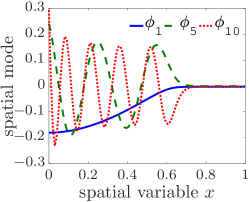
Refer to caption
(a) Spatial modes
Refer to caption
(b) Fixed temporal modes, T-HOSVD
Refer to caption
(c) Fixed temporal modes, ST-HOSVD
Refer to caption
(d) Tailored temporal modes for spatial mode ϕ1subscriptbold-italic-ϕ1\boldsymbol{\phi}_{1}
Refer to caption
(e) Tailored temporal modes for spatial mode ϕ5subscriptbold-italic-ϕ5\boldsymbol{\phi}_{5}
Refer to caption
(f) Tailored temporal modes for spatial mode ϕ10subscriptbold-italic-ϕ10\boldsymbol{\phi}_{10}
Fig. 2: Burgers’ equation. Spatial and temporal modes computed using different tensor-decomposition techniques (see Section 5.1).

7.1.2 Model predictions

We now compare the methods for fixed values of their parameters, and for two randomly selected online points 𝝁1=(1.35,0.0229)𝒟trainsuperscript𝝁11.350.0229subscript𝒟train\boldsymbol{\mu}^{1}=(1.35,0.0229)\not\in\mathcal{D}_{\text{train}} and 𝝁2=(1.45,0.0201)𝒟trainsuperscript𝝁21.450.0201subscript𝒟train\boldsymbol{\mu}^{2}=(1.45,0.0201)\not\in\mathcal{D}_{\text{train}}. Table 1 reports the method parameter values and the associated performance of the methods. Figure 3 reports snapshots of the methods’ responses for t{0,0.1665,0.3332,0.5}𝑡00.16650.33320.5t\in\{0,0.1665,0.3332,0.5\}.

method LSPG GNAT ST-LSPG-1 ST-LSPG-2 ST-GNAT-1 ST-GNAT-2
nssubscript𝑛𝑠{n_{s}} 15 15 15 15 15 15
nzsubscript𝑛𝑧n_{z} 55
nrsubscript𝑛𝑟n_{r} 55
ntisuperscriptsubscript𝑛𝑡𝑖n_{t}^{i} 2 2
ntsubscript𝑛𝑡n_{t} 20 20
n¯ssubscript¯𝑛𝑠\bar{n}_{s} 30 30
n¯tsubscript¯𝑛𝑡\bar{n}_{t} 120 120
nr,ssubscript𝑛𝑟𝑠{n_{r,s}} 100 100
nr,tisuperscriptsubscript𝑛𝑟𝑡𝑖n_{r,t}^{i} 3 10
spatiotemporal dimension 3×1043superscript1043\times 10^{4} 3×1043superscript1043\times 10^{4} 30 300 30 300
relative error for 𝝁1superscript𝝁1\boldsymbol{\mu}^{1} 0.00074 0.011 0.0025 0.0011 0.0058 0.0063
speedup for 𝝁1superscript𝝁1\boldsymbol{\mu}^{1} 0.82 0.34 0.34 0.079 7.19 1.78
relative error for 𝝁2superscript𝝁2\boldsymbol{\mu}^{2} 0.0012 0.017 0.0038 0.0040 0.0077 0.0082
speedup for 𝝁2superscript𝝁2\boldsymbol{\mu}^{2} 0.80 0.39 0.33 0.080 6.22 1.72
Table 1: Burgers’ equation. ROM method performance for fixed method parameters at randomly selected online points 𝝁1=(1.35,0.0229)𝒟trainsuperscript𝝁11.350.0229subscript𝒟train\boldsymbol{\mu}^{1}=(1.35,0.0229)\not\in\mathcal{D}_{\text{train}} and 𝝁2=(1.45,0.0201)𝒟trainsuperscript𝝁21.450.0201subscript𝒟train\boldsymbol{\mu}^{2}=(1.45,0.0201)\not\in\mathcal{D}_{\text{train}}.
Refer to caption
(a) 𝝁=(1.35,0.0229)𝒟train𝝁1.350.0229subscript𝒟train\boldsymbol{\mu}=(1.35,0.0229)\not\in\mathcal{D}_{\text{train}}
Refer to caption
(b) 𝝁=(1.45,0.0201)𝒟train𝝁1.450.0201subscript𝒟train\boldsymbol{\mu}=(1.45,0.0201)\not\in\mathcal{D}_{\text{train}}
Fig. 3: Burgers’ equation. Method solutions for t{0,0.1665,0.3332,0.5}𝑡00.16650.33320.5t\in\{0,0.1665,0.3332,0.5\} corresponding to method parameters reported in Table 1.

First, note that all ROMs generate accurate responses for this particular combination of parameters, as the relative errors are less than 1% in all cases. Second, note that LSPG generates the most accurate responses, but fails to generate any speedup due to its lack of hyper-reduction. GNAT also fails to generate speedup in this case due to the relatively small spatial dimension of the FOM and the larger number of Newton iterations required for convergence relative to LSPG. The proposed ST-LSPG methods incur slightly larger errors than the LSPG method, but they do so with orders of magnitude fewer space–time degrees of freedom. This highlights the promise of performing projection in both space and time: the dimensionality of the problem can be significantly reduced while retaining high levels of accuracy. However, due to their lack of hyper-reduction, the ST-LSPG methods do not generate speedups. Finally, by employing hyper-reduction, the ST-GNAT methods generate very accurate predictions with significant speedups. We note that ST-LSPG-1 and ST-GNAT-1 exhibit better overall performance than ST-LSPG-2 and ST-GNAT-2, respectively; this suggests that employing tailored temporal subspaces enables similar accuracy to be achieved using far fewer degrees of freedom, as each temporal basis vector is tailored to its associated spatial basis vector.

7.1.3 Method-parameter study

This section compares the performance of the ROM methods across a variation of all method parameters. This study is essential to objectively compare the methods, as the particular method-parameter values employed in Section 7.1.2 did not necessarily yield optimal performance for a given method. For this reason, we subject each model to a parameter study wherein each model parameter is varied between specified limits; Table 2 reports the tested parameter values for each method. We consider all elements in the resulting set if they satisfy the following constraints: 1.5nsn¯rnz1.5subscript𝑛𝑠subscript¯𝑛𝑟subscript𝑛𝑧1.5{n_{s}}\leq\bar{n}_{r}\leq n_{z} for GNAT and 1.5nstn¯rn¯sn¯t1.5subscript𝑛𝑠𝑡subscript¯𝑛𝑟subscript¯𝑛𝑠subscript¯𝑛𝑡1.5{n_{st}}\leq\bar{n}_{r}\leq\bar{n}_{s}\bar{n}_{t} for ST-GNAT-1 and ST-GNAT-2. From these results, we then construct a Pareto front for each method, which is characterized by the method parameters that minimize the competing objectives of relative error and relative wall time.

method LSPG GNAT ST-LSPG-1 ST-LSPG-2 ST-GNAT-1 ST-GNAT-2
nssubscript𝑛𝑠{n_{s}} {10×i}i=15superscriptsubscript10𝑖𝑖15\{10\times i\}_{i=1}^{5} {10×i}i=15superscriptsubscript10𝑖𝑖15\{10\times i\}_{i=1}^{5} {10×i}i=15superscriptsubscript10𝑖𝑖15\{10\times i\}_{i=1}^{5} {10×i}i=15superscriptsubscript10𝑖𝑖15\{10\times i\}_{i=1}^{5} {10×i}i=15superscriptsubscript10𝑖𝑖15\{10\times i\}_{i=1}^{5} {10×i}i=15superscriptsubscript10𝑖𝑖15\{10\times i\}_{i=1}^{5}
nzsubscript𝑛𝑧n_{z} {20,30,40,60,80,90}203040608090\{20,30,40,60,80,90\}
nrsubscript𝑛𝑟n_{r} {20,30,40,60,80,90}203040608090\{20,30,40,60,80,90\}
ntisuperscriptsubscript𝑛𝑡𝑖n_{t}^{i} {3,4,5,6,8}34568\{3,4,5,6,8\} {3,4,5,6,8}34568\{3,4,5,6,8\}
ntsubscript𝑛𝑡n_{t} {5,10,20,30}5102030\{5,10,20,30\} {5,10,20,30}5102030\{5,10,20,30\}
n¯ssubscript¯𝑛𝑠\bar{n}_{s} {30,40}3040\{30,40\} {30,40,60,70,80}3040607080\{30,40,60,70,80\}
n¯tsubscript¯𝑛𝑡\bar{n}_{t} {60,120}60120\{60,120\} {120}120\{120\}
nr,ssubscript𝑛𝑟𝑠{n_{r,s}} {100}100\{100\} {100}100\{100\}
nr,tisuperscriptsubscript𝑛𝑟𝑡𝑖n_{r,t}^{i} {3}3\{3\} {10}10\{10\}
Table 2: Burgers’ equation. Parameters used for the method-parameter study. The set of tested parameters comprises the Cartesian product of the specified parameter sets. We consider all elements in the resulting set if they satisfy the following guidelines: 1.5nsn¯rnz1.5subscript𝑛𝑠subscript¯𝑛𝑟subscript𝑛𝑧1.5{n_{s}}\leq\bar{n}_{r}\leq n_{z} for GNAT and 1.5nstn¯rn¯sn¯t1.5subscript𝑛𝑠𝑡subscript¯𝑛𝑟subscript¯𝑛𝑠subscript¯𝑛𝑡1.5{n_{st}}\leq\bar{n}_{r}\leq\bar{n}_{s}\bar{n}_{t} for ST-GNAT-1 and ST-GNAT-2.

Figure 4 reports these Pareto fronts for the two online points, as well as an ‘overall’ Pareto front that selects the Pareto-optimal methods across all parameter variations. Table 3 reports values of the method parameters that yielded Pareto-optimal performance. The proposed ST-GNAT-1 method is Pareto-optimal for relative wall times less than one (i.e., faster than the FOM simulation). While the proposed ST-GNAT-2 method does produce speedups, it is dominated by ST-GNAT-1; this provides further evidence of the advantage of employing a tailored relative to a fixed temporal basis. We note that the worst-performing methods correspond to the ST-LSPG-1, and ST-LSPG-2 methods, as their lack of hyper-reduction leads to significant wall times that far exceed that of the FOM. Further, we note for a fixed error below a certain threshold, the ST-GNAT-1 method is nearly two orders of magnitude faster than the original GNAT method; this can be attributed to the fact that this approach reduces both the spatial and temporal complexities of the FOM. Finally, we note that because the spatial trial subspace employed by LSPG and GNAT has a (relatively large) spatiotemporal dimension of nsNtsubscript𝑛𝑠subscript𝑁𝑡{n_{s}}{N_{t}}, while the space–time trial subspace employed by ST-LSPG and ST-LSPG has a (relatively small) spatiotemporal dimension of nst(nsNt)annotatedsubscript𝑛𝑠𝑡much-less-thanabsentsubscript𝑛𝑠subscript𝑁𝑡{n_{st}}(\ll{n_{s}}{N_{t}}), the LSPG and GNAT methods are able to generate smaller errors than the space–time methods. However, this is achieved at significant computational cost that exceeds that of the FOM in this case (i.e., relative wall times greater than one). Thus, for this problem, LSPG is Pareto-optimal and outperforms the space–time ROMs for relative errors less than 106superscript10610^{-6}, although this regime is not useful because it incurs relative wall times greater than one.
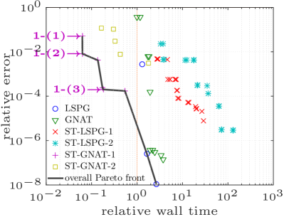
Refer to caption
(a) 𝝁1=(1.35,0.0229)𝒟trainsuperscript𝝁11.350.0229subscript𝒟train\boldsymbol{\mu}^{1}=(1.35,0.0229)\not\in\mathcal{D}_{\text{train}}
Refer to caption
(b) 𝝁2=(1.45,0.0201)𝒟trainsuperscript𝝁21.450.0201subscript𝒟train\boldsymbol{\mu}^{2}=(1.45,0.0201)\not\in\mathcal{D}_{\text{train}}
Fig. 4: Burgers’ equation. Relative error versus relative wall time for varying model parameters reported in Table 1.
label nssubscript𝑛𝑠{n_{s}} ntisuperscriptsubscript𝑛𝑡𝑖n_{t}^{i} n¯ssubscript¯𝑛𝑠\bar{n}_{s} n¯tsubscript¯𝑛𝑡\bar{n}_{t} nr,ssubscript𝑛𝑟𝑠{n_{r,s}} nr,tisuperscriptsubscript𝑛𝑟𝑡𝑖n_{r,t}^{i}
1-(1) 10 3 30 60 100 3
1-(2) 10 4 30 60 100 3
1-(3) 30 3 40 120 100 3
2-(1) 20 3 30 60 100 10
2-(2) 30 3 40 120 100 10
Table 3: Burgers’ equation. Parameter values yielding Pareto-optimal performance for the ST-GNAT-1 method. Figure 4 provides labels.

7.2 Quasi 1D Euler equation

We now consider a parameterized quasi-1D Euler equation associated with modeling inviscid compressible flow in a one-dimensional converging–diverging nozzle with a continuously varying cross-sectional area [33, Chapter 13]; Figure 5 depicts the problem geometry. The governing system of nonlinear PDEs is

(7.3) 𝒘t+1A(𝒇(𝒘)A)x=𝒒(𝒘),x[0,1]m,t[0,T],formulae-sequence𝒘𝑡1𝐴𝒇𝒘𝐴𝑥𝒒𝒘formulae-sequencefor-all𝑥01mfor-all𝑡0𝑇\frac{\partial\boldsymbol{w}}{\partial t}+\frac{1}{A}\frac{\partial(\boldsymbol{f}(\boldsymbol{w})A)}{\partial x}=\boldsymbol{q}(\boldsymbol{w}),\quad\forall x\in[0,1]\ \text{m},\quad\forall t\in[0,T],

where T=0.6𝑇0.6T=0.6 s and

(7.4) 𝒘=[ρρue],𝒇(𝒘)=[ρuρu2+p(e+p)u],𝒒(𝒘)=[0pAAx0],p=(γ1)ρϵ,ϵ=eρu22,A=A(x).formulae-sequence𝒘matrix𝜌𝜌𝑢𝑒formulae-sequence𝒇𝒘matrix𝜌𝑢𝜌superscript𝑢2𝑝𝑒𝑝𝑢formulae-sequence𝒒𝒘matrix0𝑝𝐴𝐴𝑥0formulae-sequence𝑝𝛾1𝜌italic-ϵformulae-sequenceitalic-ϵ𝑒𝜌superscript𝑢22𝐴𝐴𝑥\boldsymbol{w}=\begin{bmatrix}\rho\\ \rho u\\ e\end{bmatrix},\quad\boldsymbol{f}(\boldsymbol{w})=\begin{bmatrix}\rho u\\ \rho u^{2}+p\\ (e+p)u\end{bmatrix},\quad\boldsymbol{q}(\boldsymbol{w})=\begin{bmatrix}0\\ \frac{p}{A}\frac{\partial A}{\partial x}\\ 0\end{bmatrix},\quad p=(\gamma-1)\rho\epsilon,\quad\epsilon=\frac{e}{\rho}-\frac{u^{2}}{2},\quad A=A(x).

Here, ρ𝜌\rho denotes density, u𝑢u denotes velocity, p𝑝p denotes pressure, ϵitalic-ϵ\epsilon denotes potential energy per unit mass, e𝑒e denotes total energy density, γ𝛾\gamma denotes the specific heat ratio, and A𝐴A denotes the converging–diverging nozzle cross-sectional area. We employ a specific heat ratio of γ=1.3𝛾1.3\gamma=1.3, a specific gas constant of R=355.4𝑅355.4R=355.4 m2/s2/Ksuperscriptm2superscripts2K\text{m}^{2}/\text{s}^{2}/\text{K}, a total temperature of Tt=300subscript𝑇𝑡300T_{t}=300 K, and a total pressure of pt=106subscript𝑝𝑡superscript106p_{t}=10^{6} N/m2Nsuperscriptm2\text{N}/\text{m}^{2}. The cross-sectional area A(x)𝐴𝑥A(x) is determined by a cubic spline interpolation over the points (x,A(x)){(0,0.2),(0.25,0.173),(0.5,0.17),(0.75,0.173),(1,0.2)}𝑥𝐴𝑥00.20.250.1730.50.170.750.17310.2(x,A(x))\in\{(0,0.2),(0.25,0.173),(0.5,0.17),(0.75,0.173),(1,0.2)\}, which results in

(7.5) A(x)={0.288x3+0.4080x20.1920x+0.2,x[0,0.25)m0.288(x0.25)3+0.1920(x0.25)20.0420(x0.25)+0.1730,x[0.25,0.5)m0.288(x0.5)30.0240(x0.5)2+0.17,x[0.5,0.75)m0.288(x0.75)3+0.1920(x0.75)2+0.0420(x0.75)+0.1730,x[0.75,1]m.𝐴𝑥cases0.288superscript𝑥30.4080superscript𝑥20.1920𝑥0.2𝑥00.25m0.288superscript𝑥0.2530.1920superscript𝑥0.2520.0420𝑥0.250.1730𝑥0.250.5m0.288superscript𝑥0.530.0240superscript𝑥0.520.17𝑥0.50.75m0.288superscript𝑥0.7530.1920superscript𝑥0.7520.0420𝑥0.750.1730𝑥0.751mA(x)=\left\{\begin{array}[]{ll}-0.288x^{3}+0.4080x^{2}-0.1920x+0.2,&x\in[0,0.25)\ \text{m}\\ -0.288(x-0.25)^{3}+0.1920(x-0.25)^{2}-0.0420(x-0.25)+0.1730,&x\in[0.25,0.5)\ \text{m}\\ 0.288(x-0.5)^{3}-0.0240(x-0.5)^{2}+0.17,&x\in[0.5,0.75)\ \text{m}\\ 0.288(x-0.75)^{3}+0.1920(x-0.75)^{2}+0.0420(x-0.75)+0.1730,&x\in[0.75,1]\ \text{m}.\end{array}\right.

We assume a perfect gas that obeys the ideal gas law (i.e., p=ρRT𝑝𝜌𝑅𝑇p=\rho RT). The initial flow field is created in several steps. First, the following isentropic relations are used to generate a zero pressure-gradient flow field:

(7.6) M(x)=MmAmA(x)(1+γ12M(x)21+γ12Mm2)γ+12(γ1),p(x)=pt(1+γ12M(x)2)γγ1T(x)=Tt(1+γ12M(x)2)1,ρ(x)=p(x)RT(x),c(x)=γp(x)ρ(x),u(x)=M(x)c(x),\displaystyle\begin{split}M(x)&=\frac{M_{m}A_{m}}{A(x)}\left(\frac{1+\frac{\gamma-1}{2}M(x)^{2}}{1+\frac{\gamma-1}{2}M_{m}^{2}}\right)^{\frac{\gamma+1}{2(\gamma-1)}},\quad p(x)=p_{t}\left(1+\frac{\gamma-1}{2}M(x)^{2}\right)^{\frac{-\gamma}{\gamma-1}}\\ T(x)&=T_{t}\left(1+\frac{\gamma-1}{2}M(x)^{2}\right)^{-1},\quad\rho(x)=\frac{p(x)}{RT(x)},\quad c(x)=\sqrt{\gamma\frac{p(x)}{\rho(x)}},\quad u(x)=M(x)c(x),\end{split}

where a subscript m𝑚m indicates the flow quantity at x=0.5𝑥0.5x=0.5 m, and M𝑀M denotes the Mach number. Then, a shock is placed at x=0.85𝑥0.85x=0.85 m of the flow field. We use the jump relations for a stationary shock and the perfect gas equation of state to derive the velocity across the shock u2subscript𝑢2u_{2}, which satisfies the quadratic equation

(7.7) (12γγ1)u22+γγ1nmu2h=0.12𝛾𝛾1superscriptsubscript𝑢22𝛾𝛾1𝑛𝑚subscript𝑢20\left(\frac{1}{2}-\frac{\gamma}{\gamma-1}\right)u_{2}^{2}+\frac{\gamma}{\gamma-1}\frac{n}{m}u_{2}-h=0.

Here, m:=ρ2u2=ρ1u1assign𝑚subscript𝜌2subscript𝑢2subscript𝜌1subscript𝑢1m:=\rho_{2}u_{2}=\rho_{1}u_{1}, n:=ρ2u22+p2=ρ1u12+p1assign𝑛subscript𝜌2superscriptsubscript𝑢22subscript𝑝2subscript𝜌1superscriptsubscript𝑢12subscript𝑝1n:=\rho_{2}u_{2}^{2}+p_{2}=\rho_{1}u_{1}^{2}+p_{1}, h:=(e2+p2)/ρ2=(e1+p1)/ρ1assignsubscript𝑒2subscript𝑝2subscript𝜌2subscript𝑒1subscript𝑝1subscript𝜌1h:=(e_{2}+p_{2})/\rho_{2}=(e_{1}+p_{1})/\rho_{1}, and subscripts 111 and 222 denote a flow quantity to the left and to the right of the shock, respectively. We employ the solution u2subscript𝑢2u_{2} to Eq. (7.7), which leads to a discontinuity (i.e., shock). Finally, the exit pressure is increased to a factor Pexitsubscript𝑃exitP_{\text{exit}} of its original value in order to generate transient dynamics.

Refer to caption
Fig. 5: Quasi-1D Euler. Schematic figures of converging-diverging nozzle.

Applying a finite-volume spatial discretization with 50 equally spaced control volumes and fully implicit boundary conditions leads to a parameterized system of nonlinear ODEs consistent with Eq. (2.1) with Ns=150subscript𝑁𝑠150N_{s}=150 spatial degrees of freedom. The Roe flux difference vector splitting method is used to compute the flux at each intercell face [33, Chapter 9]. For time discretization, we again apply the backward Euler scheme and a uniform time step of Δt=0.001Δ𝑡0.001\Delta t=0.001 s, leading to Nt=600subscript𝑁𝑡600{N_{t}}=600.

For this problem, we use the following two parameters: the pressure factor μ1=Pexitsubscript𝜇1subscript𝑃exit\mu_{1}=P_{\text{exit}} and the Mach number at the middle of the nozzle μ2=Mmsubscript𝜇2subscript𝑀𝑚\mu_{2}=M_{m}. All ROMs employ a training set at which the FOM is solved of 𝒟train={1.7+0.01i}i=03×{1.7,1.72}subscript𝒟trainsuperscriptsubscript1.70.01𝑖𝑖031.71.72\mathcal{D}_{\text{train}}=\{1.7+0.01i\}_{i=0}^{3}\times\{1.7,1.72\} such that ntrain=8subscript𝑛train8n_{\text{train}}=8.

7.2.1 Space–time bases

Figure 6 plots several spatial and temporal modes computed using the three different techniques proposed in Section 5.1. As with the Burgers equation, the ‘fixed’ temporal modes are nearly identical, regardless of whether the T-HOSVD or ST-HOSVD is employed, rendering the ST-HOSVD more appealing due to its reduced computational cost. In addition, the tailored temporal modes are significantly different, with the temporal basis exhibiting higher frequencies for higher-index spatial modes as expected.
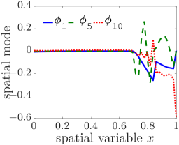
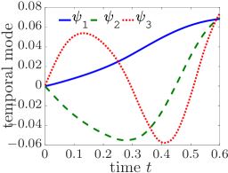
Refer to caption
(a) Spatial modes
Refer to caption
(b) Fixed temporal modes, T-HOSVD
Refer to caption
(c) Fixed temporal modes, ST-HOSVD
Refer to caption
(d) Tailored temporal modes for spatial mode ϕ1subscriptbold-italic-ϕ1\boldsymbol{\phi}_{1}
Refer to caption
(e) Tailored temporal modes for spatial mode ϕ5subscriptbold-italic-ϕ5\boldsymbol{\phi}_{5}
Refer to caption
(f) Tailored temporal modes for spatial mode ϕ10subscriptbold-italic-ϕ10\boldsymbol{\phi}_{10}
Fig. 6: Quasi-1D Euler equation. Spatial and temporal modes computed using different techniques (see Section 5.1).

7.2.2 Model predictions

We now compare the methods for fixed values of their parameters, and for two randomly selected online points 𝝁1=(1.7125,1.71)𝒟trainsuperscript𝝁11.71251.71subscript𝒟train\boldsymbol{\mu}^{1}=(1.7125,1.71)\not\in\mathcal{D}_{\text{train}} and 𝝁2=(1.7225,1.705)𝒟trainsuperscript𝝁21.72251.705subscript𝒟train\boldsymbol{\mu}^{2}=(1.7225,1.705)\not\in\mathcal{D}_{\text{train}}. Table 4 reports the method parameter values and the associated performance of the methods. Figure 7 reports snapshots of the methods’ responses for t{0,T}𝑡0𝑇t\in\{0,T\}.

method LSPG GNAT ST-LSPG-1 ST-LSPG-2 ST-GNAT-1 ST-GNAT-2
nssubscript𝑛𝑠{n_{s}} 50 50 50 50 50 50
nzsubscript𝑛𝑧n_{z} 145
nrsubscript𝑛𝑟n_{r} 145
ntisuperscriptsubscript𝑛𝑡𝑖n_{t}^{i} 3 3
ntsubscript𝑛𝑡n_{t} 30 30
n¯ssubscript¯𝑛𝑠\bar{n}_{s} 120 140
n¯tsubscript¯𝑛𝑡\bar{n}_{t} 20 100
nr,ssubscript𝑛𝑟𝑠{n_{r,s}} 150 150
nr,tisuperscriptsubscript𝑛𝑟𝑡𝑖n_{r,t}^{i} 10 10
spatiotemporal dimension 3×1043superscript1043\times 10^{4} 3×1043superscript1043\times 10^{4} 150 1.5×1031.5superscript1031.5\times 10^{3} 150 1.5×1031.5superscript1031.5\times 10^{3}
relative error for 𝝁1superscript𝝁1\boldsymbol{\mu}^{1} 7.78×1067.78superscript1067.78\times 10^{-6} 0.55 0.012 6.3×1046.3superscript1046.3\times 10^{-4} 0.0023 0.0048
speedup for 𝝁1superscript𝝁1\boldsymbol{\mu}^{1} 0.77 1.04 0.84 0.58 21.79 0.49
relative error for 𝝁2superscript𝝁2\boldsymbol{\mu}^{2} 8.31×1068.31superscript1068.31\times 10^{-6} 0.026 0.0076 0.0021 0.0025 0.0040
speedup for 𝝁2superscript𝝁2\boldsymbol{\mu}^{2} 0.81 1.01 0.85 0.41 22.52 2.79
Table 4: Quasi-1D Euler equation. ROM method performance for fixed method parameters at randomly selected online points 𝝁1=(1.7125,1.71)𝒟trainsuperscript𝝁11.71251.71subscript𝒟train\boldsymbol{\mu}^{1}=(1.7125,1.71)\not\in\mathcal{D}_{\text{train}} and 𝝁2=(1.7225,1.705)𝒟trainsuperscript𝝁21.72251.705subscript𝒟train\boldsymbol{\mu}^{2}=(1.7225,1.705)\not\in\mathcal{D}_{\text{train}}.
Refer to caption
(a) 𝝁=(1.7125,1.71)𝒟train𝝁1.71251.71subscript𝒟train\boldsymbol{\mu}=(1.7125,1.71)\not\in\mathcal{D}_{\text{train}}
Refer to caption
(b) 𝝁=(1.7225,1.705)𝒟train𝝁1.72251.705subscript𝒟train\boldsymbol{\mu}=(1.7225,1.705)\not\in\mathcal{D}_{\text{train}}
Fig. 7: Quasi-1D Euler equation. Method solutions for t{0,T}𝑡0𝑇t\in\{0,T\} corresponding to method parameters reported in Table 4.

Conclusions are similar to those derived from the Burgers’ equation results. First, note that all ROMs except for GNAT in the case of 𝝁1superscript𝝁1\boldsymbol{\mu}^{1} generate accurate responses, as the relative errors are less than 3% in all cases. Second, as before, LSPG generates the most accurate responses, but fails to generate any speedup due to its lack of hyper-reduction. The proposed ST-LSPG methods incur sub-2% errors, but they do so with orders of magnitude fewer spatiotemporal degrees of freedom relative to the LSPG and GNAT methods, which highlights the promise of performing projection in both space and time. Again, as these methods do not employ hyper-reduction, they do not generate speedups. Finally, the ST-GNAT methods generate both accurate predictions with significant speedups. We note that ST-GNAT-1 performs better than ST-GNAT-2, providing further evidence of the ability of tailored bases to produce accurate responses with fewer degrees of freedom.

7.2.3 Method-parameter study

We again compare the performance of the ROM methods across a wide variation of all method parameters. Table 5 reports the tested parameter values for each method. We consider all elements in the resulting set if they satisfy constraints 1.5nsn¯rnz1.5subscript𝑛𝑠subscript¯𝑛𝑟subscript𝑛𝑧1.5{n_{s}}\leq\bar{n}_{r}\leq n_{z} for GNAT and 1.5nstn¯rn¯sn¯t1.5subscript𝑛𝑠𝑡subscript¯𝑛𝑟subscript¯𝑛𝑠subscript¯𝑛𝑡1.5{n_{st}}\leq\bar{n}_{r}\leq\bar{n}_{s}\bar{n}_{t} for ST-GNAT-1 and ST-GNAT-2. From these results, we then construct a Pareto front for each method, which is characterized by the method parameters that minimize the competing objectives of relative error and relative wall time.

method LSPG GNAT ST-LSPG-1 ST-LSPG-2 ST-GNAT-1 ST-GNAT-2
nssubscript𝑛𝑠{n_{s}} {10×i}i=16superscriptsubscript10𝑖𝑖16\{10\times i\}_{i=1}^{6} {10×i}i=16superscriptsubscript10𝑖𝑖16\{10\times i\}_{i=1}^{6} {10×i}i=16superscriptsubscript10𝑖𝑖16\{10\times i\}_{i=1}^{6} {10×i}i=16superscriptsubscript10𝑖𝑖16\{10\times i\}_{i=1}^{6} {10×i}i=16superscriptsubscript10𝑖𝑖16\{10\times i\}_{i=1}^{6} {10×i}i=16superscriptsubscript10𝑖𝑖16\{10\times i\}_{i=1}^{6}
nzsubscript𝑛𝑧n_{z} {10×i}i=210{120,145}superscriptsubscript10𝑖𝑖210120145\{10\times i\}_{i=2}^{10}\cup\{120,145\}
nrsubscript𝑛𝑟n_{r} {10×i}i=210{120,145}superscriptsubscript10𝑖𝑖210120145\{10\times i\}_{i=2}^{10}\cup\{120,145\}
ntisuperscriptsubscript𝑛𝑡𝑖n_{t}^{i} {i}i=38superscriptsubscript𝑖𝑖38\{i\}_{i=3}^{8} {i}i=38superscriptsubscript𝑖𝑖38\{i\}_{i=3}^{8}
ntsubscript𝑛𝑡n_{t} {10×i}i=25superscriptsubscript10𝑖𝑖25\{10\times i\}_{i=2}^{5} {10×i}i=25superscriptsubscript10𝑖𝑖25\{10\times i\}_{i=2}^{5}
n¯ssubscript¯𝑛𝑠\bar{n}_{s} {120}120\{120\} {140}140\{140\}
n¯tsubscript¯𝑛𝑡\bar{n}_{t} {10,20,30,40,60}1020304060\{10,20,30,40,60\} {30,50,100,150}3050100150\{30,50,100,150\}
nr,ssubscript𝑛𝑟𝑠{n_{r,s}} 150 150
nr,tisuperscriptsubscript𝑛𝑟𝑡𝑖n_{r,t}^{i} 10 10
Table 5: Quasi-1D Euler equation. Parameters used for the method-parameter study. The set of tested parameters comprises the Cartesian product of the specified parameter sets. We consider all elements in the resulting set if they satisfy the following guidelines: 1.5nsn¯rnz1.5subscript𝑛𝑠subscript¯𝑛𝑟subscript𝑛𝑧1.5{n_{s}}\leq\bar{n}_{r}\leq n_{z} for GNAT and 1.5nstn¯rn¯sn¯t1.5subscript𝑛𝑠𝑡subscript¯𝑛𝑟subscript¯𝑛𝑠subscript¯𝑛𝑡1.5{n_{st}}\leq\bar{n}_{r}\leq\bar{n}_{s}\bar{n}_{t} for ST-GNAT-1 and ST-GNAT-2.

Figure 8 reports these Pareto fronts for the two online points, as well as an overall Pareto front that selects the Pareto-optimal methods across all parameter variations. Table 6 reports values of the method parameters that yielded Pareto-optimal performance. These results show that—as before—the proposed ST-GNAT-1 method is Pareto optimal for relative wall time less than 0.9 and relative errors less than 20%. While the proposed ST-GNAT-2 method produces speedups, it is again dominated by ST-GNAT-1, further highlighting the advantage of tailored versus fixed temporal bases. Again, the worst-performing methods correspond to the ST-LSPG-1, and ST-LSPG-2 methods, as their lack of hyper-reduction leads to significant wall times that far exceed that of the FOM. Further, we note that for a fixed error below a certain threshold, the ST-GNAT-1 method is over one order of magnitude faster than the original GNAT method; this can be attributed to the fact that this approach reduces both the spatial and temporal complexities of the FOM. Finally, we again note that LSPG is Pareto-optimal and outperforms the space–time ROMs for extremely small relative errors less than approximately 3×1053superscript1053\times 10^{-5} due to the higher spatiotemporal dimensionality of the spatial trial subspace; however, this regime is not useful for this problem, as it leads to LSPG models roughly as expensive as the FOM (i.e., relative wall times near one).
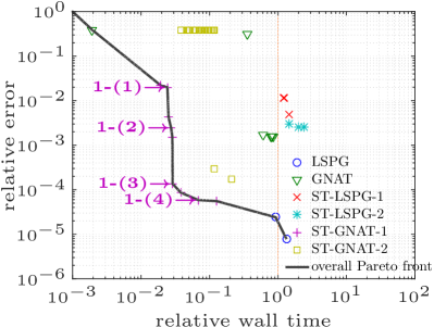
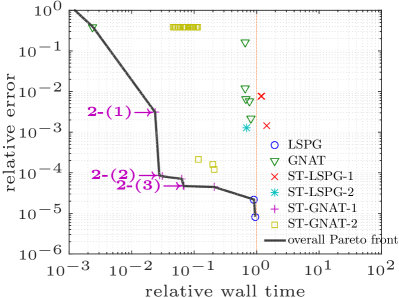
Refer to caption
(a) 𝝁=(1.7125,1.71)𝒟train𝝁1.71251.71subscript𝒟train\boldsymbol{\mu}=(1.7125,1.71)\not\in\mathcal{D}_{\text{train}}
Refer to caption
(b) 𝝁=(1.7225,1.705)𝒟train𝝁1.72251.705subscript𝒟train\boldsymbol{\mu}=(1.7225,1.705)\not\in\mathcal{D}_{\text{train}}
Fig. 8: Quasi-1D Euler equation. Relative error versus relative wall time for varying model parameters reported in Table 5.
label nssubscript𝑛𝑠{n_{s}} ntisuperscriptsubscript𝑛𝑡𝑖n_{t}^{i} n¯ssubscript¯𝑛𝑠\bar{n}_{s} n¯tsubscript¯𝑛𝑡\bar{n}_{t} nr,ssubscript𝑛𝑟𝑠{n_{r,s}} nr,tisuperscriptsubscript𝑛𝑟𝑡𝑖n_{r,t}^{i}
1-(1) 10 3 120 10 150 10
1-(2) 60 3 120 10 150 10
1-(3) 30 4 120 10 150 10
1-(4) 50 8 120 10 150 10
2-(1) 30 3 120 10 150 10
2-(2) 50 4 120 10 150 10
2-(3) 60 7 120 10 150 10
Table 6: Quasi-1D Euler equation. Parameter values yielding Pareto-optimal performance for the ST-GNAT-1 method. Figure 8 provides labels.

8 Conclusions

This work proposed a model-reduction method for nonlinear dynamical systems based on space–time least-squares Petrov–Galerkin projection. The method computes optimal approximations by minimizing the discrete space–time residual over all elements in a low-dimensional space–time trial subspace in a weighted 2superscript2\ell^{2}-norm. Advantages of the method include:

  • its ability to reduce both the spatial and temporal dimensions of the dynamical system (Remark 4.1),

  • a priori error bounds that bound the solution error by the best space–time approximation error and whose stability constants exhibit subquadratic growth in time (Section 6),

  • applicability to general nonlinear dynamical systems,

  • hyper-reduction that reduces the complexity in the presence of general nonlinearities (Section 4.3), and

  • its ability to extract multiple space–time basis vectors from each training simulation via tensor decomposition (Section 6).

In addition to introducing the novel ST-LSPG method, this work proposed specific approaches to computing the method’s ingredients: the space–time trial subspace (Section 5.1), the space–time residual basis in the case of ST–GNAT (Section 5.2), the sampling matrix in the case of hyper-reduction (Section 5.3), and the initial guess used in the Gauss–Newton method applied to solve the nonlinear least-squares problem (Section 5.4). Numerical experiments demonstrated the ability of the proposed method to generate orders-of-magnitude speedups over existing spatial-projection-based ROMs without sacrificing accuracy.

Future work entails implementing the method in parallel computational-mechanics codes, devising techniques to reduce the amount of storage required for the state and residual tensors, and assessing the effect of different time integrators—as well as adaptive time-stepping—on method performance.

Acknowledgments

The authors gratefully acknowledge Tamara Kolda and Grey Ballard for insightful discussions that led to the tensor-decomposition approaches for computing the space–time trial subspace. The authors also acknowledge Professors Benjamin Peherstorfer and Masayuki Yano for useful comments received at the Model Reduction for Parametrized Systems (MoRePaS) III workshop and the 2017 SIAM Conference on Computational Science and Engineering, respectively. The authors also gratefully acknowledge the helpful comments provided by the anonymous reviewers. This work was performed at Sandia National Laboratories and was supported by the LDRD program (project 190968). Sandia National Laboratories is a multimission laboratory managed and operated by National Technology and Engineering Solutions of Sandia, LLC., a wholly owned subsidiary of Honeywell International, Inc., for the U.S. Department of Energy’s National Nuclear Security Administration under contract DE-NA-0003525. Lawrence Livermore National Laboratory is operated by Lawrence Livermore National Security, LLC, for the U.S. Department of Energy, National Nuclear Security Administration under Contract DE-AC52-07NA27344.

References

  • [1] P. Astrid, S. Weiland, K. Willcox, and T. Backx, Missing point estimation in models described by proper orthogonal decomposition, IEEE Transactions on Automatic Control, 53 (2008), pp. 2237–2251.
  • [2] W. Austin, G. Ballard, and T. G. Kolda, Parallel tensor compression for large-scale scientific data, arXiv preprint arXiv:1510.06689, (2015).
  • [3] I. Babuska, R. Tempone, and G. E. Zouraris, Galerkin finite element approximations of stochastic elliptic partial differential equations, SIAM Journal on Numerical Analysis, 42 (2004), pp. 800–825.
  • [4] A. T. Barker, T. Rees, and M. Stoll, A fast solver for an 1subscript1\mathcal{H}_{1} regularized PDE-constrained optimization problem, Communications in Computational Physics, 19 (2016), pp. 143–167.
  • [5] M. Barrault, Y. Maday, N. C. Nguyen, and A. T. Patera, An ‘empirical interpolation’ method: application to efficient reduced-basis discretization of partial differential equations, Comptes Rendus Mathématique Académie des Sciences, 339 (2004), pp. 667–672.
  • [6] M. Baumann, P. Benner, and J. Heiland, Space-time Galerkin POD with application in optimal control of semi-linear parabolic partial differential equations, arXiv preprint arXiv:1611.04050, (2016).
  • [7] R. Bos, X. Bombois, and P. Van den Hof, Accelerating large-scale non-linear models for monitoring and control using spatial and temporal correlations, Proceedings of the American Control Conference, 4 (2004), pp. 3705–3710.
  • [8] K. Carlberg, M. Barone, and H. Antil, Galerkin v. least-squares Petrov–Galerkin projection in nonlinear model reduction, Journal of Computational Physics, 330 (2017), pp. 693–734.
  • [9] K. Carlberg, C. Bou-Mosleh, and C. Farhat, Efficient non-linear model reduction via a least-squares Petrov–Galerkin projection and compressive tensor approximations, International Journal for Numerical Methods in Engineering, 86 (2011), pp. 155–181.
  • [10] K. Carlberg, L. Brencher, B. Haasdonk, and A. Barth, Data-driven time parallelism via forecasting, arXiv preprint arXiv:1610.09049, (2016).
  • [11] K. Carlberg, C. Farhat, J. Cortial, and D. Amsallem, The GNAT method for nonlinear model reduction: effective implementation and application to computational fluid dynamics and turbulent flows, Journal of Computational Physics, 242 (2013), pp. 623–647.
  • [12] K. Carlberg, J. Ray, and B. van Bloemen Waanders, Decreasing the temporal complexity for nonlinear, implicit reduced-order models by forecasting, Computer Methods in Applied Mechanics and Engineering, 289 (2015), pp. 79–103.
  • [13] S. Chaturantabut and D. C. Sorensen, Nonlinear model reduction via discrete empirical interpolation, SIAM Journal on Scientific Computing, 32 (2010), pp. 2737–2764.
  • [14] A. Chirokov, Scattered data interpolation and approximation using radial base functions, MATLAB Centeral Exchange, (Retrieved Feburary 18, 2006).
  • [15] Y. Choi, Simultaneous analysis and design in PDE-constrained optimization, PhD thesis, Stanford University, 2012.
  • [16] Y. Choi, C. Farhat, W. Murray, and M. Saunders, A practical factorization of a Schur complement for PDE-constrained distributed optimal control, Journal of Scientific Computing, 65 (2015), pp. 576–597.
  • [17] P. Constantine and Q. Wang, Residual minimizing model reduction for parameterized nonlinear dynamical systems, SIAM J. Sci. Comput., 34 (2012), pp. A2118–A2144.
  • [18] L. De Lathauwer, B. De Moor, and J. Vandewalle, A multilinear singular value decomposition, SIAM journal on Matrix Analysis and Applications, 21 (2000), pp. 1253–1278.
  • [19] M. Drohmann, B. Haasdonk, and M. Ohlberger, Reduced basis approximation for nonlinear parametrized evolution equations based on empirical operator interpolation, SIAM Journal on Scientific Computing, 34 (2012), pp. A937–A969.
  • [20] R. Elber, Perspective: Computer simulations of long time dynamics, The Journal of Chemical Physics, 144 (2016), p. 060901.
  • [21] R. Everson and L. Sirovich, Karhunen–Loève procedure for gappy data, Journal of the Optical Society of America A, 12 (1995), pp. 1657–1664.
  • [22] R. D. Falgout, S. Freidhoff, T. V. Kolev, S. P. MacLachlan, and J. B. Schroder, Parallel time integration with multigrid, SIAM J. Sci. Comput., 36 (2014), pp. C635–C661.
  • [23] C. Farhat and M. Chandesris, Time-decomposed parallel time-integrators: theory and feasibility studies for fluid, structure, and fluid–structure applications, International Journal for Numerical Methods in Engineering, 58 (2003), pp. 1397–1434.
  • [24] D. Galbally, K. Fidkowski, K. Willcox, and O. Ghattas, Non-linear model reduction for uncertainty quantification in large-scale inverse problems, International Journal for Numerical Methods in Engineering, 81 (2009), pp. 1581–1608.
  • [25] R. G. Ghanem and P. D. Spanos, Stochastic finite elements: a spectral approach, Courier Corporation, 2003.
  • [26] R. Haftka and M. Kamat, Simultaneous nonlinear structural analysis and design, Computational Mechanics, 4 (1989), pp. 409–416.
  • [27] T. Ito and K. Tanikawa, Long-term integrations and stability of planetary orbits in our solar system, Monthly Notices of the Royal Astronomical Society, 336 (2002), pp. 483–500.
  • [28] D. J. Knezevic, N.-C. Nguyen, and A. T. Patera, Reduced basis approximation and a posteriori error estimation for the parametrized unsteady boussinesq equations, Mathematical Models and Methods in Applied Sciences, 21 (2011), pp. 1415–1442.
  • [29] P. Krysl, S. Lall, and J. E. Marsden, Dimensional model reduction in non-linear finite elements dynamics of solids and structures, Int. J. Numer. Meth. Engng, 51 (2001), pp. 479–504.
  • [30] P. A. LeGresley, Application of Proper Orthogonal Decomposition (POD) to Design Decomposition Methods, PhD thesis, Stanford University, 2006.
  • [31] J. Lions, Y. Maday, and G. Turinici, A “parareal” in time discretization of PDEs, Comptes Rendus de l’Academie des Sciences Series I Mathematics, 332 (2001), pp. 661–668.
  • [32] D. J. Lucia, P. S. Beran, and W. A. Silva, Reduced-order modeling: new approaches for computational physics, Progress in Aerospace Sciences, 40 (2004), pp. 51–117.
  • [33] R. MacCormack, Numerical computation of compressible viscous flow, tech. rep., Lecture notes for AA214b and AA214c, Stanford University, 2007.
  • [34] N.-C. Nguyen, G. Rozza, and A. T. Patera, Reduced basis approximation and a posteriori error estimation for the time-dependent viscous Burgers’ equation, Calcolo, 46 (2009), pp. 157–185.
  • [35] J. Nocedal and S. J. Wright, Numerical Optimization, Springer, 2nd ed., 2006.
  • [36] C. E. Orozco and O. N. Ghattas, A reduced SAND method for optimal design of non-linear structures, International Journal for Numerical Methods in Engineering, 40 (1997), pp. 2759–2774.
  • [37] J. W. Pearson and A. J. Wathen, A new approximation of the Schur complement in preconditioners for PDE-constrained optimization, Numerical Linear Algebra with Applications, 19 (2012), pp. 816–829.
  • [38] M. Rathinam and L. R. Petzold, A new look at proper orthogonal decomposition, SIAM Journal on Numerical Analysis, 41 (2003), pp. 1893–1925.
  • [39] T. Rees, M. Stoll, and A. Wathen, All-at-once preconditioning in PDE-constrained optimization, Kybernetika, 46 (2010), pp. 341–360.
  • [40] M. J. Rewienski, A Trajectory Piecewise-Linear Approach to Model Order Reduction of Nonlinear Dynamical Systems, PhD thesis, Massachusetts Institute of Technology, 2003.
  • [41] D. Ryckelynck, A priori hyperreduction method: an adaptive approach, Journal of Computational Physics, 202 (2005), pp. 346–366.
  • [42] B. Space, H. Rabitz, and A. Askar, Long time scale molecular dynamics subspace integration method applied to anharmonic crystals and glasses, The Journal of Chemical Physics, 99 (1993), pp. 9070–9079.
  • [43] Z. A. Taylor, S. Crozier, and S. Ourselin, Real-time surgical simulation using reduced order finite element analysis, in International Conference on Medical Image Computing and Computer-Assisted Intervention, Springer, 2010, pp. 388–395.
  • [44] L. R. Tucker, Some mathematical notes on three-mode factor analysis, Psychometrika, 31 (1966), pp. 279–311.
  • [45] K. Urban and A. Patera, A new error bound for reduced basis approximation of parabolic partial differential equations, Comptes Rendus Mathematique, 350 (2012), pp. 203–207.
  • [46] K. Urban and A. Patera, An improved error bound for reduced basis approximation of linear parabolic problems, Mathematics of Computation, 83 (2014), pp. 1599–1615.
  • [47] N. Vannieuwenhoven, R. Vandebril, and K. Meerbergen, A new truncation strategy for the higher-order singular value decomposition, SIAM Journal on Scientific Computing, 34 (2012), pp. A1027–A1052.
  • [48] S. Volkwein and S. Weiland, An algorithm for Galerkin projections in both time and spatial coordinates, Proc. 17th MTNS, (2006).
  • [49] M. Yano, A space-time Petrov–Galerkin certified reduced basis method: application to the Boussinesq equations, SIAM J. Sci. Comput, 36 (2013), pp. A232–A266.
  • [50] M. Yano, A. T. Patera, and K. Urban, A space-time certified reduced-basis method for Burgers’ equation, Math. Mod. Meth. Appl. S., submitted (2014), pp. 1903–1935.
  • [51] M. J. Zahr, K. Carlberg, D. Amsallem, and C. Farhat, Comparison of model reduction techniques on high-fidelity linear and nonlinear electrical, mechanical, and biological systems, University of California, Berkeley, (2010).