Quasiparticle Breakdown and Spin Hamiltonian of the
Frustrated Quantum Pyrochlore Yb₂Ti₂O₇ in Magnetic Field

Abstract

The frustrated pyrochlore magnet Yb₂Ti₂O₇ has the remarkable property that it orders magnetically, but has no propagating magnons over wide regions of the Brillouin zone. Here we use inelastic neutron scattering to follow how the spectrum evolves in cubic-axis magnetic fields. At high fields we observe in addition to dispersive magnons also a two-magnon continuum, which grows in intensity upon reducing the field and overlaps with the one-magnon states at intermediate fields leading to strong renormalization of the dispersion relations, and magnon decays. Using heat capacity measurements we find that the low and high field regions are smoothly connected with no sharp phase transition, with the spin gap increasing monotonically in field. Through fits to an extensive data set we re-evaluate the spin Hamiltonian finding dominant quantum exchange terms, which we propose are responsible for the anomalously strong fluctuations and quasiparticle breakdown effects observed at low fields.

The lattice of corner-shared tetrahedra realized in cubic A₂B₂O₇ pyrochlores and AB₂O₄ spinels, is a canonical lattice to explore correlated magnetism in the presence of strong geometric frustration effects. In the strongly spin-orbit coupled rare earth pyrochlores, experiment has uncovered materials offering a tremendously rich spectrum of magnetic behavior. Notable examples include classical spin ice physics as in the rare-earth titanates (Ho/Dy)₂Ti₂O₇ where Ising antiferromagnetism leads to an emergent classical electrostatics at low temperatures Castelnovo et al. (2012) and “order-by-disorder” in XY antiferromagnets where thermal and quantum fluctuations lift a large frustration-induced degeneracy resulting in unconventional magnetic order as in Er₂Ti₂O₇ Savary et al. (2012); Zhitomirsky et al. (2012); Savary and Balents (2012); Ross et al. (2014). Currently, much of the interest in this field concentrates on a handful of materials that seem to fall outside a semiclassical understanding of these systems. The pyrochlore Yb₂Ti₂O₇ Blöte et al. (1969); Yasui et al. (2003); Bonville et al. (2004); Gardner et al. (2004); Ross et al. (2009); Thompson et al. (2011); Ross et al. (2011); Chang et al. (2012); Ross et al. (2012); Applegate et al. (2012); Gaudet et al. (2016); Hayre et al. (2013); Pan et al. (2014); Lhotel et al. (2014); Chang et al. (2014); Gaudet et al. (2015); Pan et al. (2016); Robert et al. (2015); Tokiwa et al. (2016); Yaouanc et al. (2016), where Kramers Yb³⁺ ions behave as effective spin 1/2 moments, is quite unique in its behavior: in high applied magnetic fields dispersive magnons were observed Ross et al. (2011), which are apparently replaced by a broad continuum of scattering at zero field Gaudet et al. (2016) despite the presence of ferromagnetic order. This exotic behavior is not yet understood. To make progress one would like to know i) how the broad scattering continuum in zero field originates from quantum fluctuations, whether those fluctuations are also present at high field and, if so, how they manifest themselves, ii) how the sharp magnons “disappear” over a wide range of the Brillouin zone as the field is lowered. Here we experimentally answer those questions by studying the behavior in a magnetic field applied along the cubic [001] direction, which has not been explored in detail before and which, we will show, allows for a transparent interpretation of the phase diagram and evolution of the spectrum in a magnetic field. The experiment also allows us to re-visit the parametrization of the magnetic exchange, which is a critical ingredient for any future theoretical understanding.

The magnetic ground state of Yb₂Ti₂O₇ has ferromagnetic polarization along one of the cubic axes and moments canted towards the local $\langle 111\rangle$ axes Yasui et al. (2003); Chang et al. (2012); Gaudet et al. (2016); Yaouanc et al. (2016). The transition to this magnetic order is observed in the range 0.2-0.26 K depending on precise synthesis conditions, and is absent altogether in some samples Blöte et al. (1969); Ross et al. (2012). Here we report inelastic neutron scattering (INS) and heat capacity studies on large single crystals with a sharp magnetic transition near $T_{\rm N}=0.214(2)$ K, similar in behavior to that observed in the “best” crystals Chang et al. (2012); Arpino et al. , so we believe the magnetic properties are representative of the high-purity limit. We find clear evidence that quantum fluctuations are present even at the highest fields probed (9 T) and become progressively stronger upon lowering field. Using an extensive data set on the high-field magnon dispersions for two distinct field orientations combined with magnetization data we re-evaluate the spin Hamiltonian with freely-refined nearest-neighbor exchange parameters and two $g$-tensor terms. We find a spin Hamiltonian that is more “quantum” than suggested by earlier studies Ross et al. (2011), and we propose that such dominant quantum exchange terms may provide the mechanism to explain the unexpectedly strong dispersion renormalization and magnon decay effects at low fields, unique among all quantum pyrochlore magnets studied so far.

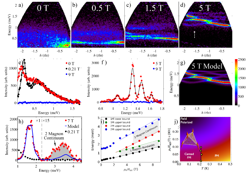
Figure 1: (a-d) Evolution of the magnetic excitation spectrum in [001] magnetic field at 0.15 K. Horizontal axis is the in-plane wavevector component along (100). d) The sharp modes at 5 T can be well described in (g) by spin waves of the model Hamiltonian (1,2). Vertical white arrow shows direction along which intensity is plotted in f) for $h=[-1.8,-1.4]$, fitted to Gaussians (solid line). h) Energy scan showing the two-magnon scattering continuum (shaded area) at 7 T ($E_{i}=6.3$ meV, $h=[-4,0]$, intensities above 2.3 meV (vertical dashed line) are scaled $\times 15$ for visibility). Solid line is the spin-wave prediction for non-interacting magnons. All calculations include the magnetic form factor and convolution with an estimated resolution lineshape. i) Boundaries of the two-magnon (2M) continuum and one-magnon (1M) extreme energies as a function of $\mu_{0}H_{\rm int}$ field, lines are spin-wave calculations, which predict overlap below 2.25 T. b-c) At 0.5 and 1.5 T the highest-energy magnon has merged with the continuum and the three low-energy magnons have strongly renormalized (suppressed) dispersion. a) In zero field a broad scattering continuum dominates, with lineshape shown in e) (red symbols, $h=[-2.1,0]$, lines are guides to the eye. Filled blue circles illustrate quality of the background subtraction and black symbols show that small fields 0.21 T stabilize a sharp mode at low energies. j) Phase diagram showing the canted ferromagnet (FM), paramagnetic (PM) and field-polarized regions, smooth color variation indicates crossovers and filled circles are sharp peaks in heat capacity. Thick arrows show moment directions for a primitive tetrahedron in the canted FM order with the magnetic field applied vertically up.

The spin dynamics in a 6.3 g single crystal of Yb₂Ti₂O₇ were probed using the neutron spectrometer LET Bewley et al. (2011) at the ISIS neutron source, at a temperature of $0.15$ K and in magnetic fields up to 9 T along the [001] axis (for more details see sm ). An estimated non-magnetic background was subtracted from the raw neutron data and intensities were corrected for absorption effects. Unless explicitly stated otherwise, field values quoted throughout refer to the externally applied fields $\mu_{0}H_{\rm app}$, whereas the spin-wave calculations are performed for the corresponding demagnetization-corrected (internal) fields $\mu_{0}H_{\rm int}$ sm . We first discuss the results in high field where the spectrum is dominated by strongly dispersive modes. Fig. 1d) shows representative data at 5 T collected with neutrons of incident energy $E_{i}=2.5$ meV for a fixed sample orientation that probed the scattering at low energies for wavevectors near ($\bar{2}00$). Sharp modes are observed, and a representative lineshape profile is shown in Fig. 1f), which reveals four well-defined peaks, whose positions were extracted using Gaussian fits (solid line). By fitting similar energy scans extracted from a volume of data collected for multiple sample orientations an extensive data set on the dispersion relations was obtained for many reciprocal space directions (shown in Figs. S2 and S3 panels a-d) and m-p) in the Supplemental Material sm ).

The observed sharp modes are physically attributed to magnons originating on the four sublattices of the pyrochlore structure, which can be regarded as an FCC Bravais lattice of corner-shared tetrahedra. Following Ross et al. (2011) we compare the observed dispersion relations to spin-wave modes of a nearest-neighbor Hamiltonian with four symmetry-allowed, anisotropic exchange terms and two $g$-tensor terms ($g_{\parallel}$ and $g_{\perp}$, along and transverse to the local three-fold $\langle 111\rangle$ axes) to describe the Zeeman interaction. The exchange Hamiltonian reads Ross et al. (2011)

$${\cal H}_{\rm Exchange} = \sum_{\langle ij\rangle}\big{\{}J_{zz}\mathsf{S}^{z}_{i}\mathsf{S}^{z}_{j}-J_{\pm}\left(\mathsf{S}^{+}_{i}\mathsf{S}^{-}_{j}+\mathsf{S}^{-}_{i}\mathsf{S}^{+}_{j}\right)$$ (1)

$$+ J_{\pm\pm}\left(\gamma_{ij}\mathsf{S}^{+}_{i}\mathsf{S}^{+}_{j}+\gamma_{ij}^{*}\mathsf{S}^{-}_{i}\mathsf{S}^{-}_{j}\right)$$

$$+ J_{z\pm}\left[\mathsf{S}^{z}_{i}\left(\zeta_{ij}\mathsf{S}^{+}_{j}+\zeta_{ij}^{*}\mathsf{S}^{-}_{i}\right)+\left(i\leftrightarrow j\right)\right]\big{\}},$$

where the sum extends over all nearest-neighbor $ij$ pairs counted once ($\gamma$ and $\zeta$ are geometric terms given in sm ). $\mathsf{S}$ denotes a spin-1/2 operator with components expressed in a local frame where the $z$-axes point along the local [111] direction. Following Ross et al. (2011) we calculate the spin-wave spectrum at high fields after finding the mean-field ground state numerically. Varying any of the six parameters separately ($J_{zz},J_{\pm},J_{\pm\pm},J_{z\pm},g_{\parallel},g_{\perp}$) modifies the equilibrium spin orientation, this affects the spin-wave expansion of the Hamiltonian and in turn the dispersion relations, with the consequence that the parameters are all strongly coupled making it challenging to obtain the values independently in an unbiased way. Strongly coupled parameters generically occur when the spin Hamiltonian does not have rotational symmetry around the field axis, as is the case here not . To provide enough constraints we have extracted over 550 dispersion points combined from our data in field along $[001]$ and previous data in field along $[\bar{1}10]$ from Ross et al. (2011) (the two data sets provide complementary projections of the $g$-tensor and exchange matrices) and also magnetization data near saturation (this further constrains the absolute $g$-values). Using this extended data set a free fit to the six parameters converged to a unique solution (for details see sm )

$$J_{zz}= ~{}0.026(3)~{}{\rm meV}, J_{\pm\pm}=0.048(2)~{}{\rm meV},$$

$$J_{\pm}= ~{}0.074(2)~{}{\rm meV}, J_{z\pm}=-0.159(2)~{}{\rm meV},$$

$$g_{\parallel}= \!\!\!\!\!\!2.14(3), ~{}~{}g_{\perp}=4.17(2).$$ (2)

We find one dominant coupling, the “transverse” exchange $J_{z\pm}$, all other exchanges are much smaller. As a consistency check of the applicability of the spin-wave approximation we have verified that the dispersions at 5 and 9 T are described by the same parameters. This confirms that 5 T is a sufficiently high field that dispersion renormalization effects beyond linear spin wave order are negligible. The above Hamiltonian provides an excellent description of all the data available (compare Figs. 1d and g), Figs. S2 and S3 panels a-d) with e-h) sm . The earlier exchange parameters proposed in Ross et al. (2011), deduced assuming a larger $g$-tensor anisotropy, did not fit the [001] field data well [compare Fig. S2a-d) with i-l)]. The revised parameters fit well the dispersions data for both field directions, and furthermore reproduce THz data on the zone-centre magnon energies at high field [see Fig. S7] and the most recent estimate of the $g$-tensor anisotropy $g_{\perp}/g_{\parallel}$ deduced from crystal-field studies Gaudet et al. (2015); the exchange parameters are also consistent with a recent parameterization of the zero-field quasielastic diffuse scattering pattern at higher temperature (0.4 K)Robert et al. (2015). A semi-classical analysis of this Hamiltonian puts the system in a canted ferromagnetic phase, as seen experimentally. However, the system is located very close in parameter space to a phase boundary with an ordered XY phase sm . This fact may prove to be of significance Jaubert et al. (2015) in understanding the anomalously large fluctuation effects at low field (discussed below).

The INS data in high field contains, in addition to sharp one-magnon modes, also a weak scattering continuum in an energy range corresponding to twice the one-magnon energies. This is illustrated in Fig. 1h) at 7 T. The strong signal in the range 1.3-2.2 meV is due to one-magnon excitations. Note the broad signal in the range 2.75-4 meV, not present at low field (filled circles, 0.21 T). The magnetic character of this continuum scattering is confirmed by a strong field dependence, its energy boundaries move in magnetic field at twice the rate compared to the extreme energies of one-magnon states [see Fig. 1i)] and its integrated intensity increases strongly upon decreasing field [see Fig. S11]. Those features are characteristic for two-magnon excitations. If the Hamiltonian does not have rotational invariance around the field as is the case here, then zero-point quantum fluctuations are present at all fields and reduce the ordered moment from its maximum value and magnetization saturation is reached only asymptotically (as shown in Fig. S19). In the presence of such zero-point fluctuations neutrons can also scatter by simultaneously creating two magnons that share the energy and momentum transfer, thus appearing as a continuum contribution in the INS. Upon lowering the field zero-point quantum fluctuations are expected to grow, the magnetization to decrease and the two-magnon scattering intensity to increase, as indeed observed. Having established the physical origin of the continuum scattering we note that its intensity is underestimated compared to one-magnon states and there is more intensity at the lower boundary than predicted by a non-interacting spin-wave model (solid line in Fig. 1h), implying that magnon-magnon interactions are important for describing the lineshapes quantitatively.

Upon decreasing field the one-magnon energies decrease linearly and the two-magnon continuum boundaries decrease at twice that rate, see Fig. 1i). Qualitative changes in the spectrum occur when the highest-energy magnon branch overlaps with the continuum, expected to occur near 2.25 T. Fig. 1c) shows data well below this field at 1.5 T, the highest-energy magnon can no longer be distinguished from the continuum (suggesting strong one$\rightarrow$two-magnon decay processes) and the dispersion bandwidth of the lower three modes is strongly renormalized (suppressed), suggesting strong interactions between one and two-magnon states even when overlap does not occur. Upon further lowering the field to 0.5 T, Fig. 1b), the three sharp modes appear squeezed into a single, gapped, almost dispersionless branch followed by strong continuum scattering at higher energies At 0.21 T a clear gapped sharp mode can still be observed near 0.22 meV [see Fig. 1e) black circles], and at zero field (red symbols) there is a relatively broad maximum near 0.15 meV and a continuum lineshape extending up to $1.5$ meV. Such dramatic quasi-particle breakdown effects over a large part of the Brillouin zone are very unusual in three-dimensional ordered magnets and demonstrate anomalously strong quantum fluctuations.

To obtain complementary information on the lowest-energy magnetic excitations and evolution of the spin gap in magnetic field we have performed AC heat capacity measurements down to 0.1 K and fields up to 1.5 T $\parallel$ [001] on a 9.7 mg rectangular single crystal (for details see sm ). In zero field, a sharp anomaly is observed near 0.214(2) K [see Fig. 2 top trace, blue symbols]. This anomaly is attributed Chang et al. (2012) to the transition to canted ferromagnetic order with spontaneous ferromagnetic polarization along a cubic axis. We observe that in a very small applied field of 0.05 T (green trace) the anomaly is significantly reduced and a broad hump appears at higher temperatures near 0.25 K. Increasing the field to 0.1 T (cyan trace) the anomaly is almost completely suppressed and has disappeared at 0.125 T, where only a broad Schottky feature is observed, which moves to higher temperature upon increasing the field. Plotting the location of the sharp anomaly on a field-temperature phase diagram in Fig. 1j) shows that the phase transition from paramagnet to the low-temperature canted ferromagnet exists only over a very small field range, above which no phase transition boundary exists. This can be naturally understood as follows. The transition to the canted ferromagnet spontaneously picks the direction of the ferromagnetic polarization along one of the cubic axes (6 domains) and the canting of moments is uniquely determined for each site in relation to the orientation of the local 3-fold axes. In an external magnetic field along [001], the direction of the ferromagnetic polarization is picked by the field $--$ the paramagnet and the ordered phase have the same symmetry $--$ so there is no longer a need for a phase transition. If the transition in zero field were continuous, one would expect it to occur only at strictly zero field. If it were first order, as is believed to be the case here, one would expect it to survive for a small, but finite field range, which is fully consistent with our data. The phase diagram in Fig. 1j) shows that in [001] field the canted ferromagnet and the high-field-polarized state are continuously connected, without encountering a phase transition. This is further supported by the field dependence of the heat capacity data. The strong suppression of heat capacity at low temperatures and presence of a Schottky anomaly that moves to higher temperatures upon increasing field are characteristic signatures of a spin gap that increases monotonically upon increasing field. To parameterize this behavior we have compared the rising part of the $C(T)$ data (up to the broad peak) to the form expected for a two-level system (for details of fits see sm ). The extracted gap is plotted in Fig. 2(inset) and shows a rapid increase in field. The monotonic gap increase is consistent with no phase boundary between the canted ferromagnet and the high-field-polarized state in Fig. 1j).

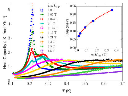
Figure 2: Heat capacity as a function of temperature, $C(T)$, at various fields $\parallel$ [001], vertical dashed line at $T_{\rm N}$ is a guide to the eye. (inset) Gap extracted from the heat capacity data as described in the text, dashed line is guide to the eye.

To summarize, we have reported high-resolution INS measurements of the spin dynamics as a function of applied magnetic field in the frustrated pyrochlore Yb₂Ti₂O₇. We have observed direct evidence for coherent quantum fluctuations manifested in a field-dependent two-magnon scattering continuum at high fields, and strong magnon decay and dispersion renormalization effects at low fields. Through fits to an extensive data set of the high-field magnon dispersions and magnetization data we have re-evaluated the spin Hamiltonian finding dominant quantum exchange terms, which we propose are responsible for the anomalously strong quantum fluctuation effects observed at low field. It may be the case that those effects may be understood as being related to the close proximity of the material to the semi-classical phase boundary between canted ferromagnet and an order-by-disorder antiferromagnet, or potentially a quantum spin liquid phase. We propose that the experimental strategy employed here of probing quasi-particle breakdown in fields comparable to the exchange strength will be a useful experimental tool in future studies of quantum spin liquid candidates. Our results emphasize the need for theoretical efforts to understand the quantum phase diagram of effective spin-1/2 pyrochlore Hamiltonians away from the well-understood semiclassical limit.

JDT was supported by the University of Oxford Clarendon Fund Scholarship and NSERC of Canada. PAM acknowledges support from an STFC Keeley-Rutherford fellowship. Work in Oxford was partially supported by EPSRC (UK) through grants No. EP/H014934/1 and EP/M020517/1.

I Supplemental Material

Here we provide additional technical details on 1) the anisotropic spin exchange Hamiltonian on the pyrochlore lattice, 2) the linear spin-wave formalism to derive the magnon dispersion relations at high fields, 3) time-of-flight inelastic neutron scattering (INS) experiments to probe the spin dynamics, 4) the fitting procedure to extract the Hamiltonian parameters from high-field one-magnon dispersion relations and magnetization, and comparison with THz data, 5) semiclassical calculations for the fitted Hamiltonian: mean-field ordering temperature, Curie-Weiss temperature, mean-field phase diagram, proximity of Yb₂Ti₂O₇ to the phase boundary between canted ferromagnetic and antiferromagnetic orders, 6) observation of a two-magnon scattering continuum at high field and comparison with spin-wave predictions, 7) magnon dispersion renormalization and decay effects when one- and two-magnon phase spaces overlap, 8) ac heat capacity measurements and spin gap dependence in field, 9) magnetization measurements.

II S1. Spin Hamiltonian

II.1 Pyrochlore Lattice and Local Frame

The pyrochlore lattice may be viewed as an FCC Bravais lattice with a tetrahedral basis. The basis is taken to be $\bm{r}_{1}=(a/8)(1,1,1)$, $\bm{r}_{2}=(a/8)(1,-1,-1)$, $\bm{r}_{3}=(a/8)(-1,1,-1)$, $\bm{r}_{4}=(a/8)(-1,-1,1)$ with coordinates given in the global (cubic axes) frame, where $a$ is the cubic lattice parameter. A general site on the pyrochlore lattice labelled $i$ is located at position $\bm{R}_{i}+\bm{r}_{n}$, where $\bm{R}_{i}$ is the FCC lattice position and $n=1$ to $4$ is the sublattice index. A natural choice of coordinate frame on the pyrochlore lattice has the local $z$ axis at each site along the local $[111]$ direction, distinguished by the local oxygen environment. In particular, we take the local right-handed frames for the four sublattices with unit vectors as

$$\bm{\hat{z}}_{1} =\frac{1}{\sqrt{3}}(1,1,1),~{}~{}~{}\bm{\hat{z}}_{2} =\frac{1}{\sqrt{3}}(1,-1,-1)$$

$$\bm{\hat{z}}_{3} =\frac{1}{\sqrt{3}}(-1,1,-1),~{}~{}~{}\bm{\hat{z}}_{4} =\frac{1}{\sqrt{3}}(-1,-1,1)$$ (S1)

and

$$\bm{\hat{x}}_{1} =\frac{1}{\sqrt{6}}(-2,1,1),~{}~{}~{}\bm{\hat{x}}_{2} =\frac{1}{\sqrt{6}}(-2,-1,-1)$$

$$\bm{\hat{x}}_{3} =\frac{1}{\sqrt{6}}(2,1,-1),~{}~{}~{}\bm{\hat{x}}_{4} =\frac{1}{\sqrt{6}}(2,-1,1).$$ (S2)

We define a set of rotation matrices to transform vector components from the global frame to those in the local frame of each sublattice as $R_{n}^{x\beta}=\bm{\hat{x}}_{n}\cdot\bm{\hat{e}}_{\beta}$, $R_{n}^{y\beta}=\bm{\hat{y}}_{n}\cdot\bm{\hat{e}}_{\beta}$, $R_{n}^{z\beta}=\bm{\hat{z}}_{n}\cdot\bm{\hat{e}}_{\beta}$. Here $\bm{\hat{e}}_{\beta}$ stands for a unit vector axis of the global frame, $\beta=x,y$ or $z$.

II.2 Anisotropic Exchange Couplings

The most general, symmetry-allowed exchange matrix between nearest-neighbor spins on the pyrochlore lattice is uniquely defined by four independent terms McClarty et al. (2009); Thompson et al. (2011); Ross et al. (2011); Onoda and Tanaka (2011). Following Ref. Ross et al. (2011) the exchange Hamiltonian expressed in the local frames has the form in (1) where

$$\zeta=\left(\begin{array}[]{cccc}0&-1&e^{i\pi/3}&e^{-i\pi/3}\\ -1&0&e^{-i\pi/3}&e^{i\pi/3}\\ e^{i\pi/3}&e^{-i\pi/3}&0&-1\\ e^{-i\pi/3}&e^{i\pi/3}&-1&0\end{array}\right)$$

and $\gamma=-\zeta^{*}$. In a more abbreviated notation, ${\cal H}_{\rm Exchange}=\sum_{\langle ij\rangle}\mathcal{J}_{ij}^{\alpha\beta}\mathsf{S}^{\alpha}_{i}\mathsf{S}^{\beta}_{j}$ where throughout we use the notation convention that repeated axes indices are summed over. The spin operators are understood to operate on the effective spin one-half doublet at each magnetic site that characterizes the ground state of the crystal field split $J=7/2$ multiplet of the Kramers Yb³⁺ ions. We may neglect the influence of excited crystal field levels because the crystal field gap to the first excited level far exceeds the exchange coupling strengths Gaudet et al. (2015). We neglect the long-range dipolar interaction because it is small compared to the exchange. The quality of our fits (presented below) is such that we do not require the inclusion of exchange couplings beyond nearest neighbor.

The total Hamiltonian including the Zeeman coupling to an external magnetic field is

$${\cal H}={\cal H}_{\rm Exchange}+{\cal H}_{\rm Zeeman}$$ (S3)

with

$${\cal H}_{\rm Zeeman}=-\mu_{\rm B}\mu_{0}H_{\rm int}^{\mu}\sum_{i}g^{\mu\nu}_{n}\mathsf{S}_{i}^{\nu},$$ (S4)

where the magnetic field components $\mu_{0}H_{\rm int}^{\mu}$ are given in the global frame and $g_{n}^{\mu\nu}$ is the $g$-tensor for sublattice $n$.

III S2. Spin Wave Theory

Starting from the spin Hamiltonian with effective spin one-half moments in (S3), we first compute the ground state in a $[001]$ applied magnetic field within mean field theory, assuming that the magnetic structure can always be described using the primitive tetrahedral structural cell (magnetic propagation vector $\bm{q}=\bm{0}$), as is the case semiclassically at both zero and very large fields. The orientation of the effective spin one-half moments within the ground state ${\bm{\hat{u}}}_{n}$ allows us to specify a local quantization frame on each sublattice, where $\bm{\hat{\tilde{z}}}_{n}={\bm{\hat{u}}}_{n}$, $\bm{\hat{\tilde{x}}}_{n}={\bm{\hat{u}}}_{n}\times[1,1,1]/\parallel{\bm{\hat{u}}}_{n}\times[1,1,1]\parallel$ and $\bm{\hat{\tilde{y}}}_{n}=\bm{\hat{\tilde{z}}}_{n}\times\bm{\hat{\tilde{x}}}_{n}$. In addition to the rotation matrices $R_{n}^{\alpha\beta}$ defined above, which rotate from the global to the local frame, rotations from the local frame to the quantization frame are given by $\bar{R}_{n}^{\mu\alpha}$ where $\mu$ is the quantization frame index, $\alpha$ is the local frame index and $n$ is the sublattice label.

In the local quantization frame, we write the spin operators in terms of Holstein-Primakoff (HP) bosons and expand around the classical ground state in powers of $1/S$.

$$\tilde{\mathsf{S}}^{z}_{i} =S-a^{\dagger}_{i}a_{i}$$

$$\tilde{\mathsf{S}}^{+}_{i} =\tilde{\mathsf{S}}^{x}_{i}+i\tilde{\mathsf{S}}^{y}_{i}=\sqrt{2S-a^{\dagger}_{i}a_{i}}a_{i}\approx\sqrt{2S}a_{i}$$

$$\tilde{\mathsf{S}}^{-}_{i} =\tilde{\mathsf{S}}^{x}_{i}-i\tilde{\mathsf{S}}^{y}_{i}=a_{i}^{\dagger}\sqrt{2S-a^{\dagger}_{i}a_{i}}\approx\sqrt{2S}a_{i}^{\dagger}.$$

The commutation relations satisfied by the boson operators are

$$\left[a_{i},a_{j}^{\dagger}\right]=\delta_{ij}.$$

Other commutators vanish.

The leading term in this expansion is the classical Hamiltonian

$$\mathcal{H}_{0}=S(S+1)\sum_{\langle ij\rangle}\mathcal{J}_{ij}^{\alpha\beta}u_{n}^{\alpha}u_{n^{\prime}}^{\beta},$$

where the subscripts $n$ and $n^{\prime}$ are the sublattice indices of the $i$ and $j$ sites, respectively. Here the term of order $S^{2}$ is the mean-field exchange energy and the term of order $S$ comes from symmetrizing the exchange Hamiltonian quadratic in the boson operators.

We write the boson operators in Fourier space. The interaction matrix is then

$$\mathcal{J}_{nn^{\prime}\bm{k}}^{\alpha\beta}=\frac{1}{N}\sum_{ij}\mathcal{J}_{ij}^{\alpha\beta}\exp\left[i\bm{k}\cdot(\bm{R}_{i}-\bm{R}_{j}+\bm{r}_{n}-\bm{r}_{n^{\prime}})\right],$$

where $N$ is the number of FCC lattice sites. In the quantization frame, the interaction matrix becomes $\tilde{\mathcal{J}}_{nn^{\prime}\bm{k}}^{\mu\nu}=\bar{R}_{n}^{\mu\alpha}\bar{R}_{n^{\prime}}^{\nu\beta}\mathcal{J}_{nn^{\prime}\bm{k}}^{\alpha\beta}$.

The terms linear in the bosons vanish in the ground state computed from the minimum semiclassical energy and fluctuations around the ground state may be computed from the quadratic Hamiltonian $\mathcal{H}_{2}$. We introduce operators

$$\bm{\sigma}^{x}_{\bm{k}}\equiv\sqrt{\frac{S}{2}}\left(\bm{a}_{\bm{k}}+\bm{a}^{\dagger}_{-\bm{k}}\right)$$

$$\bm{\sigma}^{y}_{\bm{k}}\equiv i\sqrt{\frac{S}{2}}\left(\bm{a}_{\bm{k}}-\bm{a}^{\dagger}_{-\bm{k}}\right)$$

with $\bm{a}_{\bm{k}}=(a_{1\bm{k}},a_{2\bm{k}},a_{3\bm{k}},a_{4\bm{k}})$ so that

$$\mathcal{H}_{2} =\sum_{\bm{k}}\left(\begin{array}[]{cc}(\bm{\sigma}^{x}_{\bm{k}})^{\dagger}&(\bm{\sigma}^{y}_{\bm{k}})^{\dagger}\end{array}\right)\left(\begin{array}[]{cc}\bm{P}^{x}_{\bm{k}}&\bm{T}_{\bm{k}}\\ \bm{T}^{\star}_{\bm{k}}&\bm{P}^{y}_{\bm{k}}\end{array}\right)\left(\begin{array}[]{c}\bm{\sigma}_{\bm{k}}^{x}\\ \bm{\sigma}_{\bm{k}}^{y}\end{array}\right),$$ (S10)

$$\equiv\sum_{\bm{k}}\left(\begin{array}[]{cc}(\bm{\sigma}^{x}_{\bm{k}})^{\dagger}&(\bm{\sigma}^{y}_{\bm{k}})^{\dagger}\end{array}\right)\boldsymbol{H}\left(\begin{array}[]{c}\bm{\sigma}_{\bm{k}}^{x}\\ \bm{\sigma}_{\bm{k}}^{y}\end{array}\right),$$ (S14)

where the sum runs over all wavevectors $\bm{k}$ in the first Brillouin zone of the FCC lattice and where

$$P^{x}_{nn^{\prime}\bm{k}} =\mathcal{R}_{n}\delta_{nn^{\prime}}+\tilde{\mathcal{J}}_{nn^{\prime}\bm{k}}^{xx}+\frac{\mu_{\rm B}}{2}\mu_{0}H_{\rm int}^{\alpha}R_{n}^{\beta\alpha}g^{\beta}\bar{R}_{n}^{z\beta}\delta_{nn^{\prime}}$$

$$P^{y}_{nn^{\prime}\bm{k}} =\mathcal{R}_{n}\delta_{nn^{\prime}}+\tilde{\mathcal{J}}_{nn^{\prime}\bm{k}}^{yy}+\frac{\mu_{\rm B}}{2}\mu_{0}H_{\rm int}^{\alpha}R_{n}^{\beta\alpha}g^{\beta}\bar{R}_{n}^{z\beta}\delta_{nn^{\prime}}$$

$$T_{nn^{\prime}\bm{k}} =\tilde{\mathcal{J}}_{nn^{\prime}\bm{k}}^{xy}$$

and $\mathcal{R}_{n}=-\sum_{n^{\prime}}\tilde{\mathcal{J}}_{nn^{\prime},\bm{k}=\bm{0}}^{zz}$. Since the $g$-tensor is diagonal in the local frame, with the form $g={\rm diag}(g_{\perp},g_{\perp},g_{\parallel})$, we write $g$ with a single index denoting the diagonal element.

The diagonalization of the quadratic Hamiltonian $\mathcal{H}_{2}$ in (S14) to find the magnon wavefunctions and energies must preserve the boson commutation relations, which take the form

$$\left[\bm{\sigma}_{\bm{k}}^{\alpha},\left(\bm{\sigma}_{\bm{k}}^{\beta}\right)^{\dagger}\right]=S\bm{\eta}^{\alpha\beta}$$

with

$$\bm{\eta}\equiv\left(\begin{array}[]{cc}0&-i\bm{I}\\ i\bm{I}&0\end{array}\right),$$

where $\bm{I}$ is the $4\times 4$ identity matrix. Then the spin wave energies $\omega_{m\bm{k}}$ for modes $m=1$ to 4 are the positive semidefinite set of eigenvalues of the matrix $2\bm{\eta H}$ and the right eigenvectors $\bm{v}_{m\bm{k}}$ of $\bm{\eta H}$ preserve the commutation relation among the $\bm{\sigma}$ operators provided that $\bm{v}^{\dagger}\bm{\eta}\bm{v}=\bm{g}$, where $\bm{g}={\rm diag}(1,1,1,1,-1,-1,-1,-1)$.

The neutron scattering intensity is proportional to

$$\left|F(\bm{Q})\right|^{2}\sum_{\alpha,\beta}\left(\delta_{\alpha\beta}-\hat{Q}_{\alpha}\hat{Q}_{\beta}\right)S^{\alpha\beta}\left(\bm{Q},\omega\right),$$

where $\bm{Q}=\bm{k}_{i}-\bm{k}_{f}$ is the wavevector transfer, $\bm{k}_{i}$ ($\bm{k}_{f}$) is the incident (final) neutron wavevector, $\omega$ is the neutron energy transfer and $F(\bm{Q})$ is the magnetic form factor of Yb³⁺ ions, assumed spherically symmetric. The indices $\alpha$ and $\beta$ are components of the moments in the global frame. We evaluate the inelastic part of the scattering function at zero temperature

$$S^{\alpha\beta}_{\rm inelas}\left(\bm{Q},\omega\right)=$$

$$~{}~{}~{}~{}\sum_{n,n^{\prime}}\sum_{E}\langle 0|\mathsf{J}^{\alpha}_{n}(-\bm{Q})|E\rangle\langle E|\mathsf{J}^{\beta}_{n^{\prime}}(\bm{Q})|0\rangle\delta\left(\omega-\omega_{E}\right),$$ (S15)

where the second sum is over all excited states $|E\rangle$ of energy $\omega_{E}$ above the ground state $|0\rangle$. The physical moment $\mathsf{J}^{\alpha}_{n}$ is related to the effective spin one-half moment components in the quantization frame $\tilde{\mathsf{S}}_{n}^{\gamma}$ through $\mathsf{J}^{\alpha}_{n}=\Gamma_{n}^{\alpha\gamma}\tilde{\mathsf{S}}^{\gamma}_{n}$ where we have defined $\Gamma_{n}^{\alpha\gamma}\equiv R_{n}^{\beta\alpha}g^{\beta}\bar{R}_{n}^{\gamma\beta}$.

One-magnon excited states are accessed via spin fluctuations with transverse polarization ($\mu,\nu=x$ or $y$) in the quantization frame, and the corresponding inelastic scattering function is

$$S^{\alpha\beta}_{\rm inelas,1M} \left(\bm{Q},\omega\right)=\frac{S}{2}\sum_{n,n^{\prime}}\sum_{\mu\nu=x,y}\Gamma_{n}^{\alpha\mu}\Gamma_{n^{\prime}}^{\beta\nu}\times$$

$$\sum_{m}v^{\mu\dagger}_{mn,-\bm{k}}v^{\nu}_{mn^{\prime}\bm{k}}e^{-i\bm{\tau}\cdot\bm{r}_{nn^{\prime}}}\delta(\omega-\omega_{m\bm{k}}),$$ (S16)

where $\bm{r}_{nn^{\prime}}=\bm{r}_{n}-\bm{r}_{n^{\prime}}$ and the eigenvectors are written as $v^{\mu}_{mn\bm{k}}$, indexed by the transverse spin deviation component $\mu=x,y$. Here $\bm{k}$ is the wavevector transfer reduced to the first Brillouin zone, i.e. $\bm{Q}=\bm{\tau}+\bm{k}$ where $\bm{\tau}$ is closest reciprocal lattice vector to $\bm{Q}$.

Two-magnon excited states are accessed via fluctuations polarized longitudinally in the quantization frame. To see this we consider the longitudinal scattering function for the effective spin in the quantization frame, which has an analogous form to (S15)

$$S_{{\rm eff},nn^{\prime}}^{zz}(\bm{Q},\omega)\equiv\sum_{E}\langle 0|\tilde{\mathsf{S}}^{z}_{n}(-\bm{Q})|E\rangle\langle E|\tilde{\mathsf{S}}^{z}_{n^{\prime}}(\bm{Q})|0\rangle\delta(\omega-\omega_{E}),$$ (S17)

where

$$\tilde{\mathsf{S}}^{z}_{n}(\bm{Q}) =\sqrt{N}S\delta(\bm{k})e^{-i\bm{\tau}\cdot\bm{r}_{n}}$$

$$-\frac{1}{\sqrt{N}}\sum_{\bm{q},\bm{q^{\prime}}}\delta(\bm{k}-\bm{q}+\bm{q^{\prime}})a_{n\bm{q}}^{\dagger}a_{n\bm{q^{\prime}}}e^{-i\bm{\tau}\cdot\bm{r}_{n}}$$ (S18)

is the component of the effective spin along the quantization direction. The first term leads to a contribution of to order $S^{2}$ in the structure factor (S17), which is the elastic, Bragg scattering in the ordered phase. The second term in (S18) leads to an inelastic contribution of order $S^{0}$ in the structure factor (S17), due to magnon pair creation/annihilation.

We introduce

$$\Lambda_{mn\boldsymbol{q}} \equiv(v^{x}_{mn\boldsymbol{q}}-iv^{y}_{mn\boldsymbol{q}})/2$$

$$\bar{\Lambda}_{mn\boldsymbol{q}} \equiv(v^{x}_{mn\boldsymbol{q}}+iv^{y}_{mn\boldsymbol{q}})/2.$$ (S19)

It is also convenient to introduce $\Omega_{\bm{q}\bm{q^{\prime}}nmm^{\prime}}\equiv\Lambda_{mn\bm{q}}\bar{\Lambda}_{m^{\prime}n\bm{q^{\prime}}}+\bar{\Lambda}_{mn\bm{q}}\Lambda_{m^{\prime}n\bm{q^{\prime}}}(1-(2-\sqrt{2})\delta_{mm^{\prime}}\delta(\bm{q^{\prime}}-\bm{q}))$ such that the inelastic part of (S17) becomes

$$S {}_{{\rm eff,inelas},nn^{\prime}}^{zz}(\bm{Q},\omega)=\frac{1}{N}\sum_{\bm{q},\bm{q^{\prime}}}\sum_{m\geq m^{\prime}}\Omega^{\star}_{\bm{q}\bm{q^{\prime}}nmm^{\prime}}\Omega_{\bm{q}\bm{q^{\prime}}n^{\prime}mm^{\prime}}\times$$

$$~{}~{}~{}~{}~{}e^{-i\bm{\tau}\cdot\bm{r}_{nn^{\prime}}}\delta(\bm{k}-\bm{q}-\bm{q^{\prime}})\delta\left(\omega-\omega_{m\bm{q}}-\omega_{m^{\prime}\bm{q^{\prime}}}\right).$$

The two-magnon scattering from the physical moment is given by

$$S^{\alpha\beta}_{\rm inelas,2M}\left(\bm{Q},\omega\right)=\sum_{n,n^{\prime}}\Gamma_{n}^{\alpha z}\Gamma_{n^{\prime}}^{\beta z}S_{{\rm eff,inelas},nn^{\prime}}^{zz}(\bm{Q},\omega),$$

which we have evaluated numerically using a Monte Carlo integration over the Brillouin zone in order to compare with the experimental data.

IV S3. Inelastic Neutron Scattering Experiments

IV.1 Experimental Details

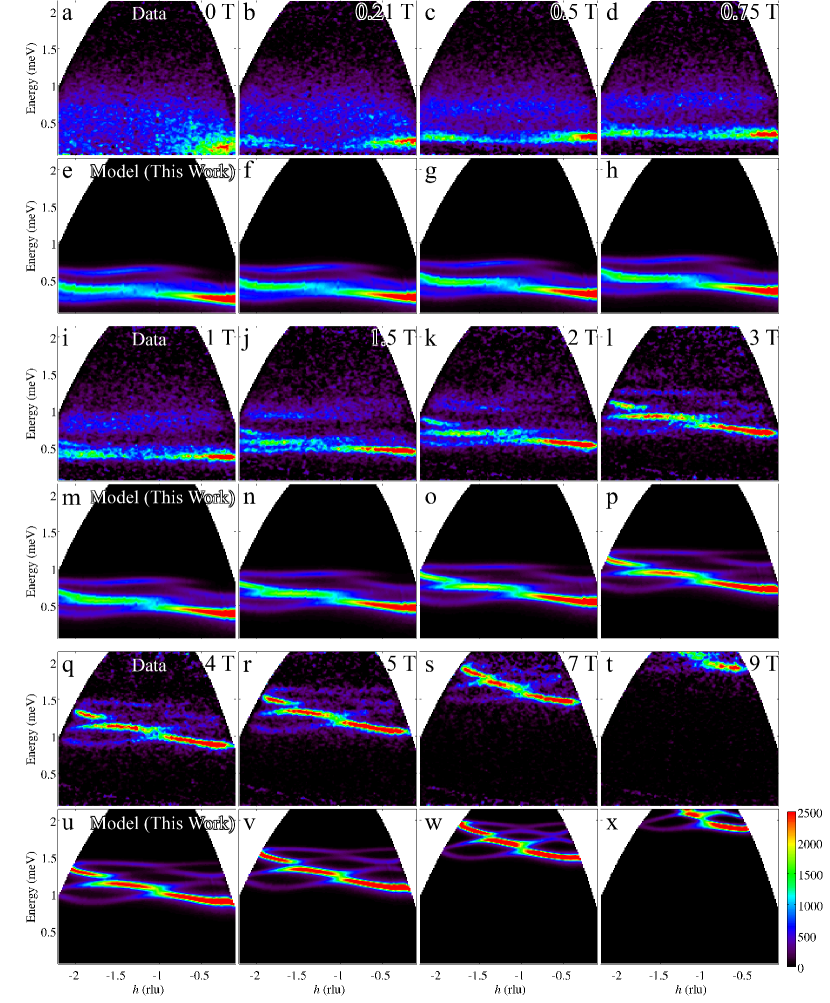
Figure S1: Overview of the spin dynamics as a function of field along $[001]$. The top panel and every other subsequent row of panels shows raw data, paired with the corresponding spin-wave calculation for the model Hamiltonian. The data was collected for $E_{i}=2.5$ meV and horizontal axis shows the in-plane wavevector component along the (100) direction (intensities are averaged for the vertical component in the range $l=[-0.5,0.5]$). Calculations are performed for the estimated internal fields in Table S3 and include the magnetic form factor and convolution with an estimated resolution lineshape.

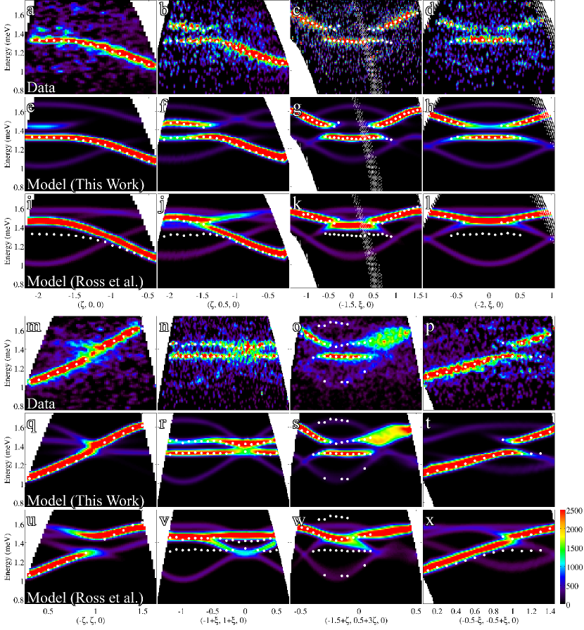
Figure S2: Representative dispersion maps at 5 T $\parallel[001]$ along various directions in the ($hk0$) plane (red lines in Fig. S4). Panels (a-d,m-p) show experimental data ($E_{i}=2.5$ meV), the row of panels immediately below (e-h,q-t) show the corresponding spin wave calculation for the model Hamiltonian in (2), whereas the subsequent row of panels (i-l,u-x) show the calculation for the model in Ref. Ross et al. (2011). The white solid dots show the location of experimentally-extracted dispersion points, determined by fitting Gaussian peaks to energy scans at constant wavevector. Calculations are performed for a demagnetization-corrected field $\mu_{0}H_{\rm int}=4.93$ T and include the magnetic form factor and convolution with an estimated energy resolution. Intensities are averaged for transverse wavevectors in the range $l,k=[-0.2,0.2]$ for the ($h00$) direction, and similar ranges for the other directions.

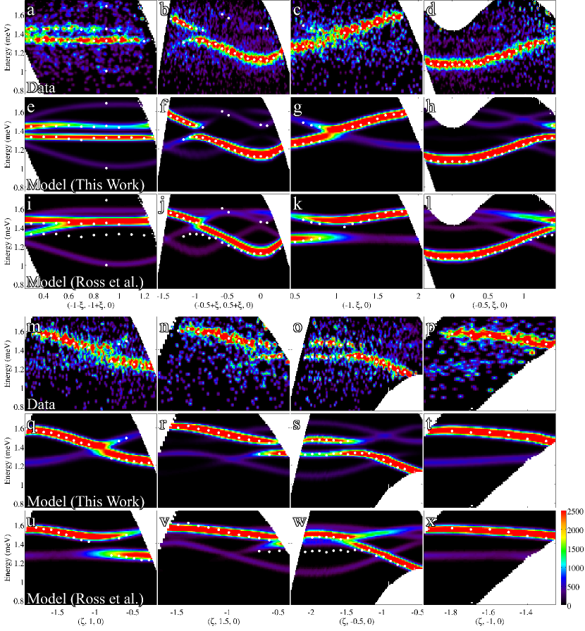
Figure S3: Same as Fig. S2, but for other directions in the ($hk0$) plane.

A single crystal of Yb₂Ti₂O₇ was grown as described in Ref. Prabhakaran and Boothroyd (2011) using a four-mirror optical floating-zone furnace (Crystal System Inc.) in an argon rich atmosphere with a growth rate of 1-2 mm/h, similar to the conditions reported in Ref. Chang et al. (2012). Due to the argon atmosphere, the as-grown crystal was oxygen deficient and dark in color. In order to improve the oxygen stoichiometry, the as-grown crystal was annealed at 1200^∘C for 5 days under oxygen flow atmosphere and the crystal become transparent and almost colorless. Several pieces were cut from this larger crystal and used for all the different measurements reported here.

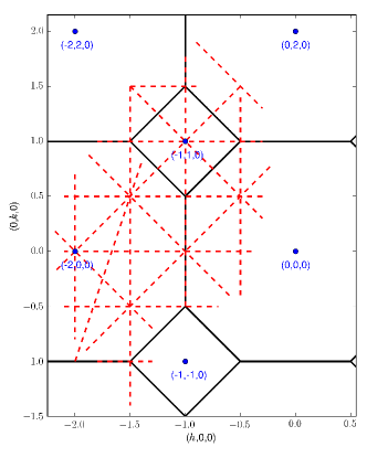
Figure S4: Schematic of the ($hk0$) horizontal scattering plane indicating where dispersion maps were extracted from Horace scans (red lines) and plotted in Figs. S2 and S3 panels a-d) and m-p). Solid black lines show intersections with the FCC Brillouin zone boundaries.

The spin dynamics was probed using the direct-geometry time-of-flight chopper spectrometer LET at the ISIS neutron source Bewley et al. (2011) using a cylindrical-shaped $6.3$ g single crystal of Yb₂Ti₂O₇ aligned in the $(hk0)$ horizontal scattering plane. The sample was cooled using a dilution fridge insert with a base temperature of 0.15 K where all measurements were performed, this temperature is well below the zero-field magnetic ordering transition temperature of 0.214(2) K [see phase diagram in Fig. 1j)]. Magnetic fields up to 9 T were applied along the crystal [001] axis using a vertical cryomagnet. Applied fields were corrected for demagnetization effects as discussed in Sec. S9. To avoid complexities associated with multiple (ferro)magnetic domains the sample was cooled to base temperature in a finite magnetic field (0.21 T) to ensure a single magnetic domain with ferromagnetic polarization along the field. The zero-field data was collected last, after reducing the field to zero from finite values. The inelastic scattering was probed for neutrons with incident energy $E_{i}=1.34$, $2.5$, 4 and $6.3$ meV, with measured energy resolutions of $0.023(1)$, $0.055(2)$, $0.094(1)$ and $0.220(5)$ meV (Full Width Half Maximum), respectively, on the elastic line. For the majority of the measurements LET was operated in multi-repetition mode, allowing the mapping of the inelastic scattering with $E_{i}=1.34$, 2.5 and 6.3 meV simultaneously. For an overview of how the spin dynamics evolves as a function of field, measurements were performed up to 9 T for a fixed sample orientation that probed the scattering at low energies for wavevectors near ($\bar{2}00$), with a typical counting time of $2.5$ h per setting; those results are summarized in Fig. S1 (top and every other subsequent row). To obtain an extended data set on the wavevector-dependence of the spin dynamics in the Brillouin zone the inelastic scattering was measured at a selection of fixed applied fields (0, 0.21, 1.5 and 5 T) for a range of sample rotation angles around the vertical [001] direction spanning $90^{\circ}$ in steps of $1^{\circ}$ (Horace scan), each position counted for approximately $7$ minutes. This gave access to a wide range of wavevectors in the ($hk0$) plane and typical intensity maps extracted from this data volume are shown in Fig. S2a-d). We estimated the non-magnetic energy-dependent background using Fig. 1i) as a guide to indicate where no magnetic scattering is expected at different fields, i.e. at high fields no magnetic signal is expected below the one-magnon gap and in the interval between the one- and two-magnon energy ranges (shaded regions in Fig. 1i), whereas at low field no magnetic signal is expected at very high energies. The estimated non-magnetic background was subtracted from the raw intensities to obtain the purely magnetic signal, which was afterwards corrected for neutron absorption effects using a numerical Monte Carlo routine for a tilted cylindrical sample (assuming an inverse velocity dependence of the neutron absorption cross-section). Throughout this paper, wavevectors are given as $(h,k,l)$ in reciprocal lattice units of $2\pi/a$ of the structural cubic unit cell with lattice parameter $a=10.026$ Å Gardner et al. (2004).

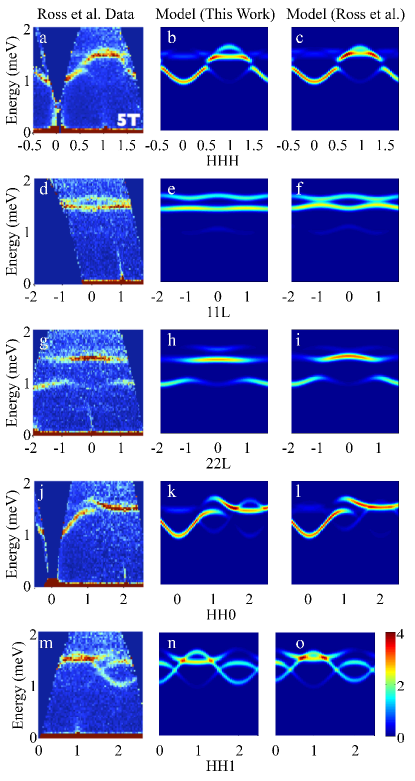
Figure S5: Dispersion maps along various directions in the ($hhl$) plane for a field of 5 T along [$\bar{1}10$] (first column is INS data from Ross et al. (2011)), compared with spin-wave calculations for the refined Hamiltonian in (2)(middle column) and the model in Ref Ross et al. (2011). Both calculations include the magnetic form factor and convolution with a finite energy resolution of 0.09 meV (FWHM). Spin-wave calculations using the applied field value of 5 T or an estimated demagnetization-corrected field of $\mu_{0}H_{\rm int}=4.93$ T gave essentially indistinguishable results (the latter is plotted in the figure).

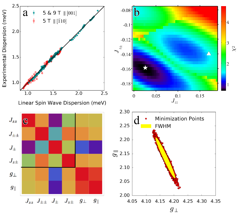
Figure S6: a) Agreement between experimental and calculated spin-wave energies for the fitted Hamiltonian in (2). The graph contains over 550 data points, filled cyan symbols correspond to fields of $5$ and $9$ T $\parallel[001]$ and red open circles to field of $5$ T $\parallel[\bar{1}10]$, the latter from from Ross et al. (2011). The solid line corresponds to perfect agreement. b) Map of the goodness of fit ($\chi^{2}$) as a function of $J_{zz}$ and $J_{z\pm}$, where for each point the remaining (four) Hamiltonian parameters are freely optimized against all data points in a) and the magnetization constraint. The location of the optimal parameter set (2) is indicated by the white star in the middle of the dark region (global minimum). The white triangle (middle of right-hand side) corresponds to the parameter values in Ref. Ross et al. (2011). c) Absolute value of the correlation coefficient between the six fitted parameters. d) Visual illustration of the correlation between $g_{\parallel}$ and $g_{\perp}$, red dots illustrate the parameter values when the experimentally-determined spin-wave energies are randomly shifted within their errorbars, yellow elliptical contour shows the half-maximum contour of this distribution.

IV.2 High-field Spin-wave Dispersions

Representative intensity maps for some high-symmetry directions in the ($hk0$) plane are shown in Figs. S2 and S3 panels a-d) and m-p). In those figures the row of panels immediately below the raw data, e-h) and q-t), are the spin-wave calculation for the fitted Hamiltonian (2), and demonstrate an excellent agreement with the data along all directions probed. For comparison, the subsequent row of panels, i-l) and u-x), show the calculation for the parameters in Ref. Ross et al. (2011), in this case systematic differences are seen in terms of shifts of the dispersion modes between the data and the model predictions, compare for example Fig. S2a-d) with i-l), from which we conclude that the earlier proposed model cannot account for the observed dispersions in field along [$001$], whereas the current refined model can account for all the dispersion data, even for field along [$\bar{1}10$], see Fig. S5.

IV.3 S4. Fitting Procedure to Determine the Spin Hamiltonian

In this section we give details of the fitting procedure used to obtain the Hamiltonian parameters from experimentally measured magnon dispersion relations at high fields. From the INS data in applied fields of $5$ and $9$ T $\parallel[001]$ we extracted energy scans [as in Fig. 1e)] and determined mode energies $\omega_{m}$, where the subscript $m=1$ to 4 labels the modes at a given ($h,k,l$) in order of increasing energy. For some scans it was not possible to detect four distinct modes, but by continuity with neighboring regions in reciprocal space, we were able to determine the appropriate labels of all the visible modes. This way we obtained a list of dispersion points $(h,k,l,\omega,m)$. In order to provide multiple and independent constraints on the fits, we also extracted dispersion points from the INS data reported in Ross et al. (2011) in a field of $5$ T$\parallel[\bar{1}10]$. We also included in the fitting procedure the requirement for the model to reproduce the measured magnetization value at $\mu_{0}H_{\rm int}=6.86$ T $\parallel$ [001], at which field the magnetization is almost saturated (see Sec. S9).

By computing the magnon dispersion relations within linear spin wave theory, we carried out a least squares minimization allowing all six parameters of the Hamiltonian to vary independently. The minimization was based on a simulated annealing algorithm that was run several thousand times, initialized every time with different random starting parameters, for an extensive sampling of the parameter space to detect the global minimum.

As a first test, we fixed the $g$ tensor ratio $g_{\perp}/g_{\parallel}=2.4$ as in Ross et al. (2011) and the minimization procedure using only the $[\bar{1}10]$ dispersion data set converged, within error, to the parameter values given in that paper. We also found that the $5$ T$\parallel[001]$ dispersions data alone were insufficiently constraining to determine both $g$ factor elements. In other words, the minimization procedure on this data set alone, without a constraint on the $g$-factor components leads to almost degenerate solutions with different sets of parameters. However, by taking the $5$ T$\parallel[\bar{1}10]$ dispersion data, and the $5$ and $9$ T $\parallel[001]$ dispersions data sets, together with the $7$ T$\parallel[001]$ magnetization, we obtained a unique, optimum solution, with a clear global minimum in the goodness of fit, that can account for all the data. We emphasize that when not all the neutron data and magnetization constraints are included in the fitting procedure, there is a family of almost degenerate solutions to the optimization problem.

The existence of a set of parameters that nearly satisfy all the fitting constraints is a consequence of the strong correlation between certain parameters. In Fig. S6d), we show the magnitude of the correlation coefficient between the six parameters. All $6$ parameters are significantly correlated with particularly large correlations between the two $g$ factor parameters, which can be traced back to the constraint on the magnetization. In the absence of the magnetization constraint, the strongest correlation is between $J_{zz}$ and $g_{\parallel}$.

The refined Hamiltonian parameters obtained using all the above mentioned data points are given in (2), where the quoted uncertainties were estimated as follows. Each dispersion point ($h,k,l,w,m$) had an energy uncertainty $\sigma$, which ranged between $0.01$ and $0.02$ meV. The larger error bars are for the magnon energies determined visually from the digitized INS intensity maps reported in Ref. Ross et al. (2011). We created a list of $10^{4}$ sets of mode energies, where each set is shifted from the original by a gaussian random number times the standard deviation of the energy of that mode. We carried out the least square minimization to determine the optimum model parameters for each such set of slightly shifted mode energies. The errors on the model parameters were then extracted from the resulting distributions of those fitted parameters.

Field Misalignment $-$ In the INS measurements the magnetic field was slightly misaligned relative to the $[001]$ crystallographic axis by $1.0(1)^{\circ}$. We have verified that assuming perfect alignment $\parallel[001]$ or including this small misalignment resulted in essentially identical values for the optimized parameters, within the uncertainties listed in (2).

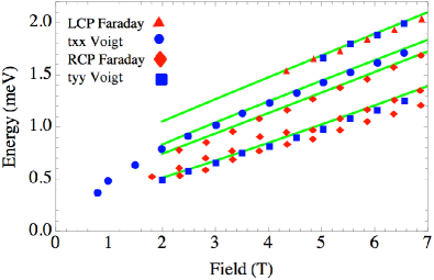
Figure S7: THz spectrum as a function of magnetic field along [001] from Ref. Pan et al. (2014), symbols correspond to excitation energies observed using different experimental geometries and polarizations as listed in the legend. Solid lines are the calculated spin-wave energies at the zone center, $\omega_{1-4,\bm{k}=\bm{0}}$, for the model Hamiltonian in (2), assuming quoted field values have negligible demagnetization corrections.

IV.4 Comparison with THz data

As a further test of the determined Hamiltonian we have verified consistency also with the recently reported THz spectrum for field $\parallel[001]$. THz spectroscopy measures the long wavelength ($\bm{k}=\bm{0}$) excitation spectrum and in total four main families of peaks are observed using different experimental setups, see Fig. S7. The energies of the observed modes are well reproduced (solid lines) for fields above 3 T by the spin wave energies calculated for the Hamiltonian in (2) with no adjustable parameters. At lower fields linear spin wave theory fails owing to the proximity of single and two-magnon states (as discussed later in Sec. S7).

We have also verified the applicability of the THz selection rules to the observation of spin wave modes. THz spectroscopy measures the complex transmittance $t(\omega)$ of initially polarized THz radiation through a single crystal sample in the presence of a static magnetic field. The transmittance is proportional to the imaginary part of the susceptibility $\chi^{\prime\prime}_{\alpha\beta}(\omega)$, which we calculate using a random phase approximation. The Faraday geometry with the incident THz pulse in the $z$ direction and linearly polarized in the $x$ direction and the Voigt geometry with the field in the $y$ direction, where all axes labels refer to the global (cubic axes) frame. In the case of the Faraday geometry, Ref. Pan et al. (2014) concentrated on the transmittance of circularly polarized radiation. We find that the spectrum in the Voigt geometry, obtained from $\chi^{\prime\prime}_{xx}(\omega)$ and $\chi^{\prime\prime}_{yy}(\omega)$, is sensitive to three magnon modes - the lowest and two highest modes, as indeed observed (blue symbols in Fig. S7). In the Faraday geometry, the lowest mode should appear in the right circularly polarized channel, from $\chi^{\prime\prime}_{xx}(\omega)-\chi^{\prime}_{xy}(\omega)$, and the highest mode in the left circularly polarized channel, $\chi^{\prime\prime}_{xx}(\omega)+\chi^{\prime}_{xy}(\omega)$. However, the second-to-lowest mode should not be visible using the Faraday geometry although, apparently, this mode is visible in the data. However, if we allow for a small field misalignment away from the $[001]$ direction then the second-to-lowest mode exhibits a peak in the THz spectrum, making the Faraday spectrum also consistent with the model predictions.

V S5. Semiclassical Properties of the Spin Hamiltonian

V.1 Quantum Fluctuations

The role of quantum fluctuations on the size of the ordered moment may be computed within linear spin wave theory. The departure of the effective spin one-half moment from its fully available value $S=1/2$ is given by

$$\Delta S\equiv\frac{1}{4N}\sum_{i}\langle a_{i}^{\dagger}a_{i}\rangle=\frac{1}{4N}\sum_{\bm{k}}\sum_{n,m}{\Lambda}^{*}_{mn\bm{k}}{\Lambda}_{mn\bm{k}}$$ (S20)

in terms of the rotated eigenvectors $\Lambda$, defined in (S19). At 5 T we obtain a relatively small reduction of 2%, providing at least a partial consistency check to justify the applicability of the linear spin-wave approach to parameterize the dispersion relations and extract the Hamiltonian. We note however that even though quantum fluctuations are small at those fields, they are still present and are ultimately responsible for the observation of a weak, but finite intensity two-magnon continuum in addition to the dominant one-magnon excitations in INS (to be discussed in detail in Sec. S6).

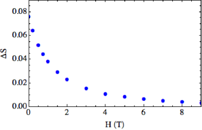
Figure S8: Spin reduction $\Delta S$ as a function of applied field calculated using linear spin-wave theory, eq. (S20).

V.2 Total Moment Sum Rule

The total moment sum rule is a single constraint on the structure factor computed for a model with spin $S$

$$\frac{1}{N}\sum_{\bm{k},\alpha}\int S_{\rm eff}^{\alpha\alpha}(\bm{k},\omega)~{}d\omega=S(S+1)$$ (S21)

where the structure factor $S_{\rm eff}$ is computed for the effective spin one-half moment. This is to be distinguished from the experimental structure factor for Yb₂Ti₂O₇, which is computed for the true $\mathsf{J}$ moment in the ground state crystal field doublet.

In this section, we compile various contributions to the total scattering sum rule for the exchange parameters determined from experiment. We concentrate on the 9 T magnon spectrum because, of all the measured fields, this one should be the closest match to linear spin wave theory. In the previous section we discussed the leading order quantum correction to the ordered spin, which is $\Delta S=0.0030$ at 9 T. The total elastic, one- and two-magnon contributions are listed in Table S1. The combined total differs from the sum rule in (S21) by less than 0.25%, such small violations of the sum rule are generally expected in linear spin wave theory, higher order contributions in $1/S$ are generally needed to renormalize the intensities to agree with the sum rules.

Table S1: Calculated contributions to total (effective spin) sum rule at $9$ T. The elastic (Bragg) contribution is $(S-\Delta S)^{2}$ where $\Delta S$ is the zero-point spin reduction in (S20). The single magnon (1M) and two magnon (2M) contributions are obtained from numerical integration of the transverse and longitudinal (effective spin) dynamical correlations, respectively.

	Elastic	1M	2M	Total
Intensity	0.241	0.50244	0.0051	0.74854

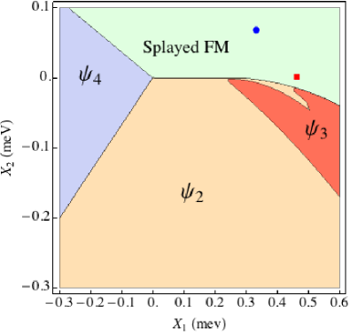
Figure S9: Semiclassical phase diagram in the space of anisotropic exchange parameters given in Eq. (1). The origin of the phase diagram is a Coulomb phase at the classical level. Three long-ranged ordered phases appear in its vicinity: a splayed (canted) ferromagnet (FM) with spontaneous polarization along one of the cubic directions, the $\psi_{4}$(Palmer-Chalker) McClarty et al. (2009) antiferromagnetic state and a ground state with an accidental degeneracy in the $\Gamma_{5}$ manifold, resolved by quantum fluctuations into long-range ordered antiferromagnetic states $\psi_{2}$ (as in the ordered phase of Er₂Ti₂O₇) or $\psi_{3}$, both with only a discrete degeneracy McClarty et al. (2009). All these phases have ordering wavevector $\bm{q}=\bm{0}$. Two points are marked on the phase diagram corresponding to the exchange values proposed by Ross et al. Ross et al. (2011) (blue circle) and those obtained here (red square). The $X_{1}$ and $X_{2}$ coordinates are linear combinations of the primary couplings chosen such that the phase diagram includes both sets of Hamiltonian parameters and also the Coulomb phase at the origin. In particular, $X_{1}=\left\{-0.9198,-0.3834,-0.084,0\right\}$ and $X_{2}=\left\{0.349,-0.7233,-0.5204,0.2904\right\}$ in the space of couplings $\left\{J_{zz},J_{\pm\pm},J_{\pm},J_{z\pm}\right\}$.

V.3 Mean-Field Phase Diagram

The fit to the exchange parameters fixes the semiclassical ground state of Yb₂Ti₂O₇ to be a canted ferromagnet with an ordering wavevector $\bm{q}=\bm{0}$ and spontaneously chosen net polarization along one of the cubic axes. The moments are non-collinear, tilted towards the the local [111] axes. The mean field $T_{c}\approx 2.95$ K is far in excess of the observed transition temperature in the material. We have computed the ground state phase diagram for the exchange model Eq. (1) in the vicinity of these exchange parameters in order to point out proximate phases. To this purpose, we choose a highly symmetric point in the space of anisotropic couplings that harbors a Coulomb phase at the classical level corresponding to couplings $J_{zz}=1$, $J_{\pm\pm}=0.5$, $J_{\pm}=0.25$ and $J_{z\pm}=-1/\sqrt{8}$ Benton et al. (2016). We rescale these couplings so that $J_{z\pm}$ matches the value extracted from the experimental data namely $-0.162$ meV. Then we choose to plot the phase diagram in Fig. S9 in a plane through the space of couplings containing both the exchange values proposed by Ross et al. Ross et al. (2011) (blue circle) and those obtained here (red square). Evidently, both sets of parameters place Yb₂Ti₂O₇ in the same phase, which is the same as the one determined experimentally. The principal difference between the two sets of exchange parameters is that the set determined in this work lies very close to the phase boundary with the $\psi_{3}$ state with antiferromagnetic order. While apparent from the phase diagram, one may confirm that the difference between the mean field energy of the ground state and the energy of the $\psi_{3}$ state is smaller for the exchange parameters determined in this work.

V.4 Curie-Weiss Temperature

The Curie-Weiss temperature obtained from a high temperature expansion for the Hamiltonian in (S3) is Ross et al. (2011)

$$2k_{\rm B}(2g_{\perp}^{2}+g^{2}_{\parallel})\Theta_{\rm CW}$$

$$=\left(g_{\parallel}^{2}J_{\rm{zz}}-4g_{\perp}^{2}\left(J_{\pm}+2J_{\pm\pm}\right)-8\sqrt{2}g_{\perp}g_{\parallel}J_{z\pm}\right).$$

For the parameters in Ref. Ross et al. (2011), $\Theta_{\rm CW}=312$ mK whereas we find $641$ mK for the parameters extracted in this study. This calculated value is to be compared with experimental values of $400$ mK Blöte et al. (1969) and $750$ mK Hodges et al. (2001).

V.5 Magnon Decay Matrix Element

The spin structure of Yb₂Ti₂O₇ is noncollinear for the entire range of fields explored in the experiment reported here. Then, in the local quantization frame there are terms for an isotropic exchange Hamiltonian that couple $x$ and $z$ components of the spins. As a consequence, the $1/S$ expansion in terms of Holstein-Primakoff (HP) bosons contains cubic interaction terms which take one magnon into two or vice versa. In our case, such terms arise as a consequence of noncollinearity and anisotropic exchange in the global frame.

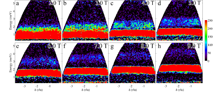
Figure S10: INS data collected in a high-flux and low neutron absorption configuration ($E_{i}=6.3$ meV) to maximize the sensitivity to observe the weak two-magnon continuum scattering. The strong (out-of-range) signal at intermediate energies is due to one-magnon excitations, the weaker intensity band of scattering at higher energies is due to two-magnon excitations. Note the continuum scattering increases in intensity and moves to lower energies upon decreasing field. An energy scan through the 7 T data is shown in Fig. 1h).

The spin wave dispersions, computed to quadratic order in HP bosons, are renormalized by interaction terms. In the case of cubic terms, there is a self-energy contribution $\boldsymbol{\Sigma}\left(\bm{k},\omega_{\bm{k}}\right)$ to the spectrum coming from bubble diagrams. Schematically

$$\boldsymbol{\Sigma}\left(\bm{k},\omega_{\bm{k}}\right)\sim\sum_{\bm{q}}\frac{|\Gamma\left(\bm{k},\bm{q}\right)|^{2}}{\omega_{\bm{k}}-\omega_{\bm{q}}-\omega_{\bm{k}-\bm{q}}+i0^{+}}$$

where $\Gamma$ is the amplitude of the cubic vertex and for clarity we have omitted the individual mode labels of the three magnon energies, which in principle can each belong to a different dispersion mode $m$. There are singularities in the integrand whenever the single magnon energy $\omega_{\bm{k}}$ overlaps with the two-magnon continuum $\omega_{\bm{q}}+\omega_{\bm{k}-\bm{q}}$. When this is the case, magnon decay processes become kinematically allowed and one expects a renormalization of the spectrum and also magnons acquire a finite lifetime resulting in a broadening of the magnon peaks at the nominal energy $\omega_{\bm{k}}$. The extent of these effects depends strongly on the density of states of two magnon decays. In Yb₂Ti₂O₇ the estimated threshold field below which the two-magnon continuum overlaps with the highest-energy one-magnon dispersion mode is $2.3$ T and below this field experiments observe a substantial broadening of the highest energy magnon lineshape in the overlap region (see Sec. S7).

VI S6. Two-Magnon Scattering Continuum at High Fields

The INS intensity maps at high field showed a distinct continuum intensity signal at energies corresponding to twice the one-magnon energies, identified with neutrons scattering by creating a pair of magnons. The intensity map in Fig. S10e) shows this scattering contribution at 6 T, note the weak band of scattering intensity centered around 3 meV, which shifts in energy upon varying field (compare with data in panels at other fields). Energy scans observing directly the shift in energy and intensity increase upon lowering field are shown in Fig. S11a) (shaded areas).

A quantitative comparison with spin-wave theory for non-interacting magnons in Fig. 1h)(solid line) shows that the intensity of the continuum scattering relative to the one-magnon intensity is underestimated, and also that the continuum lineshape profile is different (more intensity at the lower boundary), suggesting that inclusion of magnon-magnon interactions may be required to account for those features. Apart from an overall renormalization of the relative continuum intensity its strong increase upon lowering field is well captured by spin-wave theory (solid line) in Fig. S11b). The wavevector-dependence of the continuum intensity at 5 T is shown in Fig. S12a), the intensity has a local minimum near ($\bar{2}00$), and this feature is well captured by the spin-wave prediction for the two-magnon intensity (panel b).

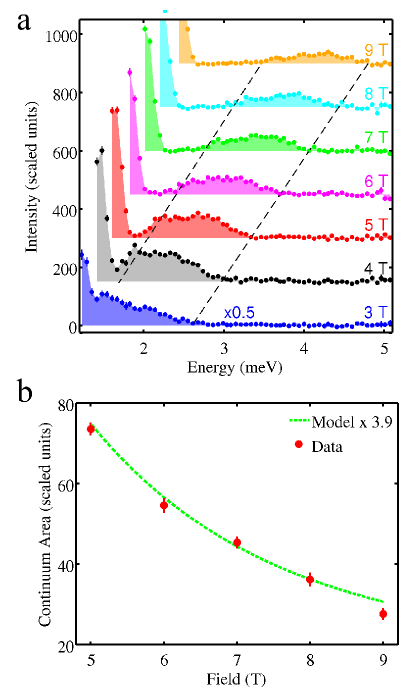
Figure S11: (a) Energy scans through the intensity maps in Fig. S10 ($h=[-4,0]$) showing the two-magnon scattering continuum increasing in intensity and being displaced to lower energies upon decreasing field from top to bottom traces (shading emphasizes the magnetic intensity). For clarity traces are offset vertically (by +150) as a function of increasing field. Dashed lines indicate the linear field dependence of the extracted continuum boundaries. Intensities in the lower trace are multiplied by 0.5 to fit on the same scale. b) Experimentally-extracted energy integrated area of the continuum scattering (from scans such as in Fig. 1h) as a function of internal field and the corresponding spin-wave prediction for two-magnon scattering (solid line) times an overall scaling factor given in the legend.

VII S7. Magnon Decay and Dispersion Renormalization at Intermediate Fields

An overview of the field-dependence of the spin dynamics is plotted in Fig. S1 as a function of increasing field in the top and every other subsequent row, whereas the rows of panels immediately below show the spin-wave calculation. Good agreement is found above $\sim$$3$ T, below this field one- and two-magnon phase spaces overlap [see Fig. 1i)] and more complex behavior occurs. The energy scan in Fig. S13a) at 3 T shows four well-resolved sharp peaks followed by a weak scattering continuum (shaded area) centered near 1.5 meV. Upon lowering field to 2 T (panel b) the lower three peaks have shifted to lower energies, whereas the fourth peak has merged with the continuum with a lower boundary near 1 meV. We interpret this “disappearance” of the highest-energy magnon mode as being due to its spontaneous decay into two-magnon states. Upon lowering the field further to 1.5 T (panel c) the whole pattern shifts to lower energies and furthermore the energy spacing between the lower three peaks is clearly smaller than at 3 T (panel a). At 1 T (d) the peaks 1 and 2 have almost merged and the spacing 1-3 is reduced further. This magnon bandwidth narrowing is not captured by the (linear) spin-wave approach, which predicts almost field-independent bandwidths, compare Fig. S1c-d) with g-h).

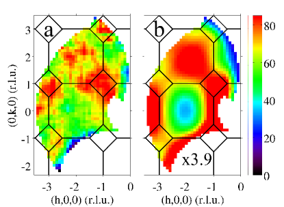
Figure S12: (a) Wavevector-dependence of the continuum scattering intensity in the $(hk0)$ plane at 5 T. Data comes from a Horace scan averaged over $E=[2.03,3.06]$ meV and $l=[-0.2,0.2]$. b) Corresponding intensity map of the two-magnon continuum scattering in spin-wave theory, with the same overall scale factor as in Fig. S11. Solid lines show intersections with the FCC Brillouin zone boundaries.

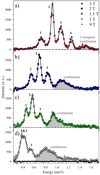
Figure S13: Energy scan illustrating magnon decay and dispersion renormalization effects below the field where one- and two-magnon phase spaces overlap. The spacing between the lowest three sharp modes (labelled 1-3) is significantly reduced as the whole group shifts to lower energies upon reducing field (top to bottom). At the same time the relative separation to the high-energy continuum scattering (shaded area) reduces, at 2 T (panel b) the fourth magnon mode has already “dissolved” in the continuum, which rapidly grows in intensity upon lowering field. Data in all scans comes from the intensity maps at the corresponding fields in Fig. S1 for $h=[-2.2,-1.5]$ and $l=[-0.4,0.4]$. Filled triangles in bottom panel show 9 T data to illustrate the quality of the non-magnetic background subtraction.

We attribute the dispersion renormalization to the increase of quantum fluctuations upon lowering field, also manifested in the continuum intensity now becoming comparable to that of the sharp modes. Physically, a reduction in the magnon bandwidth could be interpreted as a reduction in the kinetic energy that one-spin-flip states gain from coherently hopping across the lattice sites, or an effective inhibition of such coherent propagation due to the increased quantum fluctuations at low field. Given the close proximity between the sharp modes and the continuum boundary at those low fields it may be possible that the dispersion renormalization effects observed might be captured, at least partly, by including interactions between the one-magnon states and the higher-energy continuum scattering.

VII.1 Scattering Continuum in Zero Field

The discrepancy between the linear spin-wave prediction and the data becomes even more dramatic in the region of very low fields. In zero field the spin-wave model predicts sharp modes in the range 0.21-0.61 meV, whereas the data shows a broad scattering continuum throughout this range with considerable scattering weight at lower energies and also extending up to 1.5 meV, compare Fig. S1a and e). The continuum scattering lineshapes are clearly apparent in Fig. 1e) (red symbols) with no clear sharp modes seen in this energy range, in clear contrast with the spin-wave prediction.

An overview of how the spectrum evolves as a function of field for several wavevector directions in the ($hk0$) plane extracted from a Horace data volume is shown in Fig. S14. Notice the contrast between the 5 T data (top row) dominated by well-defined sharp modes with a large gap, and zero field (bottom row) where an extended scattering continuum dominates. At a relatively small applied field of 0.21 T a clear sharp mode is stabilized near 0.22 meV for small $|\bm{Q}|$ see Fig. S14h) (bottom left), but the continuum scattering up to 1.5 meV is essentially unchanged compared to zero field (compare with panel k). Continuum scattering is observed at all wavevectors probed, with some clear intensity modulations illustrated in Fig. S16, the intensity is strongest near the ($hh0$) line for energies below $\sim$0.4 meV (panel a), at higher energies the intensity appears more uniformly distributed (panels b-c). The zero and low field spin dynamics is in sharp contrast with linear spin-wave theory, which would predict a spectrum dominated by dispersive sharp magnon modes, compare Figs. S14 and  S15 (bottom rows). We interpret this dramatic quasiparticle breakdown over a large part of the Brillouin zone as an indication that fluctuations become very strong in the low field regime, presumably due to the dominant “quantum” exchange term $J_{z\pm}$, with the consequence that a semiclassical linear spin-wave description becomes inadequate to capture the spin dynamics.

VIII S8. Heat Capacity Measurements

Heat capacity measurements were collected using a home-made setup based on the AC technique Rost (2010); Sullivan and Seidel (1968). The sample was a flat-plate 9.7 mg single crystal of Yb₂Ti₂O₇ with approximate dimensions $1.85\times 1.61\times 0.45$ mm³ cut from the same piece as the crystal used for the INS measurements. Cooling was provided by an Oxford Instruments Kelvinox25 dilution refrigerator, of base

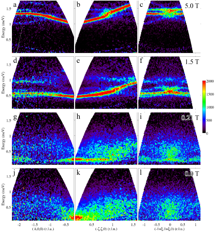
Figure S14: Field-dependence of the excitation spectrum for several high-symmetry directions in the ($hk0$) plane, field decreases from top to bottom. Corresponding spin-wave calculations are shown in Fig. S15. Data was extracted from a Horace scan with $E_{i}=2.5$ meV. Intensities are averaged for transverse wavevectors in the range $l,k=[-0.2,0.2]$ for the ($h00$) direction, and similar ranges for the other directions.

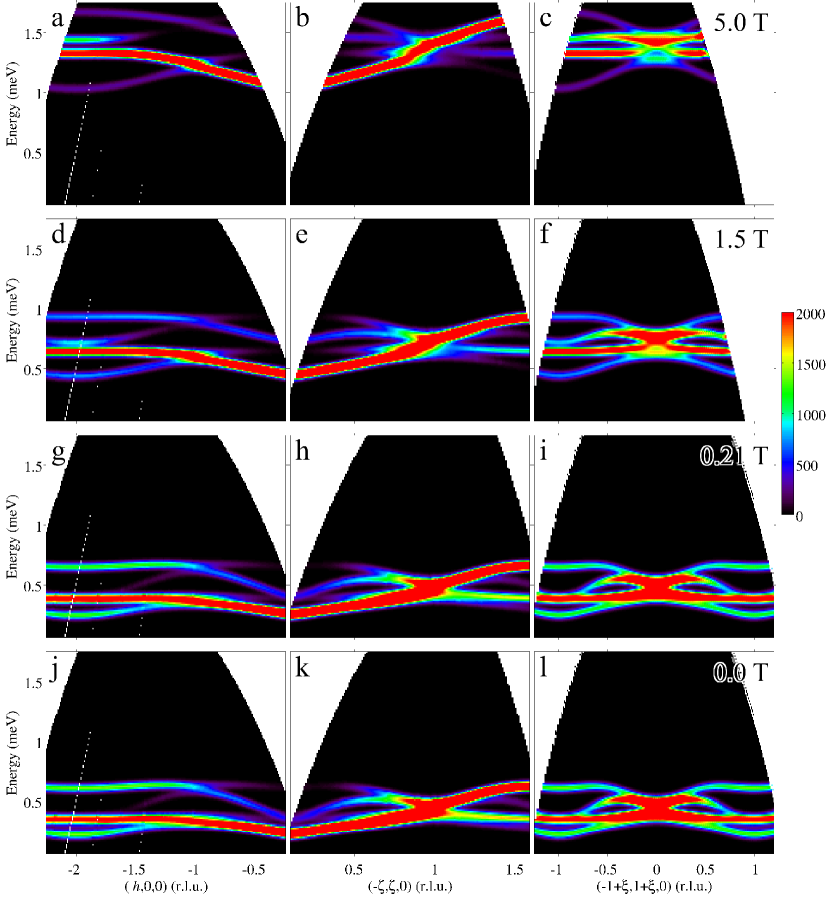
Figure S15: Spin-wave calculations corresponding to the data plotted in Fig. S14. Calculations are performed for demagnetization-corrected fields and include the magnetic form factor and convolution with an estimated energy resolution.

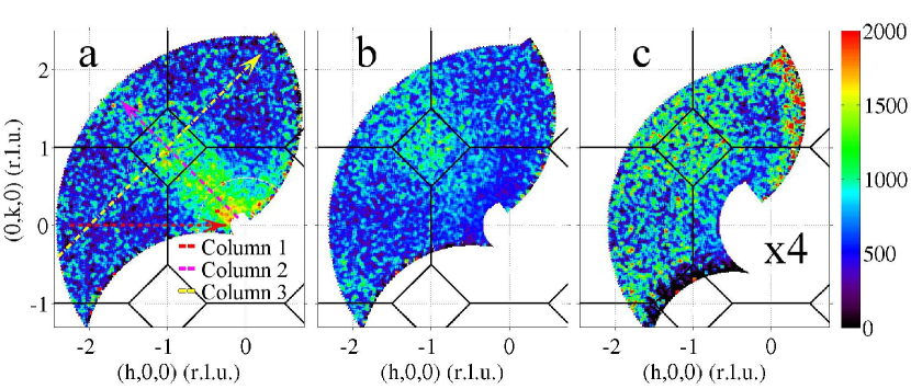
Figure S16: Wavevector-dependence of the zero field continuum scattering intensity in the ($hk0$) plane at a) low ($[0.04,0.4]$ meV), b) intermediate ($[0.4,0.8]$ meV) and c) high energies ($[0.8,1.5]$ meV). Intensities are averaged over transverse wavevectors in the range $l=[-0.2,0.2]$. In panel c) intensities are scaled $\times 4$ to bring them on the same range as the other panels. Solid black lines show intersection with FCC Brillouin zone boundaries. Dashed arrowed lines in a) labelled 1-3 show directions along which the spectrum is plotted in Fig. S14 columns 1-3.

temperature $\sim$$30$ mK, equipped with a $16$ T superconducting magnet, with the sample aligned such that the magnetic field was applied perpendicular to the sample plate, along the [001] crystal direction.

The heat capacity setup contained a Lakeshore RX-$102$A-BR Ruthenium Oxide thermometer mounted on the sample using Apiezon N grease, which was then connected to a $5\times 5\times 0.150$ mm³ $99.95\%$ pure Ag platform. A $120~{}\Omega$ strain gauge was connected to the bottom of the platform using GE $7031$ varnish and used as a heater to apply an oscillating temperature at a frequency of $5\times 10^{-3}$ Hz. A $1$ cm $99.99\%$ pure Pt wire was used to establish a heat link between the platform and an OFHC Copper heat sink connected to the mixing chamber of the dilution fridge. The thermometer was calibrated down to $30$ mK in zero field against a calibrated Lakeshore RX-$102$B-CB thermometer. Field calibrations of the thermometer were performed using constant temperature magnetic field sweeps. The measured heat capacity was normalized into absolute units by calibration against the known specific heat of a standard sample measured in the same setup. The applied magnetic field values $\mu_{0}H_{\rm app}$ were corrected for demagnetization effects to obtain the net internal fields $\mu_{0}H_{\rm int}$ as discussed in Sec. S9.

The heat capacity was measured at fixed applied field as a function of increasing temperature. Fig. S17 displays the obtained heat capacity in zero field (blue symbols). The behavior is comparable to that reported in Ref. Chang et al. (2012) (red symbols) on a crystal where the sharp low-temperature anomaly has been identified with the onset of spontaneous canted ferromagnetic order. Systematic studies of samples of various purities have shown that more stoichiometric samplesRoss et al. (2014); Arpino et al. display a single sharp peak in the heat capacity (at temperatures up to 0.26 K), whereas samples believed to be affected by substantial structural disorder/stuffing/oxygen non-stoichiometry show rather different behavior, with only a broad peak or multiple peaksRoss et al. (2012). The presence of a single sharp peak in the heat capacity of our sample is indicative of a sharp transition to a well-developed magnetic order, suggesting that structural disorder effects are rather small and the magnetic behavior is representative of the high-purity limit.

Fig. 2 shows heat capacity measurements in applied magnetic field. Above $0.1$ T the sharp peak observed in zero field is completely suppressed, replaced by a broad Schottky feature Gopal (1966). Upon increasing field the low-temperature tail of the specific heat is progressively suppressed and the Schottky anomaly moves to higher temperatures, both are indications of a gap in the excitation spectrum, which increases upon increasing field. To capture this trend we compare the data to the behavior expected for a system with an excited level at energy $\Delta$ above the ground state,

$$C(T)=R\left(\frac{\Delta}{k_{\rm B}T}\right)^{2}\frac{e^{-\Delta/k_{\rm B}T}}{\left(1+e^{-\Delta/k_{B}T}\right)^{2}}.$$ (S22)

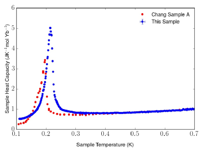
Figure S17: Specific heat as a function of temperature in zero magnetic field (blue symbols) compared to earlier reports Chang et al. (2012) (red symbols).

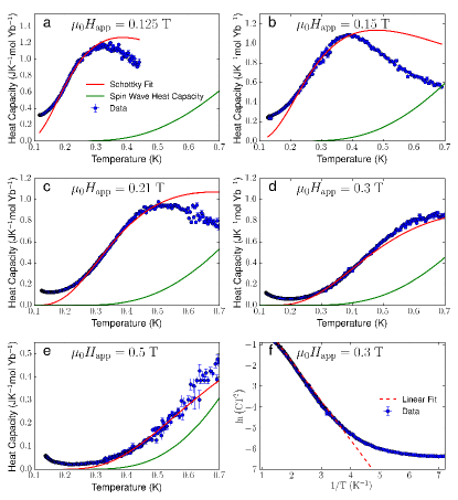
Figure S18: a-e) Specific heat as a function of temperature and magnetic field $\parallel[001]$. Solid lines show fits of the rising part of $C(T)$ to a two-level system, eq. (S22), solid green lines show the spin-wave prediction. Data points are the raw specific heat minus an estimate of the non-magnetic contribution obtained from measurements at high field (lower trace in Fig. 2). f) Same data as in d) plotted now as $\ln\left(CT^{2}\right)$ vs. $1/T$ to expose the near-linear dependence (dashed line) predicted by (S22) for $T\ll\Delta/k_{\rm B}$.

This form was fitted to the measured $C(T,B)$ data in the temperature region up to the broad peak maximum and avoiding the very low-temperature part, where quadrupolar contributions lead to a $1/T^{2}$ behavior, seen already in earlier measurements Blöte et al. (1969). The non-magnetic contribution was estimated from the measured $C(T)$ at high field (lowest trace in Fig. 2) when the spin gap is $\sim$0.4 meV, such that the population of thermally excited magnon states over the whole temperature range of the heat capacity measurements (up to $0.7$ K) is negligible. The fits are illustrated in Fig. S18

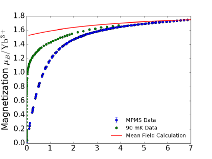
Figure S19: Magnetization as a function of magnetic field along [001] (blue points, 1.8 K). Green points are lower temperature (0.09 K) data from Ref. Lhotel et al. (2014). The red solid line is the zero-temperature mean-field calculation, which reproduces well the observed magnetization value near saturation.

and give a good parameterization of the rising part of $C(T)$. The fitted pre-factor $R$ is systematically lower than the expected molar gas constant, a reduction would be expected as INS measurements [see Fig. 1b)] show a density of states that is not concentrated solely in a single level at the gap energy $\Delta$ as assumed by (S22), but is in fact extended over a wide energy range above the gap. The gap extracted from the heat capacity data is plotted in Fig. 2(inset) and shows a monotonic increase in field.

Table S2: Internal field as a function of applied field for the heat capacity measurements.

$\mu_{0}H_{\rm app}$(T)	$0.05$	$0.075$	$0.1$	$0.125$	$0.15$	$0.21$	$0.30$	$0.5$	$1.5$
$\mu_{0}H_{\rm int}$ (T)	$<0.001$	$0.0013(2)$	$0.007(1)$	$0.019(2)$	$0.035(3)$	$0.084(3)$	$0.165(4)$	$0.354(4)$	$1.330(5)$

Table S3: Internal field (typical uncertainty $\sim$0.002 T) as a function of applied field for the INS measurements.

$\mu_{0}H_{\rm app}$ (T)	$0.21$	$0.5$	$0.75$	$1$	$1.5$	$2$	$3$	$4$	$5$	$6$	$7$	$8$	$9$
$\mu_{0}H_{\rm int}$ (T)	$0.166$	$0.45$	$0.698$	$0.946$	$1.44$	$1.94$	$2.94$	$3.94$	$4.93$	$5.93$	$6.93$	$7.93$	$8.93$

As already shown by the INS data the low-field behavior of the excitations cannot be captured by a spin-wave approach, a scattering continuum dominates instead of sharp modes and moreover there is a large density of states at energies much below the predicted spin-wave gap in zero field of 0.2 meV, compare Fig. S1a) with f). The failure of linear spin-wave theory to capture the low-field behavior is also dramatically illustrated by the specific heat data. Fig. S18a-e) shows that the calculated spin-wave heat capacity $C_{\rm SW}$ (solid green curves) significantly underestimates the low-temperature heat capacity at low fields, as expected if excited states existed below the predicted spin-wave gap. The comparison also shows that upon increasing field the spin-wave calculation becomes progressively closer to the data, this is expected as in the limit of high enough fields where all the low-energy excitations are well-defined, sharp magnons, then we know from comparison to the INS data (at 5 T) that spin-wave theory provides a very good description of the low-energy states, compare Fig. 1d) and g). The comparison in Fig. S18a-e) is consistent with the expectation that $C_{\rm SW}$ approaches the measured $C(T)$ at high enough fields.

IX S9. Magnetization Measurements

Magnetization data was collected in order to provide further constraints on the overall scale of the $g$-tensor. Measurements were performed at 1.8 K using a SQUID magnetometer (Quantum Design MPMS) on a near-rectangular 27.50(2) mg single crystal of Yb₂Ti₂O₇ with approximate dimensions $2.09\times 1.81\times 1.01$ mm³ cut from the same crystal piece used for the heat capacity and INS experiments. The sample was aligned such that the magnetic field was applied normal to the largest sample face, along the $[001]$ crystallographic axis. Fig. S19 shows the obtained magnetization curve, which gives a magnetic moment at the highest field probed of $\mu_{0}H_{\rm int}=6.86$ T of $1.745(4)\mu_{B}$ per Yb³⁺ ion. Field values were corrected for demagnetization effects as discussed below.

IX.1 Demagnetization corrections

The applied magnetic fields in the magnetization, specific heat and neutron scattering measurements were corrected for demagnetization effects to obtain the internal fields $H_{\rm int}=H_{\rm app}-NM$ where $N$ is the demagnetization factor and $M$ is the magnetization volume density. For the heat capacity and magnetization samples $N$ was calculated as $0.64$ and 0.49, respectively, using analytical results for a rectangular prism Chen et al. (2012). The sample used for the INS measurements was a cylinder with the magnetic field applied at an angle $\theta\simeq 32^{\circ}$ to the cylinder axis. Here the internal field was approximated considering only the projection of the demagnetization field along the applied field axis, giving an effective $N\simeq N_{\parallel}\cos^{2}\theta+N_{\perp}\sin^{2}\theta$, where the demagnetization factors for the directions along and transverse to the cylinder axis were calculated as $N_{\parallel}=0.13$ and $N_{\perp}=0.44$, respectively, using analytical results for a cylinder Chen et al. (1991). The estimated internal fields for the heat capacity and neutron data are listed in Tables S2 and  S3, where we used as the reference magnetization curve $M$ vs. $\mu_{0}H_{\rm int}$ the reported data at 90 mK up to 4 T $\parallel[001]$ from Lhotel et al. (2014) supplemented with our own magnetization data extended up to 7 T at 1.8 K [see Fig. S19]. The quoted errors in the tables include an uncertainty in matching the absolute scales of the above two magnetization curves such that the estimated extrapolation of the 90 mK data to high fields overlaps with the 1.8 K data above 5 T. Since the neutron scattering data was collected at a slightly higher temperature of 150 mK where the magnetization is expected to be somewhat reduced compared to 90 mK in the limit of low fields, in the region of low fields the demagnetization corrections are therefore overestimated, so the quoted internal fields in Table S3 are to be interpreted as a lower bound and to become more accurate at high fields where the magnetization is less sensitive to temperature. Similarly, for the heat capacity temperature scans at constant applied field in Fig. 2, the internal fields quoted in Table S2 are to be interpreted as the values at the lowest temperatures at the start of the scans, the actual internal fields are expected to increase towards the applied field value upon increasing temperature (as the magnetization decreases, so demagnetization corrections reduce).

References

- Castelnovo et al. (2012) C. Castelnovo, R. Moessner, and S. L. Sondhi, Annu. Rev. Condens. Matter Phys. 3, 35 (2012).
- Savary et al. (2012) L. Savary, K. A. Ross, B. D. Gaulin, J. P. C. Ruff, and L. Balents, Phys. Rev. Lett. 109, 167201 (2012).
- Zhitomirsky et al. (2012) M. E. Zhitomirsky, M. V. Gvozdikova, P. C. W. Holdsworth, and R. Moessner, Phys. Rev. Lett. 109, 077204 (2012).
- Savary and Balents (2012) L. Savary and L. Balents, Phys. Rev. Lett. 108, 037202 (2012).
- Ross et al. (2014) K. A. Ross, Y. Qiu, J. R. D. Copley, H. A. Dabkowska, and B. D. Gaulin, Phys. Rev. Lett. 112, 057201 (2014).
- Blöte et al. (1969) H. W. J. Blöte, R. F. Wielinga, and W. J. Huiskamp, Physica 43, 549 (1969).
- Yasui et al. (2003) Y. Yasui, M. Soda, S. Iikubo, M. Ito, M. Sato, N. Hamaguchi, T. Matsushita, N. Wada, T. Takeuchi, N. Aso, and K. Kakurai, J. Phys. Soc. Japan 72, 3014 (2003).
- Bonville et al. (2004) P. Bonville, J. A. Hodges, E. Bertin, J.-P. Bouchaud, P. Dalmas De Réotier, L.-P. Regnault, H. M. Rønnow, J.-P. Sanchez, S. Sosin, and A. Yaouanc, Hyperfine Interact. 156, 103 (2004).
- Gardner et al. (2004) J. S. Gardner, G. Ehlers, N. Rosov, R. W. Erwin, and C. Petrovic, Phys. Rev. B 70, 180404 (2004).
- Ross et al. (2009) K. A. Ross, J. P. C. Ruff, C. P. Adams, J. S. Gardner, H. A. Dabkowska, Y. Qiu, J. R. D. Copley, and B. D. Gaulin, Phys. Rev. Lett. 103, 227202 (2009).
- Thompson et al. (2011) J. D. Thompson, P. A. McClarty, H. M. Rønnow, L. P. Regnault, A. Sorge, and M. J. P. Gingras, Phys. Rev. Lett. 106, 187202 (2011).
- Ross et al. (2011) K. A. Ross, L. Savary, B. D. Gaulin, and L. Balents, Phys. Rev. X 1, 021002 (2011).
- Chang et al. (2012) L.-J. Chang, S. Onoda, Y. Su, Y.-J. Kao, K.-D. Tsuei, Y. Yasui, K. Kakurai, and M. R. Lees, Nat. Commun. 3, 992 (2012).
- Ross et al. (2012) K. A. Ross, T. Proffen, H. A. Dabkowska, J. A. Quilliam, L. R. Yaraskavitch, J. B. Kycia, and B. D. Gaulin, Phys. Rev. B 86, 174424 (2012).
- Applegate et al. (2012) R. Applegate, N. R. Hayre, R. R. P. Singh, T. Lin, A. G. R. Day, and M. J. P. Gingras, Phys. Rev. Lett. 109, 097205 (2012).
- Gaudet et al. (2016) J. Gaudet, K. A. Ross, E. Kermarrec, N. P. Butch, G. Ehlers, H. A. Dabkowska, and B. D. Gaulin, Phys. Rev. B 93, 064406 (2016).
- Hayre et al. (2013) N. Hayre, K. Ross, R. Applegate, T. Lin, R. Singh, B. Gaulin, and M. Gingras, Phys. Rev. B 87, 184423 (2013).
- Pan et al. (2014) L. Pan, S. K. Kim, A. Ghosh, C. M. Morris, K. A. Ross, E. Kermarrec, B. D. Gaulin, S. M. Koohpayeh, O. Tchernyshyov, and N. P. Armitage, Nat. Commun. 5, 4970 (2014).
- Lhotel et al. (2014) E. Lhotel, S. R. Giblin, M. R. Lees, G. Balakrishnan, L. J. Chang, and Y. Yasui, Phys. Rev. B 89, 224419 (2014).
- Chang et al. (2014) L.-J. Chang, M. R. Lees, I. Watanabe, A. D. Hillier, Y. Yasui, and S. Onoda, Phys. Rev. B 89, 184416 (2014).
- Gaudet et al. (2015) J. Gaudet, D. D. Maharaj, G. Sala, E. Kermarrec, K. A. Ross, H. A. Dabkowska, A. I. Kolesnikov, G. E. Granroth, and B. D. Gaulin, Phys. Rev. B 92, 134420 (2015).
- Pan et al. (2016) L. Pan, N. J. Laurita, K. A. Ross, E. Kermarrec, B. D. Gaulin, and N. P. Armitage, Nat. Phys. 12, 361 (2016).
- Robert et al. (2015) J. Robert, E. Lhotel, G. Remenyi, S. Sahling, I. Mirebeau, C. Decorse, B. Canals, and S. Petit, Phys. Rev. B 92, 064425 (2015).
- Tokiwa et al. (2016) Y. Tokiwa, T. Yamashita, M. Udagawa, S. Kittaka, T. Sakakibara, D. Terazawa, Y. Shimoyama, T. Terashima, Y. Yasui, T. Shibauchi, and Y. Matsuda, Nat. Commun. 7, 10807 (2016).
- Yaouanc et al. (2016) A. Yaouanc, P. D. de Réotier, L. Keller, B. Roessli, and A. Forget, J. Phys. Condens. Matter 28, 426002 (2016).
- (26) K. E. Arpino, B. A. Trump, A. O. Scheie, T. M. McQueen, and S. M. Koohpayeh, arXiv:1701.08821v1 .
- Bewley et al. (2011) R. I. Bewley, J. W. Taylor, and S. M. Bennington, Nucl. Instr. and Meth. A 637, 128 (2011).
- (28) See Supplemental Material for more technical details of the experiments, data analysis and semi-classical spin-wave and phase diagram calculations.
- (29) For a Hamiltonian with rotational symmetry around the applied field direction, the magnon dispersion relations in the field-polarized phase have a particularly simple form, the sum of independent, linear terms in the -factor and the exchange interactions, therefore the parameters can be directly extracted from dispersions data Coldea et al. (2002). In Yb2Ti2O7 there is no rotational symmetry along any direction, the dispersions at high field are not simple sums of independent terms and the different parameters are strongly coupled in their effect on the dispersions.
- Jaubert et al. (2015) L. Jaubert, O. Benton, J. G. Rau, J. Oitmaa, R. Singh, N. Shannon, and M. J. Gingras, Phys. Rev. Lett. 115, 267208 (2015).
- Coldea et al. (2002) R. Coldea, D. A. Tennant, K. Habicht, P. Smeibidl, C. Wolters, and Z. Tylczynski, Phys. Rev. Lett. 88, 137203 (2002).
- McClarty et al. (2009) P. A. McClarty, S. H. Curnoe, and M. J. P. Gingras, J. Phys. Conf. Ser. 145, 012032 (2009).
- Onoda and Tanaka (2011) S. Onoda and Y. Tanaka, Phys. Rev. B 83, 094411 (2011).
- Prabhakaran and Boothroyd (2011) D. Prabhakaran and A. Boothroyd, J. Cryst. Growth 318, 1053 (2011).
- Benton et al. (2016) O. Benton, L. Jaubert, H. Yan, and N. Shannon, Nat. Commun. 7, 11572 (2016).
- Hodges et al. (2001) J. A. Hodges, P. Bonville, A. Forget, M. Rams, K. Krolas, and G. Dhalenne, J. Phys. Cond. Matt. 13, 9301 (2001).
- Rost (2010) A. W. Rost, Magnetothermal Properties Near Quantum (Criticality in the Itinerant Metamagnet Sr3Ru2O7 (Springer, Berlin, 2010) pp. 65–92.
- Sullivan and Seidel (1968) P. F. Sullivan and G. Seidel, Phys. Rev. 173, 679 (1968).
- Gopal (1966) E. S. R. Gopal, Specific Heats at Low Temperatures (Plenum Press, New York, 1966) pp. 102–105.
- Chen et al. (2012) D.-X. Chen, E. Pardo, and A. Sanchez, IEEE Trans. Magn. 38, 1742 (2012).
- Chen et al. (1991) D.-X. Chen, J. A. Brug, and R. B. Goldfarb, IEEE Trans. Magn. 27, 3601 (1991).