Beating the limits with initial correlations

Abstract

Fast and reliable reset of a qubit is a key prerequisite for any quantum technology. For real world open quantum systems undergoing non-Markovian dynamics, reset implies not only purification, but in particular erasure of initial correlations between qubit and environment. Here, we derive optimal reset protocols using a combination of geometric and numerical control theory. For factorizing initial states, we find a lower limit for the entropy reduction of the qubit as well as a speed limit. The time-optimal solution is determined by the maximum coupling strength. Initial correlations, remarkably, allow for faster reset and smaller errors. Entanglement is not necessary.

I Introduction

Quantum technology requires re-usable qubits DiVincenzo (2000). A reliable reset to a well-defined state is therefore vital. This is true no matter whether the quantum system in question is to be used repeatedly, as in the case of quantum computing Fernandez et al. (2004); Ladd et al. (2010); Reed et al. (2010); Ristè et al. (2012); Johnson et al. (2012); Govia and Wilhelm (2015), or whether a cycle is to be performed, as required for quantum thermodynamical machines Kosloff and Levy (2014); Gelbwaser-Klimovsky et al. (2015); Roßnagel et al. (2016); Karimi and Pekola (2016); Watanabe et al. (2017). Reset implies purification or cooling Geerlings et al. (2013); Horowitz and Jacobs (2014); Liuzzo-Scorpo et al. (2016); Tuorila et al. (2016), since quantum systems are inevitably in contact with their environment. The corresponding entropy reduction can be achieved in two ways—by employing an auxiliary degree of freedom with lower entropy than the system for an entropy swap Horowitz and Jacobs (2014); Liuzzo-Scorpo et al. (2016) or by coupling the system to a reservoir where the steady state coincides with the desired reset. The relaxation in the latter case is typically sped up by extra means Geerlings et al. (2013); Tuorila et al. (2016), which is important since fast protocols are desirable for error prevention. In both settings for cooling, the coupling to the entropy sink, i.e., the environment, can be switched on and off at will.

Cooling alone is not enough for a complete reset which also requires the erasure of any correlations between system and environment. This aspect is typically not taken into account, due to the assumption of weak coupling between system and environment in standard models. However, persistent correlations may affect the functioning of a quantum device. For example, different cycles of a quantum heat engine do not show the same performance in the presence of intercycle coherence Watanabe et al. (2017). In general, the assumption of negligible correlations is hardly justified in mesoscopic devices such as superconducting qubits Weiss (2012). These systems are also known for their non-Markovian dynamics, displaying memory effects due to the coupling to the environment.

Here, we focus on the role of initial correlations between system and environment for qubit reset. Using quantum optimal control, we show that initial correlations can not only be erased, but turn out to be an asset for purification. With initial correlations, we are able to outperform the best possible uncorrelated reset protocol both in fidelity and minimal time. Our results suggest to actively exploit initial correlations between system and environment in quantum technology.

In more detail, we consider a qubit in contact with an environment which gives rise to non-factorizing dynamics. Assuming the qubit was used in a quantum computation or in a thermodynamic cycle, the task is to erase the correlations with the environment and transfer the qubit into a well-defined pure state. In other words, we aim at cooling the qubit below the steady state of the open system and, at the same time, erase all correlations. To this end, we employ quantum optimal control theory Glaser et al. (2015). By definition, only the system, i.e., the qubit, is controllable; the environment and the system-environment coupling are not. We also investigate whether entanglement and memory effects facilitate qubit reset. This is motivated by recent evidence that non-Markovian dynamics might be a resource for control tasks such as cooling Schmidt et al. (2011) or gate implementation Rebentrost et al. (2009); Reich et al. (2015).

The paper is organized as follows. Section II introduces the model we study. The numerical results for optimal qubit reset are presented in section III. The control problem can be solved analytically in certain limits, as shown in section IV. The analytical results provide an intuitive interpretation of the reset protocols obtained numerically. Section V concludes.

II Model

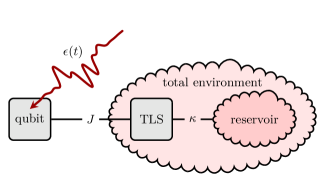
Figure 1: We consider a qubit strongly coupled to a two-level system (TLS) that is weakly coupled to a reservoir. Together, TLS and reservoir define the total environment for the qubit. Due to the strong coupling $J$ between qubit and TLS, the qubit dynamics may become non-Markovian. The TLS-reservoir couples with strength $\kappa$. The coupling between qubit and the reservoir is only indirect.

Our system consists of a qubit in interaction with an external field. The Hamiltonian reads

$$\boldsymbol{\mathsf{\hat{H}}}_{\text{Q}}(t)=-\frac{\hbar\omega_{\text{Q}}}{2}\boldsymbol{\mathsf{\hat{\sigma}}}^{z}_{\text{Q}}-\frac{\hbar\varepsilon(t)}{2}\boldsymbol{\mathsf{\hat{\sigma}}}^{z}_{\text{Q}}.$$ (1)

Here, $\omega_{\text{Q}}$ is the qubit’s level splitting and $\varepsilon(t)$ a control field, to be determined by optimal control theory. $\boldsymbol{\mathsf{\hat{\sigma}}}^{i}$, $i=\{x,y,z\}$, are the usual Pauli matrices.

This single qubit is coupled to an environment that may, in general, give rise to non-Markovian dynamics. Such an environment can be mapped onto a pseudo-mode weakly coupled to a large bath of harmonic modes Garraway and Knight (1996), as depicted in Fig. 1. The pseudo-mode, which acts as a memory, is taken to also be a two-level system (TLS), with Hamiltonian $\boldsymbol{\mathsf{\hat{H}}}_{\text{TLS}}=-\frac{\hbar\omega_{\text{TLS}}}{2}\boldsymbol{\mathsf{\hat{\sigma}}}^{z}_{\text{TLS}}$ and level splitting $\omega_{\text{TLS}}$. The pseudo-mode is not necessarily weakly coupled to the system qubit. We therefore treat the interaction between the system qubit and the memory TLS exactly. This allows to fully capture the correlations we are interested in. For the rest of the environment, we employ the usual approximations, leading to the standard Markovian master equation for the joint state $\boldsymbol{\mathsf{\hat{\rho}}}(t)$ of qubit and TLS Garraway and Knight (1996); Rebentrost et al. (2009); Addis et al. (2014); Reich et al. (2015),

$$\textup{i}\hbar\frac{\text{d}}{\text{d}t}\boldsymbol{\mathsf{\hat{\rho}}}(t) =\left[\boldsymbol{\mathsf{\hat{H}}}(t),\boldsymbol{\mathsf{\hat{\rho}}}(t)\right]+\boldsymbol{\mathsf{\mathcal{L}}}_{D}\left[\boldsymbol{\mathsf{\hat{\rho}}}(t)\right],$$ (2)

$$\boldsymbol{\mathsf{\mathcal{L}}}_{D}\left[\boldsymbol{\mathsf{\hat{\rho}}}(t)\right] =\textup{i}\hbar\sum_{k=1,2}\kappa\left(\boldsymbol{\mathsf{\hat{L}}}_{k}\boldsymbol{\mathsf{\hat{\rho}}}(t)\boldsymbol{\mathsf{\hat{L}}}_{k}^{\dagger}-\frac{1}{2}\left\{\boldsymbol{\mathsf{\hat{L}}}_{k}^{\dagger}\boldsymbol{\mathsf{\hat{L}}}_{k},\boldsymbol{\mathsf{\hat{\rho}}}(t)\right\}\right),$$

with Hamiltonian $\boldsymbol{\mathsf{\hat{H}}}(t)=\boldsymbol{\mathsf{\hat{H}}}_{\text{Q}}(t)\otimes\boldsymbol{\mathsf{\hat{1}}}_{\text{TLS}}+\boldsymbol{\mathsf{\hat{1}}}_{\text{Q}}\otimes\boldsymbol{\mathsf{\hat{H}}}_{\text{TLS}}+\boldsymbol{\mathsf{\hat{H}}}_{\text{int}}$. The interaction between qubit and TLS given by

$$\boldsymbol{\mathsf{\hat{H}}}_{\text{int}} =J\left(\boldsymbol{\mathsf{\hat{\sigma}}}^{x}_{\text{Q}}\otimes\boldsymbol{\mathsf{\hat{\sigma}}}^{x}_{\text{TLS}}\right).$$ (3)

The Lindblad operators $\boldsymbol{\mathsf{\hat{L}}}_{k}$ model the thermal equilibration between the TLS and the remaining reservoir and correspond to those of the optical master equation Breuer and Petruccione (2002), $\boldsymbol{\mathsf{\hat{L}}}_{1}=\sqrt{N+1}(\boldsymbol{\mathsf{\hat{1}}}_{\text{Q}}\otimes\boldsymbol{\mathsf{\hat{\sigma}}}_{\text{TLS}}^{-})$, $\boldsymbol{\mathsf{\hat{L}}}_{2}=\sqrt{N}(\boldsymbol{\mathsf{\hat{1}}}_{\text{Q}}\otimes\boldsymbol{\mathsf{\hat{\sigma}}}_{\text{TLS}}^{+})$, where $N=1/\left(e^{\beta\hbar\omega_{\text{TLS}}}-1\right)$ and $\beta$ is the inverse thermal energy of the reservoir. The state of the qubit is obtained by tracing out the degrees of freedom of the memory TLS at each instant in time, $\boldsymbol{\mathsf{\hat{\rho}}}_{Q}(t)=\textup{Tr}_{\text{TLS}}\left[\boldsymbol{\mathsf{\hat{\rho}}}(t)\right]$.

Cooling requires population relaxation. This motivates our choice of exchange interaction between qubit and memory TLS in Eq. (3). We take the coupling $J$ between qubit and TLS to be larger than the coupling $\kappa$ (otherwise the dynamics of the qubit would be Markovian). On the other hand, $J$ is still small with respect to the level splitting $\omega_{\text{TLS}}$ of the TLS. The corresponding timescale separation ensures detailed balance and accord with the second law of thermodynamics Levy and Kosloff (2014). Note that $\kappa$ refers to a rate, in a physical sense, rather than a coupling strength but, since both can’t be distinguished mathematically, we refer to it as a coupling.

We will analyze several initial states for the qubit and memory TLS. Since the TLS is part of the environment, we always assume it to be initially in thermal equilibrium with the reservoir. To fully understand the role of initial correlations, we start from the factorized case and then generalize it. For the sake of comparability, we assume that the initial state of the qubit is quasi-thermalized with the reservoir as well. Their respective initial states read

$$\boldsymbol{\mathsf{\hat{\rho}}}_{\alpha}^{\text{th}}=\frac{e^{x_{\alpha}}\Ket{0}\Bra{0}+e^{-x_{\alpha}}\Ket{1}\Bra{1}}{2\cosh\left(x_{\alpha}\right)},\qquad x_{\alpha}=\frac{\hbar\omega_{\alpha}\beta}{2},$$ (4)

with $\alpha\in\left\{\text{Q},\text{TLS}\right\}$. In the factorized case, the joint state of qubit and TLS at $t=0$ reads

$$\boldsymbol{\mathsf{\hat{\rho}}}^{\text{init}}_{1}=\boldsymbol{\mathsf{\hat{\rho}}}_{\text{Q}}^{\text{th}}\otimes\boldsymbol{\mathsf{\hat{\rho}}}_{\text{TLS}}^{\text{th}}.$$ (5)

For non-factorizing initial conditions, we first investigate the fully thermalized state of qubit and TLS, which is the steady state and therefore a natural choice. It reads

$$\boldsymbol{\mathsf{\hat{\rho}}}^{\text{init}}_{2}=\boldsymbol{\mathsf{\hat{\rho}}}^{\text{th}}=\frac{1}{Z}\begin{pmatrix}\lambda_{+}&0&0&\zeta_{+}\\ 0&\mu_{+}&\zeta_{-}&0\\ 0&\zeta_{-}&\mu_{-}&0\\ \zeta_{+}&0&0&\lambda_{-}\end{pmatrix},$$ (6)

where $Z=2\left[\cosh\left(x_{+}\right)+\cosh\left(x_{-}\right)\right]$ is the partition function and

$$\delta_{\pm} =\omega_{\text{Q}}\pm\omega_{\text{TLS}},\qquad \lambda_{\pm} =\cosh\left(x_{+}\right)\pm\frac{\delta_{+}}{\Omega_{+}}\sinh\left(x_{+}\right),$$ (7)

$$x_{\pm} =\frac{\Omega_{\pm}\beta}{2},\qquad \mu_{\pm} =\cosh\left(x_{-}\right)\pm\frac{\delta_{-}}{\Omega_{-}}\sinh\left(x_{-}\right),$$

$$\Omega_{\pm} =\sqrt{\delta_{\pm}^{2}+4J^{2}},\qquad \zeta_{\pm} =-\frac{2J}{\Omega_{\pm}}\sinh\left(x_{\pm}\right).$$

Since this state can always be obtained by waiting (or speeding up of thermalisation), the control problem in general is solved, if we can solve it for the steady state. For the chosen parameters Karimi and Pekola (2016), the initial correlations of the thermalized state are rather small. Therefore, to examine the role of initial correlations for the reset in more detail, we artificially add correlations to the factorizing initial state (5),

$$\boldsymbol{\mathsf{\hat{\rho}}}^{\text{init}}_{3}=\boldsymbol{\mathsf{\hat{\rho}}}_{\text{Q}}^{\text{th}}\otimes\boldsymbol{\mathsf{\hat{\rho}}}_{\text{TLS}}^{\text{th}}+\begin{pmatrix}0&0&0&0\\ 0&0&\gamma&0\\ 0&\gamma^{*}&0&0\\ 0&0&0&0\end{pmatrix}.$$ (8)

Motivated by Eq. (6), we chose $\gamma\in\mathbb{R}$ and $\gamma<0$, while ensuring that the result is still a valid density matrix.

We quantify the total amount of correlations in terms of the mutual information $\mathcal{I}$ of qubit and memory TLS Henderson and Vedral (2001). This corresponds to the total amount of correlations, both classical and quantum, between system and environment since the qubit couples directly only to the TLS. To distinguish between classical and quantum correlations, various concepts and measures haven been introduced Modi et al. (2012). Here, we use quantum discord Ollivier and Zurek (2002) to quantify the amount of quantum correlations, which is analytically computable for all considered states Ali et al. (2010). We also calculate entanglement in terms of concurrence Wootters (1998).

If not stated otherwise, $\omega_{\text{TLS}}\neq\omega_{\text{Q}}$ in the following and in particular, $\omega_{\text{TLS}}>\omega_{\text{Q}}$. We set $\hbar=1$ as well as $\omega_{\text{Q}}=1$ which define the units for time and energy, respectively. The chosen parameters are typical for superconducting qubits Devoret and Schoelkopf (2013). In particular, our model could be easily implemented by two superconducting qubits in an RLC circuit Karimi and Pekola (2016), where the resistor acts as a thermal reservoir, or by two superconducting qubits with one of them coupled to a lossy cavity Geerlings et al. (2013).

III Numerical Results

The control problem of qubit reset with the equation of motion (2) and initial conditions (5), (6) and (8) is not easily amenable to an analytical solution. We therefore first determine optimized fields for the reset of the qubit using numerical quantum optimal control Glaser et al. (2015).

III.1 Optimal Control Theory

Assuming that a quantum system can be influenced by external fields $\{\varepsilon_{k}(t)\}$, optimal control theory (OCT) provides the means to maximize or minimize a predefined figure of merit. In our case, the control problem is a simple state-to-state transfer Bartana et al. (1997), achieved within a fixed time $T$. The total optimization functional,

$$F\left[\left\{\varepsilon_{k}\right\}\right]=\epsilon_{T}\left[\boldsymbol{\mathsf{\hat{\rho}}}(T)\right]+\int_{0}^{T}\text{d}t\,g\left[\left\{\varepsilon_{k}(t)\right\},\boldsymbol{\mathsf{\hat{\rho}}}(t),t\right],$$ (9)

consists of the figure of merit $\epsilon_{T}\left[\boldsymbol{\mathsf{\hat{\rho}}}(T)\right]$ and additional constraints, captured in a function $g$. In the following, we consider only a single external field, $\varepsilon(t)$. Our figure of merit is the error in preparing the qubit in the desired target state, irrespective of the TLS state. This can be expressed as Rojan et al. (2014)

$$\epsilon_{T}\left[\boldsymbol{\mathsf{\hat{\rho}}}(T)\right]=1-\left\langle\Psi^{\text{targ}}_{\text{Q}}\right|\textup{Tr}_{\text{TLS}}\left[\boldsymbol{\mathsf{\hat{\rho}}}(T)\right]\left|\Psi^{\text{targ}}_{\text{Q}}\right\rangle\,,$$ (10)

where $\textup{Tr}_{\text{TLS}}\left[\cdot\right]$ describes the partial trace over the TLS. Without loss of generality, we choose the target state $\ket{\Psi^{\text{targ}}_{\text{Q}}}$ to be the bare ground state of the qubit.

We will use Krotov’s method Konnov and Krotov (1999), an iterative optimization algorithm with built-in monotonic convergence Reich et al. (2012), in the following. The constraint function is chosen as

$$g\left[\left\{\varepsilon(t)\right\}\right]=\frac{\lambda}{S(t)}\left(\varepsilon(t)-\varepsilon^{\text{ref}}(t)\right)^{2},$$ (11)

where $\lambda$ is a numerical parameter that controls the update magnitude of the field $\varepsilon(t)$, $S(t)$ a shape function and $\varepsilon^{\text{ref}}(t)$ a reference field (taken to be the field from the previous iteration). The actual update equation from the fields is determined by Eq. (11), the equation of motion (2) and the final time target (10). For more details see Ref. Reich et al. (2012).

III.2 Factorizing Initial State

We start by deriving the optimal reset protocol for a factorizing initial state (5) of qubit and TLS, i.e., when no initial correlation between system and environment, i.e., between qubit and TLS, is present. Note that the level splittings of qubit and TLS are not the same and $\omega_{\text{TLS}}>\omega_{\text{Q}}$. This, together with the identical temperature of qubit and TLS, results in a higher von Neumann entropy of qubit than TLS. According to the second law of thermodynamics, one would expect the best cooling to be achieved by an entropy exchange between TLS and qubit. This has indeed been observed before (Horowitz and Jacobs, 2014; Liuzzo-Scorpo et al., 2016).

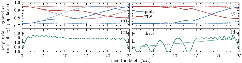
Figure 2: (a,c) Population dynamics induced by the optimized fields (solid lines) for a factorizing initial state, Eq. (5). The corresponding fields are shown in (b,d). The dotted lines illustrate the free evolution of the system, the dashed lines the guess field and its evolution. Left and right hand side used different guess fields for the optimization. Parameters are $\omega_{\text{Q}}=1.0$, $\omega_{\text{TLS}}=3.0$, $J=0.1$, $\kappa=0.04$ and $\beta=1.0$. The initial ground state populations of qubit and TLS are $p_{\text{Q}}^{\text{init}}=0.731$ and $p_{\text{TLS}}^{\text{init}}=0.953$. The final value for the qubit’s population is given by the fidelity $1-\epsilon_{T}=p_{\text{Q}}(T)\approx 0.950$ with error $\epsilon_{T}=5.04\%$ (a,b), respectively $\epsilon_{T}=5.44\%$ (c,d).

For the chosen parameters, entropy exchange can be realized by simply swapping the ground state populations of qubit and TLS. This is best achieved when qubit and TLS are in resonance. As can be seen in Eq. (1), the control field $\varepsilon(t)$ effectively changes the frequency of the qubit. Therefore an educated guess would be to ramp qubit and TLS rapidly into resonance and stay there just long enough for a full swap operation. Figure 2(a) shows the dynamics for this particular guess field (dashed lines), as well as the free evolution (dotted lines) and the dynamics under the optimized field (solid lines). With the optimized field, we indeed obtain the anticipated swap in the ground state populations at $t=T$. In contrast, for the guess field, the maximal $p_{\text{Q}}(t)$ is already achieved at $t\approx 17$.

As we will show analytically in Sec. IV below, the swap is the best and fastest protocol for all factorizing initial conditions when the TLS is initially diagonal in its eigenbasis. The analytical bounds for the minimal error and the shortest possible duration in which the minimal error is reached, given the parameters used in Fig. 2, are

$$\epsilon_{T}^{\text{min}}=1-p_{\text{TLS}}^{\text{th}}=4.74\%,\quad T^{\text{min}}=\frac{\pi}{2J}=15.7.$$ (12)

The actual value of the minimal error $\epsilon_{T}^{\text{min}}$ is determined by the initial ground state population $p_{\text{TLS}}^{\text{th}}$ of the TLS, i.e., it is governed by the reservoir temperature. One might wonder why the minimal time $t\approx 17$ required for the swap in Fig. 2(a) is larger than $T^{\text{min}}$ in Eq. (12). This is due to the fact that, for the sake of experimentally feasible control signals, we do not allow $\varepsilon(t)$ to be instantaneously switched on and off. If we relax this constraint, our optimized control reaches the quantum speed limit $T^{\text{min}}$.

For any time longer than $T^{\text{min}}$, there is always at least one solution achieving maximal cooling but there may be more, i.e., the control strategy is not unique. Another possible control field is shown exemplarily in Fig. 2(d). The non-uniqueness of the solution allows for taking into account further experimentally desirable features, such as restriction of the maximal amplitude of the control, without losing performance.

One may wonder how robust these solutions are to noise in the controls or in the initial state. We have quantified the robustness of the dynamics shown in Fig. 2(a) by averaging over $1000$ realizations of Gaussian amplitude noise for the optimized field shown in Fig. 2(b). For a typical noise level of 1% in the control amplitude, added in form of a varying scaling factor to the control, the final error increases by only a small amount, from 5.04% to 5.16% on average. In order to simulate noise in the initial state, Eq. (5), we have added Gaussian noise to the input parameters $\omega_{\text{Q}}$, $\omega_{\text{TLS}}$ and $\beta$, using again $1000$ realizations. For noise levels up to 2%, we obtain no change in the error at all, and even 10% of state noise increase the error only from 5.04% to 5.18% on average. The protocol is thus very robust with respect to noise in the initial state. The reason for this finding will become clear below in Sec. IV.

III.3 Correlated Initial State

An obvious choice for a correlated initial state is the joint thermal equilibrium state (6) of qubit and TLS. For the chosen parameters, the mutual information of this state is rather small, $\mathcal{I}^{\text{init}}=4.0\cdot 10^{-3}$. The state is separable but has non-zero quantum discord. Note that all initial states studied within this section have non-vanishing quantum discord, since for a thermalized TLS there is no state with only classical correlations.

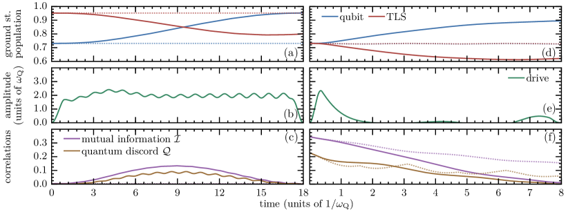
Figure 3: Same as Fig. 2 but with correlated, non-entangled initial states. For the left hand side, the initial state is Eq. (6) and, after optimization, the error at final time becomes $\epsilon_{T}=4.74\%$ and thus coincides with the limit $\epsilon_{T}^{\text{min}}$, cf. Eq. (12). For the right hand side, the initial state is Eq. (8) with $\omega_{\text{Q}}=\omega_{\text{TLS}}=1.0$ and $\gamma=-0.19$. With these level splittings, the error limit for factorizing thermal initial states amounts to $\epsilon_{T}^{\text{min}}=26.9\%$. It is given directly by the initial state since cooling is not possible at all in this case. With initial correlations, the error under the optimized field becomes $\epsilon_{T}=10.52\%$ and is thus much smaller than $\epsilon_{T}^{\text{min}}$ for factorizing initial states.

As can be seen in Fig. 3(a,b,c), both cooling and erasure of correlation is achieved by the optimized control field. The final value of the error in Fig. 3(a), $\epsilon_{T}=4.74\%$, coincides with the minimal error $\epsilon_{T}^{\text{min}}$ for factorizing initial states, cf. Eq. (12). Optimal control therefore allows us to erase initial correlations. A robustness analysis analogous to that for Fig. 2 yields very similar results: Amplitude noise at a level of 1% increases the error from 4.74% to 4.97%, whereas noise in the state has no effect at all up to the 2% level. It increases the error to only 4.85% at the 10% level.

To further investigate the role of initial correlations, we now choose qubit and memory TLS to be in resonance, i.e. $\omega_{\text{Q}}=\omega_{\text{TLS}}$. For factorizing initial conditions, no cooling at all would be possible. Additionally, we enhance the correlations, the initial state is given by Eq. (8). It is thermal in the sense that, if TLS or qubit is traced out, one obtains Eq. (4). Surprisingly, we are not only able to erase the correlations, but even achieve further cooling of the system, as can be seen in Fig. 3(d,e,f), for an initial state with mutual information $\mathcal{I}^{\text{init}}=0.345$ and quantum discord $\mathcal{Q}^{\text{init}}=0.228$. This is clear evidence for system-environment correlations acting as a resource for cooling.

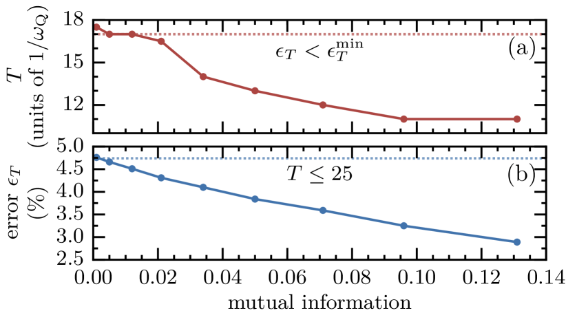
Figure 4: Quantum speed limit (a) and minimal error (b) for a parametrical variation of the strength of initial correlations in Eq. (8). Note that upper and lower panel display results of different optimizations, only their initial states were identical. Panel (a) shows the smallest final time $T$, which still yields an error $\epsilon_{T}<\epsilon_{T}^{\text{min}}$. The dashed line corresponds to the approximate minimal time for a swap operation for factorizing initial states, taking into account finite ramps of the field at the beginning and end, cf. Fig. 2(b). Panel (b) shows the smallest error $\epsilon_{T}$ for any final time satisfying $T\leq 25$. The dashed line corresponds to the limit $\epsilon_{T}^{\text{min}}$ for factorizing initial states, cf. Eq. (12). Same parameters as in Fig. 2.

Remarkably, even the speed limit obtained for factorizing initial conditions does not hold anymore. As can be seen in Fig. 4(a), with increasing total correlations, i.e., mutual information, the error threshold of the factorizing dynamics, $\epsilon_{T}^{\text{min}}$, can be reached in shorter times. Note that although the upper left point in Fig. 4(a) lies above the approximate quantum speed limit for factorizing initial conditions, this is only due to influence of the counter rotating terms (which we will analyze in more detail in Appendix A). If we temporarily neglect the counter rotating terms, the result coincides with the quantum speed limit.

Moreover, Fig. 4(b) shows that the final error $\epsilon_{T}$ is reduced for increasing initial correlations. While we have also studied entangled initial states, the data is not presented here, as the results do not differ. We find that only the amount of mutual information, i.e., the total amount of correlations, not the type, i.e., classical or quantum correlations, is relevant for cooling.

A natural question is whether the speed limit reported in Fig. 4 depends on the type of control over the qubit. It turns out that a control field that couples to the system via $\boldsymbol{\mathsf{\hat{\sigma}}}_{\mathrm{Q}}^{x}$ instead of $\boldsymbol{\mathsf{\hat{\sigma}}}_{\mathrm{Q}}^{z}$ in Eq. (1) does not perform better (data not shown). We have found solutions swapping the populations between qubit and memory TLS also for that type of control when starting from factorizing initial states. Similarly to $\boldsymbol{\mathsf{\hat{\sigma}}}_{\mathrm{Q}}^{z}$-control, correlations in the initial state allow for better reset with smaller errors. However, more time is required in both cases when the control couples via $\boldsymbol{\mathsf{\hat{\sigma}}}_{\mathrm{Q}}^{x}$. As a consequence, the weakly coupled reservoir has a larger impact on the dynamics.

To summarize our findings obtained so far, it is not only possible to reset the qubit in the presence of initial correlations; initial correlations between system and environment can actually be used to enhance the performance of the cooling protocol. Moreover, in the resonant case, initial correlations enable cooling that is impossible without their presence. We analyze the dynamics that lead to this surprising result in more detail in Sec. IV.

III.4 Non-Markovianity

Finally, we investigate whether non-Markovianity of the dynamics has any influence on the optimized fields and achievable final errors. The dynamics of the qubit becomes Markovian or non-Markovian depending on the ratio $J/\kappa$. We quantify this by the accessible volume of state space Lorenzo et al. (2013) to study a possible interplay between non-Markovianity and control.

In our setup, we observe that non-Markovianity seems to be linked to population flow between qubit and memory TLS. More precisely, a monotonic decrease in the qubit’s state space volume can be observed, when populations flows from the memory TLS into the qubit, i.e., increasing the ground state population of the qubit while decreasing it for the memory TLS. This hints towards Markovian dynamics. In contrast, an increase in the state space volume occurs for the reversed population flow, indicating non-Markovian dynamics.

The population flow between qubit and memory TLS is governed by their effective coupling. It is directly influenced by the coupling $J$ and indirectly by the relative detuning $\delta(t)=\omega_{\text{Q}}+\varepsilon(t)-\omega_{\text{TLS}}$ between both. The frequency, with which the population flow changes its direction, increases with $|\delta(t)|$, while its smallest value is assumed for $\delta(t)=0$, where the frequency is entirely determined by $J$. According to this observation, the dynamics of the time-optimal solution (cf. Eq. (12)) turns out to be Markovian. In this case, the ground state population of the qubit is constantly increasing until reaching its maximum at $T^{\text{min}}$. For longer times and non-optimal driving, the controlled dynamics can become non-Markovian, cf. Fig. 2(c,d), as the population flows in both directions at intermediate times. Nevertheless, implementing a swap at $T>T^{\text{min}}$ is also possible with entirely Markovian dynamics, cf. Fig. 2(a,b). This shows that even though non-Markovianity is not crucial for the qubit reset, it also is not harmful in the sense that the optimization does not suppress non-Markovianity.

IV Analytical Results

Two observations in the analysis of the numerical results presented above allow us to simplify our model (2): (i) Solutions obtained under the RWA perform almost equally well in comparison with solutions when the counter-rotating terms are taken into account (we discuss this in more detail in Appendix A). In other words, although the RWA is not a good approximation for the dynamics, it may be invoked to determine the controls. (ii) Two different timescales are relevant to characterize the interaction of the qubit with the environment—a fast one to dump the qubit’s entropy into the pseudo-mode, determined by the coupling $J$, and a slow one leading to re-equilibration, determined by the coupling $\kappa$. Most importantly, the re-equilibration dynamics will never increase the purity of qubit or TLS above their steady state values. The minimum final error and time for the qubit reset are therefore determined only by the fast timescale dynamics.

These observations suggest to neglect the dynamics associated with the slow timescale and described by the Lindblad operators in Eq. (2) as well as the counter-rotating terms in the Hamiltonian (3). As a result, the reset control problem becomes amenable to an analytical solution.

IV.1 Control Equations for Cooling a Qubit

In the following we use concepts from geometric control theory Jurdjevic (1997), where the idea consists in transforming the dynamical equations of the system in such a way that the optimality condition can be expressed analytically Boscain et al. (2002); Sugny et al. (2007). For ease of the derivation, we transform states and Hamiltonian into the rotating frame. Neglecting the counter-rotating terms and the (slow) equilibration with the reservoir, the equation of motion reads

$$\textup{i}\frac{\text{d}}{\text{d}t}\boldsymbol{\mathsf{\hat{\rho}}}^{\prime}(t) =\left[\boldsymbol{\mathsf{\hat{H}}}^{\prime}(t),\boldsymbol{\mathsf{\hat{\rho}}}^{\prime}(t)\right],$$ (13a)

$$\boldsymbol{\mathsf{\hat{H}}}^{\prime}(t) =\begin{pmatrix}\frac{\text{d}\delta(t)}{\text{d}t}\frac{t}{2}&0&0&0\\ 0&\frac{\text{d}\delta(t)}{\text{d}t}\frac{t}{2}&J(t)e^{-\textup{i}\delta(t)t}&0\\ 0&J(t)e^{\textup{i}\delta(t)t}&-\frac{\text{d}\delta(t)}{\text{d}t}\frac{t}{2}&0\\ 0&0&0&-\frac{\text{d}\delta(t)}{\text{d}t}\frac{t}{2}\end{pmatrix},$$ (13b)

where $\delta(t)=\omega_{\text{Q}}+\varepsilon(t)-\omega_{\text{TLS}}$ is the time-dependent detuning of qubit and TLS. For the sake of generality, we account for a possible time-dependence $J=J(t)$ of the coupling strength between qubit and TLS.

For the numerical optimization in section III, the optimization target was to reset the qubit in its ground state. Here, we choose a more general approach and maximize the qubit’s purity . The key idea in the following is to chose a representation of the state $\boldsymbol{\mathsf{\hat{\rho}}}^{\prime}(t)$ in terms of a set of real variables $\left\{x_{1}(t),\dots,x_{16}(t)\right\}$ to span the entire state space of qubit and TLS. Inserting this representation into Eq. (13a), one obtains coupled equations for all $x_{i}$. In order to decouple these equations and reduce the number of relevant variables, one needs to perform an appropriate variable transformation $\left\{x_{1}(t),\dots,x_{16}(t)\right\}\rightarrow\left\{z_{1}(t),\dots,z_{16}(t)\right\}$. A more detailed description of the transformations can be found in Appendix B.

In the new variables, the qubit’s purity becomes

$$\mathcal{P}_{\text{Q}}=\frac{1}{2}+2\left(z_{1}^{2}+z_{5}^{2}+z_{7}^{2}\right)\,,$$ (14)

where we have dropped the explicit time dependence for all quantities. The corresponding equations of motion are decoupled into two separate subspaces. On the one hand, we have

$$\begin{pmatrix}\dot{z}_{1}\\ \dot{z}_{2}\\ \dot{z}_{3}\end{pmatrix}=2J_{1}\begin{pmatrix}-z_{2}\\ z_{1}-z_{1}^{\text{c}}\\ 0\end{pmatrix}+2J_{2}\begin{pmatrix}-z_{3}\\ 0\\ z_{1}-z_{1}^{\text{c}}\end{pmatrix}+2\alpha\begin{pmatrix}0\\ -z_{3}\\ z_{2}\end{pmatrix},$$ (15)

describing the dynamics of the qubit’s ground state population, $p_{\text{Q}}=z_{1}+1/2$, within the three-dimensional subspace $S_{1}=\left\{z_{1},z_{2},z_{3}\right\}$, $z_{1}^{\text{c}}$ being a constant. Note that $z_{2}$, $z_{3}$ are non-zero at time $t=0$ only if initial correlations are present, cf. Eqs. (8), (36) and (39). Equation (15) thus already indicates that initial correlations can be transferred into ground state population and hence purity. On the other hand, the qubit’s coherences, $\gamma_{\text{Q}}=z_{5}+\textup{i}z_{7}$, evolve within the four-dimensional subspace $S_{2}=\left\{z_{5},z_{6},z_{7},z_{8}\right\}$,

$$\begin{pmatrix}\dot{z}_{5}\\ \dot{z}_{6}\\ \dot{z}_{7}\\ \dot{z}_{8}\end{pmatrix}=J_{1}\begin{pmatrix}-z_{6}\\ z_{5}\\ z_{8}\\ -z_{7}\end{pmatrix}+J_{2}\begin{pmatrix}z_{8}\\ -z_{7}\\ z_{6}\\ -z_{5}\end{pmatrix}+2\alpha\begin{pmatrix}z_{7}\\ 0\\ -z_{5}\\ 0\end{pmatrix},$$ (16)

where $z_{6}$ and $z_{8}$ are related to the TLS coherence. The three fields are given by

$$J_{1}=J\cos(\delta t),\quad J_{2}=J\sin(\delta t),\quad\alpha=\frac{1}{2}\frac{\text{d}\delta}{\text{d}t}t.$$ (17)

It is straightforward to show that the dynamics within the subspaces $S_{1}$ and $S_{2}$ is restricted to the surface of two spheres. For $S_{1}$, we find from Eq. (15)

$$\frac{\text{d}}{\text{d}t}R_{1}^{2}=0,\qquad R_{1}=\sqrt{\left(z_{1}-z_{1}^{\text{c}}\right)^{2}+z_{2}^{2}+z_{3}^{2}},$$ (18)

with $R_{1}$ the radius of the sphere centered around $\left(z_{1}^{\text{c}},0,0\right)$ with constant $z_{1}^{\text{c}}=-(z_{4}+1)/2$, cf. Eq. (39). Similarly for $S_{2}$, Eq. (16) yields

$$\frac{\text{d}}{\text{d}t}R_{2}^{2}=0,\qquad R_{2}=\sqrt{z_{5}^{2}+z_{6}^{2}+z_{7}^{2}+z_{8}^{2}},$$ (19)

with radius $R_{2}$ and center $\left(0,0,0,0\right)$. The values of $R_{1}$ and $R_{2}$ are determined by the initial values $z_{i}^{\text{init}}$ with $i=1,\dots,8$. In other words, the accessible part of the entire state space is fully determined by the initial state $\boldsymbol{\mathsf{\hat{\rho}}}^{\text{init}}=\boldsymbol{\mathsf{\hat{\rho}}}(0)=\boldsymbol{\mathsf{\hat{\rho}}}^{\prime}(0)$.

IV.2 Optimal Strategy for Thermal Factorizing Initial States

The factorizing initial state (5) is obviously diagonal. Thus we have $z_{2}^{\text{init}}=z_{3}^{\text{init}}=0$ as well as $z_{i}^{\text{init}}=0$, $i=5,\dots,8$. As a consequence, $R_{2}=0$, i.e., no dynamics will occur in $S_{2}$, and the relevant subspace is entirely given by $S_{1}$. In the following, we parametrize Eq. (5) as

$$\boldsymbol{\mathsf{\hat{\rho}}}^{\text{init}}=\boldsymbol{\mathsf{\hat{\rho}}}_{\text{Q}}^{\text{th}}\otimes\boldsymbol{\mathsf{\hat{\rho}}}_{\text{TLS}}^{\text{th}}=\begin{pmatrix}a_{\text{Q}}&0\\ 0&b_{\text{Q}}\end{pmatrix}\otimes\begin{pmatrix}a_{\text{TLS}}&0\\ 0&b_{\text{TLS}}\end{pmatrix},$$ (20)

and assume $\boldsymbol{\mathsf{\hat{\rho}}}_{\text{TLS}}^{\text{th}}$ to be initially more pure than $\boldsymbol{\mathsf{\hat{\rho}}}_{\text{Q}}^{\text{th}}$. This amounts to $a_{\text{TLS}}^{2}+b_{\text{TLS}}^{2}>a_{\text{Q}}^{2}+b_{\text{Q}}^{2}$ with $a,b$ the ground and excited state populations of qubit and TLS, respectively. We first discuss the resonant case, i.e., $\delta=0$ for all $t$, and derive the time-optimal solution for the control problem. Second, we show that allowing for $\delta\neq 0$ does not improve the best possible final purity of the qubit.

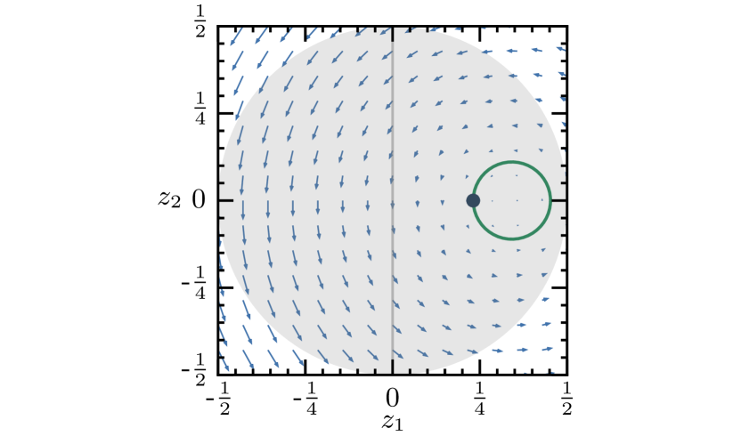
Figure 5: Evolution of the qubit ground state population $p_{\text{Q}}=z_{1}+1/2$ (green line) within the subspace $S_{1}^{2}$ for non-vanishing coupling strength $J\neq 0$ and factorizing initial state (5), indicated by the large dot (parameters as in Fig. 2). Qubit and TLS are in resonance ($\delta=0$ for all $t$) and the evolution of the state along the green line is determined by the vector field (21) (blue arrows). The gray vertical line indicates the minimal purity (respectively, ground state population) of the qubit, cf. Eq. (14) with $z_{5}=z_{7}=0$. The gray sphere in the background visualizes the projection of the entire state space onto the two-dimensional subspace $\left\{z_{1},z_{2}\right\}$.

For $\delta=0$ for all $t$, which implies $J_{1}=J$ and $J_{2}=\alpha=0$, Eq. (15) is further simplified and the dynamics are confined to the two-dimensional subspace $S_{1}^{2}=\left\{z_{1},z_{2}\right\}$,

$$\begin{pmatrix}\dot{z}_{1}\\ \dot{z}_{2}\end{pmatrix}=2J\begin{pmatrix}-z_{2}\\ z_{1}-z_{1}^{\text{c}}\end{pmatrix}.$$ (21)

Figure 5 shows the accessible state space for the dynamics within $S_{1}^{2}$ when starting in the initial state used in Fig. 2. Depending on the sign of $J$, the initial state evolves along the vector field ($J>0$) or opposite to it ($J<0$), cf. Eq. (21). The optimization target can then be trivially identified as the point with maximal $z_{1}$ on this curve. Assuming constant positive coupling $J$, the state will evolve with constant speed along the green line in Fig. 5. It then takes $T^{\text{min}}=\pi/(2J)$ to reach the rightmost point. This can simply be shown by integrating along the green line. Allowing for time-dependent coupling $J(t)\geq 0$, the minimal time is given by

$$\int_{0}^{T^{\text{min}}}J(t)\text{d}t=\frac{\pi}{2}.$$ (22)

Therefore, the time-optimal solution is to choose $J(t)$ maximal for all $t$.

The point of maximum qubit purity, $\mathcal{P}_{\text{Q}}^{\text{max}}$, is determined by the center $z_{1}^{\text{c}}$ of the sphere and its radius $R_{1}$,

$$\mathcal{P}_{\text{Q}}^{\text{max}}=\frac{1}{2}+2\left(z_{1}^{\text{c}}+R_{1}\right)^{2}=a_{\text{TLS}}^{2}+b_{\text{TLS}}^{2}=\mathcal{P}_{\text{TLS}}^{\text{init}},$$ (23)

with $\mathcal{P}_{\text{TLS}}^{\text{init}}$ the initial TLS purity. Equations (22) and (23) hold for any initial factorizing state of the form (20) with the TLS initially purer than the qubit. Note that for $z_{1}^{\text{c}}<0$, Eq. (23) becomes $\mathcal{P}_{\text{Q}}^{\text{max}}=\frac{1}{2}+2\left(z_{1}^{\text{c}}-R_{1}\right)^{2}$ but yields identical results.

It is straightforward to see that a non-vanishing time-dependent detuning $\delta\neq 0$ does not provide access to states with higher qubit purity. The dynamics is confined to the surface of the three-dimensional sphere $S_{1}$, cf. Eq. (18), and the point of maximal purity is already accessible with $\delta=0$ for all $t$. It is important to note that $\delta\neq 0$ involves dynamics in the $z_{3}$-dimension. This becomes crucial when starting with initially correlated states.

IV.3 Optimal Strategy for Factorizing Initial States with Coherences

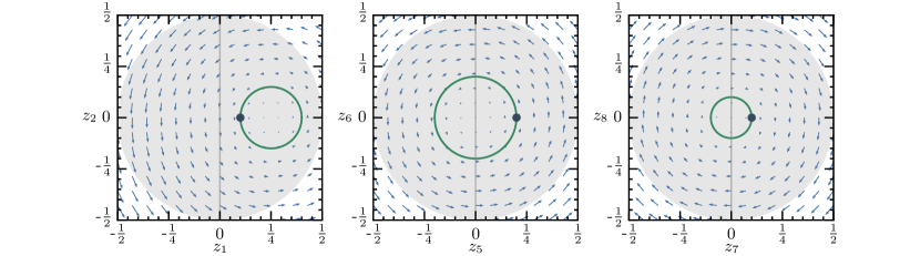
Figure 6: Time evolution (green lines) within the three subspaces $S_{1}^{2}$, $S_{2}^{2}$ and $S_{3}^{2}$ (from left to right) for a factorizing initial state (24) with $a_{\text{Q}}=0.6$, $b_{\text{Q}}=0.4$, $\gamma_{\text{Q}}=0.2+\textup{i}0.1$ and $a_{\text{TLS}}=0.9$, $b_{\text{TLS}}=0.1$, $\gamma_{\text{TLS}}=0$. Qubit and TLS are in resonance ($\delta=0$ for all $t$). The dots indicate the initial state within the specific subspace, which then evolves along the vector fields (21) and (25), represented by the blue arrows. The gray vertical lines indicate the respective minimal contribution to the qubit’s purity for each subspace, while the gray spheres visualize the projection of the entire state space onto the subspaces.

The most general initially factorizing state for qubit and TLS is given by

$$\boldsymbol{\mathsf{\hat{\rho}}}^{\text{init}}=\boldsymbol{\mathsf{\hat{\rho}}}_{\text{Q}}\otimes\boldsymbol{\mathsf{\hat{\rho}}}_{\text{TLS}}=\begin{pmatrix}a_{\text{Q}}&\gamma_{\text{Q}}\\ \gamma_{\text{Q}}^{*}&b_{\text{Q}}\end{pmatrix}\otimes\begin{pmatrix}a_{\text{TLS}}&\gamma_{\text{TLS}}\\ \gamma_{\text{TLS}}^{*}&b_{\text{TLS}}\end{pmatrix},$$ (24)

with $a,b$ as in Eq. (20) and $\gamma_{\text{Q}},\gamma_{\text{TLS}}$ the coherences of qubit and TLS. We first consider the case $\gamma_{\text{TLS}}=0$. From a physical perspective, this is a well justified initial state, since we assume the TLS to be in permanent contact with the reservoir and thus in thermal equilibrium. In contrast, for the qubit, non-zero coherences, $\gamma_{\text{Q}}\neq 0$, are a possible scenario, e.g., as a result of its previous use in a computation. In this case, we again find $z_{2}^{\text{init}}=z_{3}^{\text{init}}=0$. However, $z_{5}=\mathfrak{Re}\left\{\gamma_{\text{Q}}\right\}$ or $z_{7}=\mathfrak{Im}\left\{\gamma_{\text{Q}}\right\}$ or both will be non-zero. Note that $z_{6}^{\text{init}}=z_{8}^{\text{init}}=0$ still holds but there is dynamics within the subspace $S_{2}$, since $R_{2}\neq 0$.

Assuming resonance in the following (i.e., $\delta=0$ for all $t$), the dynamics within $S_{1}$ is reduced to the two-dimensional subspace $S_{1}^{2}$, as discussed before. Similarly, the dynamics in the four-dimensional subspace $S_{2}$ decouple and can be described by two two-dimensional subspaces, $S_{2}^{2}$ and $S_{3}^{2}$. Their respective equations of motions are

$$\begin{pmatrix}\dot{z}_{5}\\ \dot{z}_{6}\end{pmatrix}=J\begin{pmatrix}-z_{6}\\ z_{5}\end{pmatrix},\qquad\begin{pmatrix}\dot{z}_{7}\\ \dot{z}_{8}\end{pmatrix}=J\begin{pmatrix}z_{8}\\ -z_{7}\end{pmatrix}.$$ (25)

Figure 6 shows the evolution in the three subspaces $S_{1}^{2}$, $S_{2}^{2}$ and $S_{3}^{2}$ for an exemplary initial factorizing state with $\gamma_{\text{Q}}\neq 0$ and $\gamma_{\text{TLS}}=0$. We now have dynamics in all three subspaces. As before, maximizing the qubit’s ground state population, $p_{\text{Q}}=z_{1}+1/2$, requires the time $T=\pi/(2J)$, which corresponds to evolution in terms of a half circle in $S_{1}^{2}$. Importantly, the motion within $S_{1}^{2}$ is twice as fast as that in $S_{2}^{2}$ and $S_{3}^{2}$, which can be easily seen by comparing Eqs. (21) and (25). Therefore, at time $T=\pi/(2J)$, the qubit’s coherences, $\gamma_{\text{Q}}=z_{5}+\textup{i}z_{7}$, vanish, since the evolution within $S_{2}^{2}$ and $S_{3}^{2}$ only runs through a quarter circle. The minimal reset time is thus not changed when allowing for coherences in the initial qubit state. This finding is in line with the observation that for pure states (as considered in this section), standard quantum speed limit bounds coincide with the bound obtained from the Wigner-Yanase skew information which particularly quantifies the coherence of a state (relative to the eigenbasis of the Hamiltonian)  Marvian et al. (2016); Pires et al. (2016). Moreover, as long as the initial purities of qubit and TLS satisfy $\mathcal{P}_{\text{Q}}^{\text{init}}<\mathcal{P}_{\text{TLS}}^{\text{init}}$, the time-optimal solution is still the swap operation given by Eqs. (22) and (23). This is true irrespective of the specific initial state of the qubit.

If we allow for coherences also in the initial state of the TLS, $\gamma_{\text{TLS}}\neq 0$, this does not hold anymore. In this case, some or all of the initial values $z_{2}^{\text{init}}$, $z_{3}^{\text{init}}$, $z_{6}^{\text{init}}$ and $z_{8}^{\text{init}}$ are non-zero. Geometrically, the large dots in the three spheres $S_{1}^{2}$, $S_{2}^{2}$ and $S_{3}^{2}$ in Fig. 6 are then placed at arbitrary points along the green curves. Thus, the evolution cannot easily be synchronized in terms of half and quarter circles. Rather, exact knowledge of the initial state would be required to determine the optimal solution.

IV.4 Optimal Strategy for Correlated Initial States

For correlated initial states, the dynamics involving the qubit ground state population $z_{1}$ explores all three dimensions of the subspace $S_{1}$ spanned by $z_{1},z_{2},z_{3}$. We show that a geometric analysis is still useful in this case since it provides physical insight into the control mechanisms of the optimal solution. In particular, it explains why initial correlations result in a higher purity and a shorter time for the reset.

For any initial state satisfying Eq. (8), no dynamics occurs in $S_{2}^{2}$ and $S_{3}^{2}$. It is then straightforward to show that these correlated initial states allow to access states with higher purity than factorizing states: Since the reduced states of qubit and TLS are unchanged by the presence of correlations, the center $\left(z_{1}^{\text{c}},0,0\right)$ of the sphere in $S_{1}$ remains the same, while its radius $R_{1}$ increases, cf. Eq. (18). As a result, the set of accessible states that may be reached by the dynamics is enlarged.

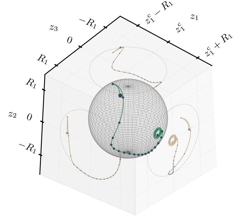
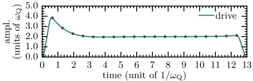
Figure 7: Evolution within the subspace $S_{1}$ (top panel) for a correlated initial state of the form (8) under the optimized field shown in the bottom panel ($\gamma=-0.09$, all other parameters as in Fig. 2). The large dot marks the initial point in state space, the small dots indicate the evolution in chunks of $5\%$ of the total time. The final error is $\epsilon_{T}=1.6\%$, achieved within $T=13$.

Figure 7 shows the evolution starting from a correlated initial state under a field designed by numerical optimization. It illustrates why the quantum speed limit for factorizing initial states can be beaten. For the initial state in Fig. 7, $z_{2}^{\text{init}}=0$ and $z_{3}^{\text{init}}<0$. The optimized field drives the state rapidly towards the $z_{3}=0$ plane. This is achieved by the characteristic off-resonant peak in the optimized field between $t=0$ and $t=2$. The subsequent evolution with $\delta=0$ becomes two-dimensional within the $z_{1}$-$z_{2}$ plane; it is equivalent to that in Fig. 5 discussed above. However, in contrast to the dynamics shown in Fig. 5, the motion in the $z_{1}$-$z_{2}$ plane has to overcome a reduced distance as a consequence of the initial transfer between $z_{3}<0$ and $z_{3}=0$. It can be seen from the projection of the entire motion onto the $z_{1}$-$z_{2}$ plane (shown in the front left plane in Fig. 7 top, note in particular the position of the third small dot), that less than a half circle has to be overcome by the evolution with $\delta=0$ to reach the point of largest purity, $z_{1,\text{max}}=z_{1}^{\text{c}}+R_{1}$. Since the initial transfer towards the $z_{3}=0$ plane is accomplished faster than any motion within this plane, the total time is reduced. Unfortunately, however, the reduction in time comes at a cost, namely the control field must be tuned to the initial value of $z_{3}$. In other words, for correlated initial states, derivation of the optimal control strategy requires knowledge of the initial state.

This analysis can be completed by a geometric description of the solution. To this end, we consider the differential system (15) and assume the coupling $J$ to be bounded, while there is no constraint on $\frac{\text{d}\delta}{\text{d}t}$, i.e., on $\alpha(t)$, cf. Eq. (17). As in the numerical optimization, the optimal solution can be decomposed into two steps. In a first stage, we neglect the first two terms on the right hand side of Eq. (15) and the $\alpha$-term is used to move arbitrarily fast in the $z_{2}$-$z_{3}$ plane from the initial point into the $z_{3}=0$ plane. This motion is completed in a short time $\tau_{\varepsilon}$ provided $\alpha(t)$ satisfies the condition

$$\int_{0}^{\tau_{\varepsilon}}2\alpha(t)\text{d}t=\frac{\pi}{2},$$ (26)

which, after integration by parts, leads to

$$\delta(\tau_{\varepsilon})-\int_{0}^{\tau_{\varepsilon}}\delta(t)\text{d}t=\frac{\pi}{2}.$$ (27)

A standard solution for $\delta$ is given by a linear time evolution of the form

$$\delta(t)=\frac{\pi t}{2\tau_{\varepsilon}(1-\tau_{\varepsilon}/2)}\quad\mathrm{for}\quad t\in[0,\tau_{\varepsilon}].$$ (28)

The second part of the optimal solution is the meridian trajectory in the $z_{3}=0$ plane with $\delta(t)=0$. In fact, for $\delta(t)$ constant, we recover the Grushin model Sugny and Kontz (2008). It can be shown (using the appendix of Ref. Sugny and Kontz (2008)) that the meridian trajectory is the solution minimizing the time to reach the state of largest purity, $z_{1,\textrm{max}}$. The time required for the motion along the meridian is fixed by the initial point of this dynamics, it is $T^{\textrm{min}}=\theta^{\text{init}}/(2J)$ where $\theta^{\text{init}}$ is the polar angle of the sphere $S_{1}$ given by $z_{1}^{\text{init}}=R_{1}\cos(\theta^{\text{init}})$. Assuming the time to reach the $z_{3}=0$ plane, $\tau_{\varepsilon}$, to be arbitrarily small, the time $\tau_{\varepsilon}+T^{\textrm{min}}$ required for both steps of the time-optimal solution for correlated initial states is smaller than the time of $\pi/(2J)$ obtained with factorizing initial states. This rigorously confirms the role of initial correlations for the speedup of the purification process.

The robustness of the numerical control solutions with respect to noise in either control amplitude or initial state, observed in Sec. III, can be rationalized by the analytical solutions found here. Key to all of the reset strategies is a population swap between qubit and TLS. This is independent of the actual populations, as evidenced in the remarkable robustness with respect to noise in the initial state. The population swap requires resonance between qubit and TLS. Amplitude noise up to a level of 1% does not perturb the resonance sufficiently to have a noticeable effect on the final errors.

V Summary and Conclusions

We have shown that quantum optimal control theory allows to derive protocols for qubit reset with minimal error in minimum time. Such fast and reliable qubit reset is crucial for quantum devices to be used multiple times or quantum machines to operate in a cyclic way. Our main assumption was that the qubit is coupled to a structured environment, consisting of a pseudo-mode and a reservoir. Note that introducing more than one pseudo-mode will not change the overall picture since the reset will be determined by the most strongly coupled mode, in analogy with Ref. Reich et al. (2015). The coupling to the pseudo-mode is taken to be small compared to the level spacings but large enough to render the qubit dynamics non-Markovian; the coupling to the reservoir is weak. We have assumed the system-pseudomode coupling to be of $\boldsymbol{\mathsf{\hat{\sigma}}}_{x}\boldsymbol{\mathsf{\hat{\sigma}}}_{x}$-type. This is motivated by the fact that cooling requires population exchange. In an actual experiment, the pseudo-mode could be realized by an ancilla, and the reservoir by a resistor or a lossy cavity—scenarios that are found for example in superconducting circuits.

The assumptions of our model imply two timescales—a fast one for the interaction between qubit and TLS (pseudo-mode) and a slow one for re-equilibration with the reservoir. This timescale separation allows to solve the reset control problem analytically and evaluate the bounds for minimum error and minimum time for certain initial states and under the rotating wave approximation. Assuming the TLS to be initially in thermal equilibrium with the reservoir, we find different solutions to the control problem for factorizing and correlated initial states. If qubit and TLS are initially uncorrelated (and thus there are no correlations between qubit and all of the environment), the time-optimal solution is a swap operation. Cooling and reset are thus only possible if the TLS is initially colder, i.e., purer, than the qubit. The minimal error is determined by the temperature as well as the initial difference in the qubit and TLS level splittings, it becomes smaller for larger TLS splitting. The minimal time is set by the coupling strength between qubit and TLS. The time-optimal solution consists in ramping qubit and TLS into and out off resonance. Since this is most easily achieved by an external control field coupling to the system via $\boldsymbol{\mathsf{\hat{\sigma}}}_{z}$, $\boldsymbol{\mathsf{\hat{\sigma}}}_{z}$-controls outperform controls coupling to the system via $\boldsymbol{\mathsf{\hat{\sigma}}}_{x}$. The time-optimal solution is valid for all factorizing initial states of qubit and TLS (with the TLS initially in thermal equilibrium with the reservoir), i.e., no a priori knowledge of the initial qubit state is necessary. If initial correlations between qubit and environment are present, the limits on minimum error and minimum time for the uncorrelated case both can be beaten. However, in this case, knowledge of the initial state is required to derive the reset protocol since the control strategy is tied to the amount of initial correlations. This information is easily accessible, if the initial state is e.g. the steady state of a non-weakly coupled system.

The control technique that we have employed here is open loop which is the method of choice when one seeks time-optimal solutions Glaser et al. (2015). There also exist a number of closed-loop feedback control approaches to qubit purification. They are based on continuous measurement and use feedback to control the qubit in such a way that the qubit’s purification rate increases Combes and Jacobs (2006); Wiseman and Ralph (2006); Wiseman and Bouten (2008); Combes et al. (2010). While the requirement of carrying out measurements is the price to pay with closed-loop approaches, they come with the advantage of inherent robustness to noise. In contrast, open-loop control per se is not robust to noise, although it can be made so Rojan et al. (2014); Goerz et al. (2014). We have therefore assessed the robustness of our control solutions by adding Gaussian-distributed noise to both the amplitude of the control and to the initial state. Our solutions are robust to amplitude noise up to about 1%. When realizing our model consisting of a qubit and a pseudo-mode with two superconducting qubits, such a noise level by far exceeds typical experimental values Quintana et al. (2017). Moreover, we have found noise in the initial state to not affect the final reset error all the way up to a level of 10%. This remarkable robustness is explained by the time-optimal control strategy consisting in a population swap between qubit and pseudo-mode.

Both speed-up and error reduction in the presence of initial correlations can be understood by the geometry of the evolution in state space. Remarkably, even in the case where qubit and TLS are initially in resonance and cooling would not be possible at all for factorizing initial conditions, correlations allow for entropy export. Initial correlations with the environment thus act as a resource for the qubit reset. Quantifying the initial correlations in terms of the mutual information, quantum discord and entanglement of qubit and TLS, we have found the amounts by which error and time can be reduced to be directly linked to the mutual information. In contrast, the type of correlation turns out not to play any role. In other words, entanglement between system and environment is not required and classical, or at least quantum correlation without entanglement, are sufficient to beat the limits on error and time for factorizing initial states.

Our findings suggest to actively exploit initial correlations between qubit and environment in qubit reset, using either a single ancilla qubit or true defect. For example for superconducting qubits, the latter can be characterized precisely both in terms of level splitting and coupling Shalibo et al. (2010) and thus effectively act like an ancilla Reich et al. (2015). For optimum performance of the qubit reset, the amount of initial correlations must be known. The idea is then to engineer the initial correlations between the qubit and its environment before carrying out the reset. This is related to algorithmic cooling where correlations are created dynamically by cross-relaxation Rodriguez-Briones et al. (2017a) or measurements of interacting qubits Rodriguez-Briones et al. (2017b). However, our approach differs in two important ways—it operates at the quantum speed limit and assumes controllability only for the system, not the bath.

Even when correlations are not created on purpose, they emerge inevitably when components are coupled. This is ignored in theoretical proposals that assume factorizing initial conditions. Executing time-optimal qubit reset with and without artificially engineered initial correlations would allow for an experimental comparison between factorizing and non-factorizing initial conditions. This would be an important step towards a better understanding of open quantum systems.

Enhancement of initial correlations by use of an ancialla or defect provides a fresh perspective onto quantum reservoir engineering Poyatos et al. (1996). So far, protocols for quantum reservoir engineering have targeted the creation of non-trivial quantum states as steady state of some driven-dissipative dynamics, see e.g. Poyatos et al. (1996); Pielawa et al. (2007); Diehl et al. (2008); Kastoryano et al. (2011), assuming the evolution to be Markovian and the coupling to the environment to be weak. While we have found non-Markovianity per se not to be relevant for the success of qubit reset, we show that strong coupling to an engineered environment allows for faster protocols and the emerging correlations to be useful for a further speed up of the evolution. This suggests to explore quantum reservoir engineering in scenarios beyond the weak coupling and Markov approximations.

Appendix A Influence of the Counter Rotating Terms

For obtaining analytical results, we need to employ the rotating wave approximation (RWA). In the following, we therefore examine the influence of the counter rotating terms in the interaction Hamiltonian (3). It can be rewritten,

$$\boldsymbol{\mathsf{\hat{H}}}_{\text{int}} =J\left(\boldsymbol{\mathsf{\hat{\sigma}}}^{+}_{\text{Q}}\otimes\boldsymbol{\mathsf{\hat{\sigma}}}^{+}_{\text{TLS}}+\boldsymbol{\mathsf{\hat{\sigma}}}^{+}_{\text{Q}}\otimes\boldsymbol{\mathsf{\hat{\sigma}}}^{-}_{\text{TLS}}\right.$$ (29)

$$\qquad\left.+\boldsymbol{\mathsf{\hat{\sigma}}}^{-}_{\text{Q}}\otimes\boldsymbol{\mathsf{\hat{\sigma}}}^{+}_{\text{TLS}}+\boldsymbol{\mathsf{\hat{\sigma}}}^{-}_{\text{Q}}\otimes\boldsymbol{\mathsf{\hat{\sigma}}}^{-}_{\text{TLS}}\right),$$

where $\boldsymbol{\mathsf{\hat{\sigma}}}^{-}$ ($\boldsymbol{\mathsf{\hat{\sigma}}}^{+}$) are the usual lowering (raising) operators for two-level systems. The counter rotating terms are given by $\boldsymbol{\mathsf{\hat{\sigma}}}_{\text{Q}}^{+}\otimes\boldsymbol{\mathsf{\hat{\sigma}}}_{\text{TLS}}^{+}$ and $\boldsymbol{\mathsf{\hat{\sigma}}}_{\text{Q}}^{-}\otimes\boldsymbol{\mathsf{\hat{\sigma}}}_{\text{TLS}}^{-}$; they are often neglected as part of a RWA. As we will show, these terms contribute to the dynamics, i.e., the RWA is not a good approximation here. Nevertheless, they have only a minor influence on the solution of the reset control problem.

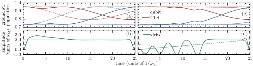
Figure 8: Identical to Fig. 2 but employing the RWA (30) for dynamics and optimizations. For the final errors, we find $\epsilon_{T}=5.01\%$ (a,b) and $\epsilon_{T}=5.41\%$ (c,d).

In the RWA, the interaction Hamiltonian becomes

$$\boldsymbol{\mathsf{\hat{H}}}_{\text{int}}^{\text{RWA}} =J\left(\boldsymbol{\mathsf{\hat{\sigma}}}^{+}_{\text{Q}}\otimes\boldsymbol{\mathsf{\hat{\sigma}}}^{-}_{\text{TLS}}+\boldsymbol{\mathsf{\hat{\sigma}}}^{-}_{\text{Q}}\otimes\boldsymbol{\mathsf{\hat{\sigma}}}^{+}_{\text{TLS}}\right).$$ (30)

Repeating the optimizations for the factorizing initial state (5) under the RWA yields errors that are slightly smaller ($\epsilon_{T}=5.01\%$ in Fig. 8(a,b) and $\epsilon_{T}=5.41\%$ in Fig. 8(c,d)), compared to the case when the counter-rotating terms are included ($\epsilon_{T}=5.04\%$ in Fig. 2(a,b) and $\epsilon_{T}=5.44\%$ in Fig. 2(c,d)). Employing the optimized fields from Fig. 8 in the dynamics including the counter rotating terms (without further optimization) results in only slightly increased final errors $\epsilon_{T}=5.12\%$ (a,b) and $\epsilon_{T}=5.49\%$ (c,d). The errors are thus affected only in the third digit, despite the dynamics and optimized fields in Figs. 2 and 8 being visibly different.

In order to repeat this analysis for non-factorizing initial states, we have to adjust the joint thermal state (6) of qubit and TLS,

$$\boldsymbol{\mathsf{\hat{\rho}}}^{\text{init}}_{2,\text{RWA}}=\boldsymbol{\mathsf{\hat{\rho}}}^{\text{th}}_{\text{RWA}}=\frac{1}{Z}\begin{pmatrix}e^{\phi}&0&0&0\\ 0&\lambda+\frac{\delta}{\Omega}\mu&-\frac{2J}{\Omega}\mu&0\\ 0&-\frac{2J}{\Omega}\mu&\lambda-\frac{\delta}{\Omega}\mu&0\\ 0&0&0&e^{-\phi}\end{pmatrix},$$ (31)

where $\lambda=\cosh(x)$, $\mu=\sinh(x)$ and partition function $Z=2\cosh\left(\phi\right)+2\cosh\left(x\right)$ with

$$\delta =\omega_{\text{Q}}-\omega_{\text{TLS}},\qquad \phi =\frac{\left(\omega_{\text{Q}}+\omega_{\text{TLS}}\right)\beta}{2},$$ (32)

$$x =\frac{\Omega\beta}{2},\qquad \Omega =\sqrt{\delta^{2}+4J^{2}}.$$

The optimized final error in the RWA becomes $\epsilon_{T}=4.73\%$, compared to $\epsilon_{T}=4.74\%$ in Fig. 3(a,b,c). Using the RWA-optimized field in the dynamics including the counter-rotating terms increases the final error to only $\epsilon_{T}=4.78\%$. This is particularly remarkable, since not only the interaction Hamiltonians differ, but also the initial states, cf. Eqs. (6) and (31). Similarly, for very strong initial correlations, we find $\epsilon_{T}=10.4\%$, compared to $\epsilon_{T}=10.5\%$ in Fig. 3(d,e,f); and use of the RWA-optimized field in dynamics with the counter rotating terms increases the error to only $\epsilon_{T}=10.6\%$. Similarly, we find our analysis of the quantum speed limit and minimal achievable error in Fig. 4 to be essentially independent of the RWA.

The small increase of the errors when using the RWA-optimized fields in dynamics that include the counter-rotating terms is explained by larger final residual correlations. However, the increase due to the counter-rotating terms is of the order of $10^{-4}$, whereas all final errors quoted above correspond to residual correlations of the order of $10^{-3}$. Overall, the increase is thus negligible, and we conclude that the counter-rotating terms, while modifying the dynamics, have no relevant influence on the achievable final error or, in other words, the controllability of the problem. This has two important implications: First, in order to identify control solutions for the reset problem, it is sufficient to consider the interaction Hamiltonian in the RWA (30). This will allow an analytical treatment, see Sec. IV below. Moreover, from an experimental perspective, a loss of fidelity in the third digit is irrelevant and it might actually be advantageous to use RWA-optimized fields, since these are generally much smoother, cf. Fig. 2(b,d) and Fig. 8(b,d).

Appendix B Variable transformations

The RWA-Hamiltonian, neglecting counter rotating terms, reads

$$\boldsymbol{\mathsf{\hat{H}}}^{\text{RWA}}(t) =\boldsymbol{\mathsf{\hat{H}}}_{\text{Q}}(t)\otimes\boldsymbol{\mathsf{\hat{1}}}_{\text{TLS}}+\boldsymbol{\mathsf{\hat{1}}}_{\text{Q}}\otimes\boldsymbol{\mathsf{\hat{H}}}_{\text{TLS}}+\boldsymbol{\mathsf{\hat{H}}}^{\text{RWA}}_{\text{int}}$$ (33)

$$=\boldsymbol{\mathsf{\hat{H}}}_{0}(t)+\boldsymbol{\mathsf{\hat{H}}}^{\text{RWA}}_{\text{int}},$$

with $\boldsymbol{\mathsf{\hat{H}}}^{\text{RWA}}_{\text{int}}$ defined as in Eq. (30). Performing a unitary transformation with transformation operator

$$\boldsymbol{\mathsf{\hat{O}}}(t)=\text{exp}\left\{-\textup{i}\boldsymbol{\mathsf{\hat{H}}}_{0}^{\text{RWA}}(t)t\right\}$$ (34)

yields a transformed state $\boldsymbol{\mathsf{\hat{\rho}}}^{\prime}(t)$ and Hamiltonian $\boldsymbol{\mathsf{\hat{H}}}^{\prime}(t)$,

$$\boldsymbol{\mathsf{\hat{\rho}}}^{\prime}(t) =\boldsymbol{\mathsf{\hat{O}}}^{\dagger}(t)\boldsymbol{\mathsf{\hat{\rho}}}(t)\boldsymbol{\mathsf{\hat{O}}}(t),$$ (35)

$$\boldsymbol{\mathsf{\hat{H}}}^{\prime}(t) =\boldsymbol{\mathsf{\hat{O}}}^{\dagger}(t)\boldsymbol{\mathsf{\hat{H}}}(t)\boldsymbol{\mathsf{\hat{O}}}(t)-\textup{i}\boldsymbol{\mathsf{\hat{O}}}^{\dagger}(t)\frac{\text{d}\boldsymbol{\mathsf{\hat{O}}}(t)}{\text{d}t}.$$

This yields the Liouville-von Neumann equation (13a). Starting from there, we summarize in the following the variable transformations required to derive Eqs. (15) and (16) in Section IV.1. First, we represent the density matrix in the rotating frame, $\boldsymbol{\mathsf{\hat{\rho}}}^{\prime}(t)$, in terms of $16$ real variables, $x_{i}(t)\in\mathbb{R}$, dropping the explicit time-dependence for all quantities in the following,

$$\boldsymbol{\mathsf{\hat{\rho}}}^{\prime}=\begin{pmatrix}x_{1}&x_{5}+\textup{i}x_{6}&x_{7}+\textup{i}x_{8}&x_{9}+\textup{i}x_{10}\\ x_{5}-\textup{i}x_{6}&x_{2}&x_{11}+\textup{i}x_{12}&x_{13}+\textup{i}x_{14}\\ x_{7}-\textup{i}x_{8}&x_{11}-\textup{i}x_{12}&x_{3}&x_{15}+\textup{i}x_{16}\\ x_{9}-\textup{i}x_{10}&x_{13}-\textup{i}x_{14}&x_{15}-\textup{i}x_{16}&x_{4}\end{pmatrix}\,.$$ (36)

The set $\left\{x_{1},\dots,x_{16}\right\}$ spans the entire state space, and the equation of motion (13a) becomes

$$\dot{\vec{x}}=J_{1}\vec{f}_{1}(\vec{x})+J_{2}\vec{f}_{2}(\vec{x})+\alpha\vec{f}_{3}(\vec{x}),$$ (37a)

with $$\vec{x}=\left(x_{1},\dots,x_{16}\right)^{\top}$$,

$$\vec{f}_{1}=\begin{pmatrix}0\\ -2x_{12}\\ 2x_{12}\\ 0\\ -x_{8}\\ x_{7}\\ -x_{6}\\ x_{5}\\ 0\\ 0\\ 0\\ x_{2}-x_{3}\\ x_{16}\\ -x_{15}\\ x_{14}\\ -x_{13}\end{pmatrix},\quad\vec{f}_{2}=\begin{pmatrix}0\\ -2x_{11}\\ 2x_{11}\\ 0\\ -x_{7}\\ -x_{8}\\ x_{5}\\ x_{6}\\ 0\\ 0\\ x_{2}-x_{3}\\ 0\\ -x_{15}\\ -x_{16}\\ x_{13}\\ x_{14}\end{pmatrix},\quad\vec{f}_{3}=\begin{pmatrix}0\\ 0\\ 0\\ 0\\ 0\\ 0\\ 2x_{8}\\ -2x_{7}\\ 2x_{10}\\ -2x_{9}\\ 2x_{12}\\ -2x_{11}\\ 2x_{14}\\ -2x_{13}\\ 0\\ 0\end{pmatrix}.$$ (37b)

and $J_{1}$, $J_{2}$ and $\alpha$ given in Eq. (17). The vector fields $\vec{f}_{1}(\vec{x})$ $\vec{f}_{2}(\vec{x})$ and $\vec{f}_{3}(\vec{x})$ govern the admissible directions for the evolution of the state $\vec{x}$, whereas $J_{1}$, $J_{2}$ and $\alpha$ determine their relative magnitude for each direction. With the representation (36), the purity of the qubit becomes

$$\mathcal{P}_{\text{Q}} =\left(x_{1}+x_{2}\right)^{2}+\left(x_{3}+x_{4}\right)^{2}$$ (38)

$$\quad+2\left(x_{7}+x_{13}\right)^{2}+2\left(x_{8}+x_{14}\right)^{2}.$$

The set of the coupled equations (37) is separated in two disjunct sets by introducing new variables, $z_{i}\in\mathbb{R}$. The relevant ones are given by

$$z_{1} =x_{1}+x_{2}-1/2,\qquad z_{5}=x_{7}+x_{13},$$ (39)

$$z_{2} =x_{12},\qquad z_{6}=x_{6}-x_{16},$$

$$z_{3} =x_{11},\qquad z_{7}=x_{8}+x_{14},$$

$$z_{4} =-2x_{1}-x_{2}-x_{3},\qquad z_{8}=x_{5}-x_{15}.$$

There are eight further variables, $z_{9},\dots,z_{16}$, that are required to span the entire state space. However, these variables are not coupled to $z_{1},\dots,z_{8}$, so they can be ignored for the maximization of the purity.

Using the new variables and exploiting that $\textup{Tr}\left[\boldsymbol{\mathsf{\hat{\rho}}}^{\prime}\right]=x_{1}+x_{2}+x_{3}+x_{4}=1$, the qubit purity simplifies to Eq. (14). Moreover, the equations of motion for $z_{1},\dots,z_{8}$ decouple into two independent subspaces. One subspace is $S_{1}=\left\{z_{1},z_{2},z_{3}\right\}$ with the equations of motion given in Eq. (15), where $z_{1}^{\text{c}}=-\left(z_{4}+1\right)/2$ is a constant since $\dot{z}_{4}=0$. The other subspace is $S_{2}=\left\{z_{5},z_{6},z_{7},z_{8}\right\}$ with the equations of motion given by Eq. (16).

References

- DiVincenzo (2000) D. P. DiVincenzo, Fortschr. Phys. 48, 771 (2000).
- Fernandez et al. (2004) J. Fernandez, S. Lloyd, T. Mor, and V. Roychowdhury, Int. J. Quantum Inform. 2, 461 (2004).
- Ladd et al. (2010) T. D. Ladd, F. Jelezko, R. Laflamme, Y. Nakamura, C. Monroe, and J. O’Brien, Nature 464, 45 (2010).
- Reed et al. (2010) M. D. Reed, B. R. Johnson, A. A. Houck, L. DiCarlo, J. M. Chow, D. I. Schuster, L. Frunzio, and R. J. Schoelkopf, Appl. Phys. Lett. 96, 203110 (2010).
- Ristè et al. (2012) D. Ristè, J. G. van Leeuwen, H.-S. Ku, K. W. Lehnert, and L. DiCarlo, Phys. Rev. Lett. 109, 050507 (2012).
- Johnson et al. (2012) J. E. Johnson, C. Macklin, D. H. Slichter, R. Vijay, E. B. Weingarten, J. Clarke, and I. Siddiqi, Phys. Rev. Lett. 109, 050506 (2012).
- Govia and Wilhelm (2015) L. C. G. Govia and F. K. Wilhelm, Phys. Rev. Applied 4, 054001 (2015).
- Kosloff and Levy (2014) R. Kosloff and A. Levy, Annu. Rev. Phys. Chem. 65, 365 (2014).
- Gelbwaser-Klimovsky et al. (2015) D. Gelbwaser-Klimovsky, W. Niedenzu, and G. Kurizki, Adv. At. Mol. Opt. Phys. 64, 329 (2015).
- Roßnagel et al. (2016) J. Roßnagel, S. T. Dawkins, K. N. Tolazzi, O. Abah, E. Lutz, F. Schmidt-Kaler, and K. Singer, Science 352, 325 (2016).
- Karimi and Pekola (2016) B. Karimi and J. P. Pekola, Phys. Rev. B 94, 184503 (2016).
- Watanabe et al. (2017) G. Watanabe, B. P. Venkatesh, P. Talkner, and A. del Campo, Phys. Rev. Lett. 118, 050601 (2017).
- Geerlings et al. (2013) K. Geerlings, Z. Leghtas, I. M. Pop, S. Shankar, L. Frunzio, R. J. Schoelkopf, M. Mirrahimi, and M. H. Devoret, Phys. Rev. Lett. 110, 120501 (2013).
- Horowitz and Jacobs (2014) J. M. Horowitz and K. Jacobs, Phys. Rev. E 89, 042134 (2014).
- Liuzzo-Scorpo et al. (2016) P. Liuzzo-Scorpo, L. A. Luis A. Correa, R. Schmidt, and G. Adesso, Entropy 18, 48 (2016).
- Tuorila et al. (2016) J. Tuorila, M. Partanen, T. Ala-Nissila, and M. Möttönen, arXiv:1612.04160 (2016).
- Weiss (2012) U. Weiss, Quantum Dissipative Systems, 4th ed. (World Scientific, 2012).
- Glaser et al. (2015) S. J. Glaser, U. Boscain, T. Calarco, C. P. Koch, W. Köckenberger, R. Kosloff, I. Kuprov, B. Luy, S. Schirmer, T. Schulte-Herbrüggen, D. Sugny, and F. K. Wilhelm, Eur. Phys. J. D 69, 279 (2015).
- Schmidt et al. (2011) R. Schmidt, A. Negretti, J. Ankerhold, T. Calarco, and J. T. Stockburger, Phys. Rev. Lett. 107, 130404 (2011).
- Rebentrost et al. (2009) P. Rebentrost, I. Serban, T. Schulte-Herbrüggen, and F. K. Wilhelm, Phys. Rev. Lett. 102, 090401 (2009).
- Reich et al. (2015) D. M. Reich, N. Katz, and C. P. Koch, Sci. Rep. 5, 12430 (2015).
- Garraway and Knight (1996) B. M. Garraway and P. L. Knight, Phys. Rev. A 54, 3592 (1996).
- Addis et al. (2014) C. Addis, B. Bylicka, D. Chruściński, and S. Maniscalco, Phys. Rev. A 90, 052103 (2014).
- Breuer and Petruccione (2002) H.-P. Breuer and F. Petruccione, The theory of open quantum systems, 1st ed. (Oxford University Press, 2002).
- Levy and Kosloff (2014) A. Levy and R. Kosloff, EPL (Europhysics Letters) 107, 20004 (2014).
- Henderson and Vedral (2001) L. Henderson and V. Vedral, J. Phys. A 34, 6899 (2001).
- Modi et al. (2012) K. Modi, A. Brodutch, H. Cable, T. Paterek, and V. Vedral, Rev. Mod. Phys. 84, 1655 (2012).
- Ollivier and Zurek (2002) H. Ollivier and W. Zurek, Phys. Rev. Lett. 88, 01790 (2002).
- Ali et al. (2010) M. Ali, A. R. P. Rau, and G. Alber, Phys. Rev. A 81, 042105 (2010).
- Wootters (1998) W. K. Wootters, Phys. Rev. Lett. 80, 2245 (1998).
- Devoret and Schoelkopf (2013) M. H. Devoret and R. J. Schoelkopf, Science 339, 1169 (2013).
- Bartana et al. (1997) A. Bartana, R. Kosloff, and D. J. Tannor, J. Chem. Phys. 106, 1435 (1997).
- Rojan et al. (2014) K. Rojan, D. M. Reich, I. Dotsenko, J.-M. Raimond, C. P. Koch, and G. Morigi, Phys. Rev. A 90, 023824 (2014).
- Konnov and Krotov (1999) A. I. Konnov and V. F. Krotov, Autom. Rem. Contr. 60, 1427 (1999).
- Reich et al. (2012) D. M. Reich, M. Ndong, and C. P. Koch, J. Chem. Phys. 136, 104103 (2012).
- Lorenzo et al. (2013) S. Lorenzo, F. Plastina, and M. Paternostro, Phys. Rev. A 88, 020102 (2013).
- Jurdjevic (1997) V. Jurdjevic, Geometric Control Theory, 1st ed. (Cambridge University Press, 1997).
- Boscain et al. (2002) U. Boscain, G. Charlot, J.-P. Gauthier, S. Guérin, and H.-R. Jauslin, J. Math. Phys. 43, 2107 (2002).
- Sugny et al. (2007) D. Sugny, C. Kontz, and H. R. Jauslin, Phys. Rev. A 76, 023419 (2007).
- Note (1) This is also possible in the numerical optimization. However, the more complicated target functional requires a significantly more sophisticated optimization algorithm Reich et al. (2012).
- Note (2) For mixed states, these bounds do not coincide, and the Wigner-Yanase skew information provides a tighter bound, highlighting the role of coherences for the speed of evolution Marvian et al. (2016); Pires et al. (2016).
- Marvian et al. (2016) I. Marvian, R. W. Spekkens, and P. Zanardi, Phys. Rev. A 93, 052331 (2016).
- Pires et al. (2016) D. P. Pires, M. Cianciaruso, L. C. Céleri, G. Adesso, and D. O. Soares-Pinto, Phys. Rev. X 6, 021031 (2016).
- Sugny and Kontz (2008) D. Sugny and C. Kontz, Phys. Rev. A 77, 063420 (2008).
- Combes and Jacobs (2006) J. Combes and K. Jacobs, Phys. Rev. Lett. 96, 010504 (2006).
- Wiseman and Ralph (2006) H. M. Wiseman and J. F. Ralph, New J. Phys. 8, 90 (2006).
- Wiseman and Bouten (2008) H. M. Wiseman and L. Bouten, Quant. Inf. Proc. 7, 71 (2008).
- Combes et al. (2010) J. Combes, H. M. Wiseman, K. Jacobs, and A. J. O’Connor, Phys. Rev. A 82, 022307 (2010).
- Goerz et al. (2014) M. H. Goerz, E. J. Halperin, J. M. Aytac, C. P. Koch, and K. B. Whaley, Phys. Rev. A 90, 032329 (2014).
- Quintana et al. (2017) C. M. Quintana, Y. Chen, D. Sank, A. G. Petukhov, T. C. White, D. Kafri, B. Chiaro, A. Megrant, R. Barends, B. Campbell, Z. Chen, A. Dunsworth, A. G. Fowler, R. Graff, E. Jeffrey, J. Kelly, E. Lucero, J. Y. Mutus, M. Neeley, C. Neill, P. J. J. O’Malley, P. Roushan, A. Shabani, V. N. Smelyanskiy, A. Vainsencher, J. Wenner, H. Neven, and J. M. Martinis, Phys. Rev. Lett. 118, 057702 (2017).
- Shalibo et al. (2010) Y. Shalibo, Y. Rofe, D. Shwa, F. Zeides, M. Neeley, J. M. Martinis, and N. Katz, Phys. Rev. Lett. 105, 177001 (2010).
- Rodriguez-Briones et al. (2017a) N. A. Rodriguez-Briones, J. Li, X. Peng, T. Mor, Y. Weinstein, and R. Laflamme, arXiv:1703.02999 (2017a).
- Rodriguez-Briones et al. (2017b) N. A. Rodriguez-Briones, E. Martin-Martinez, A. Kempf, and R. Laflamme, arXiv:1703.03816 (2017b).
- Poyatos et al. (1996) J. F. Poyatos, J. I. Cirac, and P. Zoller, Phys. Rev. Lett. 77, 4728 (1996).
- Pielawa et al. (2007) S. Pielawa, G. Morigi, D. Vitali, and L. Davidovich, Phys. Rev. Lett. 98, 240401 (2007).
- Diehl et al. (2008) S. Diehl, A. Micheli, A. Kantian, B. Kraus, H.-P. Büchler, and P. Zoller, Nature Phys. 4, 878 (2008).
- Kastoryano et al. (2011) M. J. Kastoryano, F. Reiter, and A. S. Sørensen, Phys. Rev. Lett. 106, 090502 (2011).