Partition function of free conformal fields
in 3-plet representation

Abstract

Simplest examples of AdS/CFT duality correspond to free CFTs in $d$ dimensions with fields in vector or adjoint representation of an internal symmetry group dual in the large $N$ limit to a theory of massless or massless plus massive higher spins in AdS_d+1. One may also study generalizations when conformal fields belong to higher dimensional representations, i.e. carry more than two internal symmetry indices. Here we consider the case of the 3-fundamental ("3-plet") representation. One motivation is a conjectured connection to multiple M5-brane theory: heuristic arguments suggest that it may be related to an (interacting) CFT of 6d (2,0) tensor multiplets in 3-plet representation of large $N$ symmetry group that has an AdS₇ dual. We compute the singlet partition function $Z$ on $S^{1}\times S^{d-1}$ for a free field in 3-plet representation of $U(N)$ and analyse its novel large $N$ behaviour. The large $N$ limit of the low temperature expansion of $Z$ which is convergent in the vector and adjoint cases here is only asymptotic, reflecting the much faster growth of the number of singlet operators with dimension, indicating a phase transition at very low temperature. Indeed, while the critical temperatures in the vector ($T_{c}\sim N^{\gamma},\ \gamma>0)$ and adjoint ($T_{c}\sim 1$) cases are finite, we find that in the 3-plet case $T_{c}\sim(\log N)^{-1}$, i.e. it approaches zero at large $N$. We discuss some details of large $N$ solution for the eigenvalue distribution. Similar conclusions apply to higher $p$-plet representations of $U(N)$ or $O(N)$ and also to the free $p$-tensor theories invariant under $[U(N)]^{p}$ or $[O(N)]^{p}$ with $p\geq 3$.

Imperial-TP-AT-2017-04

1 Introduction

Examples of unitary conformal field theories are free theories containing scalar, spinor or $({{d\over 2}-1})$-form fields in $d$ dimensions. Assuming that these fields transform in some representation of a global $U(N)$ or $O(N)$ symmetry group one expects that in the large $N$ limit this theory should be dual to a theory in AdS_d+1. The latter should contain a tower of massless higher spins dual to bilinear conserved currents as well as an infinite collection of massive higher spins dual to primary operators containing irreducible ("single-trace") contractions of more than two fields.

The simplest case is that of a fundamental (vectorial) representation Klebanov:2002ja ; Giombi:2016ejx ; Giombi:2016pvg where the spectrum is particularly simple, containing conserved currents in $CFT_{d}$ or massless higher spins in AdS_d+1. The dual AdS theory is then a massless higher spin theory with $N$ as the coefficient in front of the classical action.

Another well-known example is when the free fields (e.g. spin-1 vectors in 4d) belong to the adjoint representation Sundborg:2000wp ; HaggiMani:2000ru ; Bae:2016rgm ; Bae:2016hfy ; Bae:2017spv . Here the dual AdS theory should be string-like: in addition to massless higher spin fields it should contain also families of massive fields which together may have an interpretation of a spectrum of a "tensionless" string theory in AdS_d+1. The coupling constant on the AdS side is then $1/N$, i.e. the coefficient in front of the AdS field theory action is $N^{2}$.

Here we would like to study the next in complexity case when the CFT field belongs to a 3-fundamental or "3-plet" representation, i.e. to a general, symmetric or antisymmetric 3-index tensor representation of a global symmetry group. Already in the simplest case of the scalar field the spectrum of "single-trace" operators with more than two fields (dual to massive fields in AdS) here is much more intricate than in the adjoint case, suggestive of a "tensionless membrane" interpretation. The coefficient in front of the dual AdS field theory action should now be $N^{3}$.

The spectrum of CFT operators on $\mathbb{R}^{d}$ (or states in $\mathbb{R}\times S^{d-1}$) is naturally encoded in the small temperature $T=\beta^{-1}$ or small $x=e^{-\beta}$ expansion of the partition function $Z(x)$ on $S^{1}_{\beta}\times S^{d-1}$. The singlet-state large $N$ partition function was previously computed in the $U(N)$ Shenker:2011zf and the $O(N)$ Jevicki:2014mfa ; Giombi:2014yra vector representation case and was matched to the corresponding massless higher spin partition function in AdS. The partition function in the adjoint representation case was computed in Sundborg:1999ue ; Polyakov:2001af ; Aharony:2003sx (see also Skagerstam:1983gv ; Schnitzer:2004qt ; Barabanschikov:2005ri ) and its matching to the AdS partition function was discussed in Bae:2016rgm ; Bae:2016hfy ; Bae:2017spv . Once the temperature becomes large enough (of order $N^{\gamma}$ with $\gamma>0$ in the vector case and $\gamma=0$ in the adjoint case) these partition functions exhibit phase transitions Shenker:2011zf ; Sundborg:1999ue ; Aharony:2003sx that may have some dual AdS interpretation (cf. Amado:2016pgy ).

Here we will compute the singlet partition function $Z(x)$ in the case of a free CFT in a 3-plet (i.e. 3-index tensor) representation of internal symmetry group. We shall analyse its small temperature expansion matching the direct operator count and also present the large $N$ solution of the corresponding matrix model implying the presence of a phase transition at small $x_{c}=e^{-\beta_{c}}$ of order of $N^{-a}$ with $a>0$, i.e. at $T_{c}={a\over\log N}$.

1.1 Heuristic motivation: 3-plet (2,0) tensor multiplet as M5-brane theory

Before turning to the details of analysis of the large $N$ limit of the 3-plet partition function let us first make some speculative remarks providing a motivation behind this work which is related to attempts to understand a 6d CFT describing $N\gg 1$ coinciding M5-branes Witten:1995zh ; Strominger:1995ac ; kt1 ; kt2 ; Gubser:1997yh ; Seiberg:1997ax ; Gubser:1998nz ; Henningson:1998gx ; Harvey:1998bx ; Aharony:1999ti ; Bastianelli:1999ab ; Bastianelli:2000hi ; Tseytlin:2000sf ; t1 ; Beccaria:2014qea ; Beccaria:2015ypa .

The idea that $N^{3}$ scaling of observables in the multiple M5-brane case may be explained in terms of M2-branes with three holes attached to three different M5-branes thus leading to 3-index world volume fields was originally suggested in kt2 . Then a natural proposal that a 6d superconformal theory describing multiple M5-branes should involve $(2,0)$ tensor multiplets in 3-tensor representation of $SU(N)$ or $SO(N)$ was made in Bastianelli:1999ab ; t1 .

To recall, the structure of a world-volume theory of a single M5-brane follows from consideration of symmetries and collective coordinates corresponding to the classical M5-brane solution in 11d supergravity Gueven:1992hh ; Callan:1991ky ; Gibbons:1993sv ; Kaplan:1995cp . It is represented by a free $(2,0)$ tensor multiplet containing (anti)selfdual 3-form $H_{\mu\nu\lambda}=3\partial_{[\mu}B_{\nu\lambda]}$, 5 scalars $\phi_{r}$ and 2 Weyl fermions $\psi_{a}$. This is an example of a free 6d CFT with conformal anomalies and correlators that can be directly computed Bastianelli:1999ab ; Bastianelli:2000hi .

In the case of multiple D-branes the low energy theory is the SYM theory, i.e. one gets $N^{2}$ vector multiplets at weak coupling and that matches the leading $N^{2}$ scaling predicted by the dual supergravity for BPS observables. By formal analogy, one needs $N^{3}$ free tensor multiplets to match the leading large $N$ scaling of protected 11d supergravity observables kt1 ; kt2 ; Harvey:1998bx ; Bastianelli:1999ab ; Bastianelli:2000hi . This suggests that the $(2,0)$ multiplet should carry a 3-index representation of an internal symmetry group that has dimension $\propto N^{3}$ at large $N$. Thus, if the conjectured 6d theory were to have a weak coupling limit its field content would be $(B^{ijk}_{\mu\nu},\phi^{ijk}_{r},\psi^{ijk}_{a})$ with $i,j,k=1,2,...,N$.

The reason why the M5-brane world-volume 2-form field may carry 3 internal indices can be heuristically argued for as follows kt2 ; Bastianelli:1999ab ; kt1 . Replacing the standard picture of multiple D-branes connected by open strings by M5-branes connected by M2-branes one may attempt to explain the $N^{3}$ scaling of multiple M5-brane entropy kt1 by assuming that triple M5-brane connections by "pants-like" membrane surfaces are providing the dominant contribution (pair-wise "cylinder" connections should give subleading $N^{2}$ contributions).

Alternatively, one may think of an interacting (2,0) tensor multiplet theory as a low-energy limit of a tensionless 6d string theory with closed strings carrying internal 3-plet indices which originate from virtual membranes connecting three parallel M5-branes: when the M5-branes get close, the membranes with 3 holes may effectively reduce to strings that then have 3 internal labels and thus $B^{ijk}_{\mu\nu}$ massless modes. The correlation between the 3 Lorentz indices and the 3 internal indices of the corresponding field strength $H^{ijk}_{\mu\nu\lambda}=dB^{ijk}_{\mu\nu}$ is thus a direct analog of the fact that the YM field strength which is a rank 2 Lorentz tensor carries also 2 internal indices (takes values in adjoint representation).

Ignoring the self-duality constraint on $H_{\mu\nu\lambda}$ one may start with a free theory

$$L_{0}=H^{ijk}_{\mu\nu\lambda}H^{ijk}_{\mu\nu\lambda}\ ,\ \ \ \ \ \ \ \ \ \ \ \ \ \delta B^{ijk}_{\mu\nu}=\partial_{[\mu}\epsilon^{ijk}_{\nu]}\ ,$$ (1)

where $\epsilon^{ijk}_{\mu}$ is a gauge parameter. A speculative idea of how to generalize this to an interacting theory is to assume that the role of the would-be structure constants here should be played by the generalized field strength $\widehat{H}^{ijk}_{\mu\nu\lambda}$ itself, i.e. that a non-linear generalization of the transformation rule for $B$ in (1) should have the following structure

$$\widehat{\delta}B^{ijk}_{\mu\nu}=\partial_{[\mu}\epsilon^{ijk}_{\nu]}+\widehat{H}^{ij^{\prime}k^{\prime}}_{\mu\rho\lambda}B^{i^{\prime}jk^{\prime}}_{\nu\rho}\epsilon^{i^{\prime}j^{\prime}k}_{\lambda}+...\ ,\qquad\qquad\widehat{H}^{ijk}_{\mu\nu\lambda}=\partial_{[\mu}B^{ijk}_{\nu\lambda]}+\widehat{H}^{ij^{\prime}k^{\prime}}_{\mu\rho\kappa}B^{i^{\prime}jk^{\prime}}_{\nu\rho}B^{i^{\prime}j^{\prime}k}_{\lambda\kappa}+...\ ,$$ (2)

where dots stand for terms with other possible contractions of indices. The full non-linear field strength $\widehat{H}$ should then be non-polynomial in $B$. Such couplings required to contract 3-plet internal indices may have a generalization to self-dual case and may correspond to a "soft" gauge algebra structure (thus possibly avoiding no-go arguments against the existence of an interacting chiral antisymmetric tensor theory in Bekaert:1999dp ; Bekaert:1999ue ).

One consequence of this 3-index assumption is that the leading interaction between the $B^{ijk}_{\mu\nu}$-fields should be quartic t1 rather than cubic as in the adjoint-representation YM theory

$$L=\widehat{H}^{ijk}_{\mu\nu\lambda}\widehat{H}^{ijk}_{\mu\nu\lambda}\ \ \to\ \ \partial B^{ijk}\partial B^{ijk}+B^{ijk}B^{ij^{\prime}k^{\prime}}\partial B^{i^{\prime}jk}\partial B^{i^{\prime}j^{\prime}k}+....={\rm G}(B)\partial B\partial B+...\ .$$ (3)

Adding scalar fields of tensor multiplets one may expect to get similar non-linear interactions, e.g., through covariant derivative $\ D_{\mu}\phi^{ijk}=\partial_{\mu}\phi^{ijk}+\widehat{H}^{ij^{\prime}k^{\prime}}_{\mu\rho\kappa}B^{i^{\prime}jk^{\prime}}_{\rho\kappa}\phi^{i^{\prime}j^{\prime}k}+...$. Supersymmetry may require also quartic and higher self-interactions of the 3-plet scalars and fermions.

Even assuming such a hypothetical interacting $(2,0)$ tensor multiplet theory may exist at the classical level, one faces several difficult questions. The canonical dimension of the free $B$-field in $6d$ is 2 and thus $H$ has dimension 3. Then the classical interactions in (2),(3) require a dimensional coupling parameter and thus break the classical conformal invariance of the free theory (1). One is then to hope that at the quantum level there may exist a non-trivial conformal fixed point at which the dimension of $B$ becomes 0. Another important question is about an existence of a well-defined large $N$ limit in such theory. The multiple M5-brane theory should certainly admit a large $N$ expansion, as suggested, e.g., by the presence of 11d M-theory corrections to its anomalies Harvey:1998bx ; Tseytlin:2000sf ; Beccaria:2014qea ; Beccaria:2015ypa (see also Beem:2014kka ; Cordova:2015vwa ) and its free energy Gubser:1998nz which are subleading in $N$ compared to the leading $N^{3}$ term.

As a starting point, one may consider just a free 3-plet tensor multiplet CFT which correctly describes the $N^{3}$ term in the anomalies and protected 3-point functions as predicted by the 11d supergravity. Regardless of its precise connection to multiple M5-brane theory, it should have a consistent AdS₇ dual on its own right. Our aim below will be to study the thermal partition function in such free tensor multiplet theory with fields in a 3-index representation of an internal symmetry group.

1.2 Structure of the paper

Below we shall mostly concentrate on the $S^{1}\times S^{d-1}$ partition function a free scalar field in a 3-fundamental representation of $U(N)$. The cases of symmetric or antisymmetric 3-plet representation, $O(N)$ symmetry and 3-tensors with distinguishable indices will be similar. The generalization to free fermions or $({{d\over 2}-1})$-form fields and thus, in particular, to a (2,0) tensor multiplet will be straightforward.

As we shall review in section 2, this partition function encodes the spectrum of "single-trace" primary operators in the free CFT. The singlet constraint may be implemented as in the familiar vector or adjoint representation cases by coupling the 3-plet field to a flat $U(N)$ connection and integrating over its non-trivial holonomy on $S^{1}$, i.e. over a constant matrix $U\in U(N)$. For a free field $\Phi$ in a general real representation $R$ of $U(N)$ the resulting expression for the partition function $Z(x)$,  $x=e^{-\beta}$ will be given by the matrix $U$ integral in (10) with the "action" in the exponential depending on the character $\chi_{R}(U)$ and the one-particle partition function $z_{\Phi}(x)$.

In section 3 we shall compute the low temperature (small $x$) expansion of $Z$ in the large $N$ limit. We shall first expand the integral (10) in powers of $x$ at finite $N$ and then take $N\to\infty$. While in the familiar cases of the vector and adjoint representations the low temperature, $N=\infty$ expansions are convergent (and thus the $x\to 0$ and $N\to\infty$ limits commute in the low temperature phase $T\leq T_{c}$), in the 3-plet case this expansion will be only asymptotic. The reason for this will be a rapid growth of the number of singlet operators with their dimension which will lead to the vanishing of the radius of convergence $x_{c}$ or the critical temperature $T_{c}$ in the $N=\infty$ limit. We shall find a closed expression (46) for the $N=\infty$ limit of the small $x$ expansion of $Z$ that encodes the number of singlet operators built out of elementary 3-plet fields to any order in dimension.

The analysis of the phase structure of $Z(x)$ at large but finite $N$ will be carried out in 4. We shall rewrite the integral representation for $Z$ in terms of the eigenvalue density and study the large $N$ stationary-point solution for it. We shall find that in the 3-plet case there is a phase transition at the critical temperature $T_{c}\sim\frac{1}{\log\,N}$ which approaches zero at $N\to\infty$. At finite $N$ there are always two phases, $0<T\leq T_{c}$ and $T>T_{c}$, while at $N=\infty$ the first phase becomes essentially the $T=0$ one, so there is only the second phase for any $T>0$. As in the vector and adjoint cases, we will find that in the $T>T_{c}$ phase the large $N$ stationary point solution for the eigenvalue density leads to $\log Z=\mathcal{O}(N^{2})$.

Some concluding remarks about open issues will be made in section 5. Few technical details and extensions will be presented in Appendices. In particular, the case of 2-plet representation will be discussed in Appendix A. The $O(N)$ case will be considered in Appendix D. In Appendix C.2 we shall compute the value of the eigenvalue density action on the stationary-point solution in the 3-plet case. In Appendix E we shall give a general relation for the "single-trace" partition function counting only irreducible contractions in terms of the full $Z$.

In Appendix C.4 we shall analyze the singlet partition function of a $p$-tensor with all indices being different, i.e. transforming under a separate copy of $U(N)$ as in the tensor models in Witten:2016iux ; Klebanov:2016xxf . It turns out that the case of such $[U(N)]^{p}$ theory is very similar to the $U(N)$ one discussed above, with $p=3$ being again the critical value when the small temperature expansion becomes only asymptotic in the large $N$ limit, i.e. with the critical temperature being again $T_{c}(N\to\infty)\to 0.$

2 Partition function with singlet constraint

Given a CFT, one may be interested (in particular, in the context of AdS/CFT duality) in its thermal partition function $Z$ with a singlet constraint (see, e.g., Skagerstam:1983gv ; Sundborg:1999ue ; Aharony:2003sx ; Schnitzer:2004qt ; Schnitzer:2006xz ; Shenker:2011zf ). We shall consider a free field $\Phi$ in $S^{1}_{\beta}\times S^{d-1}$ transforming in a representation of the global symmetry group. The singlet projection may be implemented by coupling $\Phi$ to a flat connection $A_{\mu}=U^{-1}\partial_{\mu}U$ and integrating over it. Only the constant part of the $A_{0}$ component cannot be gauged away because of the non-trivial holonomy along the thermal circle. The resulting partition function $Z$ is then given by the 1-loop determinant with $A_{0}$-dependent covariant derivatives integrated over the constant eigenvalues of $A_{0}$ Aharony:2003sx ; Shenker:2011zf . This gives an equivalent result to the coherent-state approach of Skagerstam:1983gv ; Sundborg:1999ue .

In general, the partition function on $S^{1}_{\beta}\times S^{d-1}$ may be written as

$$Z=\sum_{\text{singlets}}x^{E},\qquad\qquad\qquad x=e^{-\beta}\ ,$$ (4)

where we assume that the spatial sphere $S^{d-1}$ has a unit radius and $\beta=1/T$. In a CFT, the discrete energy levels $E$ of states on $S^{d-1}$ can be identified with dimensions $\Delta$ of the corresponding operators in $\mathbb{R}^{d}$. Before singlet projection, physical states are obtained by acting on the vacuum with suitable composite operators built out of the elementary field $\Phi$. One may define the single-particle partition function

$$z_{\Phi}(x)=\sum_{i}x^{E_{i}},$$ (5)

that counts all such states treating $\Phi$ as a singlet, i.e. enumerates the components of $\Phi$ and its derivative descendants modulo free equations of motion (thus having also the interpretation of the character of the corresponding representation of the conformal group). For example, in the case of a free CFT represented by a scalar or Weyl (or Majorana) fermion in dimension $d$ and a vector in 4d or a self-dual rank 2 tensor in 6d one finds the well known expressions (see, e.g., Kutasov:2000td ; Gibbons:2006ij )

$$\hskip 56.9055ptz_{{\rm S},d}(x)=\frac{x^{\frac{d}{2}-1}(1+x)}{(1-x)^{d-1}}\ ,\qquad\qquad z_{{\rm F},d}(x)=\frac{2^{\frac{d}{2}}\,x^{\frac{d-1}{2}}}{(1-x)^{d-1}}\ ,$$ (6)

$$\hskip 56.9055ptz_{{\rm V},4}(x)=\frac{6\,x^{2}-2\,x^{3}}{(1-x)^{3}}\ ,\qquad\ \ \ \ \ \ \ \ \ \ \ z_{{\rm T},6}(x)=\frac{10\,x^{3}-5\,x^{4}+x^{5}}{(1-x)^{5}}\ .\qquad\qquad$$ (7)

For a multiplet of free conformal fields one is to combine properly the contributions to $Z$ coming from $z_{\Phi}$ for individual fields (cf. (10),(11)).

Let us focus on the simplest case of a single bosonic field $\Phi$ transforming in a real representation $R$ of $U(N)$. The full partition function $Z$ may be expressed as a sum over the occupation numbers of all modes, with a Boltzmann factor $e^{-\beta E}$ for the total energy $E$ and a numerical factor counting the number of singlets in the corresponding product of representations. This gives

$$Z =\sum_{n_{1}\geq 0}x^{n_{1}\,E_{1}}\sum_{n_{2}\geq 0}x^{n_{2}\,E_{2}}\dots\{\#\ \text{of singlets in}\ \text{sym}^{n_{1}}(R)\otimes\text{sym}^{n_{2}}(R)\dots\}\ .$$ (8)

The number of singlets is obtained by integrating over the global symmetry group with the invariant Haar measure $dU$ (normalized as $\int dU=1$)

$$Z=\int dU\,\prod_{i}\sum_{n_{i}\geq 0}x^{n_{i}\,E_{i}}\,\chi_{\text{sym}^{n_{i}}(R_{i})}(U).$$ (9)

Using the explicit form of the character $\chi$ of the symmetric power $\text{sym}^{n}(R)$ (see, e.g., eq. (A.8) in Aharony:2003sx ), we can then write the singlet partition function as Skagerstam:1983gv ; Sundborg:1999ue

$$Z=\int dU\,\exp\Big{\{}\sum_{i}\sum_{m=1}^{\infty}\frac{1}{m}x^{m\,E_{i}}\,\chi_{R}(U^{m})\Big{\}}=\int dU\,\exp\Big{\{}\sum_{m=1}^{\infty}\frac{1}{m}\,z_{\Phi}(x^{m})\,\chi_{R}(U^{m})\Big{\}}\ .$$ (10)

Here we assumed that $\Phi$ is a boson; in the mixed boson (B) + fermion (F) case we need to do the replacement

$$z_{\Phi}(x^{m})\ \ \to\ \ z_{B}(x^{m})+(-1)^{m+1}z_{F}(x^{m})\ .$$ (11)

Below we shall consider mainly the following representations $R$ (with characters $\chi_{R}$)

$$\begin{array}[]{ccc}\hline\cr\hline\cr R&&\chi_{R}\\ \hline\cr\hline\cr{\rm vector}:N\oplus\overline{N}&\phantom{\qquad}&\text{tr}(U)+\text{tr}(U^{-1})\\ {\rm adjoint}:&&\text{tr}(U)\,\text{tr}(U^{-1})\\ \text{3-plet}:N^{\otimes 3}\oplus{\overline{N}}^{\otimes 3}&&[\text{tr}(U)]^{3}+[\text{tr}(U^{-1})]^{3}\\ \hline\cr\hline\cr\end{array}$$ (12)

In general, for the $p$-plet field transforming in the product of $p$ fundamental representations when $R=N^{\otimes p}\oplus{\overline{N}}^{\otimes p}$ one finds

$$\chi_{N^{\otimes p}\oplus{\overline{N}^{\otimes p}}}(U)=\big{[}\text{tr}(U)\big{]}^{p}+\big{[}\text{tr}(U^{-1})\big{]}^{p}\ .$$ (13)

One may also be interested in the antisymmetric or symmetric tensor representations. For example, in the case of the 3-plet representation one finds

$$\textstyle\chi_{({R_{0}}\otimes{R_{0}}\otimes{R_{0}})_{\text{(anti)sym}}}(U)=\frac{1}{6}\,\big{[}\chi_{{R_{0}}}(U)\big{]}^{3}\pm\frac{1}{2}\,\chi_{{R_{0}}}(U)\,\chi_{{R_{0}}}(U^{2})+\frac{1}{3}\,\chi_{{R_{0}}}(U^{3}),$$ (14)

where $R_{0}$ is a fundamental or anti-fundamental representation, and sign (-)+ applies to (anti) symmetric case.

3 $N=\infty$ limit of low temperature expansion of $U(N)$ partition function

In the $N=\infty$ limit the counting of states is expected to simplify because singlets can be constructed without considering special features of the finite $N$ case Sundborg:1999ue ; Polyakov:2001af . In general, $Z$ may be expressed in terms of the "single-trace" partition function $Z_{\rm s.t.}(x)$ – a generating function of fully connected (indecomposable) contractions of fields

$$\log Z(x)\equiv\sum_{m=1}^{\infty}\frac{1}{m}\,Z_{\rm s.t.}(x^{m})\ .$$ (15)

The expression for $Z_{\rm s.t.}(x)$ is well known in the vector and adjoint representation cases and can be generalized to higher representations. As we shall discuss in Appendix E, one can formally invert the relation (15) and determine $Z_{\rm s.t.}(x)$ in terms of $Z(x)$.

Below, in section 3.1, we shall review the known expressions for the $N=\infty$ partition functions in the vector and adjoint cases and then in section 3.2 turn to the 3-plet case. We shall first consider the expansion of the 3-plet $Z$ in (10) in small $x$ for finite $N$ and then take the $N\to\infty$ limit of the coefficients at each order in $x$. In contrast to the vector and adjoint cases, here the small $x$ and large $N$ limits will not commute: the large $N$ limit of the $x^{n}$ coefficients in $Z$ will grow too fast with $n$ so that the small $x$ expansion will not converge, i.e. the radius of convergence goes to zero in the $N\to\infty$ limit.

The reason for that will be understood in section 4 where will find that there is a phase transition at the critical temperature $T_{c}\sim(\log N)^{-1}$ which goes to zero when $N\to\infty$. Thus the low temperature phase effectively disappears (shrinks to $T=0$) in the strict $N=\infty$ limit.

In section 3.3 we shall present an exact expression that summarizes the asymptotic low temperature expansion of the $N\to\infty$ 3-plet partition function. This closed form encodes the number of singlet operators built out of elementary 3-plet fields at any order in dimension.

3.1 Vector and adjoint cases

In the vector representation case the singlets in $\text{sym}^{n}(N\oplus\overline{N})$ in (10) are products of invariant bilinears in operators built out of $\Phi$ and $\overline{\Phi}$. For example, the bilinear singlets built out of a scalar field have the form $\sum_{ss^{\prime}}c_{ss^{\prime}}\sum_{i}\partial^{s}\overline{\Phi}_{i}\partial^{s^{\prime}}\Phi_{i}$. The partition function of such bilinears is the square of the single-particle partition function (5), i.e. the "single-trace" partition function here is

$$Z^{\text{vector}}_{\rm s.t.}(x)=\big{[}z_{\Phi}(x)\big{]}^{2}\ .$$ (16)

Including products of the bilinears, i.e. of all possible singlets, we get the $N=\infty$ partition function for the vector representation in the form (15) Shenker:2011zf

$$\log Z^{\text{vector}}=\sum_{m=1}^{\infty}\frac{1}{m}\,\big{[}z_{\Phi}(x^{m})\big{]}^{2}\ .$$ (17)

In the adjoint case the singlets are built as products of single-trace operators. The partition function for single-trace operators may be found by the Polya enumeration theorem Sundborg:1999ue ; Polyakov:2001af

$$Z_{\rm s.t.}^{\text{adjoint}}=-\sum_{m=1}^{\infty}\frac{\varphi(m)}{m}\,\log\big{[}1-z_{\Phi}(x^{m})\big{]}\ .$$ (18)

Here $\varphi(m)$ is the Euler’s totient function counting all positive integers up to a given integer $m$ that are relatively prime to $m$. The full partition function is obtained by considering multi-trace singlets treating single trace states as identical particles. As a result, the $N=\infty$ partition function in the adjoint case is given by

$$\log Z^{\text{adjoint}}=\sum_{m=1}^{\infty}\frac{1}{m}\,Z_{\rm s.t.}^{\text{adjoint}}(x^{m})=-\sum_{m=1}^{\infty}\log\big{[}1-z_{\Phi}(x^{m})\big{]}\ .$$ (19)

As was already mentioned above (see (11)), in the general boson plus fermion field case one has to replace $z_{\Phi}(x^{m})$ by $z_{B}(x^{m})+(-1)^{m+1}z_{F}(x^{m})$ in (17) and (19).

From the AdS/CFT perspective, the bilinears in the vector case are in direct correspondence with the massless higher spin fields in AdS. Hence the total partition function (17) should match the AdS partition function Shenker:2011zf ; Giombi:2014yra ; Beccaria:2014xda . Similarly, in the adjoint case, the single trace operators correspond to the spectrum massless and massive higher spin fields in AdS. On the group-theoretical basis, one expects again to match the full multi-particle partition function (19) with its AdS counterpart Bae:2016rgm ; Bae:2016hfy ; Bae:2017spv .

3.2 3-plet case: low temperature expansion of $Z$ and counting of operators

For fields transforming in a generic representation direct counting of states may be very cumbersome. One may work out the direct expansion of the partition function (10) in powers of $x=e^{-\beta}$ that effectively encodes the counting of singlet operators. Taking into account the specific form of the characters (cf. (12)) one then needs to compute the $U(N)$ group integrals

$$I(\bm{a},\bm{b})=\int dU\,\prod_{\ell\geq 1}(\text{tr}\,U^{\ell})^{a_{\ell}}\,\overline{(\text{tr}\,U^{\ell})^{b_{\ell}}},$$ (20)

where $\bm{a}=(a_{\ell})$ and $\bm{b}=(b_{\ell})$ are sets of integers. Such integrals can be found straightforwardly for finite $N$, but the computational complexity grows rapidly with increasing $N$. There are efficient techniques to improve the computation, see for instance Balantekin:1983km ; puchala2017symbolic . Here we are interested in the large $N$ limit. The integrals (20) are zero if

$$\kappa(\bm{a})\equiv\sum_{\ell}\ell\,a_{\ell}\neq\sum_{\ell}\ell\,b_{\ell}$$ (21)

and do not depend on $N$ as soon as $\kappa(\bm{a})\leq N$, see pastur2004moments . At each order in small $x$ expansion we find a finite set of integrals $I(\bm{a},\bm{b})$ and the above condition is certainly true if $N$ is sufficiently large, i.e. it is not actually necessary to consider the case of $N=\infty$ directly. One then finds the following simple result

$$I(\bm{a},\bm{b})=\prod_{\ell\geq 1}\ell^{a_{\ell}}\,a_{\ell}!\,\delta_{a_{\ell},b_{\ell}}.$$ (22)

Let us consider, for example, the case when the field $\Phi$ is a 4d scalar with the one-particle partition function $z_{\Phi}(x)=z_{{\rm S},4}(x)$ given in (6). If the scalar is in the vector representation of $U(N)$, expanding $Z$ in (10) in powers of $x\ll 1$ one finds

$$Z^{\text{vector}}_{{\rm S},4} =1+\int dU\,\Big{[}x^{2}\,\tau_{1}+8\,x^{3}\,\tau_{1}+x^{4}\,(34\,\tau_{1}+\tfrac{1}{4}\tau_{1}^{2}+\tfrac{1}{4}\,\tau_{2})+x^{5}\,(104\,\tau_{1}+4\,\tau_{1}^{2})$$

$$\ \ \ \qquad\qquad+x^{6}\,(259\,\tau_{1}+33\,\tau_{1}^{2}+\tfrac{1}{36}\,\tau_{1}^{3}+2\,\tau_{2}+\tfrac{1}{4}\,\tau_{1}\,\tau_{2}+\tfrac{1}{9}\,\tau_{3})+\dots\Big{]}\ ,$$ (23)

where $\tau_{\ell}(U)\equiv(\text{tr}\,U^{\ell})\,\overline{(\text{tr}\,U^{\ell})}$. Using (22) we find at $N\to\infty$

$$Z^{\text{vector}}_{{\rm S},4}=1+\,x^{2}+8\,x^{3}+35\,x^{4}+112\,x^{5}+330\,x^{6}+944\,x^{7}+2849\,x^{8}+\dots\ .$$ (24)

The coefficient of a given power $x^{k}$ stabilizes as soon as $N>N_{k}$ with $N_{k}$ growing with $k$. Thus the expansion derived up to $x^{k}$ is exact as soon as $N>\max\{N_{k}\}$ which is a finite number. We observe that (24) agrees with the small $x$ expansion of (17) with $z_{\Phi}=z_{{\rm S},4}$ in (6). Note that (17) was derived directly at $N=\infty$. The reason for the agreement is that here the $N\to\infty$ and $x\to 0$ limits commute. This is reflected in convergence of the series in (24) which is also related to the fact that the critical temperature at which the low temperature phase is no longer valid here goes to infinity at large $N$ (see (49)).

Similarly, in the adjoint case we recover the expansion of (19), i.e.

$$Z^{\text{adjoint}}_{{\rm S},4}=1+\,x+6\,x^{2}+20\,x^{3}+75\,x^{4}+252\,x^{5}+914\,x^{6}+3160\,x^{7}+11194\,x^{8}+\dots.$$ (25)

The series (25) have a finite radius of convergence which reflects the fact that in the adjoint case the critical temperature above which the low temperature phase no longer exists is of order 1 (see (50)).

Let us also recall how the direct counting of operators goes in the vector and adjoint $U(N)$ cases. For the vector representation, the "single-trace" (fully connected) partition function in (15),(17) is $[z_{{\rm S},4}(x)]^{2}=x^{2}+8\,x^{3}+\dots$. This corresponds to one operator at dimension 2 $\overline{\varphi}_{i}\varphi_{i}$ and the $4+4$ operators $\overline{\varphi}_{i}\,\partial_{\mu}\,\varphi_{i}$ and $\partial_{\mu}\overline{\varphi}_{i}\,\varphi_{i}$ at dimension 4. In the adjoint case, the single-trace partition function (18) for a 4d scalar is $Z^{\text{adjoint}}_{\rm s.t.}=x+5\,x^{2}+\dots$. The coefficients in this expansion correspond to one operator $\text{tr}(\varphi)$ of dimension 1 and $1+4=5$ operators $\text{tr}(\varphi^{2})$ and $\partial_{\mu}\,\text{tr}(\varphi)$ of dimension 2.

In the novel 3-plet representation case we find from (10),(23)(22) that the 4d scalar partition function has the following large $N$ limit of its small $x$ expansion (see also Appendix B for some finite $N$ data)

$$Z^{\text{3-plet}}_{{\rm S},4} =1+6\,x^{2}+48\,x^{3}+396\,x^{4}+3504\,x^{5}+35580\,x^{6}+381216\,x^{7}+4408956\,x^{8}$$

$$\ \ \ \ \ \ \ \ +53647632\,x^{9}+689785308\,x^{10}+9258337104\,x^{11}+129842959752\,x^{12}$$

$$\ \ \ \ \ \ \ \ +1889221738416\,x^{13}+\dots.$$ (26)

It is easy to see how the first three terms here may be reproduced by counting the singlet operators. At dimension 2, we have the singlets built out of a scalar $\Phi=(\varphi_{ijk})$ of the structure

$$(\overline{\varphi}\,\varphi)\ ,$$ (27)

i.e. fully connected contractions $\overline{\varphi}_{ijk}\varphi_{{i^{\prime}j^{\prime}k^{\prime}}}$ where $i^{\prime}j^{\prime}k^{\prime}$ is a permutation of $ijk$. This gives $3!=6$ different cases. At dimension 3, we have the singlets

$$(\overline{\varphi}\,\partial_{\mu}\varphi),\qquad(\partial_{\mu}\overline{\varphi}\,\varphi),$$ (28)

with the same contractions as above. This gives total of $2\times 4\times 6=48$ of dimension 3 operators. At dimension 4 we get the bilinear structures

$$(\overline{\varphi}\,\partial_{\mu}\partial_{\nu}\varphi),\qquad(\partial_{\mu}\partial_{\nu}\overline{\varphi}\,\varphi),\qquad(\partial_{\mu}\overline{\varphi}\partial_{\nu}\varphi)\ .$$ (29)

Ignoring terms vanishing on the equation of motion $\partial^{\mu}\partial_{\mu}\varphi=0$ gives $(9\times 2+4\times 4)\times 6=204$ operators. Then there is the quartic structure

$$(\overline{\varphi}\varphi)(\overline{\varphi}\varphi)\ ,$$ (30)

where we may have $6$ contractions in each factor; counting only once the symmetric cases, we get $\frac{1}{2}\times 6\times 7=21$ operators. Finally, there is also an irreducible "single-trace" operator

$$(\overline{\varphi}\varphi\overline{\varphi}\varphi)\ .$$ (31)

Here each $\overline{\varphi}\varphi$ appears in the form $\overline{\varphi}_{ijk}\varphi_{ijl}=X_{kl}$ where the free indices may be in any position and the two pairs of contractions may be in each of the two possibilities. This gives $3^{2}\times 2=18$ ways of constructing $X$. Contracting the two $X$’s (counting once the symmetric cases) gives $\frac{1}{2}\times 18\times 19=171$ operators. The total number of dimension 4 singlet operators is then $204+21+171=396$, in agreement with the coefficient of the $x^{4}$ term in (3.2).

We may also find the corresponding "single-trace" generating function of fully connected contractions (that starts with $x^{2}$ term) by writing (3.2) in the form (15)

$$Z_{{\rm s.t.}}^{\text{3-plet}} =6\,x^{2}+48\,x^{3}+375\,x^{4}+3216\,x^{5}+32098\,x^{6}+342912\,x^{7}+3976443\,x^{8}$$

$$\quad+48645632\,x^{9}+629746974\,x^{10}+8512245744\,x^{11}$$

$$\quad+120220813597\,x^{12}+1760740453968\,x^{13}+\dots\ .$$ (32)

The partition function (3.2) corresponds to a 4d scalar in the general 3-index tensor representation of $U(N)$ without any symmetry. In the case of totally symmetric $(+)$ or antisymmetric $(-)$ representations we find, using the expressions for the characters in (14)

$$Z^{\text{3-plet}^{+}}_{{\rm S},4} =1+\,x^{2}+8\,x^{3}+36\,x^{4}+120\,x^{5}+404\,x^{6}+1368\,x^{7}+5034\,x^{8}$$

$$\qquad+18736\,x^{9}+71452\,x^{10}+276864\,x^{11}+\dots,$$ (33)

$$Z^{\text{3-plet}^{-}}_{{\rm S},4} =1+\,x^{2}+8\,x^{3}+36\,x^{4}+120\,x^{5}+403\,x^{6}+1360\,x^{7}+4978\,x^{8}$$

$$\qquad+18400\,x^{9}+69645\,x^{10}+267728\,x^{11}+\dots.$$ (34)

Compared to (3.2) we see that there there are fewer operators as some of the contractions are now equivalent. Note that the partition functions (3.2) and (3.2) start to differ at order $\mathcal{O}(x^{6})$. The coefficients of the first few terms in (3.2) or (3.2) can be easily reproduced by the operator counting.

Similarly, in the case of a scalar in the 3-plet representations in 6 dimensions we find the following analogs of (3.2),(3.2),(3.2)

$$Z^{\text{3-plet}}_{{\rm S},6} =1+6\,x^{4}+72\,x^{5}+456\,x^{6}+2040\,x^{7}+7452\,x^{8}+26232\,x^{9}$$

$$\qquad+111768\,x^{10}+591432\,x^{11}+3268332\,x^{12}+16860144\,x^{13}+\dots,$$ (35)

$$Z^{\text{3-plet}^{+}}_{{\rm S},6} =1+\,x^{4}+12\,x^{5}+76\,x^{6}+340\,x^{7}+1212\,x^{8}+3676\,x^{9}$$

$$\qquad+10032\,x^{10}+25956\,x^{11}+68632\,x^{12}+196788\,x^{13}+\dots,$$ (36)

$$Z^{\text{3-plet}^{-}}_{{\rm S},6} =1+\,x^{4}+12\,x^{5}+76\,x^{6}+340\,x^{7}+1212\,x^{8}+3676\,x^{9}$$

$$\qquad+10032\,x^{10}+25956\,x^{11}+68631\,x^{12}+196776\,x^{13}+\dots.$$ (37)

As a 6d scalar has dimension 2, the low temperature expansion here starts at $x^{4}$ order. The (anti) symmetric 3-plet partition functions (3.2), (3.2) differ at $\mathcal{O}(x^{12})$, i.e. at the level of operators with three $\overline{\varphi}\varphi$ pairs; this is in parallel with what was in 4d where the scalar dimension was 1 (eqs. (3.2),(3.2) differ at $x^{6}$ order).

Comparing the coefficients in the vector (24), adjoint (25) and 3-plet cases (3.2) we conclude that the number of singlet operators in the 3-plet case grows much faster with the power of $x$, i.e. with the operator dimension. This implies non-convergence of the small $x$ expansion. Indeed, as we shall find in section 4 an analog of the "Hagedorn" transition found in the adjoint case Sundborg:2000wp ; Aharony:2003sx here happens at much lower temperature $T_{c}\sim(\log N)^{-1}$ which goes to zero at $N\to\infty$. This will also become clear from the closed expression for the $N=\infty$ limit of the small $x$ partition function presented in the subsection 3.3.

One may also find similar low temperature expansions of $Z$ in the case when the global symmetry group is $O(N)$ instead of $U(N)$; this is discussed in Appendix D.

3.3 Exact expression for low temperature expansion of 3-plet partition function in the $N\to\infty$ limit

Given a particular choice of the character $\chi_{R}$ in (10) it is possible to find a closed form for the small $x$ expansion of the partition function extending the expansions like (3.2) to all orders in $x$.

Let us start from the following general form of the series expansion of (10)

$$Z=\prod_{m=1}^{\infty}\sum_{k=0}^{\infty}\frac{1}{k!}\,\Big{(}\frac{z_{\Phi}(x^{m})}{m}\Big{)}^{k}\,\int dU\,\big{[}\chi_{R}(U^{m})\big{]}^{k}\ .$$ (38)

If we consider the $p$-plet (or $N^{\otimes p}$ representation of $U(N)$, then the corresponding character is given by (13), i.e. $\chi_{R}(U)=\big{[}\text{tr}(U)\big{]}^{p}+\big{[}\text{tr}(U^{-1})\big{]}^{p}$, and the only non-vanishing contribution to (38) comes from the term with an equal number of $\text{tr}(U)$ and $\text{tr}(U^{-1})$ factors. Hence, using (22), we find

$$Z^{p\text{-plet}} =\prod_{m=1}^{\infty}\mathop{\sum_{k=0}}_{k\ \text{even}}^{\infty}\frac{1}{k!}\,\Big{(}\frac{z_{\Phi}(x^{m})}{m}\Big{)}^{k}\binom{k}{k/2}\,m^{p\,k/2}\,(p\,k/2)!$$

$$=\prod_{m=1}^{\infty}\mathop{\sum_{k=0}}^{\infty}\frac{1}{(2\,k)!}\,\Big{(}\frac{z_{\Phi}(x^{m})}{m}\Big{)}^{2\,k}\binom{2\,k}{k}\,m^{p\,k}\,(p\,k)!$$

$$=\prod_{m=1}^{\infty}F_{p}\big{(}m^{p-2}\,[z_{\Phi}(x^{m})]^{2}\big{)},$$ (39)

where we have introduced the formal power series

$$F_{p}(y)\equiv\sum_{k=0}^{\infty}b_{k}\,y^{k}\ ,\qquad\qquad b_{k}=\frac{(p\,k)!}{(k!)^{2}}\ ,\qquad p=1,2,3,...\ .$$ (40)

As a check, for $p=1$ and $p=2$ we find from (40):

$$F_{1}(y)=e^{y}\ ,\ \ \ \ \ \qquad\ \ \ \ F_{2}(y)={1\over\sqrt{1-4y}}\ ,$$ (41)

and thus (3.3) gives

$$\log Z^{\text{1-plet}}=\sum_{m=1}^{\infty}{1\over m}\big{[}z_{\Phi}(x^{m})\big{]}^{2}\ ,$$ (42)

$$\log Z^{\text{2-plet}}=-\frac{1}{2}\sum_{m=1}^{\infty}\log\big{(}1-4\,\big{[}z_{\Phi}(x^{m})\big{]}^{2}\big{)}\ ,$$ (43)

which are indeed the expressions for the partition functions of the vector (17) and 2-plet (95) representations (cf. also (159)). Let us mention for completeness that in the adjoint case one finds, similarly to (3.3),

$$Z^{\text{adjoint}} =\prod_{m=1}^{\infty}\mathop{\sum_{k=0}}^{\infty}\frac{1}{k!}\,\Big{(}\frac{z_{\Phi}(x^{m})}{m}\Big{)}^{k}\,m^{k}\,k!=\prod_{m=1}^{\infty}\sum_{k=0}^{\infty}\big{[}z_{\Phi}(x^{m})\big{]}^{k}=\prod_{m=1}^{\infty}\big{[}1-z_{\Phi}(x^{m})\big{]}^{-1},$$ (44)

which is indeed the partition function in (19).

Surprisingly, the series $F_{p}$ in (40) no longer converges (has zero radius of convergence) starting with $p=3$. Thus for $p\geq 3$ (40) should be regarded only as a formal generating function. One may "resum" (40) by first replacing the numerator $(3\,k)!$ in $b_{k}$ in (40) by $\int_{0}^{\infty}dt\,e^{-t}\,t^{3\,k}$, then summing over $k$ and finally integrating over $t$. In this way we obtain

$$F_{3}(y)\ \to\ \widetilde{F}_{3}(y)=\tfrac{1}{6}\,\sqrt{\tfrac{\pi}{3}\,y^{-1}}\ e^{-\frac{1}{54}\,y^{-1}}\,\Big{[}I_{1\over 6}\big{(}\tfrac{1}{54}\,y^{-1}\big{)}+I_{-{1\over 6}}\big{(}\tfrac{1}{54}\,y^{-1}\big{)}\Big{]},$$ (45)

where $I_{a}(y)$ is the modified Bessel function of the first kind. The function $\widetilde{F}_{3}(y)$ has a branch cut on the negative real axis, but is real, positive and smooth for $y\geq 0$. The power series (40) defining $F_{3}(y)$ is precisely an asymptotic expansion of $\widetilde{F}_{3}(y)$ for $y\to 0^{+}$, i.e. for any integer $K$ and $y\to 0^{+}$ we have $\widetilde{F}_{3}(y)-\sum_{k=0}^{K}\frac{(3k)!}{(k!)^{2}}\,y^{k}=\mathcal{O}(y^{K+1})$.

It thus follows from (3.3),(40) that, in particular, for a 4d scalar field in the 3-plet representation

$$Z^{\text{3-plet}}_{{\rm S},4}=\prod_{m=1}^{\infty}\sum_{k=0}^{\infty}\frac{(3\,k)!}{(k!)^{2}}\,m^{k}\big{[}z_{\Phi}(x^{m})\big{]}^{2k}\ ,\qquad\ \ \ z_{\Phi}(x)=z_{{\rm S},4}(x)={x(1+x)\over(1-x)^{3}}\ ,$$ (46)

which gives a closed expression for the all-order generalization of the leading terms in the expansion of $Z^{\text{3-plet}}_{{\rm S},4}$ in (3.2).

As follows from (3.3), the same general expression (46) applies also to other fields with the corresponding one-particle partition functions $z_{\Phi}$ (with statistics accounted for by (11)). It thus encodes the number of singlet operators built out of the field $\Phi$ in 3-plet representation of any integer dimension. Given $Z^{\text{3-plet}}(x)$ and using the inversion formula in Appendix E one can find also the corresponding single-trace partition function in (15) that counts the number of singlet operators represented by irreducible contractions.

Similar computation can be carried out in the case of a $p$-tensor field with $p$ distinguished indices transforming under separate $U(N)$ groups: the singlet partition function $Z$ is then defined by gauging the full $[U(N)]^{p}$ group (see Klebanov:2016xxf ). In this case there are less singlet operators but again the large $N$ limit of the small $x$ expansion of $Z$ becomes only asymptotic starting with $p=3$ case (see Appendix F).

4 Large $N$ partition function and phase transitions

4.1 Overview

In the previous section we directly computed the $N=\infty$ limit of the small $x$ (small temperature) expansion of the partition function and observed the rapid growth of the number of states with the increase of dimension of the $U(N)$ representation. This suggests a non-trivial dependence of $Z$ on the temperature with possible phase transitions.

Let us recall what happens in the well-known case of the adjoint representation. If the typical number of states relevant for thermodynamics at certain $\beta=1/T$ is much smaller than $N^{2}$, then (19) is a good approximation to the exact partition function. This cannot be true at any temperature. While the expression (19) is well defined at low temperatures it diverges as soon as $z_{\Phi}(x)$ becomes of order 1. On general grounds, we can prove that the equation $z_{\Phi}(x)=1$ has a unique solution $x_{c}=e^{-\beta_{c}}\in(0,1)$. Then $Z(\beta)$ in (19) is well defined for $\beta>\beta_{c}$ and diverges $Z\sim(\beta-\beta_{c})^{-1}$ for $\beta\to\beta_{c}$.

A correlation between increasing $N$ and the temperature is clear also from the method we used to derive the $N\to\infty$ limit of the small $x$ expansions of $Z$ in section 3. As we remarked there, the coefficients of these expansions come from the evaluation of group integrals like (20) and these are independent of $N$ as soon as it is larger than some number depending on the degree $\kappa$ in (21). As the temperature is increased so that $x\to 1$, more terms in the small $x$ expansion are needed to accurately describe $Z$. However, at higher orders in $x$, the typical $\kappa$ appearing in the computation increases and one needs to go to larger (but finite) values of $N$ to match the $N=\infty$ limit. This indicates that there is a tension between increasing the temperature and taking the large $N$ limit.

The standard way to systematically describe what happens as the temperature is increased is to consider the distribution of eigenvalues of the group element $U$ in (10) that dominates the partition function at certain temperature. At large $N$, the eigenvalue distribution may be approximated by a continuous density $\rho(\alpha)$ with $\alpha\in(-\pi,\pi)$ obeying

$$\rho(\alpha)\geq 0,\qquad\qquad\int_{-\pi}^{\pi}d\alpha\,\rho(\alpha)=1.$$ (47)

In general, there may be transition points when one passes from a phase where $\rho>0$ is non-zero everywhere on $(-\pi,\pi)$ to a phase where $\rho>0$ only on an interval $(-\alpha_{0},-\alpha_{0})\subset(-\pi,\pi)$ (see, e.g., Jurkiewicz:1982iz ). This is what happens in the vector and adjoint cases Shenker:2011zf ; Aharony:2003sx . On general grounds, a transition may be expected when in (10) there is balance between the temperature-independent measure term $\sim N^{2}$ and the character-dependent term in the exponent.

As we will see below, this leads to a simple condition

$$N^{2}\sim N^{p}\,z_{\Phi}(x_{c}),\qquad\qquad x_{c}=e^{-1/T_{c}},$$ (48)

where $p=1,2,3,...$ for the vector, adjoint, 3-plet representation, etc., cases. In the vector case, $x_{c}\to 1$ as $N\to\infty$ and taking into account that $z_{\Phi}(x)\stackrel{{\scriptstyle x\to 1}}{{\sim}}T^{d-1}$ (cf. (6)) we find that

$$T_{c}^{\text{vector}}\sim N^{\frac{1}{d-1}}\ \gg 1\ .$$ (49)

In the adjoint case, (48) gives $T_{c}$ which is independent of $N$,

$$T_{c}^{\text{adjoint}}\ \sim 1\ .$$ (50)

In the 3-plet case, we are then to expect $T_{c}$ to vanish as $N\to\infty$ in a way depending on a detailed small $x$ behaviour of $z_{\Phi}(x)$. For example, for a scalar field theory in $d$ dimensions we find from (6)

$$T_{c}^{\text{3-plet}}\ \sim\ {\textstyle\frac{d-2}{2}}\,\frac{1}{\log\,N}\ \ll 1\ .$$ (51)

The scalar contribution is dominant in the $x\to 0$ limit also when one considers a collection of fields in (6),(7) like the (2,0) tensor multiplet in 6d, where thus $T_{c}^{\text{3-plet}}\sim\frac{10}{\log\,N}$. Note also that, as follows from (48), in the $p>3$ -plet case we will also get $T_{c}^{p\rm-plet}\sim\frac{1}{\log\,N}$.

The physical reason why $T_{c}\to 0$ at large $N$ in the case of the 3-plet representation is that the number of states (operators) grows too quickly with increasing energy (dimension). Details of this picture will be worked out in the remainder of this section. In particular, in the 3-plet case we will confirm that the phase structure depends on the value of $N\,z_{\Phi}(x)$ as implied by (48).

At large $N$, we shall find a first order discontinuous transition between a phase (where $N\,z_{\Phi}$ is smaller than a critical value $(N\,z_{\Phi})_{c}$) with $\rho>0$ everywhere on $(-\pi,\pi)$ and a phase (where $N\,z_{\Phi}>(N\,z_{\Phi})_{c}$) with $\rho>0$ only for $|\alpha|\leq\alpha_{0}$ with $\alpha_{0}\sim(N\,z_{\Phi})^{-1/2}$. We shall find that the transition point corresponds to $(N\,z_{\Phi})_{c}=\frac{9}{16}$. At any temperature, for a sufficiently large $N$ the system will be in the second phase. This means that at large $N$ the critical temperature is approaching zero.

4.2 Large $N$ limit in terms of eigenvalue density

The integration over $U$ in (10) may be represented in terms of the eigenvalues of the unitary matrix $\{e^{i\,\alpha_{i}}\}$ with ${-\pi<\alpha_{i}\leq\pi}$

$$\int dU=\prod_{i=1}^{N}\int_{-\pi}^{\pi}d\alpha_{i}\,\prod_{i<j}\sin^{2}{\textstyle\frac{\alpha_{i}-\alpha_{j}}{2}}\ ,\qquad\qquad\text{tr}(U)=\sum_{i}e^{i\,\alpha_{i}}.$$ (52)

Using the explicit form of the characters in (12), we get

$$\qquad\qquad Z=\int d\bm{\alpha}\ e^{-S(\bm{\alpha},x)}\ ,$$ (53)

$$S({\bm{\alpha}},x)=-\frac{1}{2}\,\sum_{i\neq j}\log\sin^{2}{\textstyle\frac{\alpha_{i}-\alpha_{j}}{2}}+\sum_{m=1}^{\infty}c_{m}(x)\,\mathcal{V}(m\,\bm{\alpha}),\qquad\qquad c_{m}\equiv-\frac{1}{m}\,z_{\Phi}(x^{m}),$$ (54)

where

$${\mathcal{V}}^{\text{vector}}(\bm{\alpha}) =2\,\sum_{i=1}^{N}\cos\alpha_{i}\ ,$$ (55)

$${\mathcal{V}}^{\text{adjoint}}(\bm{\alpha}) =\sum_{i,j=1}^{N}\cos(\alpha_{i}-\alpha_{j})\ ,$$ (56)

$${\mathcal{V}}^{\text{3-plet}}(\bm{\alpha}) =2\,\sum_{i,j,k=1}^{N}\cos(\alpha_{i}+\alpha_{j}+\alpha_{k})\ .$$ (57)

The extremum condition for $S({\bm{\alpha}},x)$ in (54) is, e.g., in the 3-plet case

$$\sum_{j\neq i}\cot{\textstyle\frac{\alpha_{i}-\alpha_{j}}{2}}-6\,\sum^{\infty}_{m=1}z_{\Phi}(x^{m})\,\sum_{j,k=1}^{N}\sin\big{[}m(\alpha_{i}+\alpha_{j}+\alpha_{k})\big{]}=0.$$ (58)

Let us follow Aharony:2003sx ; Shenker:2011zf ; Giombi:2014yra and replace the integration over $\bm{\alpha}$ by the integration over the eigenvalue density $\rho(\alpha)$ which is a periodic function on the unit circle $\alpha\in(-\pi,\pi)$

$$\rho(\alpha)=\frac{1}{N}\,\sum_{n=1}^{N}\delta(\alpha-\alpha_{i})\ .$$ (59)

It satisfies the conditions (47) by construction. Then the action in (54) becomes

$$S(\rho,x)=S_{M}(\rho)+V(\rho,x)\ ,$$ (60)

with the measure term

$$S_{M}=N^{2}\,\int d\alpha\,d\alpha^{\prime}\,K(\alpha-\alpha^{\prime})\,\rho(\alpha)\,\rho(\alpha^{\prime}),$$ (61)

$$K(\alpha)=-\frac{1}{2}\,\log(2-2\,\cos\alpha)=\sum_{m=1}^{\infty}\frac{1}{m}\cos(m\alpha)\ ,$$ (62)

and the potential term

$$V^{\text{vector}} =2\,N\,\int d\alpha\,\rho(\alpha)\,\sum^{\infty}_{m=1}c_{m}(x)\,\cos(m\,\alpha),$$ (63)

$$V^{\text{adjoint}} =N^{2}\,\int d\alpha\,d\alpha^{\prime}\rho(\alpha)\,\rho(\alpha^{\prime})\,\sum^{\infty}_{m=1}c_{m}(x)\,\cos\big{[}m\,(\alpha-\alpha^{\prime})\big{]},$$ (64)

$$V^{\text{3-plet}} =2\,N^{3}\,\int d\alpha\,d\alpha^{\prime}\,d\alpha^{\prime\prime}\,\rho(\alpha)\,\rho(\alpha^{\prime})\,\rho(\alpha^{\prime\prime})\,\sum^{\infty}_{m=1}c_{m}(x)\,\cos\big{[}m\,(\alpha+\alpha^{\prime}+\alpha^{\prime\prime})\big{]}.$$ (65)

The integral expression for $Z$ in (53) can then be written as a path integral over the field $\rho(\alpha)$ subject to the constraints (47) with the action (60).

As the constant part of $\rho(\alpha)$ drops out of (61)–(65), the $\rho(\alpha)=\frac{1}{2\pi}$ is always a stationary point of the action (60). Let us first briefly review the vector and adjoint cases where a perturbative expansion around this constant density is sensible and then turn to the 3-plet case where this is not the case.

4.3 Vector and adjoint cases

One may expand $\rho(\alpha)$ in Fourier modes as

$$\rho(\alpha)=\frac{1}{2\,\pi}+\frac{1}{N}\Big{[}{1\over\pi}\,\sum_{m=1}^{\infty}\rho_{m}^{+}\cos(m\alpha)+\frac{1}{\pi}\,\sum_{m=1}^{\infty}\rho_{m}^{-}\sin(m\alpha)\Big{]}.$$ (66)

This expansion is meaningful if the $\{\rho_{m}^{\pm}\}$ variables turn out to have a some stationary point with bounded fluctuations. Then, at large $N$, the positivity constraint on $\rho$ in (47) will not be violated. Written in terms of the variables $\{\rho_{m}\}$ the measure term (61) becomes

$$S_{M}=\,\sum_{m=1}^{\infty}\frac{1}{m}\,\big{[}(\rho_{m}^{+})^{2}+(\rho_{m}^{-})^{2}\big{]}\ ,$$ (67)

while the potentials in (63) and (64) take the form

$$V^{\text{vector}}=2\,\sum_{m=1}^{\infty}c_{m}\,\rho_{m}^{+}\ ,\qquad\qquad V^{\text{adjoint}}=\,\sum_{m=1}^{\infty}c_{m}\,\big{[}(\rho_{m}^{+})^{2}+(\rho_{m}^{-})^{2}\big{]}.$$ (68)

In the vector case, the resulting action (60) is stationary at

$$\rho_{m}^{+}=-\,m\,c_{m}=z_{\Phi}(x^{m})\ ,\qquad\qquad\rho_{m}^{-}=0\ ,$$ (69)

and, as a result, we find the same expression for $Z$ as given earlier in (17)

$$\log Z^{\text{vector}}=\sum_{m=1}^{\infty}\frac{1}{m}\,\big{[}z_{\Phi}(x^{m})\big{]}^{2}\ .$$ (70)

The same expression is found by doing the Gaussian integral over $\rho_{m}^{\pm}$ in (53).

In the adjoint case the total action is

$$S^{\text{adjoint}}=\,\sum_{m=1}^{\infty}\frac{1+m\,c_{m}}{m}\,\big{[}(\rho_{m}^{+})^{2}+(\rho_{m}^{-})^{2}\big{]}=\,\sum_{m=1}^{\infty}\frac{1-z_{\Phi}(x^{m})}{m}\,\big{[}(\rho_{m}^{+})^{2}+(\rho_{m}^{-})^{2}\big{]}\ .$$ (71)

Integrating over $\rho_{m}^{\pm}$ in (53) with the normalization $Z(x=0)=1$, we then obtain

$$Z^{\text{adjoint}}=\prod_{m=1}^{\infty}\big{[}1-z_{\Phi}(x^{m})\big{]}^{-1}\ \ \ \to\ \ \ \log Z^{\text{adjoint}}=-\sum_{m=1}^{\infty}\log\big{[}1-z_{\Phi}(x^{m})\big{]},$$ (72)

which is the same as (19) quoted earlier.

A similar derivation of $Z$ applies in the case when the adjoint representation is replaced by 2-plet one $N\otimes N$ or its (anti) symmetric version (see Appendix A).

As discussed in section 4.1, if the temperature (and thus $x$ and $z_{\Phi}(x)$) are small enough, the expressions in (70) and (72) converge and the expansion (66) is well behaved and describes a strictly positive density. Increasing the temperature we reach a transition point where $\rho$ starts to be zero only on a subset $(-\alpha_{0},\alpha_{0})\subset(-\pi,\pi)$. In the vector case, this transition happens at $T_{c}\sim N^{1\over d-1}$ as in (49). The expansion (66) is no longer valid above this critical temperature. In adjoint case, the critical temperature is determined by the condition $z_{\Phi}(x)=1$ when the fluctuations of modes in (71) are no longer suppressed. Thus in this case we get the critical temperature $T_{c}\sim 1$ in (50) which is independent of $N$. Details of the form of $\rho(\alpha)$ in the two phases for the vector and adjoint models may be found in Shenker:2011zf ; Aharony:2003sx ; Amado:2016pgy .

In the low temperature phase where the expansion (66) is valid, the value of the action (60) (i.e. the measure term (67) plus potential in (68)) and thus the resulting large $N$ partition function (70) or (72) does not depend on $N$, i.e. $\log Z=\mathcal{O}(N^{0})$.

The stationary point of the action (60) is given by the analog of eq. (54) written in terms of $\rho(\alpha)$ (cf. (74) below). Assuming it admits a non-trivial solution for $\rho(\alpha)$ (due to a balance between the measure and potential contributions to the stationary point equation) then in the higher temperature $T>T_{c}$ phase the resulting value of the action (60) at the stationary point will scale as the measure term, i.e. as $N^{2}$. Thus the stationary-point approximation will be valid in the large $N$ limit with $\log Z=\mathcal{O}(N^{2})$ in the high-temperature phase (see (109),(114)).

In the 3-plet case discussed below the low temperature phase will be shrinking with increasing $N$ (with $T_{c}\to 0$) while the action and $\log Z$ will be scaling again as $N^{2}$ at the non-trivial stationary-point solution of (74).

4.4 3-plet case

In the 3-plet case, using (66) in the potential term (65) we get

$$V^{\text{3-plet}}=2\sum_{m=1}^{\infty}c_{m}\,\big{[}(\rho_{m}^{+})^{3}-3\,\rho_{m}^{+}\,(\rho_{m}^{-})^{2}\big{]}\ .$$ (73)

The resulting action given by the sum of (67) and (73) is unbounded from below (in particular, the analog of (53) giving $Z$ as an integral over $\rho^{\pm}_{m}$ does not converge). Thus in the 3-plet case the constant density $\rho=\frac{1}{2\pi}$ is really a saddle and not a minimum even at low temperatures; the Fourier coefficients $\rho_{m}^{\pm}$ in (66) tend to be large and this violates the fundamental positivity condition on $\rho(\alpha)$ in (47).

A phase transition from the trivial homogeneous phase $\rho=\frac{1}{2\pi}$ should happen when the cubic in $\rho$ term in the action (60),(65) becomes of order of the quadratic measure one in (61). In the vector case the transition point is when we balance a measure term (61) $\sim N^{2}$ against the potential term (63) $\sim Nz_{\Phi}(x)$. In the adjoint case, both terms (61) and (64) are of the same order $\sim N^{2}$. In the 3-plet case the potential term (65) scales as $N^{3}z_{\Phi}(x)$ and we are led to the condition in (48) (in a sense, the vector and the 3-plet cases are opposite to each other with the adjoint case being in between).

Below we will explore the 3-plet case in more detail, by first studying numerically the eigenvalue distribution and then presenting some analytical expressions.

4.4.1 Numerical analysis

As a preliminary step, we can try to determine numerically the solution to the extremum condition (58). We shall sum over $m$ in (58) with $1\leq m\leq M$ to investigate the effect of higher harmonics. We shall consider the case of 4d scalar with $z_{\Phi}(x)={x(1+x)\over(1-x)^{3}}$ (see (6)). Solving numerically (58) with $N=40$, $M=4$ we find the following behaviour:

1. At high temperature, the eigenvalues $\alpha_{i}$ are distributed on $(-\alpha_{0},\alpha_{0})\subset(-\pi,\pi)$ with $\alpha_{0}\to 0$ as $\beta\to 0$. Their density is approximately flat near the center of the interval, but with deviations at the edges.

2. As the temperature is reduced, there is a transition point where the distribution becomes essentially uniform over the whole interval $(-\pi,\pi)$.

This is illustrated in Fig. 1 where we show in the left graph the exact eigenvalues at $\beta=3,4.5,5$ that are well below, just below and above the transition. The right graph shows $\max|\alpha_{n}|$ as a function of $\beta$ to emphasize the rapid jump from a value $\simeq{\pi\over 2}$ to $\pi$ at a critical temperature. In Appendix C.1 we will consider explicitly the small $N=2$ case where these features are already visible.

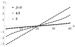
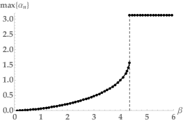
Figure 1: Exact eigenvalues for $N=40$, $M=4$ and three values of $\beta$ well below, just below and just above the transition. The right graph represents the plot of the maximal eigenvalue that demonstrates that it jumps at a certain temperature from a value $\simeq{\pi\over 2}$ to $\pi$.

4.4.2 Exact solution for the eigenvalue density at large $N$

The features observed in the numerical analysis may be explained analytically as follows. Let us return to the stationary point condition in eq. (58) expressing it in terms of $\rho(\alpha)$:

$$\!\!\!\!\int d\alpha^{\prime}\,\rho(\alpha^{\prime})\,\cot{\textstyle\frac{\alpha-\alpha^{\prime}}{2}}=6N\sum^{\infty}_{m=1}\,z_{\Phi}(x^{m})\int d\alpha^{\prime}d\alpha^{\prime\prime}\,\rho(\alpha^{\prime})\,\rho(\alpha^{\prime\prime})\,\sin\big{[}m\,(\alpha+\alpha^{\prime}+\alpha^{\prime\prime})\big{]}.$$ (74)

Let us assume that $\rho$ is symmetric and supported on $(-\alpha_{0},\alpha_{0})$ and thus write (74) as

$$\int d\alpha^{\prime}\,\rho(\alpha^{\prime})\,\cot{\textstyle\frac{\alpha-\alpha^{\prime}}{2}} =6\,N\,\sum^{\infty}_{m=1}\,z_{\Phi}(x^{m})\,\int d\alpha^{\prime}\,d\alpha^{\prime\prime}\,\rho(\alpha^{\prime})\,\rho(\alpha^{\prime\prime})\,\sin(m\,\alpha)\,\cos\big{[}m\,(\alpha^{\prime}+\alpha^{\prime\prime})\big{]}$$

$$=2\,\sum^{\infty}_{m=1}a_{m}\,\rho_{m}^{2}\,\sin(m\,\alpha),$$ (75)

where

$$a_{m}=3\,N\,z_{\Phi}(x^{m}),\qquad\qquad\rho_{m}=\int d\alpha\,\rho(\alpha)\,\cos(m\,\alpha).$$ (76)

Eq. (4.4.2) is same as eq. (5.20) of Aharony:2003sx and thus its solution may be written as

$$\rho(\alpha) ={\textstyle\frac{1}{\pi}\,\sqrt{\sin^{2}\frac{\alpha_{0}}{2}-\sin^{2}\frac{\alpha}{2}}\ }\sum_{k=1}^{\infty}Q_{k}\,\cos\big{[}(k-\tfrac{1}{2})\,\alpha\big{]},$$ (77)

$$Q_{k} =2\,\sum_{\ell=0}^{\infty}a_{k+\ell}\,\rho^{2}_{k+\ell}\,P_{\ell}(\cos\alpha_{0}),$$ (78)

where $P_{\ell}$ is the Legendre polynomial. To simplify the presentation, let us first consider a model with just one harmonic $\rho_{1}$ present in the r.h.s. of (4.4.2) which should be a good approximation for large $\beta$ when $x=e^{-\beta}\ll 1$ and thus the value of $a_{m}$ in (76) decreases with $m$. Then

$$\rho(\alpha)=\textstyle\frac{2}{\pi}\,a_{1}\,\rho_{1}^{2}\,\sqrt{\sin^{2}\frac{\alpha_{0}}{2}-\sin^{2}\frac{\alpha}{2}}\ \cos\frac{\alpha}{2}.$$ (79)

We still need to impose the self-consistency equations

$$\int_{-\alpha_{0}}^{\alpha_{0}}d\alpha\,\rho(\alpha)=1,\qquad\qquad\int_{-\alpha_{0}}^{\alpha_{0}}d\alpha\,\rho(\alpha)\,\cos\alpha=\rho_{1}.$$ (80)

We then find

$$2\,a_{1}\,\rho_{1}^{2}\,u=1,\qquad\qquad\qquad 2\,a_{1}\,\rho_{1}^{2}\,u\,(1-\tfrac{1}{2}\,u)=\rho_{1}\ ,\qquad u\equiv\sin^{2}\tfrac{\alpha_{0}}{2}\in(0,1)$$ (81)

$$1-\tfrac{1}{2}u=(2\,a_{1}\,u)^{-1/2}\ ,\qquad\qquad a_{1}=3N\,z_{\Phi}(e^{-\beta})\ .$$ (82)

Thus $u$ solves a cubic equation. For large $a_{1}$ we get a consistent solution

$$u=\frac{1}{2\,a_{1}}+\frac{1}{4\,a_{1}^{2}}+\dots\quad\rightarrow\quad\alpha_{0}=\big{[}\tfrac{3}{2}N\,z_{\Phi}(e^{-\beta})\big{]}^{-1/2}+\dots.$$ (83)

As $a_{1}$ decreases, we find a solution with $u\in(0,1)$ only up to the point

$$a_{1}=\frac{27}{16}\ ,\qquad{\rm i.e.}\qquad u=\frac{2}{3}\ .$$ (84)

This limiting value corresponds to the maximal width of the interval being

$$\alpha_{0}=2\,\arctan\sqrt{2}\ \simeq\ 0.6\,\pi.$$ (85)

To summarize, including just one harmonic in the sum in (4.4.2), for each temperature and $N$ such that

$$N\,z_{\Phi}(e^{-\beta})>\frac{9}{16}\ ,$$ (86)

we get the eigenvalue distribution

$$\rho(\alpha)=\begin{cases}\frac{1}{\pi\,\sin^{2}\frac{\alpha_{0}}{2}}\,\sqrt{u-\sin^{2}\frac{\alpha}{2}}\,\cos\frac{\alpha}{2}\ ,&\ \ \ |\alpha|<\alpha_{0}\\ 0\ &\ \ \ \alpha_{0}<|\alpha|\leq\pi\end{cases}$$ (87)

where $u=\sin^{2}\frac{\alpha_{0}}{2}$ is determined by the relation (82), i.e.

$$\tfrac{3}{2}\,u\,(2-u)^{2}=\big{[}N\,z_{\Phi}(e^{-\beta})\big{]}^{-1}.$$ (88)

For $\frac{9}{16}<N\,z_{\Phi}(e^{-\beta})<\frac{2}{3}$ there are two solutions $u_{1},u_{2}$ with $0<u_{1}<u_{2}<1$. Here $u_{1}$ is a minimum of the action, while $u_{2}$ is a local maximum, see Appendix C.2. A numerical test of (88) is shown in Fig. 2 where we compare its prediction with the edge of the exact eigenvalue distribution at $N=40$ found by taking just one harmonic in the potential term in (54).

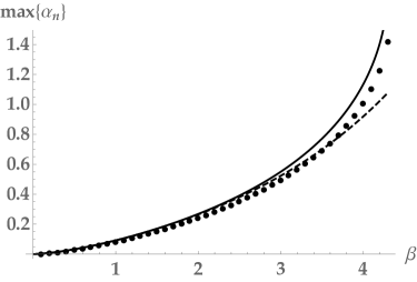
Figure 2: Comparison between the edge of the exact eigenvalue distribution at $N=40$ in the case of one harmonic in the potential term in (58) (solid circles) with the solution of (88) (solid line). We also show the high temperature approximation (92) in the one-harmonic case (dashed line).

Including up to $M$ higher harmonics, the equations (81) are replaced by similar ones involving $u$ and $\rho_{1},\dots,\rho_{M}$. The solution depends on $N$ and $\beta$ through the combinations $a_{m}=3N\,z_{\Phi}(e^{-m\,\beta})$, $\ m=1,\dots,M$ (see (4.4.2),(76)). For large $N$, the critical inverse temperature $\beta_{c}(N,M)$ admits a finite limit that may, in principle, depend on $M$. In fact, $a_{c}$ defined as

$$a_{c}(M)\equiv\lim_{N\to\infty}3N\,z_{\Phi}(e^{-\beta_{c}(N,M)})\ .$$ (89)

is independent of $M$. To see why, consider, for example, $z_{\Phi}(x)={x(1+x)\over(1-x)^{3}}$ corresponding to 4d scalar theory. If we solve $a_{c}=3N\,z_{\Phi}(e^{-\beta_{c}})$ for $\beta_{c}$ at large $N$, we get $\beta_{c}=-\log{a_{c}\over 3N}+{4\,a_{c}\over 3N}-{5\,a_{c}^{2}\over 3N^{2}}+\dots$. The coupling parameters $a_{m}=3N\,z_{\Phi}(e^{-m\beta})$ for higher harmonics in (4.4.2),(76) are then subleading, e.g., $3N\,z_{\Phi}(e^{-2\,\beta_{c}})={a_{c}^{2}\over 3N}-{8\,a_{c}^{3}\over 9N^{2}}+\dots$, and in general $3N\,z_{\Phi}(e^{-m\,\beta_{c}})={a_{c}^{m}\over(3N)^{m-1}}+\dots$. Thus,

$$a_{c}=a_{c}(M=1)=\frac{27}{16}\ ,$$ (90)

which is the value of $a_{1}$ found in (84).

To give an example, with $M=3$ harmonics and taking $N=50,60,\dots,100$ we get

$$\begin{array}[]{ccccccc}\hline\cr\hline\cr N&50&60&70&80&90&100\\ \hline\cr N\,z_{\Phi}(e^{\beta_{c}(N,M=3)})&0.562392&0.562409&0.562421&0.56243&0.562438&0.562444\\ \hline\cr\hline\cr\end{array}$$ (91)

A quadratic fit with $1/N$ and $1/N^{2}$ corrections gives $a_{c}(M=3)=3\times 0.562502$ which is equal to $27\over 16$ in (90) with a $10^{-6}$ relative precision.

As we will show in Appendix C.3, deep into the high temperature phase, the 1-harmonic result (83) is replaced by

$$\alpha_{0}=\Big{[}\tfrac{3}{2}\,N\,\sum_{m=1}^{\infty}m\,z_{\Phi}(e^{-m\,\beta})\Big{]}^{-1/2}+\dots$$ (92)

Similar results are found in the case when the general 3-plet representation is replaced by the symmetric or antisymmetric one: as we will show in Appendix C.4, the large $N$ behaviour is the same in all of these cases.

5 Concluding remarks

In this paper we discussed singlet partition function $Z$ of conformal theories defined by free fields in higher representations of an internal symmetry group. We observed that starting with rank 3 tensor case the number of singlet states grows so fast with the energy that the small temperature expansion of $Z$ has zero radius of convergence in the $N=\infty$ limit. This is reflected in the vanishing of the critical temperature $T_{c}$ at $N=\infty$. For large but finite $N$ there are two phases: $T<T_{c}$ and $T>T_{c}$, with $\log Z\sim N^{2}$ in the higher temperature phase (same scaling as found in the vector and adjoint representation cases).

We have concentrated on the case of the $p$-fundamental representation of $U(N)$ but similar conclusions are true also for the $[U(N)]^{p}$ invariant singlet partition function of $p$-tensors with inequivalent indices (see Appendix F). The same qualitative behaviour is found also when $U(N)$ symmetry is replaced by $O(N)$ (cf. Appendix D).

One open question is about possible implications for the AdS dual of the free $p$-plet or $p$-tensor CFT. The rich spectrum of singlet operators implies the presence of infinite sequences of massive fields in AdS (suggestive of a "tensionless membrane" spectrum in the $p=3$ case). It would be interesting to shed further light on this by studying simplest correlation functions of operators like $\overline{\phi}_{ijk}\phi_{ijk}$ (dual to a scalar in AdS) by generalizing the discussion of the vector and adjoint cases in Amado:2016pgy .

For the fields in the vector and adjoint representations the large $N$ free energy or 1-loop $\log Z$ of all higher spin fields in thermal AdS scales as $\mathcal{O}(N^{0})$ and matches the corresponding boundary CFT free energy in the low-temperature phase in (17), (19). In the high temperature phase the boundary CFT free energy is $\mathcal{O}(N^{2})$; that formally agrees with an AdS black-hole scaling in the adjoint case Witten:1998qj ; Witten:1998zw . In the vectorial case where $T_{c}$ grows with $N$ and thus the high temperature phase is not obviously attainable, a possibility of similar matching remains an open question Shenker:2011zf (the classical AdS action here scales as $N$ and thus a classical thermal object would contribute $\mathcal{O}(N)$ to the free energy).

In the 3-plet case the 1-loop partition function in thermal AdS computed for the full spectrum of fields dual to singlet conformal operators in the large $N$ limit should also be expected to be given by an asymptotic series matching the low temperature phase expression for $\log Z(x)=\mathcal{O}(N^{0})$ in (46). The high temperature phase result $\log Z(x)=\mathcal{O}(N^{2})$ here appears to be subleading to any potential contribution coming from a classical AdS action as that should scale as $\mathcal{O}(N^{3})$ (the coefficient in front of the AdS action should be $N^{3}$ to match the correlation functions in the free 3-plet CFT Bastianelli:1999ab ).

Another important question is how these conclusions may change in an interacting CFT, e.g., whether $T_{c}$ may become finite at a non-trivial large $N$ fixed point. This is of particular interest in the case of the $(2,0)$ tensor multiplet theory in 6d that should have an AdS₇ dual with a supergravity limit in the $N\to\infty$ limit admitting black holes and thus predicting $N^{3}$ scaling of the free energy kt1 ; Gubser:1998nz .

Appendix A $N=\infty$ partition function for 2-plet representation of $U(N)$

In addition to the adjoint representation $N\otimes\overline{N}$ one may consider also another rank 2 tensor representation – $N\otimes N$ or 2-plet of $U(N)$. The corresponding real representation in (10) is $R=N\otimes N+\overline{N}\otimes\overline{N}$ and thus $\chi_{R}(U)=[{\rm tr}\,(U)]^{2}+[{\rm tr}\,(U^{-1})]^{2}$ (see (13)). The resulting potential in (54) is then (cf. (55)–(57))

$$V^{\text{2-plet}}(\rho)=2\,N^{2}\,\int d\alpha\,d\alpha^{\prime}\rho(\alpha)\,\rho(\alpha^{\prime})\,\sum^{\infty}_{m=1}c_{m}\,\cos\big{(}m\,(\alpha+\alpha^{\prime})\big{)}.$$ (93)

In terms of the Fourier coefficients $\rho_{m}^{\pm}$ in (66) we get

$$V^{\text{2-plet}}=2\sum_{m=1}^{\infty}c_{m}\,[(\rho_{m}^{+})^{2}-(\rho_{m}^{-})^{2}].$$ (94)

As in the adjoint case (71),(72), integrating over $\rho_{m}^{\pm}$ we get for the $N=\infty$ partition function

$$\log Z^{\text{2-plet}}=-\frac{1}{2}\,\sum_{m=1}^{\infty}\log\big{(}1-\big{[}\,2\,z_{\Phi}(x^{m})\big{]}^{2}\big{)}\ ,$$ (95)

in agreement with (43). The corresponding single-trace partition function is given in (159). The expression (95) is valid in the low temperature phase, i.e. for temperatures below the critical one where $2\,z_{\Phi}(x_{c})\sim 1$.

For the symmetric 2-plet representation where $R=(N\otimes N)_{\rm sym}+(\overline{N}\otimes\overline{N})_{\rm sym}$ and

$$\chi_{R}(U)=\frac{1}{2}\big{[}\,\text{tr}(U)\big{]}^{2}+\frac{1}{2}\,\text{tr}(U^{2}),$$ (96)

we get instead of (93)

$$V^{\text{2-plet}^{+}} =N^{2}\int d\alpha\,d\alpha^{\prime}\rho(\alpha)\,\rho(\alpha^{\prime})\,\sum^{\infty}_{m=1}c_{m}\,\cos(m\,(\alpha+\alpha^{\prime}))+N\int d\alpha\,\rho(\alpha)\,\sum^{\infty}_{m=1}c_{m}\,\cos(2m\,\alpha)$$

$$=\,\sum_{m=1}^{\infty}c_{m}\,\big{[}(\rho_{m}^{+})^{2}-(\rho_{m}^{-})^{2}\big{]}+\,\sum_{m=1}^{\infty}c_{m}\,\rho_{2m}^{+}.$$ (97)

Adding this to (67) and performing again the Gaussian integration over $\rho^{\pm}$ gives (cf. (72),(95))

$$\log Z^{\text{2-plet}^{+}}=-\frac{1}{2}\,\sum_{m=1}^{\infty}\log\big{(}1-\big{[}z_{\Phi}(x^{m})\big{]}^{2}\big{)}+\frac{1}{2}\sum^{\infty}_{m=1}\frac{1}{m}\,\frac{\big{[}z_{\Phi}(x^{m})\big{]}^{2}}{1-z_{\Phi}(x^{2m})}\ .$$ (98)

In the antisymmetric 2-plet representation case there is a relative minus sign in (96) and thus in the last term in (A) but the final result for $Z$ is again the same as (98).

Appendix B Finite $N$ low temperature expansion of 3-plet partition function

Here we will supplement the large $N$ analysis in section 3 with a discussion of the finite $N$ case. At finite $N$, the low temperature expansion of the partition function may still be done by direct expanding (10). However, simple expressions like (22) or factorization leading to (38) are no longer valid. Instead, the group integrals (20) must be computed on a case by case basis.

In particular, for a 4d scalar in 3-plet representation, one can compute the following first five terms in the small $X$ expansion of $Z^{\text{3-plet}}_{{\rm S},4}$ for the increasing $N$ (the coefficients that are stable under the increase of $N$ are in bold face)

$$\begin{array}[]{ll}\hline\cr\hline\cr N&\qquad\qquad\qquad Z^{\text{3-plet}}_{{\rm S},4}\\ \hline\cr 2&1+5\,x^{2}+40\,x^{3}+212\,x^{4}+1080\,x^{5}+6054\,x^{6}+\cdots\\ 3&1+\bm{6}\,x^{2}+\bm{48}\,x^{3}+342\,x^{4}+2688\,x^{5}+21408\,x^{6}+\cdots\\ 4&1+\bm{6}\,x^{2}+\bm{48}\,x^{3}+387\,x^{4}+3384\,x^{5}+31765\,x^{6}+\cdots\\ 5&1+\bm{6}\,x^{2}+\bm{48}\,x^{3}+\bm{396}\,x^{4}+\bm{3504}\,x^{5}+35012\,x^{6}+\cdots\\ 6&1+\bm{6}\,x^{2}+\bm{48}\,x^{3}+\bm{396}\,x^{4}+\bm{3504}\,x^{5}+35535\,x^{6}+\cdots\\ 7&1+\bm{6}\,x^{2}+\bm{48}\,x^{3}+\bm{396}\,x^{4}+\bm{3504}\,x^{5}+\bm{35580}\,x^{6}+\cdots\\ \hline\cr\hline\cr\end{array}$$ (99)

The expansions in (99) may be derived using the character expansion method that is quite convenient at relatively small $N$ (see, e.g., Balantekin:1983km ). Irreducible representations of $U(N)$ may be labeled by $N$ integers $\bm{n}=(n_{1},n_{2},\dots,n_{N})$ with $n_{1}\geq n_{2}\geq\cdots\geq n_{N}\geq 0$. Denoting by $t_{1},\dots,t_{N}$ the eigenvalues of the group element $U$ in the fundamental representation, we obtain the character $\chi_{\bm{n}}$ from the Weyl formula ($i,j$ are row and column indices)

$$\chi_{\bm{n}}(U)=\frac{\det(t_{i}^{n_{j}+N-j})}{\det(t_{j}^{N-i})}\ .$$ (100)

This is a polynomial in the eigenvalues $t_{i}$ with total degree equal to $\sum_{i}n_{i}$. Any polynomial built out of powers of traces $\text{tr}(U^{k})$ may be expanded as a finite sum of such characters. Then the group integrals in (20) are easily evaluated by exploiting the orthonormality of the characters $\int dU\,\chi_{\bm{n}}(U)\,\overline{\chi_{\bm{n}^{\prime}}(U)}=\delta_{\bm{n},\bm{n}^{\prime}}$. The dependence on $N$ of the final result is a consequence of the fact that the fine details of the character decomposition also depend on $N$. To give a simple nontrivial example, let us consider the integral

$$I_{N}=\int dU\,|(\text{tr}\,U^{2})^{2}|^{2},\qquad U\in U(N),$$ (101)

The character expansion of $(\text{tr}U^{2})^{2}=(\sum_{i=1}^{N}t_{i}^{2})^{2}$ reads

$$\begin{array}[]{ll}\hline\cr\hline\cr N&(\text{tr}\,U^{2})^{2}\\ \hline\cr 2&2\,\chi_{22}-\chi_{31}+\chi_{40}\\ 3&2\,\chi_{220}-\chi_{310}+\chi_{400}-\chi_{211}\\ 4&2\,\chi_{2200}-\chi_{3100}+\chi_{4000}-\chi_{2110}+\chi_{1111}\\ 5&2\,\chi_{22000}-\chi_{31000}+\chi_{40000}-\chi_{21100}+\chi_{11110}\\ 6&2\,\chi_{220000}-\chi_{310000}+\chi_{400000}-\chi_{211000}+\chi_{111100}\\ \hline\cr\hline\cr\end{array}$$ (102)

and so on. Thus the cases $N=2,3$ are special, but there is a stable pattern for $N\geq 4$. Using the orthogonality of the characters and (102) we find for (101)

$$I_{2}=2^{2}+2\times 1^{2}=6,\qquad I_{3}=2^{2}+3\times 1^{2}=7,\qquad I_{N\geq 4}=2^{2}+4\times 1^{2}=8.$$ (103)

Appendix C Details of analysis of large $N$ partition function for 3-plet representation

C.1 $U(2)$ case

To compare the large $N$ and the finite $N$ cases, it is useful to consider the lowest non-trivial value of $N=2$. Then the action (54) in 3-plet case with just one harmonic included is a function of the single eigenvalue angle $\alpha=\alpha_{1}=-\alpha_{2}$ and inverse temperature $\beta$

$$S=-\log\sin^{2}\alpha-16\,z_{\Phi}(e^{-\beta})\,\cos^{3}\alpha\ .$$ (104)

The left part of Fig. 3 is the plot of this function for four values of $\beta$. For $\beta<\beta_{c}$ the value of $S$ at the global minimum is negative. This global minimum on the left and the local minimum at $\pi/2$ on the right become degenerate at $\beta_{c}$. For $\beta>\beta_{c}$ the global minimum is on the right at $\alpha=\pi/2$.

The transition temperature can be found analytically to be $\beta_{c}=2.454$. The associated eigenvalue is $\alpha_{c}=0.752$. This means that there is a first order (discontinuous) transition. Increasing $\beta$, the eigenvalue $\alpha$ goes from 0 to $\alpha_{c}$ and then jumps to $\alpha=\pi/2$. Increasing the number of harmonics included in (54) does not change this picture qualitatively. This is illustrated in the right plot in Fig. 3 where we assumed that there are 10 harmonics in (54).

What changes at higher $N$ is that the right minimum shifts further to the right, tending to $\alpha=\pi$ for $N\to\infty$.

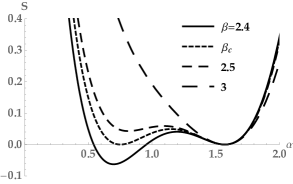
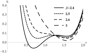
Figure 3: The action $S$ in (54) for the $U(2)$ theory as a function of the eigenvalue $\alpha=\alpha_{1}=-\alpha_{2}$. The left plot is for one and the right plot is for ten harmonics included in (54).

C.2 One-harmonic solution: value of the action for the eigenvalue density

To determine the leading term in the free energy $\log Z$ at the large $N$ saddle point one is to compute the value of the action (60) on the solution of (74).

Below we shall compute the sum of the two terms in the action (60)

$$S_{M} =-\frac{1}{2}N^{2}\int d\alpha\,d\alpha^{\prime}\,\rho(\alpha)\,\rho(\alpha^{\prime})\textstyle\,\log\sin^{2}\frac{\alpha-\alpha^{\prime}}{2},$$ (105)

$$V =-2\,N^{3}\,z_{\Phi}(e^{-\beta})\,\int d\alpha\,d\alpha^{\prime}\,d\alpha^{\prime\prime}\,\rho(\alpha)\,\rho(\alpha^{\prime})\,\rho(\alpha^{\prime\prime})\,\cos(\alpha+\alpha^{\prime}+\alpha^{\prime\prime})$$ (106)

on the solution (79) found in one-harmonic approximation, i.e.

$$\rho(\alpha)=\frac{1}{u\,\pi}\,\sqrt{u-\sin^{2}\frac{\alpha}{2}}\,\cos\frac{\alpha}{2},\qquad\qquad u=\sin^{2}\frac{\alpha_{0}}{2}.$$ (107)

Using the identity

$$-\frac{1}{2}\log\sin^{2}\frac{\alpha}{2}=\log 2+\sum_{m=1}^{\infty}\frac{1}{m}\cos(m\,\alpha),$$ (108)

we find for the measure term

$$S_{M}=-\frac{1}{2}N^{2}\int d\alpha\,d\alpha^{\prime}\,\rho(\alpha)\,\rho(\alpha^{\prime})\,\log\sin^{2}\tfrac{\alpha-\alpha^{\prime}}{2}=N^{2}\,\Big{(}\log 2+\sum_{m=1}^{\infty}\frac{1}{m}\,\rho_{m}^{2}\Big{)},$$ (109)

where $\rho_{m}$ was defined in (76), i.e.

$$\rho_{m}=\frac{1}{\pi\,u}\,\int_{-\alpha_{0}}^{\alpha_{0}}d\alpha\sqrt{u-\sin^{2}\frac{\alpha}{2}}\,\cos\frac{\alpha}{2}\,\cos(m\alpha),\qquad u=\sin^{2}\frac{\alpha_{0}}{2}\ .$$ (110)

Introducing $t=\sin\frac{\alpha}{2}/\sin\frac{\alpha_{0}}{2}$ we get

$$\rho_{m}=\frac{2}{\pi\,\sqrt{u}}\,\int_{0}^{1}dt\,\sqrt{1-t^{2}}\sqrt{1-u\,t^{2}}\,\cos\big{[}2\,m\,\arcsin(u\,t)\big{]}.$$ (111)

Using the expansion

$$\cos\big{[}2\,m\,\arcsin(u\,t)\big{]}=\sum_{n=0}^{\infty}\frac{(m)_{n}(-m)_{n}}{(2n)!}\,(2\,u\,t)^{2n},$$ (112)

we obtain from (111)

$$\rho_{m}=\sum_{n=0}^{m}\frac{(m)_{n}\,(-m)_{n}}{n!\,(n+1)!}\,u^{n}={}_{2}F_{1}(-m,m,2;u).$$ (113)

Thus

$$S_{M}=N^{2}\,\Big{(}\log 2+\sum_{m=1}^{\infty}\frac{1}{m}\,\big{[}{}_{2}F_{1}(-m,m,2;u)\big{]}^{2}\Big{)}\ .$$ (114)

The potential term is given simply by

$$V=-2\,N^{3}\,z_{\Phi}(e^{-\beta})\,\rho_{1}^{3}=-2\,N^{3}\,z_{\Phi}(e^{-\beta})\,\big{(}1-\tfrac{u}{2}\big{)}^{3}\equiv N^{2}\bar{V}(u)\ ,$$ (115)

where we used (81),(82).

In Fig. 4 we plot $S_{M}$ and $V$ evaluated as functions of $u$ at $a_{1}=3\,N\,z_{\Phi}(e^{-\beta})=4$, i.e. at the value which is above the bound in (84). As expected, there is a minimum of the total action $S=S_{M}+V$ located at the value predicted by the cubic equation for $u$ in (82).

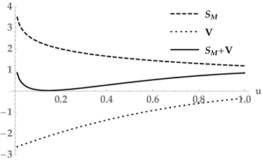
Figure 4: Plot of the measure term $S_{M}$ in (109) and the potential term $V$ in (115) in the eigenvalue density action at $a_{1}=3\,N\,z_{\Phi}(e^{-\beta})=4$. The black line is the total action that has a minimum at the position predicted by (82), i.e. at $u\simeq 0.145$.

C.3 Including higher harmonics

It is easy to generalize the discussion in section 4.4.2 to the case of higher harmonics included in (4.4.2). Some analytical information may be obtained at least for small $\beta$ where the maximal value of eigenvalues $\alpha_{0}$ is small. We need to solve eq. (74), i.e.

$$\!\!\!\!\int d\alpha^{\prime}\,\rho(\alpha^{\prime})\,\cot\tfrac{\alpha-\alpha^{\prime}}{2}=6N\sum_{m=1}^{\infty}\,z_{\Phi}(x^{m})\int d\alpha^{\prime}\,d\alpha^{\prime\prime}\,\rho(\alpha^{\prime})\,\rho(\alpha^{\prime\prime})\,\sin(m\,(\alpha+\alpha^{\prime}+\alpha^{\prime\prime})).$$ (116)

Introducing

$$\theta={\alpha\over\alpha_{0}}\ ,\qquad\widetilde{\rho}(\theta)=\alpha_{0}\,\rho(\alpha_{0}\,\theta)\ ,\qquad d\alpha\,\rho(\alpha)=d\theta\,\widetilde{\rho}(\theta)\ ,\qquad\int_{-1}^{1}d\theta\,\widetilde{\rho}(\theta)=1$$ (117)

and expanding (116) in small $\alpha_{0}$, we obtain at the leading order

$$\int_{-1}^{1}d\theta^{\prime}\,\frac{\widetilde{\rho}(\theta^{\prime})}{\theta-\theta^{\prime}}-3\,N\,\alpha_{0}^{2}\,\sum_{m=1}^{\infty}m\,z_{\Phi}(e^{-m\,\beta})\,\theta=0\ .$$ (118)

For a constant parameter $\gamma$, the Hilbert problem

$$\int_{-1}^{1}d\theta^{\prime}\,\frac{\widetilde{\rho}(\theta^{\prime})}{\theta-\theta^{\prime}}=\gamma\,\theta,\qquad\qquad\theta\in(-1,1)$$ (119)

has the unique solution

$$\widetilde{\rho}(\theta)=\frac{\gamma}{\pi}\,\sqrt{1-\theta^{2}}.$$ (120)

The normalization in (117) fixes $\gamma=2$. Comparing with (118), we thus determine

$$\alpha_{0}=\Big{[}\tfrac{3}{2}\,N\,\sum_{m=1}^{\infty}m\,z_{\Phi}(e^{-m\,\beta})\Big{]}^{-1/2}.$$ (121)

For one-harmonic case, this gives $\alpha_{0}=\big{[}\frac{3}{2}N\,z_{\Phi}(e^{-\beta})\big{]}^{-1/2}$ or $u=1/(6\,N\,z_{\Phi})+\dots$, in agreement with (83).

C.4 Eigenvalue density for (anti) symmetric 3-plet representation

We can repeat the analysis of section 4 for the (anti) symmetric 3-plet representation, see (14). Here the action is (54) with

$${\mathcal{V}}^{\pm}(\bm{\alpha})=\frac{1}{3}\,\sum_{ijk}\cos(\alpha_{i}+\alpha_{j}+\alpha_{k})\pm\sum_{ij}\cos(\alpha_{i}+2\,\alpha_{j})+\frac{2}{3}\sum_{i}\cos(3\,\alpha_{i}).$$ (122)

The stationary-point equation for the eigenvalues $\alpha_{i}$ is

$$\sum_{j\neq i}\cot\tfrac{\alpha_{i}-\alpha_{j}}{2}-\sum^{\infty}_{m=1}z_{\Phi}(e^{-m\beta})\,\Big{[} \sum_{jk}\sin(m(\alpha_{i}+\alpha_{j}+\alpha_{k}))\pm\sum_{j}\sin(m(\alpha_{i}+2\,\alpha_{j}))$$

$$\pm 2\,\sum_{j}\sin(m(2\,\alpha_{i}+\alpha_{j}))+2\,\sin(3\,m\,\alpha_{i})\Big{]}=0.$$ (123)

Written in terms of the density of eigenvalues (59), this becomes

$$\int d\alpha^{\prime}\,\rho(\alpha^{\prime})\,\cot\tfrac{\alpha-\alpha^{\prime}}{2}=\sum^{\infty}_{m=1}z_{\Phi}(e^{-m\,\beta})\,\Big{[}N\,\int d\alpha^{\prime}\,\int d\alpha^{\prime\prime}\,\rho(\alpha^{\prime})\,\rho(\alpha^{\prime\prime})\,\sin(m(\alpha+\alpha^{\prime}+\alpha^{\prime\prime}))$$

$$\pm\int d\alpha^{\prime}\,\rho(\alpha^{\prime})\,\sin(m(\alpha+2\,\alpha^{\prime}))\pm 2\,\int d\alpha^{\prime}\,\rho(\alpha^{\prime})\,\sin(m(2\,\alpha+\alpha^{\prime}))+\frac{2}{N}\,\sin(3\,m\,\alpha)\Big{]}.$$ (124)

Comparing to (74) found in the general 3-plet case we observe that the additional terms appearing in the (anti) symmetric case are suppressed at large $N$ by powers of $1/N$.

In more detail, in the simple one-harmonic case, we can write (C.4) in the form of (4.4.2),(76)

$$\int d\alpha^{\prime}\,\rho(\alpha^{\prime})\,\cot\tfrac{\alpha-\alpha^{\prime}}{2}=2\,\sum_{m=1}^{3}C_{m}\,\sin(m\,\alpha),$$ (125)

where

$$C_{1}=\frac{1}{2}\,(N\,\rho_{1}^{2}\pm\rho_{2})\,z_{\Phi},\qquad C_{2}=\pm\,z_{\Phi}\,\rho_{1},\qquad C_{3}=\frac{z_{\Phi}}{N},$$ (126)

and then the solution for the density is similar to (77),(78). Assuming that for $N\to\infty$ with $N\,z_{\Phi}$ fixed we have $\rho_{1},\rho_{2}$ finite, it is clear that the effects of (anti) symmetrization are subleading.

To check these assumptions, let us consider explicitly the symmetric representation case, i.e. the plus sign in (C.4),(126). Introducing $u=\sin^{2}\frac{\alpha_{0}}{2}$, the three self-consistency conditions obtained by plugging $\rho$ into the definition of $\rho_{1}$ and $\rho_{2}$ and also imposing $\int d\alpha\,\rho(\alpha)=1$ are

$$1 =\frac{2}{N}u\left(10u^{2}-12u+3\right)z_{\Phi}+N\rho_{1}^{2}u\,z_{\Phi}-u\,z_{\Phi}\left(-4\rho_{1}-\rho_{2}+6\rho_{1}u\right),$$

$$\rho_{1} =-\frac{1}{2}N\rho_{1}^{2}(u-2)uz_{\Phi}-\frac{3}{N}u(5u-2)(u-1)^{2}z_{\Phi}$$

$$\qquad+\frac{1}{2}uz_{\Phi}\left(8\rho_{1}+2\rho_{2}+8\rho_{1}u^{2}-16\rho_{1}u-\rho_{2}u\right),$$ (127)

$$\rho_{2} =\frac{6}{N}u\left(6u^{2}-4u+1\right)(u-1)^{2}z_{\Phi}+N\rho_{1}^{2}u(u-1)^{2}z_{\Phi}$$

$$\qquad-uz_{\Phi}\left(-4\rho_{1}-\rho_{2}+9\rho_{1}u^{3}-20\rho_{1}u^{2}-\rho_{2}u^{2}+14\rho_{1}u+2\rho_{2}u\right).$$

One may study the properties of the solution $(u,\rho_{1},\rho_{2})$ of the algebraic system (C.4) for fixed $z_{\Phi}$ and increasing $N$. A numerical analysis shows that for any $z_{\Phi}$ we find exactly one acceptable solution as soon as $N$ is sufficiently large. This solution may be expanded in powers of $1/N$ and reads

$$\qquad\qquad u=\frac{1}{Nz_{\Phi}}+\frac{1}{(Nz_{\Phi})^{2}}-{5\over N}\ \frac{1}{Nz_{\Phi}}+\dots,$$ (128)

$$\rho_{1}=1-\frac{1}{2Nz_{\Phi}}-\frac{1}{2(Nz_{\Phi})^{2}}+\frac{5}{2N}\ {1\over Nz_{\Phi}}+\dots,$$ (129)

$$\qquad\rho_{2}=1-\frac{1}{2Nz_{\Phi}}-\frac{1}{(Nz_{\Phi})^{2}}+\frac{10}{N}\ {1\over Nz_{\Phi}}+\dots\ .$$ (130)

Thus the large $N$ behaviour at fixed $Nz_{\Phi}$ is similar to the asymmetric 3-plet case, with $\alpha_{0}\sim(Nz_{\Phi})^{-1/2}$. If we fix $N$ and vary $z_{\Phi}$, the solution may develop branches and may exist only in certain ranges. One example is in Fig. 5 where we show the solution for $u$ as a function of $z_{\Phi}$ for $N=40$. There is a minimal value of $z_{\Phi}$ and also a narrow region where both branches are present. Completely similar features are observed in the case of the antisymmetric 3-plet representation.

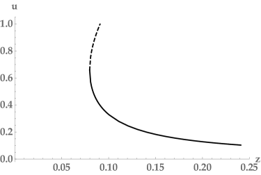
Figure 5: Solution of the system (C.4) for $u$ as a function of variable $z\equiv z_{\Phi}$ for $N=40$.

Appendix D $N=\infty$ limit of low temperature expansion of $O(N)$ partition function

If the symmetry group is $O(N)$, we may again start with the general expression for the partition function in (10). Renaming matrix $U$ as $M\in O(N)$, the characters of the relevant representations $R$ are

$$\begin{array}[]{ccc}\hline\cr\hline\cr R&&\chi_{R}\\ \hline\cr\hline\cr{\rm vector}:N&\phantom{\qquad}&\text{tr}(M)\\ {\rm adjoint}:(N\otimes N)_{A}&&\frac{1}{2}\,\text{tr}(M)^{2}-\frac{1}{2}\,\text{tr}(M^{2})\\ \text{3-plet}:N^{\otimes 3}&&\text{tr}(M)^{3}\\ \hline\cr\hline\cr\end{array}$$ (131)

Expanding (10) in powers of the matrix $M$, we are led to the problem of computing the $O(N)$ group integrals parametrized by the integers $\bm{a}=\{a_{\ell}\}$

$$I(\bm{a})=\int dM\,\prod_{\ell\geq 1}(\text{tr}\,M^{\ell})^{a_{\ell}}\ .$$ (132)

As in the $U(N)$ case in (20), if $N$ is sufficiently large, $I(\bm{a})$ does not depend on $N$ and factorizes. The precise condition is $N\geq 2\,\kappa(\bm{a})$ where $\kappa(\bm{a})$ was defined in (21). In this case one can represent the integral in the form

$$I(\bm{a})=\int\prod_{\ell}\frac{d\xi_{\ell}}{\sqrt{2\pi}}\,e^{-\frac{1}{2}\xi_{\ell}^{2}}\ \prod_{\ell\geq 1}(\sqrt{\ell}\,\xi_{\ell}+\eta_{\ell})^{a_{\ell}}\ ,\qquad\qquad\textstyle\eta_{l}=\frac{1+(-1)^{\ell}}{2},$$ (133)

where $\xi_{\ell}$ are independent normal variables with Gaussian distribution pastur2004moments . As a result,

$$I(\bm{a})=\prod_{\ell\geq 1}\begin{cases}\frac{1+(-1)^{a_{\ell}}}{2}\,(2\,\ell)^{a_{\ell}/2}\,\frac{1}{\sqrt{\pi}}\Gamma(\frac{a_{\ell}+1}{2}),&\ \ \ \ell\ \text{odd},\\ \sum_{n=0}^{a_{\ell}}\binom{a_{\ell}}{n}\,\frac{1+(-1)^{n}}{2}\,(2\,\ell)^{n/2}\,\frac{1}{\sqrt{\pi}}\Gamma(\frac{n+1}{2}),&\ \ \ \ell\ \text{even}.\end{cases}$$ (134)

Using this result, we may determine the low temperature expansion of the partition function for a 4d scalar field transforming in various representations like in (131). In the vector representation case we get (cf. (24))

$$Z^{\text{vector}}_{{\rm S},4}=1+\,x^{2}+4\,x^{3}+20\,x^{4}+56\,x^{5}+164\,x^{6}+412\,x^{7}+1116\,x^{8}+\dots.$$ (135)

This agrees with the result of Giombi:2014yra for the large $N$ partition function in the $O(N)$ case which is given by (15) with the following "single-trace" partition function (cf. (17))

$$Z_{\rm s.t.}^{\text{vector}} =\textstyle\frac{1}{2}\,\big{[}z_{\Phi}(x)\big{]}^{2}+\frac{1}{2}\,z_{\Phi}(x^{2})$$

$$=\,x^{2}+4\,x^{3}+19\,x^{4}+52\,x^{5}+134\,x^{6}+280\,x^{7}+554\,x^{8}+984\,x^{9}+\dots.$$ (136)

In the adjoint scalar case, we find (cf. (25))

$$Z^{\text{adjoint}}_{{\rm S},4} =1+\,x^{2}+4\,x^{3}+21\,x^{4}+66\,x^{5}+235\,x^{6}+724\,x^{7}+2423\,x^{8}+7873\,x^{9}$$

$$\ \ \quad\ +26463\,x^{10}+88252\,x^{11}+297918\,x^{12}+1003530\,x^{13}+\dots,$$ (137)

with the corresponding single-trace partition function in (15) being

$$Z_{\rm s.t.}^{\text{adjoint}} =\,x^{2}+4\,x^{3}+20\,x^{4}+62\,x^{5}+204\,x^{6}+578\,x^{7}+1730\,x^{8}$$

$$\ \ \ \ \ +5073\,x^{9}+15495\,x^{10}+47791\,x^{11}+\dots\ .$$ (138)

$Z_{\rm s.t.}^{\text{adjoint}}$ counts the operators which are single traces of products of scalars fields which are antisymmetric $O(N)$ matrices. Here we have the identity

$$\text{tr}(\Phi_{1}\Phi_{2}\dots\Phi_{n})=(-1)^{n}\,\text{tr}(\Phi_{n}\Phi_{n-1}\dots\Phi_{1})\ ,$$ (139)

where $\Phi_{n}$ is the scalar $\varphi_{ij}=-\varphi_{ji}$ or any derivative of it. It seems non-trivial to apply Polya counting in the case of an additional constraint (139), and we did not find a simple closed formula for $Z_{\rm s.t.}$ like (18). To see the non-trivial effect of the constraint (139), let us explicitly list the single-trace operators up to dimension 5:

$$\begin{array}[]{ccc}\hline\cr\hline\cr\dim&\text{operator}&\text{multiplicity}\\ \hline\cr\hline\cr 2&\text{tr}(\varphi\varphi)&1\\ \hline\cr 3&\text{tr}(\varphi\partial_{\mu}\varphi)&4\\ \hline\cr 4&\text{tr}(\varphi\partial_{\mu}\partial_{\nu}\varphi)&9\\ &\text{tr}(\partial_{\mu}\varphi\partial_{\nu}\varphi)&10\\ &\text{tr}(\varphi\varphi\varphi\varphi)&1\\ \hline\cr 5&\text{tr}(\varphi\partial_{\mu}\partial_{\nu}\partial_{\rho}\varphi)&20-4=16\\ &\text{tr}(\partial_{\mu}\varphi\partial_{\nu}\partial_{\rho}\varphi)&4\times 9=36\\ &\text{tr}(\varphi\partial_{\mu}\varphi\partial_{\nu}\varphi)&6\ (\mu\neq\nu)\\ &\text{tr}(\varphi\varphi\varphi\partial_{\mu}\varphi)&4\\ \cline{2-3}\cr\end{array}$$ (140)

Note that $\text{tr}(\varphi\varphi\partial_{\mu}\partial_{\nu}\varphi)=0$ in view of (139). Also, $\text{tr}(\varphi\partial_{\mu}\varphi\partial_{\nu}\varphi)$ with $\mu=\nu$ is again zero in view of (139). The resulting multiplicities 1, 4, 20, 62 are in agreement with (D).

The case the symmetric representation $(N\otimes N)_{S}$ appears to be simpler. Here the analog of (139) reads

$$\text{tr}(\Phi_{1}\Phi_{2}\dots\Phi_{n})=\text{tr}(\Phi_{n}\Phi_{n-1}\dots\Phi_{1}),$$ (141)

and it adds an extra symmetry to the standard cyclic invariance of the trace. Then the total and single-trace partition functions are found to be

$$Z^{\text{2-plet}^{+}}_{{\rm S},4} =1+\,x+6\,x^{2}+20\,x^{3}+75\,x^{4}+246\,x^{5}+862\,x^{6}+2852\,x^{7}$$

$$\qquad+9643\,x^{8}+32040\,x^{9}+107141\,x^{10}+356651\,x^{11}+1191345\,x^{12}+\dots,$$ (142)

$$Z^{\text{2-plet}^{+}}_{\rm s.t.} =\,x+5\,x^{2}+14\,x^{3}+40\,x^{4}+101\,x^{5}+276\,x^{6}+715\,x^{7}$$

$$\qquad+1982\,x^{8}+5553\,x^{9}+16379\,x^{10}+49476\,x^{11}+154346\,x^{12}+\dots.$$ (143)

One can find a closed form of (D) using the Polya enumeration theorem and taking into account that the symmetry group is the cyclic group with an additional inversion (141). A careful examination of the cycle structure of the associated permutations gives

$$Z^{\text{2-plet}^{+}}_{\rm s.t.}= -\frac{1}{2}\,\sum_{m=1}^{\infty}\frac{\varphi(m)}{m}\,\log\big{(}1-z_{\Phi}(x^{m})\big{)}$$

$$+\frac{1}{2}\,\sum_{m=1}^{\infty}\sum_{\ell=1}^{k}\frac{1}{m}\,\begin{cases}\begin{cases}\big{[}z_{\Phi}(x^{2})\big{]}^{\frac{m}{2}}&\ell\ \text{even}\\ \big{[}z_{\Phi}(x^{2})\big{]}^{\frac{m}{2}-1}\,\big{[}z_{\Phi}(x)\big{]}^{2}&\ell\ \text{odd}\end{cases}&\qquad m\ \text{even}\\ \big{[}z_{\Phi}(x^{2})\big{]}^{\frac{m-1}{2}}\,z_{\Phi}(x)&\qquad m\ \text{odd}.\end{cases}$$ (144)

where $\varphi(m)$ is the same as in (18) and the additional $1/2$ factors are due to the fact that the symmetry group for a trace with $m$ objects is $2m$ (from $m$ shifts and $m$ reflected shifts).

Using (D), we have computed the series expansion (D) up to the very high order $\mathcal{O}(x^{100})$ and a numerical analysis revealed that the series is convergent for $x<x_{c}$ with $z_{\Phi}(x_{c})=1$ (for the 4d scalar this critical value is $x_{c}\simeq 0.285$). The same behaviour was found in the $U(N)$ case so the conclusion is that the additional terms in the second line of (D) do not worsen the convergence.

In the 3-plet case representation case we obtain (cf. (24))

$$Z^{\text{3-plet}}_{{\rm S},4} =1+11\,x^{2}+60\,x^{3}+773\,x^{4}+7920\,x^{5}+110781\,x^{6}+1509060\,x^{7}$$

$$\qquad+23807838\,x^{8}+379566780\,x^{9}+6645202174\,x^{10}+118587559020\,x^{11}$$

$$\qquad+2264713625957\,x^{12}+44204970285420\,x^{13}+\dots,$$ (145)

with the corresponding "single-trace" partition function being

$$Z_{\rm s.t.}^{\text{3-plet}}= 11\,x^{2}+60\,x^{3}+707\,x^{4}+7260\,x^{5}+100888\,x^{6}+1382820\,x^{7}+21944399\,x^{8}$$

$$+352168900\,x^{9}+6207336278\,x^{10}+111438968700\,x^{11}+\dots.$$ (146)

To reproduce the $x^{2}$ term here by counting dimension 2 operators we need to classify various bilinear contractions: (i) there are $\frac{1}{2}(3\times 4)=6$ contractions containing traces $\varphi_{iij}\varphi_{iij},\ \varphi_{iij}\varphi_{iji},\ \dots,$ where we need to account that position of the index contracted between the two fields matters and that there is a symmetry between the two fields in the real scalar case; (ii) there are also $3!$ irreducible contractions $\varphi_{ijk}\varphi_{ijk},\ \ \varphi_{ijk}\varphi_{ikj},\ \dots,$ but one needs to take into account the symmetry relation $\varphi_{ijk}\,\varphi_{jki}\equiv\varphi_{ijk}\,\varphi_{kij}$, so we are left with $6-1=5$ independent choices. The total $6+5=11$ matches the coefficient of the $x^{2}$ term in (145),(D).

There are fewer operators in the case of totally symmetric or antisymmetric 3-plet representations, i.e. the coefficients in the small $x$ expansion of $Z$ should be much smaller. Indeed, we find directly from (14) (cf. (3.2),(3.2))

$$Z^{\text{3-plet}^{+}}_{{\rm S},4}=1+ 2\,x^{2}+8\,x^{3}+46\,x^{4}+156\,x^{5}+668\,x^{6}+2684\,x^{7}+12044\,x^{8}$$

$$+53556\,x^{9}+249495\,x^{10}+1182524\,x^{11}+5780012\,x^{12}+\dots,$$ (147)

$$Z^{\text{3-plet}^{+}}_{\rm s.t.}= 2\,x^{2}+8\,x^{3}+43\,x^{4}+140\,x^{5}+542\,x^{6}+2036\,x^{7}+8688\,x^{8}$$

$$+37868\,x^{9}+175063\,x^{10}+832556\,x^{11}+4102153\,x^{12}+\dots,$$ (148)

$$Z^{\text{3-plet}^{-}}_{{\rm S},4}=1+ \,x^{2}+4\,x^{3}+22\,x^{4}+64\,x^{5}+228\,x^{6}+716\,x^{7}+2701\,x^{8}$$

$$+10104\,x^{9}+41897\,x^{10}+179420\,x^{11}+820244\,x^{12}+\dots,$$ (149)

$$Z^{\text{3-plet}^{-}}_{\rm s.t.}= \,x^{2}+4\,x^{3}+21\,x^{4}+60\,x^{5}+196\,x^{6}+568\,x^{7}+2002\,x^{8}$$

$$+7324\,x^{9}+30768\,x^{10}+136096\,x^{11}+644817\,x^{12}+\dots.$$ (150)

For example, the first few single-trace states in the antisymmetric case are

$$\begin{array}[]{ccc}\hline\cr\hline\cr\dim&\text{operator}&\text{multiplicity}\\ \hline\cr\hline\cr 2&\varphi_{ijk}\,\varphi_{ijk}&1\\ \hline\cr 3&\varphi_{ijk}\,\partial_{\mu}\varphi_{ijk}&4\\ \hline\cr 4&\varphi_{ijk}\,\partial_{\mu}\partial_{\nu}\varphi_{ijk}&9\\ &\partial_{\mu}\varphi_{ijk}\,\partial_{\nu}\varphi_{ijk}&10\\ &\varphi_{ijk}\,\varphi_{ijl}\varphi_{pqk}\varphi_{pql}&1\\ &\varphi_{ijk}\,\varphi_{ipq}\varphi_{jpl}\varphi_{kql}&1\\ \hline\cr\hline\cr\end{array}$$ (151)

As a final remark, we note that using the discussion in Giombi:2014yra providing the suitable modification of the measure term in (52) for the $O(N)$ case, it is possible also to study the large $N$ thermodynamics and the structure of phase transitions in this case, but there should be no qualitative changes compared to $U(N)$ case analyzed in section 4.

Appendix E General expression for single-trace partition function

Given the $N=\infty$ partition function $Z(x)$ one can invert the relation (15) and find the single-trace partition function $Z_{\rm s.t.}(x)$ that counts only irreducible ("single-trace") contractions among all singlet operators. This was already discussed in Gibbons:2006ij and here we present an equivalent but slightly more explicit version of this inverse relation.

Starting with the relation

$$L(x)=\sum_{m=1}^{\infty}\frac{1}{m}\,Z_{\rm s.t.}(x^{m}),\qquad\qquad L(x)\equiv\log Z(x)\ ,$$ (152)

we find

$$Z_{\rm s.t.}(x)=L(x)+\sum_{m\in\Omega}(-1)^{\nu_{m}}\,\frac{1}{m}\,L(x^{m})\ .$$ (153)

Here $\Omega=\{2,3,5,6,7,10,11,13,\dots\}$ is the set of so-called square-free integers, such that their prime number factorization is of the form $m=\prod_{i=1}^{\nu_{m}}p_{i}$, i.e. is the product of prime factors each appearing in the first power only. The sign factor $(-1)^{\nu_{m}}$ is known in this context as the Liouville function. The proof of (153) is by substituting (153) into (152):

$$\sum_{m=1}^{\infty}\frac{1}{m}\,Z_{\rm s.t.}(x^{m}) =\sum_{m=1}^{\infty}\frac{1}{m}\,L(x^{m})+\sum_{n=1}^{\infty}\sum_{q\in\Omega}(-1)^{\nu_{q}}\frac{1}{n\,q}L(x^{nq})$$

$$=\sum_{m=1}^{\infty}\frac{1}{m}\,L(x^{m})\Big{[}1+\mathop{\sum_{q\in\Omega}}_{q|m}(-1)^{\nu_{q}}\Big{]}=L(x)\ .$$ (154)

In the last equality, we used that

$$\mathop{\sum_{q\in\Omega}}_{q|m}(-1)^{\nu_{q}}=\begin{cases}1\ ,&\ \ m=1,\\ 0\ ,&\ \ m>1.\end{cases}$$ (155)

To prove (155), it is enough to observe that if $m>1$ is factorizable into $M$ powers of distinct primes, $m=p_{1}^{a_{1}}\cdots p_{M}^{a_{M}}$, then

$$1+\mathop{\sum_{q\in\Omega}}_{q|m}(-1)^{\nu_{q}}={\textstyle 1-M+\frac{M(M-1)}{2}-\frac{M(M-1)(M-2)}{3!}}+...=(1-1)^{M}=0,$$ (156)

where we used that the square-free integers $q$ dividing $m$ are of the form $p_{i}$, $p_{i}p_{j}\ (i\neq j)$, etc.

Let us note that if $L(x)$ in (152) has the form

$$L(x)=\sum_{m=1}^{\infty}f(x^{m})\ ,$$ (157)

where $f(x)$ is independent of $m$, then one can show that (153) gives

$$Z_{\rm s.t.}(x)=\sum_{m=1}^{\infty}\frac{\varphi(m)}{m}\,f(x^{m})\ ,$$ (158)

where $\varphi$ is the Euler’s totient function as in (18). One example is the adjoint representation case in (19). Another is the 2-plet representation with $Z$ given in (95) in which case (cf. (18))

$$Z^{\text{2-plet}}_{\rm s.t.}(x)=-{1\over 2}\sum_{m=1}^{\infty}\frac{\varphi(m)}{m}\,\log\big{(}1-4\big{[}\,z_{\Phi}(x^{m})\big{]}^{2}\big{)}\ .$$ (159)

Appendix F Singlet partition function of $[U(N)]^{p}$ invariant $p$-tensor theory

Given a free $p$-tensor $\Phi=(\varphi_{i_{1}...i_{p}})$ with each internal index running from from 1 to $N$ one may have several options of how to define the corresponding CFT and thus the associated singlet partition function $Z(x)$ (i.e. which singlet operators given by contractions of fields to include). In the main part of this paper we treated all $p$ indices of $(\varphi_{i_{1}...i_{p}})$ as equivalent and thus all of their contractions were allowed. The corresponding singlet partition function on $S^{1}_{\beta}\times S^{d-1}$ was then found by gauging the global $U(N)$ or $O(N)$ symmetry.

If instead all $p$ indices are assumed to be distinguishable as, e.g., in the interacting tensor models considered in Witten:2016iux ; Klebanov:2016xxf , then the singlet constraint may be implemented by gauging the full $[U(N)]^{p}$ symmetry group Klebanov:2016xxf . As we shall demonstrate below, in this case the low temperature expansion of $Z(x)$ will again diverge in the $N=\infty$ limit starting with the $p=3$ case, i.e. the critical temperature will vanish with $N\to\infty$ if $p\geq 3$.

The computation of the singlet partition function in the $[U(N)]^{p}$ invariant theory (that we will call "$p$-tensor" theory for short) turns out to be very similar to the case of the $U(N)$ invariant $p$-plet theory considered in sections 3 and 4 above. To compute $Z$ we may start with the path integral for $\varphi_{i_{1}...i_{p}}$ with covariant derivative containing $p$ independent flat gauge fields $A_{\mu}^{(r)}$ ($r=1,...,p$) and average over their $S^{1}$ holonomies, i.e. constant $N\times N$ hermitian $A_{0}^{(r)}$ matrices with the eigenvalues $\alpha_{ir}$, or, equivalently, over $U(N)$ matrices $U_{r}$ with eigenvalues $e^{i\alpha_{ir}}$ ($i=1,....,N;\ r=1,...,p$). As $\varphi_{i_{1}...i_{p}}$ transforms in the direct product of fundamental representations of $p$ copies of $U(N)$ group, the potentials $A_{0}^{(r)}$ or the eigenvalues $\alpha_{ir}$ simply sum up, i.e. the resulting partition function will be a straightforward generalization of (10) for the fundamental representation of a single $U(N)$ with the character of the real representation $R$ in (10) now being

$$\chi(U_{1},\dots,U_{p})=\prod_{r=1}^{p}\text{tr}\,U_{r}+\prod_{r=1}^{p}\text{tr}\,U_{r}^{-1}.$$ (160)

Considering the case of low temperature expansion of $Z$ in the $N=\infty$ limit one finds, doing $p$ independent $dU_{1}\cdots dU_{p}$ integrations in the same way as in $U(N)$ $p$-plet case in (38),(3.3),

$$Z^{p\text{-tensor}} =\prod_{m=1}^{\infty}\mathop{\sum_{k=0}}^{\infty}\frac{1}{(2\,k)!}\,\Big{(}\frac{z_{\Phi}(x^{m})}{m}\Big{)}^{2\,k}\binom{2\,k}{k}\,m^{p\,k}\,(k!)^{p}=\prod_{m=1}^{\infty}G_{p}\big{(}m^{p-2}\,\big{[}z_{\Phi}(x^{m})\big{]}^{2}\big{)}\ ,$$ (161)

where here the role of $F_{p}$ in (3.3),(40) is played by the power series

$$G_{p}(y)=\sum_{k=0}^{\infty}g_{k}\,y^{k}\ ,\ \ \ \ \quad\ \ \ \ \ \ g_{k}=(k!)^{p-2}\ ,\ \ \quad p=1,2,3,...\ .$$ (162)

As (161) involves the square of $z_{\Phi}$ and thus is not sensitive to sign factor in (11) it looks the same for both pure boson or pure fermion cases.

The $p=1$ is of course the standard vector or 1-plet case when $G_{1}(y)=F_{1}(y)=e^{y}$ as in (41),(42). In the 2-tensor case we get $G_{2}(y)=1/(1-y)$ (cf. (41)) and thus

$$Z^{2\text{-tensor}}=\prod_{m=1}^{\infty}\big{(}1-\big{[}z_{\Phi}(x^{m})\big{]}^{2}\big{)}^{-1}.$$ (163)

This is similar to the adjoint $U(N)$ case (19) (with $z_{\Phi}\to z_{\Phi}^{2}$) and also to the 2-plet case (43),(95).

As in the $p$-plet case in (40), the $p=3$ is the critical value: since $g_{k+1}/g_{k}=(k+1)^{p-2}$ the series $G_{p}(y)$ in (162) does not converge for $p\geq 3$. The function

$$G_{3}(y)=\sum_{k=0}^{\infty}k!\,y^{k}$$ (164)

that has zero radius of convergence can be Borel-resummed for $y<0$ giving (cf. (45))

$$\widetilde{G}^{B}_{3}(y)=-y^{-1}\,e^{-y^{-1}}\,\Gamma\big{(}0,-y^{-1}\big{)}\ ,$$ (165)

where $\Gamma(s,y)=\int_{y}^{\infty}dt\,e^{-t}\,t^{s-1}\,$ is the incomplete $\Gamma$ function. Thus $G_{3}(y)$ is an asymptotic expansion of $\widetilde{G}^{B}_{3}(y)$ for $y<0$. $\widetilde{G}_{B}(y>0)$ has an imaginary part $\frac{\pi}{y}\,e^{-1/y}$ that vanishes exponentially fast for $y\to 0^{+}$.

For example, in the case of a 3-tensor field $\Phi$ being a 4d scalar we find from (161),(162)

$$Z^{3\text{-tensor}}_{{\rm S},4}=1 +\,x^{2}+8\,x^{3}+38\,x^{4}+136\,x^{5}+550\,x^{6}$$

$$+2224\,x^{7}+9727\,x^{8}+42592\,x^{9}+191836\,x^{10}+\dots.$$ (166)

Comparing this to the 3-plet case in (3.2) we see much smaller coefficients, i.e. the number of singlet operators is reduced at each order in dimension.

The single-trace partition function in (15),(153) corresponding to (166) is

$$Z_{\rm s.t.}^{3\text{-tensor}}=x^{2}+8\,x^{3}+37\,x^{4}+128\,x^{5}+476\,x^{6}+1792\,x^{7}+7450\,x^{8}+31704\,x^{9}+\dots\ ,$$ (167)

and the lowest coefficients here are reproduced by the operator counting as follows:

$$\begin{array}[]{ccc}\hline\cr\hline\cr\dim&\text{operator}&\text{multiplicity}\\ \hline\cr\hline\cr 2&\overline{\varphi}_{ijk}\,\varphi_{ijk}&1\\ \hline\cr 3&\overline{\varphi}_{ijk}\,\partial_{\mu}\varphi_{ijk}\ \text{and c.c.}&2\times 4=8\\ \hline\cr 4&\overline{\varphi}_{ijk}\,\partial_{\mu}\partial_{\nu}\varphi_{ijk}\ \text{and c.c.}&2\times 9=18\\ &\partial_{\mu}\overline{\varphi}_{ijk}\,\partial_{\nu}\varphi_{ijk}&4\times 4=16\\ &\overline{\varphi}_{ijk}\,\varphi_{irs}\overline{\varphi}_{lrs}\varphi_{ljk}&3\\ \hline\cr\hline\cr\end{array}$$ (168)

where the multiplicity 3 in last row corresponds to the position of the index contracted between $\overline{\varphi}$ and $\varphi$.

As in the 3-plet case discussed in section 4, the zero radius of convergence of the low temperature series for the $[U(N)]^{3}$ singlet partition function $Z^{3\text{-tensor}}$ at $N=\infty$ should be related to the vanishing of the corresponding critical temperature in the limit $N\to\infty$. This can be seen explicitly by repeating the analysis in section 4 in the 3-tensor case. Here we will have 3 sets of eigenvalues $\alpha_{ir}$ ($r=1,2,3$) and thus 3 densities $\rho_{r}(\alpha)$ with the analog of the action (60),(61),(65) being

$$S(\rho_{r},x)=N^{2}\,\sum_{r=1}^{3}\int d\alpha\,d\alpha^{\prime}\,K(\alpha-\alpha^{\prime})\,\rho_{r}(\alpha)\,\rho_{r}(\alpha^{\prime})$$

$$\ \ -2\,N^{3}\,\int d\alpha\,d\alpha^{\prime}\,d\alpha^{\prime\prime}\,\rho_{1}(\alpha)\,\rho_{2}(\alpha^{\prime})\,\rho_{3}(\alpha^{\prime\prime})\,\sum^{\infty}_{m=1}{1\over m}z_{\Phi}(x^{m})\,\cos\big{[}m\,(\alpha+\alpha^{\prime}+\alpha^{\prime\prime})\big{]}.$$ (169)

It is natural to look for a stationary point solution with the three equal densities $\rho_{1}=\rho_{2}=\rho_{3}\equiv\rho(\alpha)$ for the three $U(N)$ groups, thus getting the equation

$$\int d\alpha^{\prime}\,\rho(\alpha^{\prime})\,\cot{\textstyle\frac{\alpha-\alpha^{\prime}}{2}}=2N\sum^{\infty}_{m=1}\,z_{\Phi}(x^{m})\int d\alpha^{\prime}d\alpha^{\prime\prime}\,\rho(\alpha^{\prime})\,\rho(\alpha^{\prime\prime})\,\sin\big{[}m\,(\alpha+\alpha^{\prime}+\alpha^{\prime\prime})\big{]}.\qquad$$ (170)

This equation is the same as in (74) up to a factor of 3 in the r.h.s. and thus its analysis is similar, implying that the critical temperature should again scale with $N$ as $T_{c}\sim(\log N)^{-1}$.

References

- (1) I. Klebanov and A. Polyakov, AdS dual of the critical O(N) vector model, Phys.Lett. B550 (2002) 213–219, [hep-th/0210114].
- (2) S. Giombi, TASI Lectures on the Higher Spin - CFT duality, in Proceedings, Theoretical Advanced Study Institute in Elementary Particle Physics: New Frontiers in Fields and Strings (TASI 2015): Boulder, CO, USA, June 1-26, 2015, pp. 137–214, 2017. 1607.02967.
- (3) S. Giombi, I. R. Klebanov and Z. M. Tan, The ABC of Higher-Spin AdS/CFT, 1608.07611.
- (4) M. Beccaria and A. A. Tseytlin, Higher spins in AdS5 at one loop: vacuum energy, boundary conformal anomalies and AdS/CFT, JHEP 1411 (2014) 114, [1410.3273].
- (5) B. Sundborg, Stringy gravity, interacting tensionless strings and massless higher spins, Nucl.Phys.Proc.Suppl. 102 (2001) 113–119, [hep-th/0103247].
- (6) P. Haggi-Mani and B. Sundborg, Free large N supersymmetric Yang-Mills theory as a string theory, JHEP 04 (2000) 031, [hep-th/0002189].
- (7) J.-B. Bae, E. Joung and S. Lal, One-loop test of free SU(N ) adjoint model holography, JHEP 04 (2016) 061, [1603.05387].
- (8) J.-B. Bae, E. Joung and S. Lal, On the Holography of Free Yang-Mills, JHEP 10 (2016) 074, [1607.07651].
- (9) J.-B. Bae, E. Joung and S. Lal, One-Loop Free Energy of Tensionless Type IIB String in AdSS5, 1701.01507.
- (10) S. H. Shenker and X. Yin, Vector Models in the Singlet Sector at Finite Temperature, 1109.3519.
- (11) A. Jevicki, K. Jin and J. Yoon, 1/N and loop corrections in higher spin AdS4/CFT3 duality, Phys. Rev. D89 (2014) 085039, [1401.3318].
- (12) S. Giombi, I. R. Klebanov and A. A. Tseytlin, Partition Functions and Casimir Energies in Higher Spin , Phys. Rev. D90 (2014) 024048, [1402.5396].
- (13) B. Sundborg, The Hagedorn transition, deconfinement and SYM theory, Nucl.Phys. B573 (2000) 349–363, [hep-th/9908001].
- (14) A. M. Polyakov, Gauge fields and space-time, Int.J.Mod.Phys. A17S1 (2002) 119–136, [hep-th/0110196].
- (15) O. Aharony, J. Marsano, S. Minwalla, K. Papadodimas and M. Van Raamsdonk, The Hagedorn - deconfinement phase transition in weakly coupled large N gauge theories, Adv.Theor.Math.Phys. 8 (2004) 603–696, [hep-th/0310285].
- (16) B. Skagerstam, On the Large Limit of the SU()- Color Quark - Gluon Partition Function, Z.Phys. C24 (1984) 97.
- (17) H. J. Schnitzer, Confinement/deconfinement transition of large N gauge theories with N(f) fundamentals: N(f)/N finite, Nucl. Phys. B695 (2004) 267–282, [hep-th/0402219].
- (18) A. Barabanschikov, L. Grant, L. L. Huang and S. Raju, The Spectrum of Yang Mills on a sphere, JHEP 0601 (2006) 160, [hep-th/0501063].
- (19) I. Amado, B. Sundborg, L. Thorlacius and N. Wintergerst, Probing emergent geometry through phase transitions in free vector and matrix models, JHEP 02 (2017) 005, [1612.03009].
- (20) E. Witten, Some comments on string dynamics, in Future perspectives in string theory. Proceedings, Conference, Strings’95, Los Angeles, USA, March 13-18, 1995, pp. 501–523, 1995. hep-th/9507121.
- (21) A. Strominger, Open p-branes, Phys. Lett. B383 (1996) 44–47, [hep-th/9512059].
- (22) I. R. Klebanov and A. A. Tseytlin, Entropy of near extremal black p-branes, Nucl. Phys. B475 (1996) 164–178, [hep-th/9604089].
- (23) I. R. Klebanov and A. A. Tseytlin, Intersecting M-branes as four-dimensional black holes, Nucl. Phys. B475 (1996) 179–192, [hep-th/9604166].
- (24) S. S. Gubser, I. R. Klebanov and A. A. Tseytlin, String theory and classical absorption by three-branes, Nucl. Phys. B499 (1997) 217–240, [hep-th/9703040].
- (25) N. Seiberg, Notes on theories with 16 supercharges, Nucl. Phys. Proc. Suppl. 67 (1998) 158–171, [hep-th/9705117].
- (26) S. S. Gubser, I. R. Klebanov and A. A. Tseytlin, Coupling constant dependence in the thermodynamics of N=4 supersymmetric Yang-Mills theory, Nucl. Phys. B534 (1998) 202–222, [hep-th/9805156].
- (27) M. Henningson and K. Skenderis, The Holographic Weyl anomaly, JHEP 9807 (1998) 023, [hep-th/9806087].
- (28) J. A. Harvey, R. Minasian and G. W. Moore, NonAbelian tensor multiplet anomalies, JHEP 09 (1998) 004, [hep-th/9808060].
- (29) O. Aharony, S. S. Gubser, J. M. Maldacena, H. Ooguri and Y. Oz, Large N field theories, string theory and gravity, Phys.Rept. 323 (2000) 183–386, [hep-th/9905111].
- (30) F. Bastianelli, S. Frolov and A. A. Tseytlin, Three point correlators of stress tensors in maximally supersymmetric conformal theories in D = 3 and D = 6, Nucl. Phys. B578 (2000) 139–152, [hep-th/9911135].
- (31) F. Bastianelli, S. Frolov and A. A. Tseytlin, Conformal anomaly of (2,0) tensor multiplet in six-dimensions and AdS / CFT correspondence, JHEP 0002 (2000) 013, [hep-th/0001041].
- (32) A. A. Tseytlin, R4 terms in 11 dimensions and conformal anomaly of (2,0) theory, Nucl. Phys. B584 (2000) 233–250, [hep-th/0005072].
- (33) A. Tseytlin, (2,0) superconformal theory on multiple M5-branes, in talk at the 4-th Asia-Pacific Center for theoretical physics Winter School Strings and D-branes 2000, Seoul, 2000.
- (34) M. Beccaria, G. Macorini and A. A. Tseytlin, Supergravity one-loop corrections on AdS7 and AdS3, higher spins and AdS/CFT, Nucl.Phys. B892 (2015) 211–238, [1412.0489].
- (35) M. Beccaria and A. A. Tseytlin, Conformal anomaly c-coefficients of superconformal 6d theories, JHEP 01 (2016) 001, [1510.02685].
- (36) I. R. Klebanov and G. Tarnopolsky, Uncolored random tensors, melon diagrams, and the Sachdev-Ye-Kitaev models, Phys. Rev. D95 (2017) 046004, [1611.08915].
- (37) R. Gurau, The 1/N expansion of colored tensor models, Annales Henri Poincare 12 (2011) 829–847, [1011.2726].
- (38) R. Gurau and J. P. Ryan, Colored Tensor Models - a review, SIGMA 8 (2012) 020, [1109.4812].
- (39) S. Carrozza and A. Tanasa, Random Tensor Models, Lett. Math. Phys. 106 (2016) 1531–1559, [1512.06718].
- (40) E. Witten, An SYK-Like Model Without Disorder, 1610.09758.
- (41) H. Samtleben, E. Sezgin and R. Wimmer, (1,0) superconformal models in six dimensions, JHEP 1112 (2011) 062, [1108.4060].
- (42) H. Samtleben, E. Sezgin, R. Wimmer and L. Wulff, New superconformal models in six dimensions: Gauge group and representation structure, PoS CORFU2011 (2011) 071, [1204.0542].
- (43) N. Lambert and C. Papageorgakis, Nonabelian (2,0) Tensor Multiplets and 3-algebras, JHEP 08 (2010) 083, [1007.2982].
- (44) N. Lambert and P. Richmond, (2,0) Supersymmetry and the Light-Cone Description of M5-branes, JHEP 02 (2012) 013, [1109.6454].
- (45) R. Gueven, Black p-brane solutions of D = 11 supergravity theory, Phys. Lett. B276 (1992) 49–55.
- (46) C. G. Callan, Jr., J. A. Harvey and A. Strominger, Worldbrane actions for string solitons, Nucl. Phys. B367 (1991) 60–82.
- (47) G. W. Gibbons and P. K. Townsend, Vacuum interpolation in supergravity via super p-branes, Phys. Rev. Lett. 71 (1993) 3754–3757, [hep-th/9307049].
- (48) D. M. Kaplan and J. Michelson, Zero modes for the D = 11 membrane and five-brane, Phys. Rev. D53 (1996) 3474–3476, [hep-th/9510053].
- (49) X. Bekaert, M. Henneaux and A. Sevrin, Deformations of chiral two forms in six-dimensions, Phys. Lett. B468 (1999) 228–232, [hep-th/9909094].
- (50) X. Bekaert, Interactions of chiral two forms, hep-th/9911109.
- (51) C. Beem, L. Rastelli and B. C. van Rees, symmetry in six dimensions, JHEP 1505 (2015) 017, [1404.1079].
- (52) C. Cordova, T. T. Dumitrescu and X. Yin, Higher Derivative Terms, Toroidal Compactification, and Weyl Anomalies in Six-Dimensional (2,0) Theories, 1505.03850.
- (53) H. J. Schnitzer, Confinement/deconfinement transition of large N gauge theories in perturbation theory with N(f) fundamentals: N(f)/N finite, hep-th/0612099.
- (54) M. Beccaria and A. A. Tseytlin, Vectorial AdS5/CFT4 duality for spin-one boundary theory, J.Phys. A47 (2014) 492001, [1410.4457].
- (55) D. Kutasov and F. Larsen, Partition sums and entropy bounds in weakly coupled CFT, JHEP 0101 (2001) 001, [hep-th/0009244].
- (56) G. Gibbons, M. Perry and C. Pope, Partition functions, the Bekenstein bound and temperature inversion in anti-de Sitter space and its conformal boundary, Phys.Rev. D74 (2006) 084009, [hep-th/0606186].
- (57) A. B. Balantekin, Character Expansion for U() Groups and U(/m) Supergroups, J. Math. Phys. 25 (1984) 2028.
- (58) Z. Puchala and J. Miszczak, Symbolic integration with respect to the Haar measure on the unitary groups, Bulletin of the Polish Academy of Sciences Technical Sciences 65 (2017) 21–27.
- (59) L. Pastur and V. Vasilchuk, On the moments of traces of matrices of classical groups, Communications in mathematical physics 252 (2004) 149–166.
- (60) J. Ben Geloun and S. Ramgoolam, Counting Tensor Model Observables and Branched Covers of the 2-Sphere, 1307.6490.
- (61) J. Jurkiewicz and K. Zalewski, Vacuum Structure of the U( Infinity) Gauge Theory on a Two-dimensional Lattice for a Broad Class of Variant Actions, Nucl. Phys. B220 (1983) 167–184.
- (62) E. Witten, Anti-de Sitter space and holography, Adv.Theor.Math.Phys. 2 (1998) 253–291, [hep-th/9802150].
- (63) E. Witten, Anti-de Sitter space, thermal phase transition, and confinement in gauge theories, Adv. Theor. Math. Phys. 2 (1998) 505–532, [hep-th/9803131].