Peculiarities of momentum distribution functions of strongly correlated charged fermions

Abstract

The new numerical version of Wigner approach to quantum thermodynamics of strongly coupled systems of particles has been developed for extreme conditions, when analytical approximations obtained in different kind of perturbation theories can not be applied. Explicit analytical expression of Wigner function has been obtained in linear and harmonic approximations. Fermi statistical effects are accounted by effective pair pseudopotential depending on coordinates, momenta and degeneracy parameter of particles and taking into account Pauli blocking of fermions. The new quantum Monte-Carlo method for calculations of average values of arbitrary quantum operators has been proposed. Calculations of the momentum distribution functions and pair correlation functions of the degenerate ideal Fermi gas have been carried out for testing the developed approach. Comparison of obtained momentum distribution functions of strongly correlated Coulomb systems with Maxwell – Boltzmann and Fermi distributions shows the significant influence of interparticle interaction both at small momenta and in high energy quantum ’tails’.

I Introduction

Computer simulations are ones of the main tools in quantum statistics nowadays. Some of the most powerful numerical methods for simulation of quantum systems are Monte Carlo methods, based on path integral (PIMC) formulation of quantum mechanics feynman-hibbs . These methods use path integral representation for partition function and thermodynamic values such as average energy, pressure, heat capacity etc. Possibility of explicit representation of the partition function and density matrix in the form of the Wiener path integrals feynman-hibbs ; Wiener as well as making use of Monte Carlo methods for further calculations allows quantum treatment of strongly coupled systems of particles under extreme conditions, when analytical methods based on perturbation theories can not be applied. The main disadvantage of this approach is that PIMC methods cannot cope with problem of calculation of average values of arbitrary quantum operators in phase space and momentum distribution functions, while this problem may be central in treatment of thermodynamic and kinetic properties of matter.

Considered in this paper Wigner formulation of quantum mechanics in phase space allows consideration not only thermodynamic but also kinetic problems. Quantum effects can affect the shape of momentum Maxwellian distribution functions since the interaction of a particle with its surroundings restricts the volume of available configuration space, which, due to the uncertainty relation, results in an increase in the volume of the momentum space. This results in increasing fraction of particles with higher momenta Galitskii ; Kimball ; StarPhys ; Eletskii ; Emelianov ; Kochetov ; StMax . Quantum effects are important in studies of such phenomena as the transition of combustion into detonation, flame propagation, vibrational relaxation and even thermonuclear fusion at high pressure and low temperatures. Quantum effects are important in studies of kinetic properties of matter at low temperatures and under extreme conditions, when particles are strongly coupled and perturbative methods cannot be applied.

The main difficulty for path integral Monte Carlo studies of Fermi systems results from the requirement of antisymmetrization of the density matrix feynman-hibbs . As a result all thermodynamic quantities are presented as the sum of terms with alternating sign related to even and odd permutations and are equal to the small difference of two large numbers, which are the sums of positive and negative terms. The numerical calculation in this case is severely hampered. This difficulty is known in the literature as the ’sign problem’.

To overcome this issue a lot of approaches have been developed. Let us mention new original approaches developed in cpp ; prl1 ; njp ; prl2 . The configuration path integral Monte Carlo (CPIMC) approach cpp ; prl1 for degenerate correlated fermions with arbitrary pair interactions at finite temperatures is based on representation of the N-particle density operator in a basis of (anti-)symmetrized N-particle states. The main idea of this approach is to evaluate the path integral in space of occupation numbers instead of configuration space (like in feynman-hibbs ). This leads to path integrals occupation number representation allowing to treat arbitrary pair interactions in a continuous space. However it turns out that CPIMC method exhibits a complementary behavior and works well at weak nonideality and strong degeneracy. Unfortunately, the physically most interesting region, where both fermionic exchange and interactions are strong simultaneously remains out of reach.

Monte Carlo simulations at finite temperature over the entire fermion density range down to half the Fermi temperature have been carried out by permutation blocking path integral Monte Carlo (PB-PIMC) approach njp ; prl2 . For purpose to simulate fermions in the canonical ensemble, it was combined a fourth-order approximation of density matrix derived with a full antisymmetrization on all time slices in discrete versions of the paths. It was demonstrated that this approach effectively allows for the combination of N! configurations from usual PIMC into a single configuration weight of PB-PIMC, thereby reducing the complexity of the problem. Treatment of interacting fermions has been carried out at very high densities. Obtained results for finite number of particles were extrapolated to the thermodynamic limit.

Contrary to PIMC methods in configuration space we are going to develop the new numerical approach based on Wigner formulation of quantum mechanics Wigner ; Tatar for treatment of thermodynamic properties of non ideal systems of particles in phase space and allowing partially to overcome ’sign’ problem. This new approach allows to analyze the influence of strong interparticle interaction on the momentum distribution functions under extreme conditions, when there are no small physical parameters and analytical approximations obtained in different kind of perturbation theories can not be applied. Here the new path integral representation of the Wigner function in the phase space has been developed for canonical ensemble. Explicit analytical expression of the Wigner function has been obtained in linear and harmonic approximations. Fermi statistical effects are accounted for by proposed effective pair pseudopotential. Derived pseudopotential depends on coordinates, momenta and degeneracy parameter of fermions and takes into account Pauli blocking of fermions in phase space. We have developed new quantum Monte-Carlo method for calculations of average values of arbitrary quantum operators depending on momenta and coordinates. To test the developed approach calculations of the momentum distribution functions and pair correlation functions of the degenerate ideal system of Fermi particles has been carried out in a good agreement with analytical Fermi distributions and available pair correlation functions. Comparison of obtained momentum distribution function of strongly correlated Coulomb systems of particles with Maxwell – Boltzmann and Fermi distributions shows the significant influence of interparticle interaction both at small momenta and in the high energy quantum ’tails’.

Let us stress that a simple quasiclassical model of the quantum electron gas based on a quasiclassical dynamics with an effective Hamiltonian was developed in EbSc97 , where the quantum mechanical effects corresponding to the Pauli and the Heisenberg principles were modeled by constraints in the Hamiltonian.

II Wigner function for canonical ensemble

The Wigner function $W(p,x;t)$ being the analogue of the classical distribution function in phase space has a wide range of applications in quantum mechanics. Average values of arbitrary physical quantities can be calculated by formulas similarly to classical statistics. The Wigner function of the multiparticle system in canonical ensemble is defined as Fourier transform of the off – diagonal matrix element of density matrix in coordinate representation:

$$W(p,x;\beta)=Z(\beta)^{-1}\int{d^{3\tilde{N}}\xi}e^{i\langle p|\xi\rangle/\hbar}\langle x-\xi/2|e^{-\beta\hat{H}}|x+\xi/2\rangle,$$ (1)

where $\tilde{N}$ is full number of particle in system, angle brackets in $\langle p|\xi\rangle$ mean the scalar product of coordinates and momenta, $\hbar$ is Planck constant and $\beta=1/k_{B}T$ is proportional to reciprocal temperature $1/T$. Here we are going to obtain new representation of Wigner functions in the path integral form feynman-hibbs ; Wigner ; LarkinFilinovCPP ; JAMP ; Wiener ; NormanZamalin ; Zamalin , which allows the numerical simulations of strongly coupled quantum systems of particles in canonical ensemble.

Since operators of kinetic and potential energy in Hamiltonian do not commutate, the exact explicit analytical expression for Wigner function does not in general exist. To overcome this difficulty let us represent Wigner function in form of path integral similarly to path integral representation of the partition function feynman-hibbs ; LarkinFilinovCPP ; JAMP ; Wiener ; NormanZamalin ; Zamalin . As example of Coulomb system of particles, we consider a 3D two-component mass asymmetric electron – hole plasma consisting of $N_{e}$ electrons and $N_{h}$ heavier holes in equilibrium ($N_{e}=N_{h}=N$) ElHol . The Hamiltonian of the system ${\hat{H}}={\hat{K}}+{\hat{U}}^{c}$ contains kinetic energy ${\hat{K}}$ and Coulomb interaction energy ${\hat{U}}^{c}={\hat{U}}_{hh}^{c}+{\hat{U}}^{c}_{ee}+{\hat{U}}^{c}_{eh}$ contributions. The thermodynamic properties in the canonical ensemble with given temperature $T$ and fixed volume $V$ are fully described by the diagonal elements of the density operator ${\hat{\rho}}=e^{-\beta{\hat{H}}}/Z$ normalized by the partition function $Z$:

$$Z(N_{e},N_{h},V;\beta)=\frac{1}{N_{e}!N_{h}!\lambda_{e}^{3N_{e}}\lambda_{h}^{3N_{h}}}\sum_{\sigma}\int\limits_{V}dx\,\rho(x,\sigma;\beta),$$ (2)

where $\rho(x,\sigma;\beta)$ denotes the diagonal matrix elements of the density operator ${\hat{\rho}}$. In equation (2), $x=\{x_{e},x_{h}\}$ and $\sigma=\{\sigma_{e},\sigma_{h}\}$ are the spatial coordinates and spin degrees of freedom of the electrons and holes, i.e. $x_{a}=\{x_{1,a}\ldots x_{l,a}\ldots x_{N_{a},a}\}$ and $\sigma_{a}=\{\sigma_{1,a}\ldots\sigma_{t,a}\ldots\sigma_{N_{a},a}\}$, $\lambda_{a}=\sqrt{\frac{2\pi\hbar^{2}\beta}{m_{a}}}$ is the thermal wave length with $a,b=e,h$ and $l,t=1,\dots,N_{a}$.

Of course, the exact matrix elements of density matrix of interacting quantum systems is not known (particularly for low temperatures and high densities), but they can be constructed using a path integral approach feynman-hibbs ; NormanZamalin ; Zamalin based on the operator identity $e^{-\beta{\hat{H}}}=e^{-\epsilon{\hat{H}}}\cdot e^{-\epsilon{\hat{H}}}\dots e^{-\epsilon{\hat{H}}}$, where $\epsilon=\beta/M$, which allows us to rewrite the integral in Eq. (2) as

$$\sum_{\sigma}\int\limits dx^{(0)}\,\rho(x^{(0)},\sigma;\beta)=\int\limits dx^{(0)}\dots dx^{(m)}\dots dx^{(M-1)}\,\rho^{(1)}\cdot\rho^{(2)}\,\dots\rho^{(M-1)}\times$$

$$\sum_{\sigma}\sum_{P_{e}}\sum_{P_{h}}(\pm 1)^{\kappa_{P_{e}}+\kappa_{P_{h}}}\,{\cal S}(\sigma,{\hat{P}_{e}}{\hat{P}_{h}}\sigma_{a}^{\prime})\,{\hat{P}_{e}}{\hat{P}_{h}}\rho^{(M)}\big{|}_{x^{(M)}=x^{(0)},\sigma^{\prime}=\sigma}\,.$$ (3)

The spin gives rise to the spin part of the density matrix (${\cal S}$) with exchange effects accounted for by the permutation operators $\hat{P}_{e}$ and $\hat{P}_{h}$ acting on the electron and hole coordinates $x^{(M)}$ and spin projections $\sigma^{\prime}$. The sum is taken over all permutations with parity $\kappa_{P_{e}}$ and $\kappa_{P_{h}}$. In Eq. (3) the index $m=0,\dots,M-1$ labels the off – diagonal high-temperature density matrices $\rho^{(m)}\equiv\rho\left(x^{(m)},x^{(m+1)};\epsilon\right)=\langle x^{(m)}|e^{-\epsilon{\hat{H}}}|x^{(m+1)}\rangle$. With the error of order $1/M^{2}$ arising from neglecting commutator $\epsilon^{2}/2\left[K,U^{c}\right]$ the each high temperature factor can be presented in the form $\langle x^{(m)}|e^{-\epsilon{\hat{H}}}|x^{(m+1)}\rangle\approx\langle x^{(m)}|e^{-\epsilon{\hat{U}^{c}}}|x^{(m+1)}\rangle\rho^{(m)}_{0}$, where $\rho^{(m)}_{0}=\langle x^{(m)}|e^{-\epsilon{\hat{K}}}|x^{(m+1)}\rangle$. In the limit $M\rightarrow\infty$ the error of the whole product of high temperature factors is equal to zero $(\propto 1/M)$ and we have exact path integral representation of the partition function in which each particle is represented by a trajectory consisting of a set of $M$ coordinates (‘‘beads’’). So the whole configuration of the particles is represented by a $3(N_{e}+N_{h})M$-dimensional vector $\tilde{x}\equiv\{x_{1,e}^{(0)},\dots x_{1,e}^{(M-1)},x_{2,e}^{(0)}\ldots x_{2,e}^{(M-1)},\ldots x_{N_{e},e}^{(M-1)};x_{1,h}^{(0)}\ldots x_{N_{h},h}^{(M-1)}\}$.

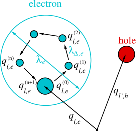
Figure 1: (Color online) Beads representation of electrons and holes. Here $\lambda_{e}^{2}=2\pi\hbar^{2}\beta/m_{e}$, $\lambda_{\Delta,e}^{2}=2\pi\hbar^{2}\epsilon/m_{e}$ and $\sigma=\sigma^{\prime}$. The holes have a similar beads representation. For simplicity bead distribution of holes is not resolved in the figure.

Figure. 1 illustrates the representation of one (light) electron and one (heavy) hole. The circle around the electron beads symbolizes the region that mainly contributes to the path integral partition function. The size of this region is of the order of the thermal electron wavelength $\lambda_{e}$, while typical distances between electron beads are of the order of the electron wavelength taken at an $M$-times higher temperature. The same representation is valid for each hole but it is not shown. In the simulations discussed below the holes are treated according to the full beads representation.

The problem of approximation of factoring the exponential of Hamiltonian $e^{-i\epsilon{\hat{H}}}\approx e^{-i\epsilon{\hat{U}^{c}}}e^{-i\epsilon{\hat{K}}}$ in time-dependent quantum-mechanical methods has been considered in details in Kosloff . For time-dependent problems short-time propagators are described: the second-order differencing and the split operator. The time-independent approaches based on a polynomial expansion of the evolution operator such as the Chebychev propagation and the Lanczos recurrence, have been suggested and considered. These methods as applied to many particle systems result to additional computational problems in comparison with used here simple approximation. Investigation of advantage of methods Kosloff require special work.

III Pair approximation in high-temperature asymptotics for density matrix.

In this section we discuss approximations for the high-temperature density matrix useful for efficient path integral Monte Carlo (PIMC) simulations. It involves the effective exchange pseudopotential allowing for Pauli blocking ( $\tilde{v}^{a}_{lt}$) and pseudopotential of interparticle interaction ($\Phi_{ab}$). Here, we closely follow Huang and earlier work FiBoEbFo01 , where details and further references can be found.

III.1 Exchange effects in pair approximation

To explain the basic ideas of our approach it is enough to consider the system of ideal electrons and holes, so here $\hat{U}\equiv 0$. The hamiltonian of the system (${\hat{H}}={\hat{K}}={\hat{K}_{e}}+{\hat{K}_{h}}$) consists of kinetic energy of electrons ${\hat{K}_{e}}$ and holes ${\hat{K}_{h}}$. Due to the commutativity of these operators the representation of density matrix (3) is exact at any finite number $M$. For our purpose it is enough to consider the sum over permutations in pair approximation at $M=1$:

$$\sum_{\sigma}\sum_{P_{e}}\sum_{P_{h}}(\pm 1)^{\kappa_{P_{e}}+\kappa_{P_{h}}}\,{\cal S}(\sigma,{\hat{P}_{e}}{\hat{P}_{h}}\sigma_{a}^{\prime})\,{\hat{P}_{e}}{\hat{P}_{h}}\rho\,\big{|}_{x^{1}=x^{(0)},\sigma^{\prime}=\sigma}$$

$$=\sum_{\sigma_{e}}\sum_{P_{e}}(\pm 1)^{\kappa_{P_{e}}}{\cal S}(\sigma_{e},{\hat{P}_{e}}\sigma_{e}^{\prime})\,\rho_{e}\big{|}_{x_{e}^{1}=x_{e}^{(0)},\sigma_{e}^{\prime}=\sigma_{e}}\,$$

$$\times\sum_{\sigma_{h}}\sum_{P_{h}}(\pm 1)^{\kappa_{P_{h}}}{\cal S}(\sigma_{h},{\hat{P}_{h}}\sigma_{h}^{\prime})\,\rho_{h}\big{|}_{x_{h}^{1}=x_{h}^{(0)},\sigma_{h}^{\prime}=\sigma_{h}}$$

$$=\sum_{\sigma_{e}}\left\{1-\sum_{l<t}f^{2}_{e;lt}+\sum_{l,t,c}f_{e;lt}f_{e;lc}f_{e;tc}-\dots\right\}$$

$$\times\sum_{\sigma_{h}}\left\{1-\sum_{l<t}f^{2}_{h;lt}+\sum_{l,t,c}f_{h;lt}f_{h;lc}f_{h;tc}-\dots\right\}\approx\,$$

$$\approx\,\sum_{\sigma_{e}}\prod_{l<t}(1-f^{2}_{e;lt})\sum_{\sigma_{h}}\prod_{l<t}(1-f^{2}_{h;lt})=\sum_{\sigma}\exp(-\beta\sum_{l<t}\tilde{v}^{e}_{lt})\exp(-\beta\sum_{l<t}\tilde{v}^{h}_{lt})$$ (4)

where

$$f_{a;lt}=\exp(-\frac{\pi|x^{(0)}_{l,a}-x^{(0)}_{t,a}|^{2}}{\lambda_{a}^{2}}))$$

$$\tilde{v}^{a}_{lt}=-kT\ln(1-f_{a;lt}f_{a;tl})=-kT\ln(1-\delta_{\sigma_{l,a}\sigma_{t,a}}\exp(-\frac{2\pi|x^{(0)}_{l,a}-x^{(0)}_{t,a}|^{2}}{\lambda_{a}^{2}}))$$ (5)

is exchange potential Huang . This formula shows that the first corrections accounting for the antisymmetrization of the density matrix result in the endowing particles by the pair exchange potential $\tilde{v}^{a}_{lt}$. Below to take into account exchange effects in Wigner functions we are going to use analogous pair potential depending on the phase space variables.

III.2 Kelbg potential

High-temperature density matrix $\rho^{(m)}=\langle x^{(m)}|e^{-\epsilon{\hat{H}}}|x^{(m+1)}\rangle$ can be expressed in terms of two-particle density matrices (higher order terms become negligible at sufficiently high temperature $M/\beta$ FiBoEbFo01 ) given by

$$\rho_{ab}(x_{l,a},x^{\prime}_{l,a},x_{t,b},x^{\prime}_{t,b};\beta) = \frac{(m_{a}m_{b})^{3/2}}{(2\pi\hbar\beta)^{3}}\exp\left[-\frac{m_{a}}{2\hbar^{2}\beta}(x_{l,a}-x^{\prime}_{l,a})^{2}\right]\,$$ (6)

$$\times\exp\left[-\frac{m_{b}}{2\hbar^{2}\beta}(x_{t,b}-x^{\prime}_{t,b})^{2}\right]\exp[-\beta\Phi^{OD}_{ab}]\,.$$

This results from factorization of density matrix into kinetic and potential parts, $\rho_{ab}\approx\rho_{0}^{K}\rho^{U}_{ab}$. The off – diagonal density matrix element (6) involves an effective pair interaction which is expressed approximately via its diagonal elements, $\Phi^{OD}_{ab}(x_{l,a},x^{\prime}_{l,a},x_{t,b},x^{\prime}_{t,b};\beta)\approx[\Phi_{ab}(x_{l,a}-x_{t,b};\beta)+\Phi_{ab}(x^{\prime}_{l,a}-x^{\prime}_{t,b};\beta)]/2$, for which we use the well known Kelbg potential Ke63 ; kelbg

$$\Phi_{ab}(x_{lt};\epsilon)=\frac{e_{a}e_{b}}{\lambda_{ab}x_{lt}}\,\left[1-e^{-x_{lt}^{2}}+\sqrt{\pi}x_{lt}\left(1-{\rm erf}(x_{lt})\right)\right],$$ (7)

where $e_{a}$ and $e_{b}$ are charges of particles, $x_{lt}=|x_{l,a}-x_{t,b}|/\lambda_{ab}$, $\lambda_{ab}=\sqrt{\hbar^{2}\epsilon/(2m_{ab})},$ $m_{ab}=m_{a}m_{b}/(m_{a}+m_{b})$ is the reduced mass of the $(ab)$-pair of particles and the error function is defined by ${\rm erf}(x)=\frac{2}{\sqrt{\pi}}\int_{0}^{x}dte^{-t^{2}}$.

Note that the Kelbg potential is finite at zero distance, which is a consequence of allowing for quantum effects. The validity of this potential and its off–diagonal approximation are restricted to temperatures substantially higher than the binding energy afilinov-etal.04pre ; ebeling_sccs05 which puts lower bound on the number of time slices $M$. For discussion of other effective potentials, we refer to FiBoEbFo01 ; afilinov-etal.04pre ; ebeling_sccs05 ; KTR94 .

Summarizing the above approximations, we can conclude that approximations Eqs.(6,7) of each high-temperature factors on the r.h.s. of Eq. (3) carries an error of the order $1/M^{2}$. Within these approximations, we obtain the result

$$\rho^{(m)}=e^{-\epsilon U(x^{(m)},x^{(m+1)})}\rho_{0}^{(m)}+{\cal O}[(1/M)^{2}]$$

where $U$ denotes the sum of all interaction energies, each consisting of the respective sum of pair interactions given by Kelbg potentials, $U(x^{(m)},x^{(m+1)})=(U_{hh}(x_{h}^{(m)})+U_{ee}(x_{e}^{(m)})+U_{eh}(x_{h}^{(m)},x_{e}^{(m)})+U_{hh}(x_{h}^{(m+1)})+U_{ee}(x_{e}^{(m+1)})+U_{eh}(x_{h}^{(m+1)},x_{e}^{(m+1)}))/2$. Product of high temperature matrix elements $\rho^{(m)}$ in Eq. (3) has the total error proportional to $1/M$ and in the limit $M\to\infty$ presents the exact path integral representation of partition function FiBoEbFo01 .

IV Path integral representation of Wigner function

Average value of arbitrary quantum operator $\hat{A}$ can be written as Weyl’s symbol $A(p,x)$ averaged over phase space with the Wigner function $W(p,x;\beta)$ as weight:

$$\langle\hat{A}\rangle=\int\frac{dpdx}{(2\pi\hbar)^{6N}}A(p,x)W(p,x;\beta),$$ (8)

where the Weyl’s symbol of operator $\hat{A}$ is :

$$A(p,x)=\int d\xi e^{-i\langle\xi|p\rangle/\hbar}\langle x-\xi/2|\hat{A}|x+\xi/2\rangle.$$ (9)

Weyl’s symbols for usual operators like $\hat{p}$, $\hat{x}$, $\hat{p}^{2}$, $\hat{x}^{2}$, $\hat{H}$, $\hat{H}^{2}$ etc. can be easily calculated directly from definition (9).

Antisymmetrized Wigner function can be written in the form:

$$W(p,x;\beta)=\frac{1}{Z(\beta)N_{e}!N_{h}!\lambda_{e}^{3N_{e}}\lambda_{h}^{3N_{h}}}\sum_{\sigma}\sum_{P_{e}}\sum_{P_{h}}(\pm 1)^{\kappa_{P_{e}}+\kappa_{P_{h}}}{\cal S}(\sigma,{\hat{P}_{e}}{\hat{P}_{h}}\sigma^{\prime})\big{|}_{\sigma^{\prime}=\sigma}\,$$

$$\times\int d\xi e^{i\langle\xi|p\rangle/\hbar}\langle x-\xi/2|\prod_{m=0}^{M-1}e^{-\epsilon{\hat{U}_{m}^{c}}}e^{-\epsilon{\hat{K}_{m}}}|{\hat{P}_{e}}{\hat{P}_{h}}(x+\xi/2)\rangle\,$$ (10)

Now replacing variables of integration $x^{(m)}$ with $q^{(m)}$ for any given permutation $P_{e}P_{h}$:

$$x_{e}^{(m)}=(P_{e}x_{e}-x_{e})\frac{m}{M}+x_{e}+q^{(m)}_{e}-\frac{(M-m)\xi_{e}}{2M}+\frac{mP_{e}\xi_{e}}{2M}\,$$

$$x_{h}^{(m)}=(P_{h}x_{h}-x_{h})\frac{m}{M}+x_{h}+q^{(m)}_{h}-\frac{(M-m)\xi_{h}}{2M}+\frac{mP_{h}\xi_{h}}{2M}\,$$ (11)

we obtain

$$W(p,x;\beta)=\frac{C(M)}{Z(\beta)N_{e}!N_{h}!\lambda_{e}^{3N_{e}}\lambda_{h}^{3N_{h}}}\sum_{\sigma}\sum_{P_{e}}\sum_{P_{h}}(\pm 1)^{\kappa_{P_{e}}+\kappa_{P_{h}}}{\cal S}(\sigma,{\hat{P}_{e}}{\hat{P}_{h}}\sigma^{\prime})\big{|}_{\sigma^{\prime}=\sigma}\,$$

$$\int d\xi\,\int dq^{(1)}\dots dq^{(M-1)}\exp\Biggl{\{}-\pi\frac{\langle\xi|P_{e}P_{h}+E|\xi\rangle}{2M}+i\langle\xi|p\rangle-\pi\frac{|P_{e}P_{h}x-x|^{2}}{M}$$

$$-\sum\limits_{m=0}^{M-1}\biggl{[}\pi|q^{(m)}-q^{(m+1)}|^{2}+\epsilon U\biggl{(}(P_{e}P_{h}x-x)\frac{m}{M}+x+q^{(m)}-\frac{(M-m)\xi}{2M}+\frac{mP_{e}P_{h}\xi}{2M}\biggr{)}\biggr{]}\Biggr{\}}$$

where $E$ is unit matrix, while matrix presenting permutation $P_{e}P_{h}$ is equal to unit matrix with appropriately transposed columns. Here and further we imply that momentum and coordinate are dimensionless variables like $p_{l,a}\tilde{\lambda}_{a}/\hbar$ and $x_{l,a}/\tilde{\lambda}_{a}$, where $\tilde{\lambda}_{a}=\sqrt{\frac{2\pi\hbar\beta}{m_{a}M}}$. Here constant $C(M)$ as will be shown further is canceled in calculations of average values of operators.

When $\epsilon\to 0$ this multiple integral turns to exact representation of the Wigner function $W(p,x;\beta)$ in the form of path integral with continuous dimensionless ’imaginary time’ $\tau$ feynman-hibbs , which corresponds to $m/M$ in discrete case. Also the set of independent variables $q^{(m)}$ turns into closed trajectory $q(\tau)$. This trajectory starts and ends in $0$ when $\tau=0$ and $1$.

Let us note that integration here relates to the integration over the Wiener measure of all closed trajectories $q(\tau)$. In fact, a particle is presented by the trajectory with characteristic size of order $\lambda_{a}=\sqrt{\frac{2\pi\hbar\beta}{m_{a}}}$ in coordinate space. This is manifestation of the uncertainty principle.

V Harmonic and linear approximation for Wigner function

The expression for Wigner function (IV) is inconvenient for Monte Carlo simulations because it does not contain explicit result of integration over $\xi$ even in case of free particle ($U(x)=0$). In general this integral can not be calculated analytically. Exclusions are the linear or harmonic potentials.

To do this integration analytically and to obtain explicit expression for Wigner function let us take the approximation for potential $U(x)$ arising from the Taylor expansion up to the first or second order in the variables $\xi$:

$$U\biggl{(}(P_{e}P_{h}x-x)\frac{m}{M}+x+q^{(m)}-\frac{(M-m)\xi}{2M}+\frac{mP_{e}P_{h}\xi}{2M}\biggr{)}\approx U\biggl{(}(P_{e}P_{h}x-x)\frac{m}{M}+x+q^{(m)}\biggr{)}$$

$$-\Biggl{\langle}\frac{(M-m)\xi}{2M}-\frac{mP_{e}P_{h}\xi}{2M}\bigg{|}\frac{\partial U((P_{e}P_{h}x-x)\frac{m}{M}+x+q^{(m)})}{\partial x}\Biggr{\rangle}+$$

$$+\frac{1}{2}\Biggl{\langle}\frac{(M-m)\xi}{2M}-\frac{mP_{e}P_{h}\xi}{2M}\bigg{|}\frac{\partial^{2}U((P_{e}P_{h}x-x)\frac{m}{M}+x+q^{(m)})}{\partial x^{2}}\,\bigg{|}\frac{(M-m)\xi}{2M}-\frac{mP_{e}P_{h}\xi}{2M}\Biggr{\rangle}.$$ (13)

Here the second term means scalar product of the vector related to combination of $\xi$ and the multidimensional gradient of pseudopotential, while third term means quadratic form with the matrix of the second derivatives.

This approximation for Wigner function takes the form of gaussian integral and can be calculated analytically. Here for simplicity let us consider expressions related to linear approximation accounting for the linear term in expansion. Accounting for quadratic term is obvious. Then the Wigner function can be written in the following form:

$$W(p,x;\beta)=\frac{C(M)}{Z(\beta)N_{e}!N_{h}!\lambda_{e}^{3N_{e}}\lambda_{h}^{3N_{h}}}\sum_{\sigma}\sum_{P_{e}}\sum_{P_{h}}(\pm 1)^{\kappa_{P_{e}}+\kappa_{P_{h}}}{\cal S}(\sigma,{\hat{P}_{e}}{\hat{P}_{h}}\sigma^{\prime})\big{|}_{\sigma^{\prime}=\sigma}\,$$

$$\times\int dq^{(1)}\dots dq^{(M-1)}\exp\Biggl{\{}-\sum\limits_{m=0}^{M-1}\biggl{[}\pi|q^{(m)}-q^{(m+1)}|^{2}+\epsilon U\biggl{(}(P_{e}P_{h}x-x)\frac{m}{M}+x+q^{(m)}\biggr{)}\biggr{]}\Biggr{\}}$$

$$\times\exp\Biggl{\{}-\pi\frac{|P_{e}P_{h}x-x|^{2}}{M}\Biggr{\}}\int d\xi\,\exp\Biggl{\{}-\pi\frac{\langle\xi|P_{e}P_{h}+E|\xi\rangle}{2M}$$

$$+\Biggl{\langle}\xi\Bigg{|}ip+\sum\limits_{m=0}^{M-1}\bigg{|}\frac{(M-m)}{2M}E-\frac{m}{2M}P_{e}P_{h}\bigg{|}\frac{\partial\epsilon U(\bar{x})}{\partial\bar{x}}\Biggr{\rangle}\Biggr{|}_{\bar{x}=(P_{e}P_{h}x-x)\frac{m}{M}+x+q^{(m)}}\Biggr{\}}.$$ (14)

This expression for Wigner function is obtained under assumption that potential energy $U$ is expandable in Taylor series on $\xi$ with a good accuracy. Let us discuss the legality of such assumption for one particle in 1D case and identical permutation. The Taylor expansion of potential function contains powers of $\xi$ multiplied on $\sum\limits_{m=0}^{M-1}(m/M-1/2)^{n}\frac{\partial^{n}U(x+q_{m})}{n!\partial x^{n}}$. Using mean value theorem, we can roughly get symbolic estimation of these sums as

$$\sum\limits_{m=0}^{M-1}(m/M-1/2)^{n}\frac{\partial^{n}U(x+q^{(m)})}{n!\partial x^{n}}\approx\int\limits_{0}^{1}{d\tau}\frac{1}{n!}\frac{\partial^{n}U(x+q^{(\tau)})}{\partial x^{n}}\left(\tau-\frac{1}{2}\right)^{n}\approx\frac{1}{n!}\frac{(1+(-1)^{n})}{(n+1)2^{n+1}}\frac{\partial^{n}U(x+q^{(0)})}{\partial x^{n}},$$ (15)

where $q^{(0)}=q^{(M)}=0$. We expect the fast convergence of the Taylor series for potentials averaged along the trajectories $x+q^{(m)}$ with sign alternating for odd $n$ weight $\left(\tau-\frac{1}{2}\right)^{n}$. Numerical valuee of this integral rapidly decreases as $1/24$, $1/1920$ and $1/322560$ for $n=2,4,6$ and are lesser for odd $n$. To check the accuracy of this approximation Monte Carlo simulations of the thermodynamic values of particles in different arbitrary potentials have been carried out in LarkinFilinovCPP ; JAMP . These calculations confirm our expectations.

As was mentioned before it is enough for our purpose (see Eq.(4)) to take into account pair permutations. In degenerate system average distance between fermions is less than the thermal wavelength $\lambda$ and trajectories in path integrals (V) are strongly entangled. This is the reason that pair permutations can not strongly affect the potential energy in (V) in comparison with the case of identical permutation. So for any pair permutation the potential energy in (V) can be presented as energy related to identical permutation (of order $N^{2}M/2$) and small (in comparison with identical permutation) difference (of order $2NM$):

$$\sum\limits_{m=0}^{M-1}\epsilon U\biggl{(}(P_{e}P_{h}x-x)\frac{m}{M}+x+q^{(m)}\biggr{)}-\sum\limits_{m=0}^{M-1}\epsilon U\biggl{(}x+q^{(m)}\biggr{)}.$$ (16)

So we can take only the first terms of the perturbation series on this relative difference and can obtain the following simplification: $\sum\limits_{m=0}^{M-1}\epsilon U\biggl{(}(P_{e}P_{h}x-x)\frac{m}{M}+x+q^{(m)}\biggr{)}\approx\sum\limits_{m=0}^{M-1}\epsilon U\biggl{(}x+q^{(m)}\biggr{)}$. Rigorous proof can be done within generalization of Mayer expansion technique (so called algebraic approach) on non ideal systems of particles developed in Zelener ; Ruelle . Now all permutations in (V) are acting only on variables $x$ and $\xi$ and can be beared out of the path integral.

So the Wigner function is determined by path integral over all closed trajectories and can be presented in the form

$$W(p,x;\beta)\approx\,\frac{C(M)}{Z(\beta)N_{e}!N_{h}!\lambda_{e}^{3N_{e}}\lambda_{h}^{3N_{h}}}\int dq^{(1)}\dots dq^{(M-1)}$$

$$\times\exp\Biggl{\{}-\sum\limits_{m=0}^{M-1}\biggl{[}\pi|q^{(m)}-q^{(m+1)}|^{2}+\epsilon U\biggl{(}x+q^{(m)})\biggr{]}\Biggr{\}}$$

$$\times\exp\Biggl{\{}\frac{M}{4\pi}\Biggr{|}ip+\frac{\epsilon}{2}\sum\limits_{m=0}^{M-1}\frac{(M-2m)}{M}\frac{\partial U(x+q^{(m)})}{\partial x}\Biggr{|}^{2}\Biggr{\}}$$

$$\times\sum_{\sigma_{e}}\Biggl{\{}1-\sum_{l<t}\delta_{\sigma_{l,e}\sigma_{t,e}}\exp(-2\pi\frac{|x_{l,e}-x_{t,e}|^{2}}{M})\delta\biggl{(}\frac{(\tilde{p}_{l,e}-\tilde{p}_{t,e})\sqrt{M}}{2\pi}\biggr{)}\Biggr{\}}$$

$$\times\sum_{\sigma_{h}}\Biggl{\{}1-\sum_{l<t}\delta_{\sigma_{l,h}\sigma_{t,h}}\exp(-2\pi\frac{|x_{l,h}-x_{t,h}|^{2}}{M})\delta\biggl{(}\frac{(\tilde{p}_{l,h}-\tilde{p}_{t,h})\sqrt{M}}{2\pi}\biggr{)}\Biggr{\}}$$ (17)

where

$$\tilde{p}_{t,a}=p_{t,a}+\frac{\epsilon}{2}\sum\limits_{m=0}^{M-1}\frac{\partial U(x+q^{(m)})}{\partial x_{t,a}}$$

The main idea of deriving expression (V) can be explained on example of two electrons in $1D$ space. For two electrons the sum over permutations in (V) consists of two terms related to identical permutation (matrix $P$ is equal to unit matrix $E$) and non identical permutation (matrix $P$ is equal to matrix $E$ with transposed columns). To do integration in (V) over $\xi$ let us analyze eigenvalues of matrix $P+E$. For identical permutation the eigenvalues are equal to each other and are equal to two, while the eigenvalues of matrix $P+E$ related to non identical permutation are equal to zero and two. Integration over $\xi$ for identical permutation is trivial, while for non identical permutation matrix $P+E$ have to be presented in the form $P+E=ODO^{-1}$, where $D$ is diagonal matrix with zero and two as the diagonal elements. Here matrix $O$ and inverse matrix $O^{-1}$ are given by the formulas:

$$O=\left|\begin{array}[]{cc}1&1\\ -1&1\\ \end{array}\right|.$$

$$O^{-1}=\frac{1}{2}\left|\begin{array}[]{cc}1&-1\\ 1&1\\ \end{array}\right|.$$

Replacing variables on integration by relation $|\zeta,\eta>=|O^{-1}|\xi>$ one can obtain expression analogous (V).

To obtain the final expression we have to approximate delta-function by the standard Gaussian exponent with small parameter $\alpha$ :

$$W(p,x;\beta)\approx\,\frac{C(M)}{Z(\beta)N_{e}!N_{h}!\lambda_{e}^{3N_{e}}\lambda_{h}^{3N_{h}}}\int dq^{(1)}\dots dq^{(M-1)}$$

$$\times\exp\Biggl{\{}-\sum\limits_{m=0}^{M-1}\biggl{[}\pi|q^{(m)}-q^{(m+1)}|^{2}+\epsilon U(x+q^{(m)})\biggr{]}\Biggr{\}}$$

$$\times\exp\Biggl{\{}\frac{M}{4\pi}\Biggr{|}ip+\frac{\epsilon}{2}\sum\limits_{m=0}^{M-1}\frac{(M-2m)}{M}\frac{\partial U(x+q^{(m)})}{\partial x}\Biggr{|}^{2}\Biggr{\}}\sum_{\sigma}\exp(-\beta\sum_{l<t}v^{e}_{lt})\exp(-\beta\sum_{l<t}v^{h}_{lt})\Biggr{|}^{2}\Biggr{\}}$$

where

$$v^{a}_{lt}=-kT\ln\Biggl{\{}1-\delta_{\sigma_{l,a}\sigma_{t,a}}\exp\biggl{(}-\frac{2\pi|x_{l,a}-x_{t,a}|^{2}}{M}\biggr{)}\frac{\sqrt{M}}{2\pi\alpha}\exp\biggl{(}-\pi\frac{|(\tilde{p}_{l,a}-\tilde{p}_{t,a})\sqrt{M}|^{2}}{(2\pi\alpha)^{2}}\biggr{)}\Biggr{\}}$$

(For functions $v^{a}_{lt}$ we can imply here analytic continuation on complex plane.) Note that the expression (V) contains term related the classical Maxwell distribution explicitly. The difference is in the other terms accounting for influence of interaction on the momentum distribution function. To regularize integration over momenta in the limit of small $\alpha$ it is necessary to rescale $p$ by factor $\frac{\sqrt{M}}{2\pi\alpha}$ in (8), so one can use the simplified version of effective pair exchange pseudopotential ($\pi$ is included in small $\alpha^{2}$):

$$v^{a}_{lt}\approx\,-kT\ln\Biggl{\{}1-\delta_{\sigma_{l,a}\sigma_{t,a}}\exp\biggl{(}-\frac{2\pi|x_{l,a}-x_{t,a}|^{2}}{\lambda^{2}_{a}}\biggr{)}\exp\biggl{(}-\frac{|(\tilde{p}_{l,a}-\tilde{p}_{t,a})\lambda_{a}|^{2}}{(2\pi\hbar)^{2}\alpha^{2}}\biggr{)}\Biggr{\}}$$

Here momenta and coordinates are written in natural units ($\lambda_{a}^{2}=\frac{2\pi\hbar^{2}\beta}{m_{a}}$).

VI Average values of quantum operators

To calculate average values of quantum operators $\langle\hat{A}\rangle$ we are going to use the Monte Carlo method (MC) Metropolis ; Hasting . For this aim we have to use path integrals (V) in discrete form. As a result we obtain final expressions for MC calculations as follows:

$$\langle\hat{A}\rangle=\frac{\left\langle A(p,x)\cdot h(p,x,q^{(1)},\dots,q^{(M-1)})\right\rangle_{w}}{\langle h(p,x,q^{(1)},\dots,q^{(M-1)})\rangle_{w}}.$$ (19)

Here brackets $\bigl{\langle}g(p,x,q^{(1)},\dots,q^{(M-1)})\bigr{\rangle}_{w}$ denote averaging of any function $g(p,x,q^{(1)},\dots,q^{(M-1)})$ with positive weight $w(p,x,q^{(1)},\dots,q^{(M-1)})$:

$$\langle g(p,x,q^{(1)},\dots,q^{(M-1)})\rangle_{w}=\int{dpdx}\int{dq^{(1)}\dots dq^{(M-1)}}g(p,x,q^{(1)},\dots,q^{(M-1)})w(p,x,q^{(1)},\dots,q^{(M-1)})$$ (20)

while

$$w(p,x,q^{(1)},\dots,q^{(M-1)})=\Biggr{|}\cos\Biggr{\{}2\frac{M}{4\pi}\Biggl{\langle}p\Bigg{|}\frac{\epsilon}{2}\sum\limits_{m=0}^{M-1}\frac{(M-2m)}{M}\frac{\partial U(x+q^{(m)})}{\partial x}\Biggr{\rangle}\Biggr{\}}\Biggl{|}$$

$$\times\exp\Biggl{\{}-\frac{M}{4\pi}\biggl{(}\Bigg{|}p\Bigg{|}^{2}+\Bigg{|}\frac{\epsilon}{2}\sum\limits_{m=0}^{M-1}\frac{(M-2m)}{M}\frac{\partial U(x+q^{(m)})}{\partial x}\Biggr{|}^{2}\biggr{)}\Biggr{\}}$$

$$\times\exp\Biggl{\{}-\sum\limits_{m=0}^{M-1}\biggl{[}\pi|q^{(m)}-q^{(m+1)}|^{2}+\epsilon U(x+q^{(m)})\biggr{]}\Biggr{\}}\sum_{\sigma}\exp(-\beta\sum_{l<t}v^{e}_{lt})\exp(-\beta\sum_{l<t}v^{h}_{lt}),$$

$$h(p,x,q^{(1)},\dots,q^{(M-1)})=sign\Biggr{(}\cos\Biggr{\{}2\frac{M}{4\pi}\Biggl{\langle}p\Bigg{|}\frac{\epsilon}{2}\sum\limits_{m=0}^{M-1}\frac{(M-2m)}{M}\frac{\partial U(x+q^{(m)})}{\partial x}\Biggr{\rangle}\Biggr{\}}\Biggl{)}.$$ (21)

Note that denominator in (19) is equal to nominator with $A(p,x)=1$, so $C(M)$ from (V) is canceled.

Eq. (19) can be rewritten in compact form:

$$\langle A\rangle_{w}=\frac{\sum_{i=1}^{N}A(p_{i},x_{i})h(\overline{\mathbf{x}}_{i})}{\sum_{i=1}^{N}h(\overline{\mathbf{x}}_{i})}.$$ (22)

where $h(\overline{\mathbf{x}}_{i})$ is arbitrary weight function of the random quantity $\overline{\mathbf{x}}_{i}$ drawn from any distribution $w(\overline{\mathbf{x}})/\overline{Q}$  ($\overline{Q}=\int_{\Omega}w(\overline{\mathbf{x}})d\overline{\mathbf{x}}).$

Metropolis – Hastings algorithm resides in designing a Markov process (by constructing transition probabilities $P(\overline{\mathbf{x}}\rightarrow\overline{\mathbf{x}}^{\prime})$ ), such that its stationary distribution to be equal to $w(\overline{\mathbf{x}})$. The derivation of the algorithm starts with the condition of detailed balance:

$$w(\overline{\mathbf{x}})P(\overline{\mathbf{x}}\rightarrow\overline{\mathbf{x}}^{\prime})=w(\overline{\mathbf{x}}^{\prime})P(\overline{\mathbf{x}}^{\prime}\rightarrow\overline{\mathbf{x}})$$ (23)

which can be rewritten as

$$\frac{P(\overline{\mathbf{x}}\rightarrow\overline{\mathbf{x}}^{\prime})}{P(\overline{\mathbf{x}}^{\prime}\rightarrow\overline{\mathbf{x}})}=\frac{w(\overline{\mathbf{x}}^{\prime})}{w(\overline{\mathbf{x}})}.$$ (24)

The idea is to separate the transition in two sub-steps: the proposal and the acceptance-rejection. The transition probability can be written as the product: $P(\overline{\mathbf{x}}\rightarrow\overline{\mathbf{x}}^{\prime})=g(\overline{\mathbf{x}}\rightarrow\overline{\mathbf{x}}^{\prime})A(\overline{\mathbf{x}}\rightarrow\overline{\mathbf{x}}^{\prime})$. The proposal distribution $\displaystyle g(\overline{\mathbf{x}}\rightarrow\overline{\mathbf{x}}^{\prime})$ is the conditional probability of proposing a state $\overline{\mathbf{x}}^{\prime}$ for given $\overline{\mathbf{x}}$, and the acceptance distribution $\displaystyle A(x\rightarrow x^{\prime})$ is the conditional probability to accept the proposed state $\overline{\mathbf{x}}^{\prime}$. Inserting this relation in the previous equation, we have

$$\frac{A(\overline{\mathbf{x}}\rightarrow\overline{\mathbf{x}}^{\prime})}{A(\overline{\mathbf{x}}^{\prime}\rightarrow\overline{\mathbf{x}})}=\frac{w(\overline{\mathbf{x}}^{\prime})}{w(\overline{\mathbf{x}})}\frac{g(\overline{\mathbf{x}}^{\prime}\rightarrow\overline{\mathbf{x}})}{g(\overline{\mathbf{x}}\rightarrow\overline{\mathbf{x}}^{\prime})}$$ (25)

.

Then it is necessary to choose an acceptance that fulfills detailed balance. One common choice is the Metropolis’s suggestion:

$$A(\overline{\mathbf{x}}\rightarrow\overline{\mathbf{x}}^{\prime})=\min\left(1,\frac{w(\overline{\mathbf{x}}^{\prime})}{w(\overline{\mathbf{x}})}\frac{g(\overline{\mathbf{x}}^{\prime}\rightarrow\overline{\mathbf{x}})}{g(\overline{\mathbf{x}}\rightarrow\overline{\mathbf{x}}^{\prime})}\right)$$ (26)

This means that we always accept when the acceptance is bigger than 1 and we can accept or reject when the acceptance is smaller than 1. As the conditional probability $g$ we can use

$$g(\overline{\mathbf{x}}\rightarrow\overline{\mathbf{x}}^{\prime})=\exp\Biggl{\{}-\frac{M}{4\pi}\biggl{(}\Bigg{|}p^{\prime}\Bigg{|}^{2}+\Bigg{|}\frac{\epsilon}{2}\sum\limits_{m=0}^{M-1}\frac{(M-2m)}{M}\frac{\partial U(x^{\prime}+q^{(m)})}{\partial x^{\prime}}\Biggr{|}^{2}\biggr{)}\Biggr{\}}/$$ (27)

$$\exp\Biggl{\{}-\frac{M}{4\pi}\biggl{(}\Bigg{|}p\Bigg{|}^{2}+\Bigg{|}\frac{\epsilon}{2}\sum\limits_{m=0}^{M-1}\frac{(M-2m)}{M}\frac{\partial U(x+q^{(m)})}{\partial x}\Biggr{|}^{2}\biggr{)}\Biggr{\}}$$ (28)

.

The Metropolis – Hastings algorithm can consist in the following:
1) Initialization: pick an initial state point $(p,x,q^{(1)},\dots,q^{(M-1)})=\overline{\mathbf{x}}$ at random;
2) randomly pick a state $x^{\prime}$ according to $\displaystyle g(\overline{\mathbf{x}}\rightarrow\overline{\mathbf{x}}^{\prime})$;
3) accept the state according to the probability $\displaystyle A(\overline{\mathbf{x}}\rightarrow\overline{\mathbf{x}}^{\prime})$. If not accepted, that means that $\overline{\mathbf{x}}^{\prime}=\overline{\mathbf{x}}$, and so there is no need to update anything. Else, the system transits to $\overline{\mathbf{x}}^{\prime}$;
4) go to 2 until many $M$ states were generated;
5) save the state $\overline{\mathbf{x}}$, go to $2$.

It is important to notice that it is not clear, in a general problem, which distribution $\displaystyle g(\overline{\mathbf{x}}\rightarrow\overline{\mathbf{x}}^{\prime})$ one should use. It is a free parameter of the method which has to be adjusted to the particular problem ’in hand’. This is usually done by calculating the acceptance rate, which is the fraction of proposed samples that is accepted during the last $\displaystyle N$ samples. As has been shown theoretically the ideal acceptance rate have to be in interval of $23$ – $50$ %. The Markov chain is started from an arbitrary initial value $\displaystyle\overline{\mathbf{x}}_{0}$ and the algorithm is run for many iterations until this initial state is "forgotten". These samples, which are discarded, are known as ’burn-in’. The remaining set of accepted values of $\overline{\mathbf{x}}$ represent a sample from the distribution $w(\overline{\mathbf{x}})$.

To construct Metropolis – Hasting algorithm Metropolis ; Hasting we introduce three types of PIMC steps:

1. Variation of momentum of some particle.

2. Variation of overall position of some particle.

3. Variation of trajectory representing some particle.

The first thousands of steps should be rejected during the calculation to "forget" initial configuration. Periodic boundary conditions have to be used to reduce finite number effects Metropolis .

Calculations of the average values of quantum operators depending only on coordinates of particles is more convenient and reasonable to carry out in configurational space by standard path integral Monte Karlo method (PIMC). Within considered above approach it can be done if we change the following functions:

$$\tilde{w}(x,q^{(1)},\dots,q^{(M-1)})=\exp\Biggl{\{}-\sum\limits_{m=0}^{M-1}\biggl{[}\pi|q^{(m)}-q^{(m+1)}|^{2}+\epsilon U(x+q^{(m)})\biggr{]}\Biggr{\}}\sum_{\sigma}\exp(-\beta\sum_{l<t}\tilde{v}^{e}_{lt})\exp(-\beta\sum_{l<t}\tilde{v}^{h}_{lt}),$$

$$\tilde{h}(x,q^{(1)},\dots,q^{(M-1)})\equiv 1.$$ (29)

where $\tilde{v}^{a}_{lt}$ is defined by equation (5),

$$\langle g(x,q^{(1)},\dots,q^{(M-1)})\rangle_{\tilde{w}}=\int{dx}\int{dq^{(1)}\dots dq^{(M-1)}}g(x,q^{(1)},\dots,q^{(M-1)})\tilde{w}(x,q^{(1)},\dots,q^{(M-1)})$$ (30)

and

$$\langle{\tilde{\hat{A}}}\rangle=\frac{\left\langle\tilde{A}(x)\cdot\tilde{h}(x,q^{(1)},\dots,q^{(M-1)})\right\rangle_{\tilde{w}}}{\langle\tilde{h}(x,q^{(1)},\dots,q^{(M-1)})\rangle_{\tilde{w}}}.$$ (31)

VII Results of numerical calculations

We define momentum distribution functions and pair correlation functions for holes ($a=h$) and electrons ($a=e$) by the following expressions:

$$w_{a}(|p|)=\frac{\left\langle\delta(|p_{1,a}|-|p|)\cdot h(p,x,q^{(1)},\dots,q^{(M-1)})\right\rangle_{w}}{\langle h(p,x,q^{(1)},\dots,q^{(M-1)})\rangle_{w}}$$

$$g_{ab}(r)=\frac{\left\langle\delta(|x_{1,a}-x_{1,b}|-r)\cdot\tilde{h}(x,q^{(1)},\dots,q^{(M-1)})\right\rangle_{\tilde{w}}}{\langle\tilde{h}(x,q^{(1)},\dots,q^{(M-1)})\rangle_{\tilde{w}}}$$ (32)

where $\delta$ is delta function, $a$ and $b$ are types of the particles. The pair correlation functions $g_{ab}$ give a probability density to find a pair of particles of types $a$ and $b$ at a certain distance $r$ from each other and depend only on the difference of coordinates due to the translational invariance of the system. In a noninteracting classical system, $g_{ab}\equiv 1$, whereas interactions and quantum statistics result in a spatial redistribution of the particles.

The momentum distribution function $w_{a}(|p|)$ gives a probability density for particle of type $a$ to have momentum $p$. Non ideal classical systems of particles due to the commutativity of kinetic and potential energy operators have Maxwell distribution function (MD) proportional to $\exp(-(p\lambda_{a})^{2}/4\pi\hbar^{2})$ even at strong coupling. Quantum effects can affect the shape of kinetic energy distribution function. Quantum ideal systems of particles due to the quantum statistics have Fermi or Bose momentum distribution functions. Interaction of a quantum particle with its surroundings restricts the volume of configuration space, which, can also affect the shape of momentum distribution function due to the uncertainty relation. In this section we present results for both ideal and strongly coupled electron – hole plasmas with different hole masses.

Test calculations for ideal electron – hole plasma. To extent the region of applicability of pair approximation the small parameter $\alpha^{2}$ in Eq. (V) has been used as adjustable function of the universal degeneracy parameter of ideal fermions $n\lambda^{3}$, namely $\alpha^{2}_{a}=0.00505+0.056n\lambda_{a}^{3}$. To simplify calculations we fix the number of electrons and holes with the same spin projection equal to $N_{e}/2$ and $N_{h}/2$ respectively. To test the developed approach calculations of the path integral representation of Wigner function in the form (19) have been carried out for different number of particles and beads presenting each particles. Results have been obtained by averaging-out over several hundred thousands and several millions Monte Carlo steps. It turn out that for convergence is enough several hundred thousand Monte Carlo steps and two hundred particles each presented by twenty beads.

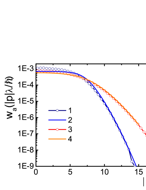
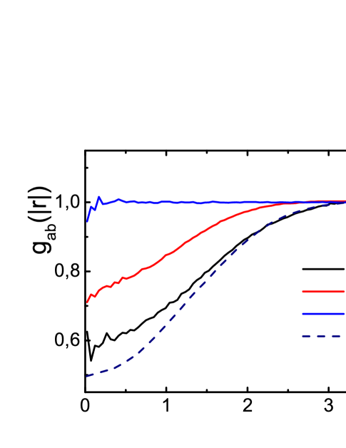
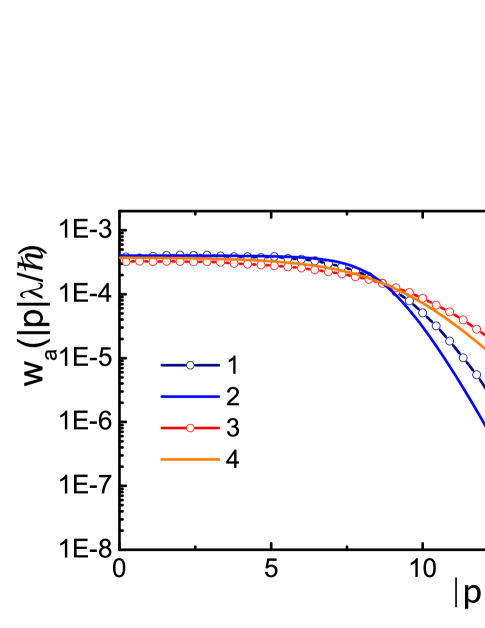
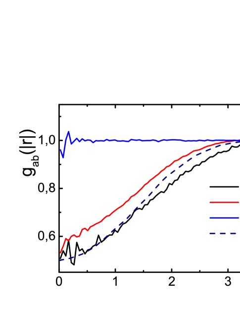
Figure 2: (Color online) The momentum distribution functions $w_{a}(|p|)$ (left panels) and pair correlation functions $g_{ab}(|r|),(a,b=e,h)$ (right panels) for ideal electron - hole plasma at $r_{s}=2$. Left panels: lines $1,3$ show PIMC distributions $w_{a}(|p|)$ scaled by ratio of Plank constant to the electron thermal wavelength ($\frac{\hbar}{\lambda_{e}}$), while lines $2,4$ demonstrate the ideal Fermi distributions for electrons and two times heavier holes respectively; Right panels: lines $1,2,3$ present PIMC electron – electron, hole – hole and electron – hole correlation functions scaled by Bohr radius respectively, while line 4 show results of analytical approximations Bosse for electrons.

Let us start from consideration of ideal fermions. For ideal electron – hole plasma Figure 2 shows the momentum distributions $w_{a}(|p_{a}|),(a=e,h)$ and pair correlation functions $g_{ab}(|r|),(a,b=e,h)$ for electron parameters of degeneracy equal to $n\lambda_{e}^{3}=5.6\,(T/E_{F}=0.208,\,k_{F}\lambda_{e}=5.5)$ and $n\lambda_{e}^{3}=10\,(T/E_{F}=0.141,\,k_{F}\lambda_{e}=6.66)$ for upper to bottom rows respectively. Let us note that holes is this calculations are two times heavier than electrons, so the related parameters of degeneracy is $2^{3/2}$ times smaller. Presented momentum distribution functions are normalized to one. As it follows from the analysis of figure 2 agreement between PIMC calculations and analytical Fermi distributions (FD) is good enough up to parameter of electron degeneracy equal to $n\lambda_{e}^{3}=10\,(T/E_{F}=0.141)$. Here integral characteristics such as energy resulting from PIMC and analytical distribution functions are practically equal to each other.

In the right panels we compare with good agreement the calculated here pair correlation functions with analogous analytical approximations obtained in Bosse for electrons. At the distances lesser than thermal wave length of electron or hole the influence of Fermi repulsion is evident with increasing parameter of degeneracy from upper to bottom rows. At the same time the electron - hole pair correlation functions are identically equal to unit because exchange interaction between particle of different type is missing.

Presented results for momentum distribution functions have been obtained in pair exchange approximation described by effective pair pseudopotentials (V). Figure 3 presents contour panels of exchange pair pseudopotentials for parameter of degeneracy equal to $5.6\,(T/E_{F}=0.208)$. Momenta and coordinates axises are scaled by the electron thermal wave length with Plank constant and factor ten for momentum. As before holes are two times heavier than electrons. As it follows from analysis of Figure 2 the Pauli blocking in phase space accounted for by these exchange pseudopotentials provides agreement of PIMC calculations and analytical FD in wide ranges of fermion degeneracy and fermion momenta, where decay of the distribution functions is at least of five orders of magnitude. It necessary to stress that one of the reason of increasing discrepancy with degeneracy growth is limitation on available computing power allowing calculations with several hundred particles each presented by twenty beads. When parameter of degeneracy is more than $10\,(T/E_{F}=0.141)$ the thermal electron wave length is of order of Monte Carlo cell size and influence of finite number of particles and periodic boundary conditions becomes significant as has been tested in our calculations.

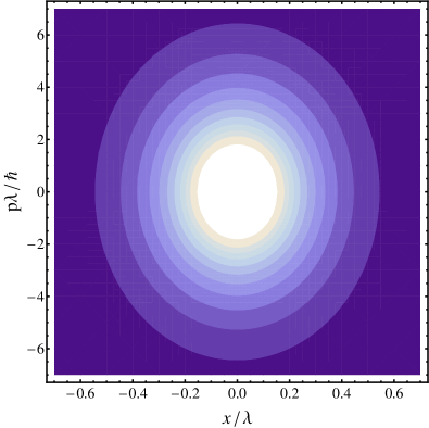
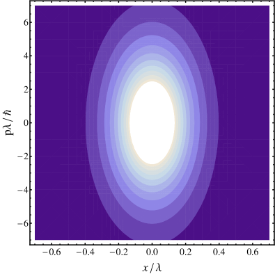
Figure 3: (Color online) Contour plots of the repulsive effective exchange pair pseudopotentials in phase space. Left panel: $m_{e}=1$, dark area $\beta v^{e}_{lt}\approx 0$, white area $\beta v^{e}_{lt}\geq 1.9$. Right panel: $m_{h}=2$, dark area $\beta v^{h}_{lt}\approx 0$, white area $\beta v^{h}_{lt}\geq 1.5$.

Let us stress that detailed test calculation for interacting particle carried out within developed approach in LarkinFilinovCPP ; JAMP have demonstrated good agreement with results of independent calculations by standard path integral Monte Carlo method and available analytical results.

Quantum ’tails’ in the momentum distribution functions. In classical statistics the commutativity of kinetic and potential energy operators leads to the Maxwell distribution (MD) functions even for the strong interparticle interaction. On the contrary for quantum systems the interparticle interaction can affect the maxwellian shape of the particle kinetic energy distribution function, because the interaction of a particle with its surroundings restricts the volume of configuration space and results in an increase in the volume of the momentum space due to the uncertainty principle, i.e., in a rise in the fraction of particles with higher momenta. On other hand Fermi statistical effects accounted by Pauli blocking of fermions can be also important at the same conditions. On account of these effects the momentum distribution functions may contain a power-law tails even under conditions of thermodynamic equilibrium Galitskii ; Kimball ; StarPhys ; Eletskii ; Emelianov ; Kochetov ; StMax .

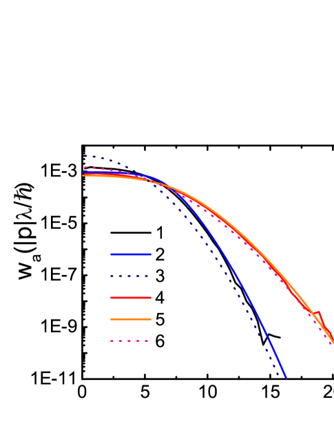
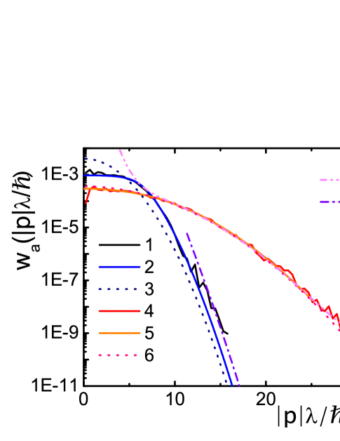
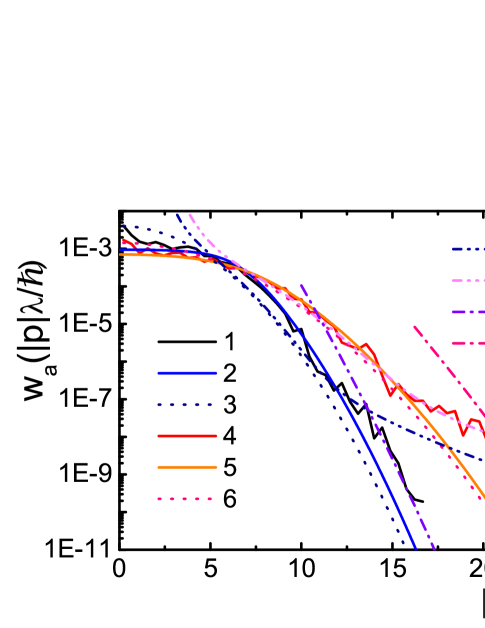
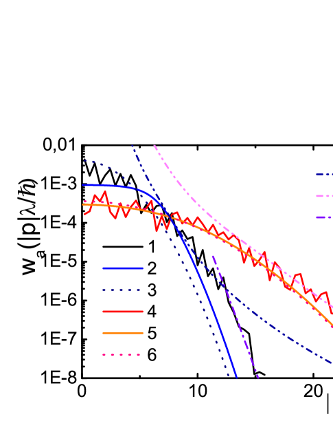
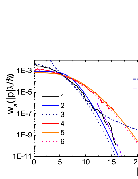
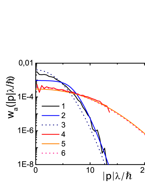
Figure 4: (Color online) The momentum distribution functions $w_{a}(|p|)$ for non - ideal electron – hole plasma. Results for electrons and two (five) times heavier holes are presented by left (right) panels respectively. Electronic momentum distributions are presented by lines (1,2,3,7,9), while analogous results for holes are presented by lines (4,5,6,8,10). Detailed description of the meaning of these lines is given in text. Degeneracy of electrons is equal to 4 ($T/E_{F}=0.261,\,k_{F}\lambda_{e}=4.91$), while $r_{s}$ and plasma classical coupling parameter is equal 1, 2, 4 from upper to bottom rows respectively. Oscillations of PIMC distribution functions designate statistical errors.

In these papers in frameworks of some models and perturbation theories it was shown that for some system of non-relativistic particles the momentum distribution in the asymptotic region of large momenta $p$ may be described by the sum of MD and quantum correction proportional to $const/p^{8}$ (we use short notation as P8) or MD with added product of $const/p^{8}$ and Maxwell distributions with effective temperature that exceeds the temperature of medium (short notation – P8MDEF) StMax . Reliable calculation of numerical parameters in these asymptotic is problematic.

PIMC calculations for the electron and hole momentum distribution functions in electron – hole plasma are presented on Figure 4 by lines 1 and 4 for electrons and holes respectively. Here parameter of electronic degeneracy is equal to four ($T/E_{F}=0.261$) and hole masses in two (left panels) and five (right panels) times larger than electron mass. Figure 4 presents also several related analytical dependencies: FD (lines 2 and 5), MD (lines 3 and 6), P8 (lines 7 and 8), P8MDEF (lines 9 and 10).

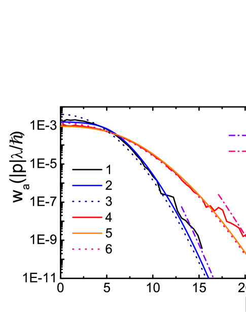
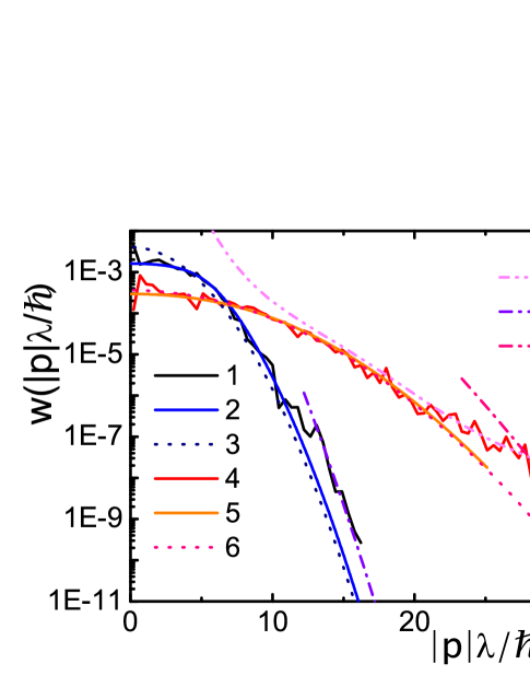
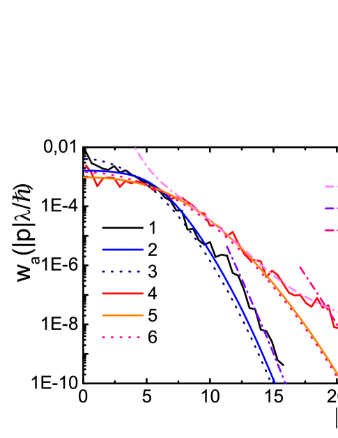
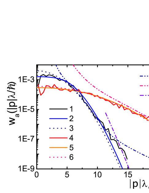
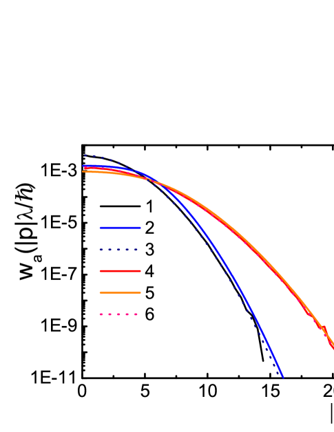
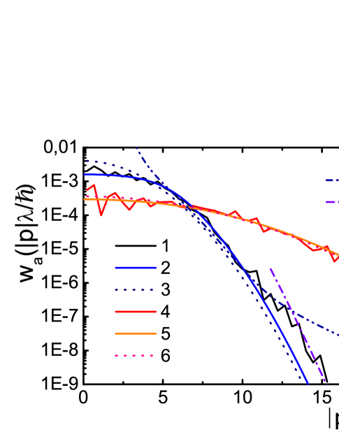
Figure 5: (Color online)The momentum distribution functions $w_{a}(|p|)$ for non - ideal electron – hole plasma. Results for electrons and two (five) times heavier holes are presented by left (right) panels respectively. Electronic momentum distributions are presented by lines (1,2,3,7), while results for holes are presented by lines (4,5,6,8,9). Detailed description of the meaning of these lines is given in text. Degeneracy of electrons is equal to 2 ($T/E_{F}=0.413,\,k_{F}\lambda_{e}=3.9$), while $r_{s}=2,\,3,\,4$ and plasma classical coupling parameter is equal 1.3, 2, 2.6 from upper to bottom rows. Oscillations of PIMC distribution functions designate statistical errors.

Here constant in P8 and effective temperature in P8MDEF have been used as adjustable parameters to fit PIMC momentum distribution functions in large momentum asymptotic regions. All MD and FD are normalized to one. As it follows from analysis of Figure 4 dependence P8 may reliably fit PIMC distributions in intermidiate region between FD and P8MDEF, while the P8MDEF fits PIMC at large momenta on almost all panels of Figure 4.

It is necessary to stress that each type of asymptotics fits PIMC momentum distribution function throughout decaying region of two or even more order of magnitude. Interesting is the non monotonic behavior of discrepancy between PIMC momentum distributions and FD or MD in asymptotic regions with increasing classical coupling parameter $\Gamma=\beta e^{2}/(3/4\pi n_{a})^{1/3}$ from top ($\Gamma=1$) to bottom ($\Gamma=4$) panels. Namely for electrons and holes at low $\Gamma\approx 1$ and high enough $\Gamma\approx 4$ the PIMC distributions are approaching the FD or MD better than at $\Gamma\approx 2$ or $\Gamma\approx 3$.

Physical meaning of this phenomenon is the following. At small $\Gamma\leq 1$ the influence of interparticle interaction is negligible and PIMC momentum distribution functions due to the exchange pseudopotentials ($v^{a}_{lt}\approx 2$) approximate related Fermi distributions. At large $\Gamma\geq 4$ average interparticle interaction is more important than weaker exchange interaction and PIMC momentum distributions are approaching MD, which are very close to FD at large momenta. This means that appearance of quantum ’tails’ in intermediate region of $\Gamma\approx 2,3$ may be explained by simultaneous influence of Coulomb and interparticle exchange interactions.

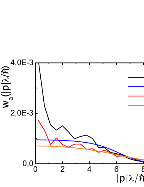
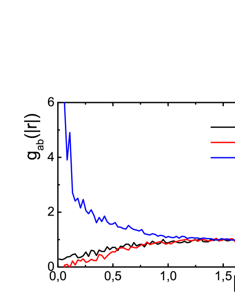
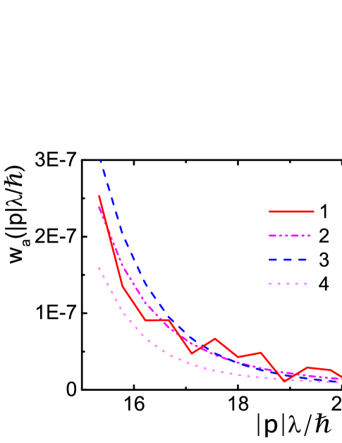
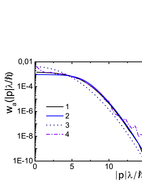
Figure 6: (Color online) Momentum distributions and pair correlation functions for electrons and two times heavier hole at degeneracy of electrons equal to 4 ($T/E_{F}=0.261,\,k_{F}\lambda_{e}=4.91$).
Top left panel: $w_{a}(|p|)$ at $p\lambda/\hbar\leq 10$ and $r_{s}=2$. Lines: 1,2 – PIMC and FD for electrons; 3,4 – PIMC and FD for holes respectively.
Top right panel: $g_{ab}(|r|),(a,b=e,h)$ at $r_{s}=1$ . Lines 1,2,3 present electron - electron, hole - hole and electron - hole distribution functions respectively. Plasma classical coupling parameter is equal $1$. Small oscillations of PIMC distribution functions designate statistical error.
Bottom left panel: power-low approximations $const/p^{n}$ (P8) of PIMC momentum distribution in intermediate region at $r_{s}=2$. Lines: 1 – PIMC momentum distribution; 2 – $const/p^{n}$ for $n=8$; 3 – $const/p^{n}$ for $n=11$; 4 – $const/p^{n}$ for $n=8$.
Bottom right panel: Lines: 1 – PIMC for UEG; 2 – FD; 3 – MD; 4 – PIMC for electron – hole plasma. Classical coupling parameter $\Gamma$ equal to two, $r_{s}=2$

Figure 5 shows PIMC distribution functions for parameter of electronic degeneracy equal to two ($T/E_{F}=0.413$) and $m_{h}=2$ (left panels) and $m_{h}=5$ (right panels). Presented results confirm even more clearly the basic features of asymptotic behavior of PIMC distribution functions discussed above.

Figure 6 presents PIMC momentum distributions and pair correlation functions. At the top left panel at momenta ($p\lambda/\hbar\leq 10$) the PIMC distributions show systematic oscillations and exceeding of FD for both electrons and holes, which is consequence of interparticle interaction resulting in partial ordering of electrons and holes as can be seen from right panel. Typical particle configurations are described by the pair correlation functions presented by the top right panel. This panel shows results of calculation of pair correlation functions for non ideal electron – hole plasma at $\Gamma=1$. On the contrary to ideal plasma the electron – hole pair correlation function increases at the small interparticle distance due to the Coulomb attraction, while electron - electron and hole - hole pair correlation function decreases due to the Coulomb and Fermi repulsion. Coulomb electron - electron repulsion is lesser pronounced in comparison with hole – hole repulsion due to tunneling effects, which are larger for lighter electrons. Here the electron - electron Fermi repulsion is lesser pronounced in comparison with ideal plasma, because the coupling parameter is strong enough (compare this function with related $g_{ee}$ on Figure 2).

Bottom left panel of Figure 6 presents approximation of PIMC momentum distribution function in intermediate region by several power – low dependences with different values of power. Analysis of figure 6 clearly shows validity of approximation described by dependence P8.

To stress the role of interparticle interaction and correlation effects we have carried out calculations of electron momentum distribution functions for the model of uniform electronic gas (UEG) being the quantum mechanical model of interacting electrons where the positive charges are assumed to be uniformly distributed in space. Momentum distribution functions for UEG model and electron – hole plasma are presented by bottom right panel of Figure 6 for parameter of degeneracy equal to four ($T/E_{F}=0.261$), $r_{s}=2$ and classical coupling parameter equal to 2. (the same as for Figure. 4). Comparison of obtained results demonstrates disappearance of quantum ’tail’ and very good agreement of electron momentum distribution functions of UEG with Fermi distribution. Let us stress that studies of momentum distribution functions of UEG by developed approach are at present in progress, while studies of thermodynamic properties of UEG by PIMC and detailed comparison with available data (see for example UEG1 ) have been recently published by the authors of this paper in UEG .

VIII Conclusion

In our work we have derived the new path integral representation of Wigner function of the Coulomb system of particles for canonical ensemble. We have obtained explicit expression of Wigner function in linear approximation resembling the Maxwell – Boltzmann distribution on momentum variables, but with quantum corrections. This approximation contains also the oscillatory multiplier describing quantum interference. We have developed new quantum Monte-Carlo method for calculations of average values of arbitrary quantum operators depending both on coordinates and momenta. PIMC calculations of the momentum distribution function and pair correlation functions for non-ideal plasma have been done. Comparison with classical Maxwell – Boltzmann and quantum Fermi distribution shows the significant influence of the interparticle interaction on the high energy asymptotics of the momentum distribution functions resulting in appearance of quantum ’tails’.

IX Acknowledgements

We acknowledge stimulating discussions with Profs. A.N. Starostin, Yu.V. Petrushevich, W. Ebeling, M. Bonitz, E.E. Son, I.L. Iosilevskii and V.I. Man’ko.

References

- (1) Feynman R P and Hibbs A R 1965 Quantum mechanics and path integrals (New York:McGraw-Hill)
- (2) Wiener N 1923 J. Math. Phys. 2 131
- (3) Galitskii V M and Yakimets V V 1966 Zh. Eksp. Teor. Fiz. 51 957; 1967 Sov. Phys. JETP 24 637
- (4) Kimball J C 1975 J. Phys. A : Math. Gen. 8 No 9 1513
- (5) Starostin A N, Mironov A B, Aleksandrov N L, Fisch N J, Kulsrud R M 2002 Physica A 305 287
- (6) Eletskii A V, Starostin A N and Taran M D 2005 Physics - Uspekhi 48 281
- (7) Emelianov A V, Eremin A V, Petrushevich Yu V, Sivkova E E, Starostin A N, Taran M D, Fortov V E 2011 JETP Letters 94:7 530
- (8) Kochetov I V, Napartovich A P, Petrushevich Yu V, Starostin A N, Taran M D 2016 High Temperature 54:4 563
- (9) Starostin A N, Petrushevich Yu V 2016 Abstracts of Scientific-Coordination Workshop on Non-Ideal Plasma Physics December 7-8, 2016, Moscow, Russia, http://www.ihed.ras.ru/npp2016/program/
- (10) Schoof T, Bonitz M, Filinov A, Hochstuhl D, Dufty J W 2011 Contrib. Plasma Phys. 51 687
- (11) Schoof T, Groth S, Vorberger J and Bonitz M 2015 Phys. Rev. Lett. 115 130402
- (12) Dornheim T, Groth S, Filinov A and Bonitz M. 2015 New J. Phys. 17 073017
- (13) Dornheim T, Groth S, Sjostrom T, Malone F D, Foulkes W M C and Bonitz M 2016 Phys. Rev. Lett. 117 156403
- (14) Wigner E P 1932 Phys. Rev. 40 749
- (15) Tatarskii V 1983 Sov. Phys. Uspekhi 26 311
- (16) W. Ebeling, F. Schautz, Phys. Rev. E, 56, 3498 (1997)
- (17) A.S. Larkin, V.S. Filinov, V.E. Fortov, 2016 Contrib. Plasma Phys. 56 187; arXiv:1703.04448 [physics.plasm-ph]; arXiv:1702.04091 [physics.plasm-ph]
- (18) A.S. Larkin, V.S. Filinov, 2017 Journal of Applied Mathematics and Physics, 5, 392-411
- (19) Zamalin V M and Norman G E 1973 USSR Comp. Math. and Math. Phys. 13 169
- (20) V. M. Zamalin, G. E. Norman, and V. S. Filinov, 1977 The Monte-Carlo Method in Statistical Thermodynamics (Moscow, Nauka), (in Russian).
- (21) Filinov V S, Fehske H, Bonitz M, Fortov V E and Levashov P R 2007 Phys. Rev. E 75 036401
- (22) Kosloff R. 1998 J. Phys. Chem. 92 2087
- (23) Huang K 1966 Statistical mechanics (Moscow, Mir)
- (24) Filinov V S, Bonitz M, Ebeling W and Fortov V E 2001 Plasma Phys. Contr. Fusion 43, 743
- (25) Kelbg G 1963 Ann. Physik 467, 354
- (26) Ebeling W, Hoffmann H J and Kelbg G 1967 Contrib. Plasma Phys. 7 233
- (27) Filinov A, Golubnychiy V, Bonitz M, Ebeling W and Dufty J W 2004 Phys. Rev. E 70 046411
- (28) Ebeling W Filinov A, Bonitz M, Filinov V and Pohl T 2006 J. Phys. A: Math. Gen. 39 4309
- (29) Klakow D, Toepffer C and Reinhard P-G 1994 Phys. Lett. A 192 55
- (30) B.V. Zelener, G.E. Norman, V.S. Filinov, 1981 Perturbation Theory and Pseudopotential in Statistical Thermodynamics (Nauka, Moscow) (in Russian);
- (31) D. Ruelle, 1999 Statistical Mechanics: Rigorous Results (World Scientific Publishing Co. Pte. Ltd., Singapore)
- (32) Metropolis N et al. 1953 J. Chem. Phys., 21 1087
- (33) Hasting W K 1970 Biometrika 57 97
- (34) Bosse J., Pathak K. N., Singh G. S. 2011 Phys. Rev. E 84 042101
- (35) Brown Ethan W., DuBois Jonathan L., Holzmann Markus, and Ceperley D. M. 2013 Phys. Rev. B 88 081102(R)
- (36) Filinov V. S., Fortov V. E., Bonitz M., Moldabekov Zh. 2015 Phys. Rev. E 91 033108