]hyperref

CERN-TH-2017-059

Investigation of New Methods for Numerical Stochastic Perturbation Theory in $\varphi^{4}$ Theory

Mattia Dalla Brida^a, Marco Garofalo^b, and A. D. Kennedy^b
a Dipartimento di Fisica, Università di Milano-Bicocca and

INFN, Sezione di Milano-Bicocca, Piazza della Scienza 3, I-20126 Milano, Italy

^b Higgs Centre for Theoretical Physics, School of Physics and Astronomy,

The University of Edinburgh, Edinburgh EH9 3FD, Scotland, United Kingdom

Abstract

Numerical stochastic perturbation theory is a powerful tool for estimating high-order perturbative expansions in lattice field theory. The standard algorithms based on the Langevin equation, however, suffer from several limitations which in practice restrict the potential of this technique. In this work we investigate some alternative methods which could in principle improve on the standard approach. In particular, we present a study of the recently proposed Instantaneous Stochastic Perturbation Theory, as well as a formulation of numerical stochastic perturbation theory based on Generalized Hybrid Molecular Dynamics algorithms. The viability of these methods is investigated in $\varphi^{4}$ theory.

1 Introduction

Lattice perturbation theory (LPT) is an important tool in lattice field theory, and in particular in related renormalization problems (see, e.g., [1, 2, 3] for an introduction). LPT may be used to compute the matching of physical renormalization schemes employed on the lattice and schemes commonly used in continuum perturbative calculations, such as the $\overline{\rm MS}$-scheme of dimensional regularization. In addition LPT gives insight into lattice artefacts of the theory, allowing for both the perturbative determination of Symanzik improvement coefficients and, more generally, of the lattice artefacts in observables of interest.

LPT is technically much more involved than its continuum counterpart because of the complicated form of its vertices and propagators, and usually requires numerical evaluation for even simple diagrams. This is especially true when sophisticated lattice discretizations are considered. Additionally, in the case of gauge theories, the appearance of new vertices at every order of perturbation theory makes the number of diagrams grow very rapidly with the perturbative order, leaving only low-order results accessible to standard techniques.

Numerical stochastic perturbation theory (NSPT) was proposed long ago [4, 5] (see [6] for a detailed review, and [7, 8, 9] for recent developments) in order to circumvent these general difficulties, and thus enable high-order perturbative computations in LPT. The basic idea of NSPT is the numerical integration of a discrete version of the equations of stochastic perturbation theory [10] (see [11] for a review). More precisely, starting from the Langevin equation the stochastic field is expanded as a power series in the couplings of the theory and the resulting equations are solved order by order in these couplings. No Feynman diagrams need to be identified or computed, but rather a system of stochastic differential equations is integrated numerically using Monte Carlo techniques. In this framework perturbative calculations may be highly automated. Complicated observables can be considered with no additional difficulty, and the cost of these methods scales mildly with the perturbative order. In principle, NSPT allows high-order perturbative determinations even in cases where the corresponding continuum calculations are not feasible.

Of course this requires that the continuum limit can be evaluated reliably. This is a limitation that may restrict the applicability of NSPT. Firstly, the results at finite lattice resolution unavoidably come with statistical uncertainties due to their Monte Carlo estimation. In particular, the numerical simulations suffer from critical slowing down as the continuum limit of the theory is approached; this significantly increases the computational effort necessary to extract continuum results from NSPT. Secondly, this class of algorithms is not exact: therefore a sequence of simulations with finer and finer discretization of the relevant equations must be performed in order to extrapolate away systematic errors in the results. It is thus difficult to obtain precise results close to the continuum limit for which both systematic and statistical errors are under control. Without continuum extrapolation these methods only provide lattice estimates for perturbative quantities, which in practice may be of limited use.

Experience with conventional algorithms for non-perturbative lattice field theory simulations suggests that a different choice of stochastic process might significantly alleviate these limitations. In particular, the class of methods known as Generalized Hybrid Molecular Dynamics (GHMD) algorithms have proven to be superior to Langevin algorithms in this respect; in fact the latter are a special case of the former.

From a different perspective Martin Lüscher recently introduced a new form of NSPT, namely Instantaneous Stochastic Perturbation Theory (ISPT) [12]. In this work, he discussed how the above limitations can in principle be eliminated completely by formulating NSPT in terms of a certain class of trivializing fields. This method lies somewhere between Langevin NSPT and more conventional diagrammatic perturbation theory.

The aim of this work is to compare the standard NSPT formulation, ISPT, and NSPT based upon GHMD algorithms. Specifically, we will focus on two GHMD algorithms, namely the Hybrid Molecular Dynamics (HMD) algorithm and Kramers algorithm.

The structure of the paper is as follows. In §2 we give some general definition including the lattice action and observables used in this study. In §3 we review ISPT, paying attention to its numerical implementation. §4 is dedicated to a review of the standard NSPT approach based on the Langevin equation (LSPT). In §5 we introduce NSPT based on the HMD algorithm (HSPT) and Kramers algorithm (KSPT). Finally, in §6 we present results of the numerical investigation of the different methods, followed by our conclusions. Preliminary results of our study appeared in [13].

2 Definitions

2.1 Lattice theory

We consider the simple $\varphi^{4}$ theory, with $\varphi$ a single component real field, defined on a four-dimensional Euclidean lattice of extent $L$ in all directions. The theory is specified by the lattice action,

$$S(\varphi)=a^{4}\sum_{x\in\Omega}\,\left(\frac{1}{2}{\partial_{\mu}}\varphi(x){\partial_{\mu}}\varphi(x)+\frac{1}{2}m^{2}_{0}\varphi(x)^{2}+{\frac{g_{0}}{4!}}\varphi(x)^{4}\right),$$ (2.1)

where $\varphi$ is the bare field, $\partial_{\mu}\varphi(x)=\bigl{(}\varphi(x+a\hat{\mu})-\varphi(x)\bigr{)}/a$ is the usual forward lattice derivative with $\hat{\mu}$ being a unit vector in the direction $\mu=0,\ldots,3$, and $a$ is the lattice spacing. The sum in (2.1) runs over the set $\Omega$ of all lattice points $x=(x_{0},x_{1},x_{2},x_{3})$ with $x_{i}/a\in\mathbb{Z}_{L/a}$, while the field $\varphi$ satisfies the periodicity conditions $\varphi(x+\hat{\mu}L)=\varphi(x)$, $\forall\mu$. The parameters $m_{0}$ and $g_{0}$ are the bare mass and coupling constant; they are related to the renormalized quantities $m$ and $g$ by

$$m^{2} =m_{0}^{2}-\delta m^{2}=m^{2}_{0}-\sum_{k=1}^{\infty}m^{2}_{k}\,g_{0}^{k},$$ (2.2)

$$g =g_{0}-\delta g=g_{0}+\sum_{k=2}^{\infty}c_{k}\,g_{0}^{k},$$ (2.3)

where the coefficients $m^{2}_{k}$ and $c_{k}$ of the mass and coupling counterterms $\delta m^{2}$ and $\delta g$ are determined order by order in the coupling from the renormalization conditions; these are discussed below.

Given these definitions the expectation value of a generic observable ${\cal O}(\varphi)$ of the field is defined as usual through the Euclidean functional integral

$$\langle{\cal O}\rangle=\frac{1}{\mathcal{Z}}\int D\varphi\,e^{-S(\varphi)}{\cal O}(\varphi),\quad D\varphi\equiv\prod_{x\in\Omega}{\rm d}\varphi(x),$$ (2.4)

where the constant $\mathcal{Z}$ is fixed by the condition $\langle 1\rangle=1$. Of interest for the following discussion is the bare two-point function,

$$\chi_{2}(p)=a^{4}\sum_{x\in\Omega}e^{-ipx}\bigl{\langle}\varphi(x)\varphi(0)\bigr{\rangle},$$ (2.5)

where $p=(p_{0},p_{1},p_{2},p_{3})$ with $p_{i}=2\pi n_{i}/L$ and $n_{i}\in\mathbb{Z}_{L/a}$ are the allowed momenta in a periodic box; the set of such momenta will be denoted in the following by ${\tilde{\Omega}}$. In particular, we will consider

$$\chi_{2}\equiv\chi_{2}(0)\quad{\rm and}\quad\chi_{2}^{*}\equiv\chi_{2}(p_{*}),$$ (2.6)

where $p_{*}$ is the minimal non-zero momentum given by $p_{*}=(2\pi/L,0,0,0)$.

2.2 Renormalization conditions and observables

In order to study the continuum limit of the theory some renormalization conditions must be chosen to define the renormalized parameters and fields; we use the finite size renormalization scheme described in [14]. For simplicity we study the symmetric phase of the theory, although the methods we shall present can be adapted to the spontaneously broken phase too.

Our definition of a renormalized mass $m$ is obtained from

$$\frac{\chi_{2}}{\chi^{*}_{2}}=1+\frac{{\hat{p}_{*}}^{2}}{m^{2}},$$ (2.7)

where ${\hat{p}}^{2}=\sum_{\mu}{\hat{p}}^{2}_{\mu}$, with $\hat{p}_{\mu}=2\sin(p_{\mu}/2)$ being the usual lattice momenta. The finite size continuum limit may then be defined by keeping the combination

$$z=mL$$ (2.8)

fixed.

More precisely, for a given choice of $z$ the continuum limit is approached by taking the lattice size $L=L/a\to\infty$ while tuning the lattice mass $m=am\to 0$, such that $z$ has the desired value. The possible values of $z$ thus identify a family of renormalization schemes.

The wavefunction renormalization $Z=Z(g_{0},L/a,am)$ which defines the renormalized elementary field $\varphi_{R}(x)=Z^{-1/2}\varphi(x)$ is fixed by

$$Z^{-1}=\frac{\chi_{2}^{*\,-1}-\chi_{2}^{-1}}{{\hat{p}_{*}}^{2}}\quad\Longrightarrow\quad Z=m^{2}\chi_{2}.$$ (2.9)

Given these definitions, we introduce the renormalized coupling

$$g=-\frac{\chi_{4}}{\chi_{2}^{2}}\,m^{4},$$ (2.10)

where $\chi_{4}$ is the bare connected four-point function at zero external momenta,

$$\chi_{4}=\sum_{x,y,z\in\Omega}\bigl{\langle}\varphi(x)\varphi(y)\varphi(z)\varphi(0)\bigr{\rangle}-3L^{4}\chi_{2}^{2}.$$ (2.11)

The above renormalization conditions are a natural extension of textbook renormalization conditions for $\varphi^{4}$ theory in a finite lattice volume. What is relevant for the present study is the fact that the coupling (2.10) is known to two-loop order in lattice perturbation theory [14]: this provides us with a non-trivial result to compare with. On the other hand, a precise determination of (2.11) using the Monte Carlo methods presented in the next sections is difficult on large lattices (required to be close to the continuum limit) due to the stochastic subtraction of the disconnected contribution.

In order to obtain precise and simple quantities with well-defined continuum limits we consider observables defined through the gradient flow (see [15, 16] for an introduction). In the case of the $\varphi^{4}$ theory the gradient flow equations take the simple form [17, 18]

$$\partial_{t}{\tilde{\varphi}}(t,x)=\partial^{2}\tilde{\varphi}(t,x)\quad\mbox{with}\quad\tilde{\varphi}(0,x)=\varphi_{R}(x),$$ (2.12)

where $t\geq 0$ is the flow time and $\partial^{2}=\sum_{\mu}{\partial\kern 0.5pt\smash{\raise 4.5pt\hbox{$\ast$}}\kern-6.0pt_{\mu}}{\partial_{\mu}}$, with ${\partial\kern 0.5pt\smash{\raise 4.5pt\hbox{$\ast$}}\kern-6.0pt_{\mu}}\varphi(x)=\varphi(x)-\varphi(x-{\hat{\mu}})$, is the usual lattice Laplacian. In particular, products of fields at positive flow time are automatically renormalized if the parameters of the theory are renormalized. The dimensionless quantity

$${\cal E}(t)=t^{2}\langle E(t,x)\rangle\quad\mbox{with}\quad E(t,x)=\tilde{\varphi}(t,x)^{4},$$ (2.13)

for example, is finite without any additional renormalization, provided that the physical flow time $t$ is held fixed as the continuum limit of the theory is approached. Hence, we define the finite size continuum limit of flow quantities like (2.13) by holding the ratio [19]

$$c=\sqrt{8t}/L$$ (2.14)

fixed. The continuum limit is thus taken by increasing the lattice size $L=L/a$ and the flow time in lattice units $t=t/a^{2}$ such that $c$ is fixed to some chosen value; different values of $c$ define different renormalization schemes.

3 An implementation of ISPT in $\varphi^{4}$ theory

The first new technique we present is ISPT. Here we limit ourselves to describing the essential features of this approach in order to emphasize the most prominent differences with standard NSPT techniques. This short review will also help introduce our notation and some concepts useful for later discussions. We recommend the reader to the original reference [12] where a detailed presentation is to be found.

3.1 Definitions

ISPT is based on the concept of trivializing maps. In the most general case these transform a set of Gaussian-distributed random fields $\eta_{i}(x)$, for $i=0,1,2,\ldots$, into a stochastic field $\phi(x)$ such that

$$\bigl{\langle}\phi(x_{1})\cdots\phi(x_{n})\bigr{\rangle}_{\eta}=\bigl{\langle}\varphi(x_{1})\cdots\varphi(x_{n})\bigr{\rangle}$$ (3.15)

order by order in the couplings of the theory. Here the expectation value on the right hand side is defined by (2.4), whereas that on the left hand side it is given in terms of averages over the Gaussian random fields:

$$\bigl{\langle}\eta_{i}(x)\bigr{\rangle}_{\eta}=0,\qquad\bigl{\langle}\eta_{i}(x)\eta_{j}(y)\bigr{\rangle}_{\eta}=\delta_{ij}\delta_{xy}.$$ (3.16)

In perturbation theory the stochastic field $\phi$ can be represented as a power series in the couplings of the theory. In particular, in the regularized theory we can consider an expansion in terms of the bare coupling $g_{0}$,

$$\phi(x)=\sum_{k=0}^{N}\phi_{k}(x)g_{0}^{k}+O{(g_{0}^{N+1})}.$$ (3.17)

If this is given the corresponding expansion in terms of a renormalized coupling is easily obtained using relation (2.3) (q.v., Appendix A.1). On the other hand, the determination of the coefficients $\phi_{k}$ in terms of the renormalized mass, instead of the bare mass, requires explicit computation of the mass counterterm contributions. For the numerical implementation of the method it is thus convenient to store the field as a two-dimensional array $\phi_{k,\ell}$ with the indices corresponding to the powers of $g_{0}$ and $\delta m^{2}$:

$$\phi(x)=\sum_{k,\ell=0}^{N}\phi_{k,\ell}(x)g_{0}^{k}(\delta m^{2})^{\ell}+O{(g_{0}^{N+1})}.$$ (3.18)

Once the expansion (2.2) is known it is trivial to pass from the representation (3.18) to (3.17). Using the representation (3.18) the expansion (2.2) can be determined and thus the results obtained in terms of the renormalized mass. This is discussed in detail in Appendix A.2; we recommend that the reader consults this appendix only after reading the remainder of this section in which all the relevant definitions are introduced.

We find at the lowest-order in the coupling

$$\phi_{0,0}(x)=\sum_{y\in\Omega}H(x,y)\eta_{0}(y),$$ (3.19)

where $H$ is the Green function for the operator $\sqrt{-\partial^{2}+m^{2}}$,

$$H(x,y)=\frac{1}{L^{4}}\sum_{p\in{\tilde{\Omega}}}e^{ip(x-y)}\sqrt{\tilde{G}(p)},\qquad\mbox{where}\qquad{\tilde{G}}(p)=\frac{1}{{\hat{p}}^{2}+m^{2}}.$$ (3.20)

It is easy to show that this field satisfies (3.15) at lowest order in the coupling.

Beyond the leading order there is more freedom to define the trivializing field. Following [12] we write this as a linear combination of the values $v(x,\mathcal{R}_{i})$ of the rooted tree diagrams $\mathcal{R}_{i}$ with coefficients $c(\mathcal{R}_{i})$,

$$\phi_{k,l}(x)=\sum_{i\in\mathcal{S}_{k,l}}c(\mathcal{R}_{i})v(x,\mathcal{R}_{i}),$$ (3.21)

where $\mathcal{S}_{k,l}$ is the set of all diagrams of order $g_{0}^{k}$ and $(\delta m^{2})^{l}$. Graphical representations of the rooted tree-diagrams contributing to $O(g_{0})$ ($k+\ell=1$) and $O(g_{0}^{2})$ ($k+\ell=2$) are given in Figures 2 and 2 respectively; the corresponding coefficients $c(\mathcal{R}_{i})$ are also shown. In this representation the leaves of the trees are given by

$$\includegraphics[scale={0.15},trim=0.0pt 27.10124pt 0.0pt 0.0pt]{Leaf}=\chi_{i}(x)=\sum_{y\in\Omega}H(x,y)\eta_{i}(y),$$ (3.22)

where the index $i$ is the number adjacent to the open circle in the graph; if no such number is displayed it is implicit that $i=0$. The leaves are thus given by the lowest order solution (3.19) with the appropriate choice of random field $\eta_{i}$.

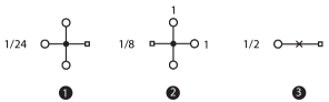
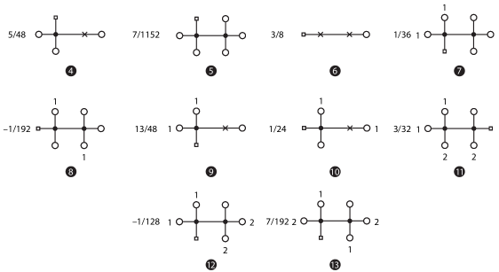
Figure 1: Rooted tree-diagrams contributing at $O(g_{0})$; note that $\delta m^{2}=O(g_{0})$.

Figure 2: Rooted tree-diagrams contributing at $O(g_{0}^{2})$; note that $\delta m^{2}=O(g_{0})$.

Black circles and crosses represent the vertices of the theory: they are the usual $\varphi^{4}$ vertex and mass counterterm insertions,

$$\includegraphics[scale={0.3},trim=0.0pt 35.13124pt 0.0pt 0.0pt]{Vertex}=-1,\qquad\includegraphics[scale={0.2},trim=0.0pt 20.075pt 0.0pt 0.0pt]{Counterterm}=1.$$ (3.23)

These are associated with implicit factors of $-g$ and $\delta m^{2}$ respectively. Black lines connecting two vertices correspond to the scalar propagator,

$$\includegraphics[scale={0.2},trim=0.0pt -3.01125pt 0.0pt 0.0pt]{Propagator}=G(x,y)=\frac{1}{L^{4}}\sum_{p\in{\tilde{\Omega}}}e^{ip(x-y)}{\tilde{G}}(p),$$ (3.24)

where $x$ and $y$ are the positions of the two vertices connected by the given propagator. In particular, at each vertex the fields attached are multiplied together and the propagator is applied to the resulting product of fields.

The root of the diagram is given by

$$\includegraphics[scale={0.25},angle={180},trim=0.0pt 38.14249pt 0.0pt 0.0pt]{Root}=G(x,y),$$ (3.25)

where $x$ is the space-time index of the corresponding rooted tree $\mathcal{R}_{i}$.

To give some examples, given some $\eta_{0}(x)$ and $\eta_{1}(x)$ fields, the diagram labeled ❷ in Figure 2 evaluates to

$$v(x,\mathcal{R}_{2})=(-1)\,\sum_{y\in\Omega}G(x,y)\chi_{0}(y)\chi_{1}(y)^{2}.$$ (3.26)

This contributes to $\phi_{1,0}(x)$ with a coefficient $c(\mathcal{R}_{2})=1/8$. Diagram ❹ in Figure 2, stands for

$$v(x,\mathcal{R}_{4})=(-1)\,\sum_{y\in\Omega}G(x,y)\chi_{0}(y)^{2}\sum_{z\in\Omega}G(y,z)\chi_{0}(z),$$ (3.27)

and contributes to $\phi_{1,1}(x)$ with $c(\mathcal{R}_{4})=5/48$.

$g_{0}^{k}$	$n$	$c(\mathcal{R})\neq 0$
1	3	3
2	10	10
3	44	43
4	241	231
5	1,506	1,420
6	10,778	10,015
Total	12,582	11,722

Table 1: Number of rooted-tree diagrams appearing at a given order in the coupling $g_{0}$. The column labeled by $c(\mathcal{R})\neq 0$ gives the number of such diagrams whose coefficient $c(\mathcal{R}_{i})$ is non-vanishing.

Given these examples it is clear that the evaluation of the trivializing map for a given set of random fields $\eta_{i}$ is in principle straightforward. Beyond the lowest perturbative orders though the number of diagrams (as well as their complexity) increases rapidly as indicated in Table 1, so the computation must be automated.

For this work we wrote a program that evaluates the trivializing field $\phi(x)$ up to an arbitrary order $N$ in the couplings for a given set of $\eta_{i}$ fields. For the structure of the relevant diagrams and the determination of their coefficients we used the software package provided by Martin Lüscher [20]. The diagrams are given as C structs of abstract elements, so our program visits each vertex in a diagram using depth-first recursion starting from the root, and evaluates the corresponding numerical expressions. The diagrams are collected according to their order in the couplings and the $\phi_{k,l}(x)$ fields are thus constructed. This allows the series (3.18) to be obtained for some set of $\eta_{i}$ fields. Once this is done, correlation functions of the trivializing field can be expanded order by order in the couplings and evaluated stochastically by averaging over different samples of the Gaussian random fields $\eta_{i}$. In particular, the perturbative expansion of generic observables of the trivializing field ${\cal O}(\phi)$ can be computed by iterating order by order convolution operations of the form,

$$(\phi\cdot\phi)(x,y)=\phi(x)\phi(y)\quad\Longrightarrow\quad(\phi\cdot\phi)_{k,\ell}(x,y)=\sum_{0\leq i\leq k}\sum_{0\leq j\leq\ell}\phi_{k-i,\ell-j}(x)\phi_{i,j}(y),$$ (3.28)

and similarly for other elementary operations. In this way one obtains the generic stochastic perturbative field,

$${\cal O}(\phi)=\sum_{k,\ell=0}^{N}{\cal O}_{k,\ell}(\phi_{0,0},\ldots,\phi_{k,\ell})\,g_{0}^{k}(\delta m^{2})^{\ell}+O(g_{0}^{N+1}),$$ (3.29)

from which the perturbative expansion of the expectation value of the field ${\cal O}(\varphi)$ in $\varphi^{4}$ theory,

$$\langle{\cal O}\rangle=\sum_{k,\ell=0}^{N}a_{k,\ell}\,g_{0}^{k}(\delta m^{2})^{\ell}+O(g_{0}^{N+1}),$$ (3.30)

is obtained up to $O(g_{0}^{N+1})$ corrections as

$$\langle{\cal O}\rangle_{\eta}=\langle{\cal O}\rangle\quad\iff\quad\langle{\cal O}_{k,\ell}\rangle_{\eta}=a_{k,\ell}.$$ (3.31)

Once the expansion (3.29) is known the corresponding expansion in terms of a given renormalized mass and coupling (as well as any renormalization of the field ${\cal O}$) is easily found (q.v., Appendix A).

We should mention some additional technical details. First, in the diagrammatic computation the scalar propagators are applied in momentum space, while the products of fields at vertices are performed in position space. This is implemented using the efficient numerical evaluation of the discrete Fourier transformation provided by the FFTW package [21]. As a result the cost of the computation of the diagrams scales proportionally to the system size $V=L^{4}$ up to logarithms. Second, as already noted in [12], the computation of the rooted tree diagrams could be organized in such a way that identical sub-trees in different graphs are cached. How to do this efficiently is a non-trivial issue even for $\varphi^{4}$ theory, and we did not investigate it further. Moreover, whether this is really worth investigating is not clear since, as we shall see below, ISPT suffers from some severe limitations once high-order computations are considered. Its utility might thus be limited to relatively low-order computations where recomputation of subgraphs is not a significant issue.

The advantages of ISPT are that its results are exact up to statistical uncertainties and that there are no autocorrelations as the coefficients $\phi_{k,\ell}$ are generated “instantaneously” from independent Gaussian random fields $\eta_{i}$.

3.2 A test of the method

We tested our ISPT implementation by comparing some results with those obtained using conventional perturbative lattice calculations (LPT). We computed the renormalized coupling (2.10) and compared it with its two-loop determination from [14], which we evaluated for the parameters of interest (see below). We considered both the case where the perturbative expansion is given in terms of the renormalized mass (2.7), and the case where it is given in terms of the bare mass $m_{0}$. The comparison was done on a tiny lattice with $L=4$, where high statistics could be gathered, and the value of the mass was chosen such that $z=4$. The results of the tests are reported in Table 2; for completeness we also give the results for $\delta m^{2}$ in the table.

	Mass	$c_{2}\times 10^{2}$	$c_{3}\times 10^{3}$	$m^{2}_{1}\times 10^{2}$	$m^{2}_{2}\times 10^{4}$
LPT	$m$	$-3.330$	$1.583$	$-6.4221$	$3.6702$
ISPT	$m$	$-3.332(6)$	$1.582(4)$	$-6.4220(1)$	$3.6704(6)$
LPT	$m_{0}$	$-3.33$	$2.965$
ISPT	$m_{0}$	$-3.33(1)$	$2.964(5)$

Table 2: Results for the series (2.3) and (2.2) as obtained from ISPT and conventional LPT for $L=4$ and $z={\rm Mass}\times L$ using $10^{8}$ field configurations. The perturbative expansion for the coupling (2.3) is obtained both in terms of the renormalized mass $m$ of (2.7) and the bare mass $m_{0}$.

As can be seen from the table there is good agreement between the ISPT and the LPT determinations, thus confirming the correctness of our implementation. In the case where the mass renormalization is considered one needs to take into account the effect of statistical errors in the mass renormalization procedure discussed in Appendix A.2: we did this using the jackknife method.

4 NSPT based on the Langevin equation

Having introduced ISPT, in this and the following section we discuss the other NSPT methods that we studied. In these methods the stochastic field $\phi$ is generated through a Markov process based on some stochastic differential equation expanded up to some fixed order in the couplings of the theory. We start from the standard NSPT based on the Langevin equation; for later convenience we shall refer to this algorithm as LSPT. This algorithm has a long history and has been studied in great detail over the years: we thus limit ourselves to recalling the most relevant features for what follows, while referring the reader to the literature for a more detailed account (see, e.g., [6] and references therein).

4.1 Definition

The standard LSPT approach is based on stochastic quantization [10, 22, 23, 24, 11], where the field representing the theory is obtained as the solution of the Langevin equation,

$$\partial_{t_{s}}\phi(t_{s},x)=-F\bigl{(}\phi(t_{s},x)\bigr{)}+\eta(t_{s},x),$$ (4.32)

where $F(\bigl{(}\phi(t_{s},x)\bigr{)}$ denotes the functional derivative of the action (2.1) evaluated on the field configuration $\phi(t_{s},x)$,

$$F\bigl{(}\phi(t_{s},x)\bigr{)}=\frac{\delta S[\phi]}{\delta\phi(t_{s},x)}=-\partial^{2}\phi(t_{s},x)+(m^{2}+\delta m^{2})\phi(t_{s},x)+\frac{g_{0}}{3!}\phi(t_{s},x)^{3}.$$ (4.33)

We have written the bare mass $m_{0}$ in terms of the renormalized mass and its counterterm (q.v., (2.2)). In the above equations $t_{s}$ is the so called stochastic (or simulation) time in which the stochastic field $\phi$ evolves. The field $\eta$ is a field of Gaussian random numbers satisfying

$$\bigl{\langle}\eta(t_{s},x)\bigr{\rangle}_{\eta}=0,\qquad\bigl{\langle}\eta(t_{s},x)\eta(t_{s}^{\prime},y)\bigr{\rangle}_{\eta}=2\delta(t_{s}-t_{s}^{\prime})\delta_{xy}.$$ (4.34)

Through the Langevin equation (4.32) the field $\phi$ depends upon the random field $\eta$. The main assertion of stochastic quantization is that the following identity holds order by order in perturbation theory:

$$\lim_{t_{s}\to\infty}\bigl{\langle}\phi(t_{s},x_{1})\cdots\phi(t_{s},x_{n})\bigr{\rangle}_{\eta}=\bigl{\langle}\varphi(x_{1})\cdots\varphi(x_{n})\bigr{\rangle}.$$ (4.35)

Hence, in the long stochastic time limit the equal time correlation functions of the stochastic field $\phi$ converge to the expectation values (2.4) of the Euclidean field theory with action $S$; in particular the equilibrium probability distribution of the stochastic field $\phi$ is proportional to $e^{-S(\phi)}$. Equivalently, one can say that in this limit the Langevin equation effectively trivializes the original theory (q.v., (3.15)).

Stochastic perturbation theory amounts to solving the Langevin equation (4.32) order by order in the couplings of the theory; in our case these are $g_{0}$ and $\delta m^{2}$. Substituting the expansion of the stochastic field $\phi$ analogous to (3.18) into (4.32) gives a system of equations for the fixed order fields,

$$\begin{split}\partial_{t_{s}}\phi_{0,0}(t_{s},x)&=(\partial^{2}-m^{2})\phi_{0,0}(t_{s},x)+\eta(t_{s},x),\\ \partial_{t_{s}}\phi_{1,0}(t_{s},x)&=(\partial^{2}-m^{2})\phi_{1,0}(t_{s},x)-\frac{1}{3!}\phi_{0,0}(t_{s},x)^{3},\\ \partial_{t_{s}}\phi_{0,1}(t_{s},x)&=(\partial^{2}-m^{2})\phi_{0,1}(t_{s},x)-\phi_{0,0}(t_{s},x),\end{split}$$ (4.36)

and so on. These equations can readily be solved for the $\phi_{k,\ell}$ fields. Once a solution is obtained up to a given order in the coupling, (4.35) can be used to compute the perturbative expansion of any correlation function in the corresponding Euclidean field theory (see [11] for explicit examples of such calculations).

LSPT is the numerical implementation of this idea. Stochastic time is discretized as $t_{s}=n\varepsilon$, with $n\in\mathbb{N}$ and $\varepsilon$ being the step-size; a solution of the (discrete) Langevin equation is then obtained according to some given integration scheme. The simplest such solution is provided by the Euler scheme, which is defined by the update step

$$\phi\bigl{(}(n+1)\varepsilon,x\bigr{)}=\phi(n\varepsilon,x)-\varepsilon F\bigl{(}\phi(n\varepsilon,x)\bigr{)}+\sqrt{\varepsilon}\,\eta(n\varepsilon,x),$$ (4.37)

where here the random field $\eta$ is normalized such that $\bigl{\langle}\eta(n\varepsilon,x)\eta(n^{\prime}\varepsilon,y)\bigr{\rangle}_{\eta}=2\delta_{nn^{\prime}}\delta_{xy}$, and $\phi(0,x)$ is some given initial condition. The perturbative expansion of this solution is performed in an automated fashion by employing order by order operations analogous to (3.28); once this is given the expansion of a generic observable ${\cal O}\bigl{(}\phi(t_{s})\bigr{)}$ is obtained in the same way as in (3.29). Assuming ergodicity the average over the random field distribution in (4.35) is replaced by an average over stochastic time, and one obtains

$$\lim_{t_{s}\to\infty}\bigl{\langle}{\cal O}(t_{s})\bigr{\rangle}_{\eta}=\langle{\cal O}\rangle\quad\xrightarrow{t_{s}=n\varepsilon}\quad\lim_{T\to\infty}\frac{1}{T}\sum_{n=0}^{T}{\cal O}\bigl{(}\phi(n\varepsilon)\bigr{)}=\langle{\cal O}\rangle+O(\varepsilon^{p}).$$ (4.38)

In the above relation the equivalence between correlation functions is valid order by order in perturbation theory (q.v., (3.31)), whereas the power $p$ depends on the order of the chosen integration scheme (see below).

As asserted earlier, stochastic estimates of perturbative expansions of the correlation functions of the target theory are obtained by use of Monte Carlo sampling based on the Langevin equation. We note that within the statistical uncertainties the perturbative expansions so obtained are correct only up to systematic errors due to the discretization of the stochastic time. As anticipated in (4.38) these corrections are expected to vanish as some power of the step-size as $\varepsilon\to 0$ [25, 26]. The rate of convergence depends on the choice of the numerical integrator employed for the solution of the Langevin equation. Such integrators are normally devised in such a way that the discrete stochastic process associated with the given integration scheme of order $p$ converges, for small enough $\varepsilon$, to an equilibrium probability distribution $\bar{P}(\phi)\propto e^{-\bar{S}(\phi)}$ where $\bar{S}=S+\Delta S$ with $\Delta S=O(\varepsilon^{p})$. Such deviation from the desired equilibrium distribution is the cause of the corrections in the expectation value in (4.38) (see, e.g., [26, 27] for more details). In this work we used a second order Runge–Kutta integrator (RK2): its exact definition is given by eqs. (A.4) and (A.15) of [28]. Using this integrator one expects corrections of $O(\varepsilon^{2})$ in the perturbative computation of any correlation function.

It is clear that compared to ISPT the cost of LSPT with the perturbative order in the couplings is rather mild. This is dictated by the order-by-order operations necessary to integrate the discrete Langevin equation. Consequently, the computational cost of LSPT increases (roughly) with the square of the order in each coupling (q.v., (3.28)). However, as just mentioned, the results need to be extrapolated to zero in the step-size to eliminate systematic errors in the results. In addition, as the fields entering in the average in (4.38) are generated by a Markov process, the successive field configurations are correlated; this increases the statistical error for a fixed number of field configurations. These correlations need to be properly taken into account in order to obtain valid error estimates for the results. Their magnitude is expected to grow proportionally to $L^{2}$ as the continuum limit of the theory is approached (see, e.g., [26, 29, 30]). This result is valid for any perturbative order ${\cal O}_{k,\ell}\bigl{(}\phi_{0,0}(t_{s}),\ldots,\phi_{k,\ell}(t_{s})\bigr{)}$ of the generic (multiplicatively renormalizable) stochastic field ${\cal O}\bigl{(}\phi(t_{s})\bigr{)}$, and follows from the remarkable property that the Langevin equation is renormalizable [23, 24] (see [30] for a discussion). This feature allows one to infer the scaling behavior of Langevin-based algorithms not only in the free case where $g_{0}=0$ but also in the full interacting theory. In particular, as recently shown by Martin Lüscher [31], the renormalizability of the Langevin equation also allows one to conclude that the variances of these coefficients, ${\mathop{\rm Var}}({\cal O}_{k,l})=\lim_{t_{s}\to\infty}\left(\bigl{\langle}{\cal O}_{k,\ell}^{2}(t_{s})\bigr{\rangle}_{\eta}-\bigl{\langle}{\cal O}_{k,\ell}(t_{s})\bigr{\rangle}_{\eta}^{2}\right)$, are at most logarithmically divergent when taking the continuum limit. This property is quite remarkable and is not guaranteed for other NSPT implementations.

5 NSPT based on GHMD algorithms

The idea of stochastic perturbation theory is not limited to the Langevin equation. Any stochastic differential equation (SDE) which satisfies an analogous property to (4.35) can provide a way of performing stochastic perturbation theory. One interesting example is given by the stochastic molecular dynamics (SMD) equations (5.41). In this context these were first considered in [32], and were recently studied in detail in [30]. Similarly, one can set-up perturbation theory in terms of the Hybrid Molecular Dynamics (HMD) equations [30]. This observation suggests the possibility of defining NSPT based on the discretization of these SDEs or of ergodic variances of the molecular dynamics (MD) equations; such as the Kramers [33, 34, 35, 36] and HMD algorithm respectively [37]. Experience with conventional non-perturbative lattice field theory simulations would suggest the advantages of reformulating NSPT in terms of these algorithms rather than Langevin-based ones. However determining their efficiency in this context, in particular their continuum scaling, is not a trivial issue. The results for the free field theory [38] provide a complete understanding of the lowest perturbative order dynamics. On the other hand the lack of renormalizability of the SMD and HMD equations [30] in general precludes analytic control over the continuum scaling of these algorithms in the interacting theory. In the case of NSPT this means a lack of control of the behaviour of the higher-order fields. Consequently, the efficiency of these algorithms in the context of NSPT must be addressed numerically; in particular the situation could be substantially different from both the free case and the case where the full theory is simulated.

In this section we define NSPT in terms of the HMD and Kramers algorithms (see [38] and references therein for their definition). These are all inexact algorithms, as we do not know how to add a Metropolis step that would be valid for arbitrary values of the coupling beyond leading (free field) order. We could consider the more general Generalized Hybrid Molecular Dynamics algorithm [38], but based on both the expectations from free field theory and from non-perturbative lattice field theory simulations the HMD and Kramers algorithms appear to be natural sub-classes of the GHMD algorithm to consider. We shall assume the reader to be familiar with these algorithms, and we limit ourselves to describing the required modifications for their NSPT formulations. These algorithms will be called HSPT and KSPT, respectively.

5.1 HSPT

In the case of the HMD algorithm, the basic field evolution is described by the MD equations,

$$\partial_{t_{s}}\phi(t_{s},x)=\pi(t_{s},x),\qquad\partial_{t_{s}}\pi(t_{s},x)=-F\bigl{(}\phi(t_{s},x)\bigr{)},$$ (5.39)

where $F\bigl{(}\phi(t_{s},x)\bigr{)}$ is given by (4.33), and $\pi$ is the momentum field conjugate to $\phi$. Similarly to the Langevin case (cf. §4), in the context of NSPT both fields $\phi$ and $\pi$ are assumed to have an expansion of the form (3.18). All operations in the following are thus intended to be performed in an order by order fashion (q.v., (3.28)).

As is well known an algorithm based on the MD equations alone conserves “energy” and so is not ergodic: the latter needs to be supplemented by an occasional refreshment of the momentum field. Therefore the momentum field $\pi$ is sampled from a Gaussian distribution with zero mean and unit variance at the beginning of each trajectory ($t_{s}=t_{0}$); the refreshed momentum initially only has a non-zero lowest order component. In formulas

$$\bigl{\langle}\pi_{0,0}(t_{0},x)\bigr{\rangle}_{\pi}=0,\qquad\bigl{\langle}\pi_{0,0}(t_{0},x)\pi_{0,0}(t_{0},y)\bigr{\rangle}_{\pi}=\delta_{xy},$$ (5.40)

and $\pi_{k,\ell}(t_{0},x)=0$ if either $k>0$ or $\ell>0$, where $\langle\cdots\rangle_{\pi}$ denotes the average over the momentum field distribution at the beginning of a trajectory. The momentum field will acquire higher-order components during the MD evolution (5.39) from the time $t_{0}$ at which it was refreshed to time $t_{s}=t_{0}+\tau$, where $\tau$ is the trajectory length. Numerically the MD evolution is determined by discretizing the simulation time as $t_{s}=n\delta t$, with $n\in\mathbb{N}$ and $\delta t$ the step-size, and employing a suitable integration scheme (see below). Expectation values of generic observables are then obtained similarly to (4.38) by averaging over sequences of trajectories.

For the numerical integration of the MD equations it is convenient to rely on some reversible symplectic integration scheme, even though this is not necessary in principle. Symplectic integrators can systematically be improved, and sophisticated symplectic integrators are readily available (q.v., [39] for a discussion). Moreover, once an efficient symplectic integrator is found for a scalar theory, it can be extended to non-Abelian theories in a straightforward manner. For this work we used the fourth order integrator defined by equations (63) and (71) of [40], which we refer to as the OMF4 integrator. Given this choice of integrator we expect $O(\delta t^{4})$ errors in the results. More precisely, we expect in general that the equilibrium probability distribution of fields generated through the HMD algorithm with some symplectic integrator of order $p$ is, for small enough step-size $\delta t$, of the form $\bar{P}(\phi)\propto e^{-\bar{S}(\phi)}$, where $\bar{S}=S+\Delta S$ with $\Delta S=O(\delta t^{p})$ (see [41] for more details). Consequently, since $\Delta S\propto V$, one may argue that in order to keep the step-size errors in the equilibrium distribution (approximately) constant as the system size $V$ is increased, one needs to keep the quantity $y\equiv V\delta t^{p}$ fixed. It is clear that this is feasible only if efficient high-order integrators are employed. We note that although keeping $y$ fixed would keep systematic errors in generic correlators approximately constant as the system size is increased, this is probably an over-conservative condition if one is interested in (connected) correlation functions of local fields [25, 26].

The HSPT algorithm described so far is not yet ergodic, the problem being that the evolution of the lowest-order (free) field $\phi_{0,0}$ is not ergodic [42, 38]; this in turn affects the evolution of the higher-orders. The solution to this problem is simple and is to randomize the trajectory length $\tau$ [42]. The choice of distribution for the trajectories lengths may affect the efficiency of the algorithm. In our implementation we fixed the step-size $\delta t$, while choosing the number of steps $n$ composing the trajectory according to a binomial distribution with mean $\langle n\rangle$. This defines the average trajectory length to be $\langle\tau\rangle=\langle n\rangle\delta t$.

We conclude by pointing out that if one chooses $\tau=\delta t$, i.e., the trajectory consists of a single step, then the HMD algorithm effectively integrates the Langevin equation (4.32) (q.v., [41] and below). In other words, in this case the algorithm just described can be interpreted as a particular integration scheme for the Langevin equation.

5.2 KSPT

Having defined HSPT in terms of the HMD algorithm, a second interesting possibility to consider is NSPT based on the Kramers algorithm. This algorithm was proposed long ago in the context of field theory simulations by Horowitz [33, 34], and recently reconsidered in [36]. In this case, the stochastic equations governing the fields dynamics are given by the SMD equations,

$$\partial_{t_{s}}\phi(t_{s},x)=\pi(t_{s},x),\qquad\partial_{t_{s}}\pi(t_{s},x)=-\gamma\pi(t_{s},x)-F\bigl{(}\phi(t_{s},x)\bigr{)}+\eta(t_{s},x).$$ (5.41)

Here $F\bigl{(}\phi(t_{s},x)\bigr{)}$ is still defined by (4.33), while $\eta(t_{s},x)$ is a Gaussian random field satisfying

$$\bigl{\langle}\eta(t_{s},x)\bigr{\rangle}_{\eta}=0,\qquad\bigl{\langle}\eta(t_{s},x)\eta(t_{s}^{\prime},y)\bigr{\rangle}_{\eta}=2\gamma\delta(t_{s}-t_{s}^{\prime})\delta_{xy},$$ (5.42)

where $\gamma>0$ is a free parameter (see below). We observe that the (non-ergodic) MD equations (5.39) are obtained when $\gamma=0$ while, up to a rescaling of stochastic time, the Langevin equation (4.32) is obtained for $\gamma\to\infty$ (q.v., [30]).

The implementation of Kramers algorithm is as follows. Starting from some arbitrary initial values for the fields $\phi(0,x)$ and $\pi(0,x)$, the MD equations corresponding to (5.41) with $\gamma=0$ are integrated from $t_{s}=0$ to $t^{\prime}_{s}=\delta t$ through a single step of a given numerical integration scheme. The value of $\delta t$ thus defines the step-size of the integrator. After this MD step, the effect of the $\gamma$ term and the coupling to the random field $\eta$ is taken into account by partially refreshing the momentum field: the momentum field $\pi(t^{\prime}_{s},x)$ is replaced by

$$\pi^{\prime}(t^{\prime}_{s},x)=e^{-\gamma\delta t}\pi(t^{\prime}_{s},x)+\sqrt{1-e^{-2\gamma\delta t}}\,\eta(t^{\prime}_{s},x),$$ (5.43)

where the noise field is here normalized such that $\bigl{\langle}\eta(n\delta t,x)\eta(n^{\prime}\delta t,y)\bigr{\rangle}_{\eta}=\delta_{nn^{\prime}}\delta_{xy}$. These elementary steps are then alternated, and expectation values of generic observables of the field are obtained as in (4.38) by averaging over a long Monte Carlo history, after they have reached equilibrium. In a KSPT implementation, the fields $\phi$ and $\pi$ are assumed to have an expansion of the form (3.18), and just as in the Langevin case the random field $\eta$ only has a lowest-order component. Hence, during the partial refreshment (5.43) only the lowest-order component of the momentum field $\pi_{0,0}$ is affected by the random field $\eta$, while the higher-order components are just rescaled by the factor $e^{-\gamma\delta t}$. In the case where $\gamma\to\infty$ (the Langevin limit) the algorithm described is just the single step HSPT algorithm.

Having defined the algorithm, some comments are in order. First of all, as shown by Horowitz’s analysis [33], the partial momentum refreshment (5.43) integrates exactly the corresponding terms in (5.41). Similarly to the case of HSPT, the systematic errors that one expects in expectation values of the fields (4.38) are given by the integration of the MD equations in discrete steps; in particular analogous conclusions apply for the order of the step-size errors in the equilibrium probability distribution (q.v., §5.1). For the present work, we employed the very same OMF4 integrator that we used for HSPT: we therefore expect $O(\delta t^{4})$ step-size errors.

Secondly, one might naïvely conclude from the free field theory analysis of [38] that the KSPT algorithm just defined is not of much interest as it is not expected to perform better than HSPT, at least close to the continuum limit. However, one has to note that the conclusions in [38] refer to the exact implementation of these algorithms, i.e., when a Metropolis accept/reject step is included. This is what leads to the critical exponent for the cost of the algorithms being $z=1$ for HMC but $z=3/2$ for the exact Kramers algorithm (KMC). However, in the case of NSPT one is limited to inexact algorithms, so the computations have to be performed in a parameter regime where the effect of step-size errors on expectation values are smaller than some specified statistical accuracy, as otherwise some extrapolation in the step-size would be necessary. In this regime, corresponding to the case where the Metropolis acceptance probability would be close to one, the two algorithms have in fact comparable performances [38].

KSPT is also interesting due to the following property. As mentioned before, the SMD equations (5.41) approach the Langevin equation (4.32) in the limit $\gamma\to\infty$. In lattice field theory, this limit can be taken simultaneously with the continuum limit if $\gamma$ is kept fixed in lattice units while $a\to 0$ [30]. In this limit the algorithm described above integrates the Langevin equation as the continuum limit of the theory is approached. Consequently, the considerations on the continuum scaling of the LSPT algorithms discussed in §4 directly apply to KSPT at fixed $\gamma$. Although the scaling of these algorithms is expected to be the same, in the case of KSPT the parameter $\gamma$ may be fixed to some finite value for which the algorithm may be more efficient. This will be addressed in detail in the next section.

6 Numerical results

In this section we present the results of our numerical investigation of the methods described in §3—§5. Our aim is to provide a comparison of the techniques in order to identify their principal advantages and disadvantages. In §6.1 we compare the perturbative results for some specific quantities obtained with the different algorithms, in order to confirm their correctness and viability. Once these are established, in §6.2—§6.5 we study the continuum scaling of the errors of these perturbative coefficients as computed by the various methods.

6.1 Testing the methods

Before other comparisons are considered it is important to confirm that the various algorithms agree for the perturbative computation of some quantities. In Figure 3 the results for $\mathcal{E}(t)$ at tree-level, $O(g_{0})$, and $O(g_{0}^{2})$ are shown from top to bottom respectively. The computations were performed on a tiny $L=4$ lattice for which very high statistics could be obtained: similar results were obtained on larger lattices albeit with lower precision. We collected $\approx 10^{7}$ independent measurements for ISPT, HSPT, and KSPT, and $\approx 10^{6}$ measurements for each of 9 values of $\varepsilon\in[0.01,0.05]$ for LSPT. The values for the mass of the field and the flow time were chosen to correspond to $z=4$ and $c=0.2$, respectively. For HSPT and KSPT we then chose $\langle\tau\rangle=1$ and $\gamma=2$. The perturbative expansion is expressed in terms of the renormalized mass $m$ whereas the perturbative coefficients correspond to the expansion in the bare coupling $g_{0}$, i.e.,

$$\mathcal{E}(L,z,c)=\mathcal{E}_{0}+\mathcal{E}_{1}g_{0}+\mathcal{E}_{2}g_{0}^{2}+\mathcal{E}_{3}g_{0}^{3}+O(g_{0}^{4}),\quad\mbox{where}\quad\mathcal{E}_{i}\equiv\mathcal{E}_{i}(L,z,c).$$ (6.44)

As can be seen from the figure, all the methods agree with each other and with the analytic determination. In the case of LSPT deviations from the expected results are sizable at the largest step-sizes, and agreement is found only after extrapolation to $\varepsilon\to 0$. In particular, the asymptotic $O(\varepsilon^{2})$ behaviour expected for the integrator used is clearly visible.

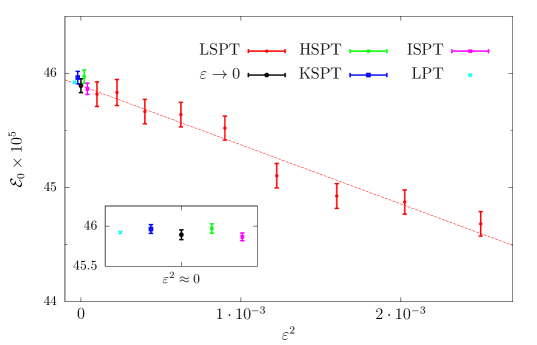
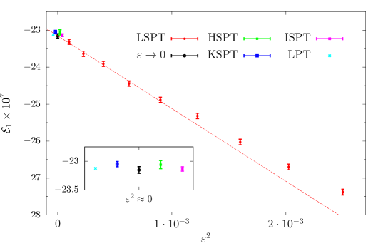
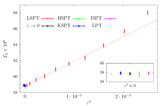
Figure 3: Comparison of different methods in the determination of $\mathcal{E}_{0}$, $\mathcal{E}_{1}$ and $\mathcal{E}_{2}$ for $z=4$, $c=0.2$, and $L=4$. The analytic result (LPT) and the result of the extrapolation $\varepsilon\to 0$ for LSPT, as well as the ISPT, KSPT, and HSPT results (for which there are no step-size errors or the step-size errors are negligible compared with the statistical errors) are plotted near $\varepsilon^{2}=0$.

For the case of HSPT and KSPT we do not see any indication of step-size errors as the results show no statistically significant deviation from the analytic determination; the points are precise at the $0.1$–$0.5\%$ level depending on the order. Even though the lattice is quite small, the step-size we chose for both HSPT and KSPT is rather large, namely $\delta t=0.5$. This step-size satisfies $\delta t^{4}\geq 25\,\varepsilon^{2}$, for all values of $\varepsilon$ considered for LSPT: this inequality would give the naïve size of the expected relative step-size errors. This needs to be compared with the fact that the application of the OMF4 integrator only costs twice as much computer time as the RK2 integrator. Of course this result depends on many factors: the lattice size considered, the observable, the parameters of the theory, the values of the step-sizes, and most importantly the integrators used. Nonetheless, as already emphasized, symplectic MD integrators are at a more mature stage of development than Runge Kutta integrators; they can be optimized to reduce the magnitude of the step-size errors (q.v., [40]). As illustrated by our example, this results in a significant reduction of systematic errors relative to the cost of a single integration step. Consequently, it is feasible to run the algorithm with a small enough step-size such that extrapolations are not required. Moreover, as we can afford to run with larger step-sizes for a fixed systematic error and with a fixed number of force computations the cost of obtaining independent configurations is reduced because of the smaller autocorrelations. Later in the section we shall give more quantitative evidence on the benefits of using efficient symplectic integrators in minimizing both systematic and statistical errors at fixed cost.

6.2 Continuum error scaling: a first look

Having addressed the issue of systematic errors, we now study the continuum scaling of the various NSPT algorithms. We do this by investigating how the (relative) errors of the perturbative coefficients of some given observables scale as the continuum limit of the theory is approached. The precise details of the scaling depend on the observable, but some general features may be inferred.

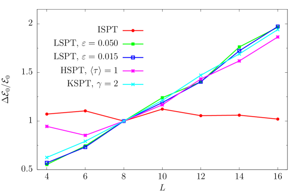
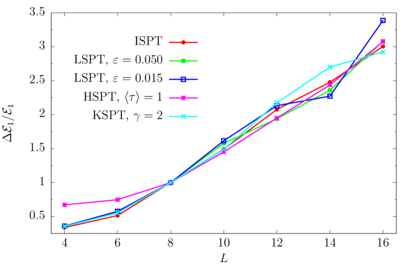
Figure 4: Continuum scaling of the relative errors $\Delta\mathcal{E}_{0}/\mathcal{E}_{0}$ and $\Delta\mathcal{E}_{1}/\mathcal{E}_{1}$ as computed with ISPT, LSPT, HSPT, and KSPT. The parameters are $z=4$ and $c=0.2$. The data is normalized at $L=8$.

In Figures 4 and 5 we show the continuum scaling of the relative errors $\Delta\mathcal{E}_{i}/\mathcal{E}_{i}$ for $i=0,\ldots,3$ and $L$ in the range $4\leq L\leq 16$, as computed using ISPT, LSPT, HSPT, and KSPT. Recall that the error $\Delta\mathcal{E}_{i}$ may be expressed as

$$\Delta\mathcal{E}_{i}=\sqrt{\frac{2A_{I}(E_{i})\times\mathop{\rm Var}(E_{i})}{N_{\mbox{\tiny config}}}},$$ (6.45)

where $N_{\mbox{\tiny config}}$ is the total number of field configurations considered, and ${\rm Var}(E_{i})$ and $A_{I}(E_{i})$ are the variance and integrated autocorrelation of $E_{i}$ where

$$\frac{t^{2}}{L^{4}}\sum_{x\in\Omega}E(t,x)={E_{0}}+E_{1}g_{0}+E_{2}g_{0}^{2}+E_{3}g_{0}^{3}+O(g_{0}^{4}).$$ (6.46)

We show our results for $z=4$ and $c=0.2$, but the same qualitative behaviour is observed in other cases. The number of configurations for each method is specified at $L=4$ and kept constant as $1/L\to 0$. Specifically, at $L=4$ we collected between $10^{5}$ and $10^{6}$ independent measurements for each of the different methods. At this small lattice size and for the algorithmic parameters considered the different methods have comparable statistical precision for the same number of independent measurements. In the case of LSPT we measured after each step of the Markov chain. For KSPT we set the parameter $\gamma=2$, and we adjusted the measurement frequency so as to measure at fixed intervals $\Delta t_{s}=0.5$ of simulation time independent of the step-size. For HSPT we measured after each trajectory of average length $\langle\tau\rangle=1$. The results in the figures are normalized to the values of the relative errors at $L=8$, and hence to a first approximation are independent of $N_{\mbox{\tiny config}}$. Since the figures are only intended to be qualitative no estimates for the error on the relative error are provided.

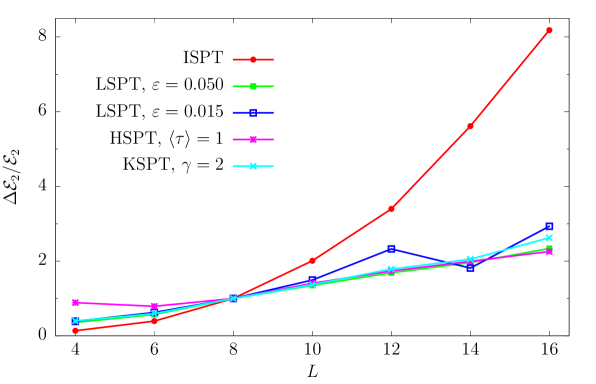
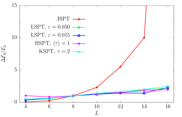
Figure 5: Continuum scaling of the relative errors $\Delta\mathcal{E}_{2}/\mathcal{E}_{2}$ and $\Delta\mathcal{E}_{3}/\mathcal{E}_{3}$ as computed with ISPT, LSPT, HSPT, and KSPT. The parameters are $z=4$ and $c=0.2$. The data is normalized at $L=8$. Note that for ISPT $\Delta\mathcal{E}_{3}/\mathcal{E}_{3}\approx 65$ for $L=16$.

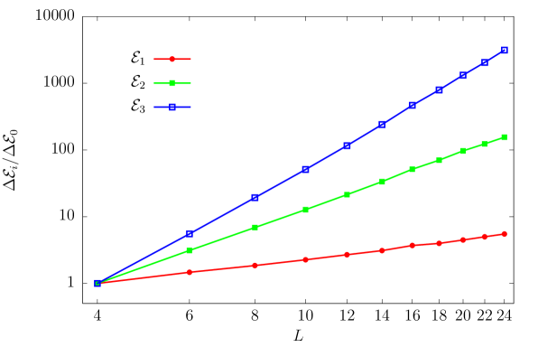
Figure 6: Continuum scaling of the ratios $\Delta\mathcal{E}_{i}/\Delta\mathcal{E}_{0}$ for $i=1,2,3$ as computed with ISPT. The case with $z=4$ and $c=0.2$ is shown. The results are normalized to their values at $L=4$.

The error computation for the perturbative coefficients was obtained using jackknife in the case of ISPT, whereas for LSPT, HSPT, and KSPT we employed the $\Gamma$-method described in [43] in order to take into account autocorrelations of the measured quantities. The coefficients $\mathcal{E}_{i}$ and corresponding errors refer to the expansion in terms of the renormalized mass $m$ and bare coupling $g_{0}$ (6.44). Power divergences in the inverse lattice spacing are thus excluded in the coefficients $\mathcal{E}_{i}$, while logarithmic divergences associated with renormalization of the coupling constant are not expected to be relevant for the following discussion. In the case of HSPT and KSPT the step-size was scaled as $\delta t\propto 1/L$ starting from a value of $\delta t=0.5$ so as to keep the $O(\delta t^{4})$ errors in the equilibrium distribution approximately fixed using the OMF4 integrator as the continuum limit is approached. As mentioned in §5.1 this is probably a very conservative choice, but it was done to avoid potentially large systematic errors that might modify the overall picture. Keeping the systematic errors in the equilibrium distribution fixed for LSPT is significantly more challenging as it requires $\varepsilon\propto 1/L^{2}$ with the RK2 integrator (q.v., §4). In this case we thus simply considered two well-separated step-sizes in order to assess the dependence of the results on $\varepsilon$.

Starting from the results at tree-level (top panel in Figure 4) we see how the relative error of ISPT is constant for a fixed number of field configurations. The results for LSPT, HSPT, and KSPT are rather different: excluding perhaps the smaller lattices there is a linear growth of the relative errors with the lattice size. These results confirm free field theory expectations. The variance $\mathop{\rm Var}(E_{0})$ is finite and constant with $L$ up to discretization effects. In particular it is the same for all NSPT methods up to step-size errors, and independent of the algorithmic parameters. Consequently, since ISPT results are uncorrelated, this implies that the error $\Delta\mathcal{E}_{0}$ is essentially constant with $L$ for a given number of field configurations $N_{\mbox{\tiny config}}$. The linear rise of the errors in the case of LSPT, HSPT, and KSPT is due to the fact that autocorrelations grow $\propto L^{2}$ as the continuum limit is approached. For a fixed number of configurations this translates into a linear rise of the relative errors with $L$ as the number of independent configurations decreases $\propto 1/L^{2}$.

At higher perturbative orders the situation for ISPT changes significantly. At $O(g_{0})$ the relative error grows linearly with $L$, indicating a growth of the variance proportional to $L^{2}$ as the continuum limit is approached. For higher perturbative orders the increase of the variance is even more rapid. This may be better appreciated from Figure 6 where results for ISPT alone are given up to $L=24$ and $O(g_{0}^{3})$. In this plot we show the ratios of $\Delta\mathcal{E}_{i}$ and $\Delta\mathcal{E}_{0}$ for $i=1,2$ and $3$. These ratios are independent on the number of configurations considered, and were estimated using $10^{5}$–$10^{7}$ measurements, depending on the lattice size. It is clear that the error, and hence the variance, increases as an increasing power of $L$ as the perturbative order is increased. This is to be compared with the relative errors for LSPT, HSPT, and KSPT, which have the same qualitative behaviour as at tree level, namely the errors increase only linearly with $L$ (Figures 4 and 5). For these algorithms the behaviour is similar to what happens at tree level: the errors of the higher order coefficients appear to increase due to increasing autocorrelations. The increase of the variance of the perturbative coefficients in LSPT, HSPT, and KSPT, if any, is very mild here. These conclusions will be confirmed by the detailed investigations of the following subsections.

We conclude by noticing that the above observations for the higher order results are in agreement with general theoretical expectations. The peculiar behaviour in the variance of perturbative coefficients computed with ISPT was recently elucidated by Martin Lüscher [44]. He emphasized the generic presence of power divergences in the variance of perturbative coefficients computed with ISPT. On the other hand, as we noted in §4, he showed that the variances of perturbative coefficients computed using LSPT are at most logarithmically divergent [31]. However, their autocorrelations grow with the square of the correlation length of the system, i.e., $\propto 1/m^{2}\propto L^{2}$. These results also apply to KSPT at fixed $\gamma$ (q.v., §5.2 and [30]). Strictly speaking they cannot be extended to HSPT due to the non-renormalizability of the HMD equations [30], although it is most plausible that they hold in the case where the trajectory length does not scale with the correlation length of the system, i.e., $\langle\tau\rangle$ is independent of $L$. This follows from the observation that in the continuum limit $L\to\infty$ the HSPT algorithm effectively integrates the perturbatively expanded Langevin equation, as in this case there is no fundamental difference from a single step HSPT algorithm (which is LSPT). This conjecture seems to be confirmed by the numerical experiments discussed below.

6.3 Continuum scaling of autocorrelations

As a result of the investigation of the previous subsection we conclude that NSPT methods based on stochastic differential equations have a much better continuum cost scaling than ISPT. It is clear that beyond the first few orders in perturbation theory the scaling of ISPT is such that its performance is much worse than the other algorithms. In this and the following subsection we therefore focus our attention on these other methods. In particular the question we want to address is the following. As is well known, free field analysis of the HMD and Kramers algorithms shows that their continuum cost scaling depends on how their parameters are adjusted [38]. In the context of NSPT these results directly apply to the lowest order determinations. However, it is not obvious what the behaviour of the higher order results is if different parameter scalings are considered; this is because we do not have analytic control on this behaviour except in the Langevin limit of these algorithms. To answer this question we investigate the continuum scaling of the autocorrelations of the perturbative orders ${E_{i}}$ as a function of the algorithmic parameters in this subsection. More precisely, we will compare the optimal parameter scaling suggested by the free field theory analysis of [38] with the Langevin scaling. We identify the latter as the case where $\langle\tau\rangle$ for HSPT or $\gamma$ for KSPT is kept fixed as the continuum limit is approached. The case of LSPT is not considered explicitly as it is effectively covered by KSPT for $\gamma\to\infty$ or equivalently by a single-step HSPT algorithm.

Starting with HSPT, at the lowest perturbative order we expect autocorrelations to grow like $L^{2}$ when approaching the continuum limit if the average trajectory length $\langle\tau\rangle$ is kept fixed. On the other hand, the analysis of [38] shows how this scaling can be improved by choosing the average trajectory length proportional to the correlation length of the system: $\langle\tau\rangle\propto 1/m\propto L$. Heuristically, the idea is that by adjusting the trajectory length with the correlation length one avoids the situation where configuration space is explored by a random walk, namely in random steps that are short compared with the natural scale of the system. What happens to the autocorrelations in HSPT beyond the tree-level dynamics, however, remains to be seen.

In Figure 7 we compare the results for the integrated autocorrelation $A_{I}(E_{i})$ of the perturbative orders $E_{i}$ as the continuum limit is approached. We compared the case where the average trajectory length was kept fixed at $\langle\tau\rangle=1$ with the case where we set $\langle\tau\rangle=1/m$ for the range of lattice sizes $4\leq L\leq 32$. The step-size was adjusted so as to keep the errors in the equilibrium distribution roughly constant as $L$ was increased, namely $\delta t=2/L$ using the OMF4 integrator. We measured the observables after each trajectory, and chose $z=4$ and $c=0.2$. As can be seen from the figure the free field theory expectation also applies for the high-order fields: for the case where $\langle\tau\rangle=1$ we observed the asymptotic random walk behaviour $A_{I}(E_{i})\propto L^{2}$ whereas for $\langle\tau\rangle=1/m$ the integrated autocorrelations were constant as the continuum limit was approached.

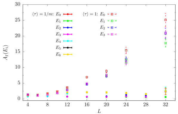
Figure 7: Continuum scaling of the integrated autocorrelations $A_{I}(E_{i})$ in HSPT for the cases $\langle\tau\rangle=1$ and $\langle\tau\rangle=1/m$. For $\langle\tau\rangle=1$ we show results only up to $O(g_{0}^{3})$, while for $\langle\tau\rangle=1/m$ they go up to $O(g_{0}^{6})$. The data is for $z=4$ and $c=0.2$. We measure the observables after each trajectory. The errors on the integrated autocorrelations were estimated using the $\Gamma$-method [43].

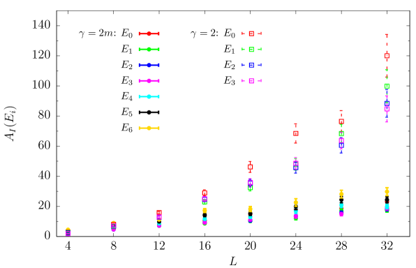
Figure 8: Continuum scaling of the integrated autocorrelations $A_{I}(E_{i})$ in KSPT for the cases $\gamma=2$ and $\gamma=2m$. For $\gamma=2$ we show results only up to $O(g_{0}^{3})$, while for $\gamma=2m$ they go up to $O(g_{0}^{6})$. The data is for $z=4$, $c=0.2$. The step-size is $\delta t=0.25$ and we measure the observables after each step. The errors on the integrated autocorrelations were estimated using the $\Gamma$-method [43].

For KSPT the results from free field theory [38] indicate that at the lowest order in perturbation theory the autocorrelations are expected to increase as $L^{2}$ as the continuum limit is approached if the parameter $\gamma$ is kept fixed. However, they increase only as $L$ if $\gamma\propto m$ (see also [36]). Hence $\gamma$ effectively plays the role of an inverse trajectory length for the algorithm [33]. In Figure 8 we report the results for $A_{I}(E_{i})$ for these two cases. In the first case we fixed $\gamma=2$ as $L\to\infty$, while in the second case we set $\gamma=2m$. We measured the observables after each step, and chose $z=4$ and $c=0.2$. Unlike the case of HSPT we chose a fixed step-size $\delta t=0.25$, and we kept this constant as $L\to\infty$. As we can see from the figure the two cases agree with the free field theory expectations for all the perturbative orders we investigated.

In conclusion, it seems that the free field theory expectations for autocorrelations of the HMD and Kramers algorithms apply up to relatively high perturbative orders in the corresponding NSPT implementations. Except for the case of KSPT at fixed $\gamma$ this is a non-trivial result in view of the non-renormalizability of the HMD and SMD equations [30, 36].

6.4 Continuum variance scaling

Having investigated the dependence of the continuum scaling of the integrated autocorrelations for different algorithmic parameter scalings, we next studied the corresponding scaling of the variances $\mathop{\rm Var}(E_{i})$. In Figure 9 we present results for the ratios $\mathop{\rm Var}(E_{i})/\mathop{\rm Var}(E_{0})$ with $i=1,2,3$ for HSPT, comparing the cases $\langle\tau\rangle=1$ and $\langle\tau\rangle=1/m$ as $L\to\infty$. For convenience the results are normalized by their values at $L=4$. As usual we chose $z=4$, $c=0.2$, and took $4\leq L\leq 32$ and $\delta t=2/L$. Recall that the lowest order variance $\mathop{\rm Var}(E_{0})$ is independent of the algorithmic parameters, namely $\langle\tau\rangle$ (or $\gamma$ below), and up to $O(1/L^{2})$ corrections is constant with $L$. Observe that upon setting $\langle\tau\rangle=1/m$ the variances $\mathop{\rm Var}(E_{i})$ with $i>1$ increase significantly as the continuum limit is approached. This effect is more pronounced as the perturbative order increases; on the other hand for $\langle\tau\rangle=1$ the variances for all the perturbative orders considered grow very slowly with $L$ and do not change significantly over the whole range of lattice sizes studied.

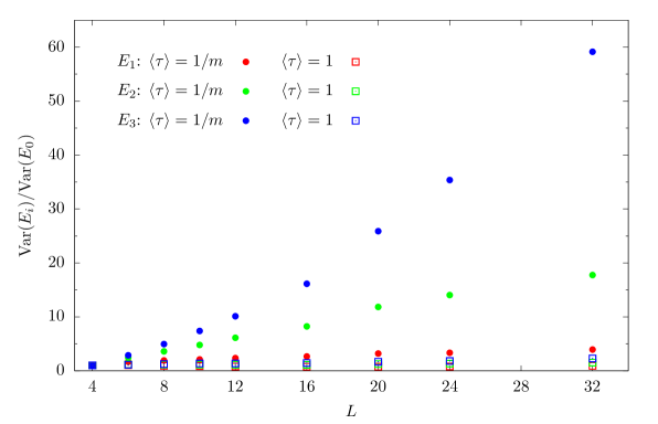
Figure 9: Continuum scaling of the ratios $\mathop{\rm Var}(E_{i})/\mathop{\rm Var}(E_{0})$ with $i=1,2,3$ for HSPT, for the cases $\langle\tau\rangle=1/m$ and $\langle\tau\rangle=1$. The case of $z=4$ and $c=0.2$ is shown, and the data are normalized at $L=4$.

In Figure 10 we plot the results for the ratios $\mathop{\rm Var}(E_{i})/\mathop{\rm Var}(E_{0})$ as obtained with KSPT. The two cases $\gamma=2m$ and $\gamma=2$ are shown. These results are very similar to those for HSPT: $\gamma=2m$ leads to larger variances than keeping $\gamma=2$ fixed, and these variances grow rapidly with perturbative order as the continuum limit is approached.

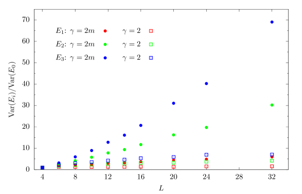
Figure 10: Continuum scaling of the ratios $\mathop{\rm Var}(E_{i})/\mathop{\rm Var}(E_{0})$ for $i=1,2,3$ for KSPT, for the cases $\gamma=2m$ and $\gamma=2$. The case of $z=4$ and $c=0.2$ is shown, and the data are normalized at $L=4$.

These results show that beyond the lowest perturbative order not only do the autocorrelations of observables computed using NSPT depend on the parameters of the algorithms but their variances do too. This is quite a different situation to the familiar case of non-perturbative computations.

6.5 Continuum cost scaling and parameter tuning: the case of KSPT

6.5.1 Continuum cost scaling

From the results of the previous subsections it is clear that the most cost-effective tuning of parameters for a NSPT simulation is not trivial to determine. For all cases considered decreasing autocorrelations occurs concomitantly with increasing variances; the optimal compromise between the two effects must be found.

The situation is clear if we look directly at the total error (6.45) rather than at autocorrelations and variances separately, and compare the two parameter scalings investigated above. For illustration we consider the case of KSPT; HSPT gives very similar results. In Figure 11 we compare the relative error $\Delta\mathcal{E}_{i}/\mathcal{E}_{i}$ with $i=0,1,2$ for the cases $\gamma=2$ and $\gamma=2m$. The number of configurations for the two parameter scalings is fixed to $N_{\mbox{\tiny config}}=10^{6}$ for all the lattice sizes $4\leq L\leq 20$. As usual the data is for $z=4$, $c=0.2$. We took $\delta t=2/L$ and adjusted the measurement frequency $\propto L$. As expected, setting $\gamma=2m$ is beneficial compared to having $\gamma=2$ at the lowest perturbative order (top panel of Figure 11). On the other hand, when considering higher perturbative orders the case $\gamma=2m$ seems to give comparable if not larger errors than fixing $\gamma=2$ as $L\to\infty$. Hence, for the range of lattice sizes and perturbative orders we investigated, the effect of having smaller autocorrelations for $\gamma=2m$ appears to be compensated if not overcome by the corresponding increase of the variances.

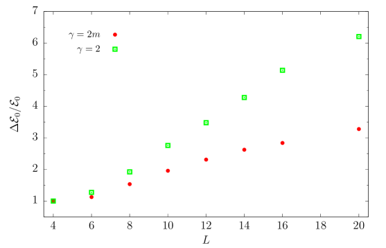
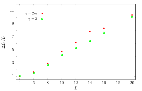
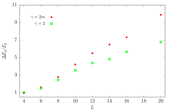
Figure 11: Relative errors $\Delta\mathcal{E}_{i}/\mathcal{E}_{i}$, $i=0,1,2$, as a function of $L$ for the two cases $\gamma=2$ and $\gamma=2m$. The data are normalized at $L=4$.

6.5.2 Parameter tuning

It appears clear that optimizing the performance of the algorithms requires finding the optimal value of $\langle\tau\rangle$ or $\gamma$ for given lattice parameters, given observables, and the perturbative orders of interest. Focusing on the case of KSPT again, in Figure 12 we plot for example the relative errors $\Delta\mathcal{E}_{i}/\mathcal{E}_{i}$ for $i=0,1,2$ as a function of $\gamma$ for different values of $L$. For each $L$ and perturbative order, the total number of configurations $N_{\mbox{\tiny config}}$ was kept constant as $\gamma$ was varied, and the results are normalized by their values at $\gamma=2$. As usual $z=4$, $c=0.2$, and $\delta t=2/L$.

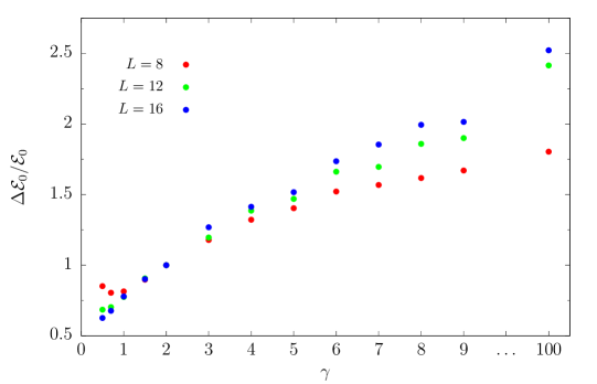
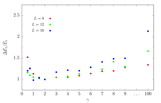
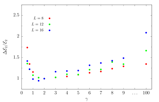
Figure 12: Relative errors $\Delta\mathcal{E}_{i}/\mathcal{E}_{i}$ with $i=0,1,2$ as a function of $\gamma$ for $L=8,12,16$. The data are normalized at $\gamma=2$, and the results for $\gamma=100$ are also shown. At this large value of $\gamma$ the algorithm is effectively integrating the Langevin equation.

At tree-level (top panel) increasing $\gamma$ leads to an increase of the relative error except at very small $\gamma$ values and small lattice size. This is expected because in this case the variance is independent of $\gamma$, while the autocorrelations increase with $\gamma$ until they saturate at some large enough value. In this regime the algorithm is effectively integrating the Langevin equation up to step-size errors. The situation for the higher perturbative orders $\mathcal{E}_{1}$ and $\mathcal{E}_{2}$ is quite different. For small $\gamma$ the errors fall rapidly as $\gamma$ is increased; as we expect the autocorrelations to be small in this case we interpret this as a rapid fall of the variances. For larger $\gamma$ values the errors increase only mildly compared to the situation at tree level. As at tree-level autocorrelations tend to grow with $\gamma$, but this effect is compensated by the variances decreasing as $\gamma$ is increased. In particular, we note that the Langevin limit $\gamma\to\infty$ is characterized by having the largest autocorrelations but the smallest variances. There is a region of $\gamma$ values for which the errors are minimized; in the example considered this does not appear to strongly depend on either the perturbative order or the lattice size. This is comforting as it allows us to tune $\gamma$ easily and to improve the efficiency of the algorithm relative to Langevin.

6.5.3 Cost comparison with LSPT

The results of the previous subsection show that a proper tuning of the parameter $\gamma$ increases the efficiency of KSPT over its Langevin limit, $\gamma\to\infty$. In the specific example considered, choosing a value of $\gamma\approx 2$ appears to be a good compromise for the different perturbative orders investigated, and it leads to a reduction of the statistical errors at fixed cost by a factor $\approx 2-2.5$ for $L=16$ as compared to $\gamma\to\infty$; this corresponds to a factor $\approx 4-6$ in the cost at fixed statistical precision.

It is interesting to consider a direct comparison between KSPT and LSPT. We note that in practice LSPT differs from KSPT at $\gamma=\infty$ only by the different integration scheme used to integrate the Langevin equation. Hence, this comparison permits us to quantify the benefits of using efficient higher-order symplectic integrators in conjunction with a proper tuning of $\gamma$.

To this end, we compared the computational cost for computing the coefficients ${\cal E}_{i}$, $i=0,\ldots 3$, to a specified statistical accuracy using KSPT with $\gamma=2$ and LSPT. We chose to carry out this comparison with $L=12$, $z=4$ and $c=0.2$. For $L=12$ the reduction in the cost for a given statistical precision compared to $\gamma\to\infty$ is a factor $2-3$ for ${\cal E}_{k}$, $k=1,2,3$, and a factor 6 for ${\cal E}_{0}$ (q.v., Figure 12).

In view of the results of §6.1, we chose $\delta t=0.5$ for KSPT as we expect step-size errors to be very small compared to the precision of this test (see below). Similarly, for LSPT we took $\varepsilon=0.01$, which corresponds to the smallest step-size considered in §6.1. At this value we also expect step-size errors to be small, and this is the most expensive of the simulations considered in the extrapolation $\varepsilon\to 0$. At each step we made measurements for both KSPT and LSPT, and considered a total of configurations $N_{\rm config}=4\times 10^{6}$ and $4\times 10^{7}$, respectively. The results are collected in Table 3.

	${\cal E}_{0}\times 10^{5}$	${\cal E}_{1}\times 10^{8}$	${\cal E}_{2}\times 10^{9}$	${\cal E}_{3}\times 10^{10}$
LSPT	$2.2367(37)$	$-4.86(13)$	$2.352(54)$	$-1.599(40)$
KSPT	$2.2347(22)$	$-4.74(12)$	$2.223(49)$	$-1.517(35)$
LPT	$2.2347$	$-4.76$	$2.270$	$-$

Table 3: Results for ${\cal E}_{i}$, $i=0,\ldots 3$ for $L=12$, $z=4$, $c=0.2$ as obtained using KSPT with $\gamma=2$ and LSPT. We chose $\delta t=0.5$ for KSPT and $\varepsilon=0.01$ for LSPT, and measured at each step. The total number of configurations generated with the two algorithms is $N_{\rm config}=4\times 10^{6}$ and $4\times 10^{7}$ for KSPT and LSPT, respectively. The analytic perturbative results (LPT) for ${\cal E}_{0}$, ${\cal E}_{1}$, and ${\cal E}_{2}$ are also given for comparison.

The KSPT and LSPT results are statistically consistent with each other and with the closed-form perturbative results (LPT) where these are available. KSPT and LSPT have approximately the same statistical errors with the numbers of configurations generated. The computer time used for updating a $12^{4}$ lattice on a single core of an Intel Xeon E5-2630 Processor (2.4 GHz) is $0.21s$ for LSPT and $0.42s$ for KSPT: this is just the expected ratio of costs between the RK2 and OMF4 integrators, with the observation that this cost is dominated by the force computation.

Thus, after rescaling $N_{\rm config}$ to have equal statistical errors, it becomes apparent that KSPT is $\approx 5-7$ times more cost effective than LSPT is in reaching a given statistical precision on the higher-order coefficients ${\cal E}_{k}$, $k=1,2,3$, and roughly 14 times more cost effective for ${\cal E}_{0}$. As KSPT at fixed $\gamma$ and LSPT have the same continuum scaling behavior in terms of variances and autocorrelations, one may expect a similar gain as $L\to\infty$. Indeed, as shown in Figure 12, the gain in the statistical errors appears to become larger for the higher-order fields at larger $L$; if one scales the gain in cost accordingly this increases to a factor $\approx 9-10$ for ${\cal E}_{1}$ and ${\cal E}_{2}$. Furthermore, as the continuum limit is approached, it is advisable to reduce the step-size so as to keep systematic effects under control, and here again higher-order integrators are more cost effective.

7 Conclusions

NSPT is a powerful technique that permits automation of high order perturbative computations on the lattice. As well as providing perturbative lattice estimates of quantities of interest these methods are interesting for extracting continuum perturbation theory results in cases where these are difficult or unfeasible to obtain with continuum perturbative methods. However, to this end one needs efficient NSPT algorithms in order to be able to obtain precise results with both systematic and statistical errors under control. In particular, such results are desirable for a collection of lattice resolutions close to the continuum limit so that reliable continuum extrapolations may be performed.

In this work we investigated some new formulations of NSPT beyond LSPT, with the goal of finding more cost-effective algorithms. The first of these techniques is the recently proposed ISPT [12]. The first manifest advantage of this method over standard LSPT is that the results obtained are exact within statistical errors. Secondly, the stochastic field representing the theory to some given order in the couplings is constructed directly from a set of Gaussian random fields, which are easy to generate. Despite these attractive features this algorithm has severe limitations beyond the lowest perturbative orders. First, similarly to conventional diagrammatic perturbation theory, the number of diagrams to be computed grows very rapidly with the perturbative order. While the cost of evaluating the diagrams is essentially proportional to the system size, their number increases exponentially as the perturbative order is increased. Most importantly, as shown by the present study, as the continuum limit is approached the statistical variance of perturbative coefficients computed using ISPT grows with increasing powers of $L$ as the perturbative order is increased. Consequently it appears difficult to extract precise high-order results close to the continuum limit using this technique. While the exact details of our investigation certainly depend on the theory we considered, our conclusions are not specific to $\varphi^{4}$-theory. This has been confirmed by a recent study in the pure $\mathop{\rm SU}(3)$ Yang–Mills theory [44], where the nature of the divergences of the variances was also elucidated. In summary, the utility of this technique may be limited to a few low perturbative orders, which can nonetheless be of interest for some particularly difficult problems.

Although they are not exact the other NSPT algorithms we considered, where the stochastic fields representing the theory are generated by a Markov chain (or equivalently a discrete stochastic process), in general have a significantly better continuum cost scaling than ISPT. In particular, apart from the standard LSPT, we considered NSPT based on GHMD algorithms; specifically the HMD and Kramers algorithms. With respect to the Langevin implementation, these allow for a much more accurate discretization of the relevant equations. This is so because very efficient high-order symplectic integrators can be employed for the numerical integration of the MD equations. With such integrators the magnitude of the systematic errors is drastically reduced for a given number of force computations, and in practice one can run these algorithms with a small enough step-size that step-size extrapolations can be avoided.

As opposed to LSPT, HSPT and KSPT have tunable parameters, the average trajectory length $\langle\tau\rangle$ and the amount of partial momentum refreshment $\gamma$ respectively, which may be adjusted so as to optimize their efficiency. However, beyond the lowest perturbative order finding the most cost-effective tuning of these parameters is not immediately obvious, in particular because their optimal continuum scaling is not trivial. The situation is complicated by the fact that, unlike the more familiar non-perturbative simulations, not only do the autocorrelations of the perturbative coefficients computed in NSPT depend on the parameters of the chosen algorithm, but so do their variances. The general trend we observed is that when an algorithm is tuned to have small autocorrelations, the corresponding variances tend to increase, and therefore a trade-off between these two effects must be found. Moreover, except in the Langevin limit of these algorithms, analytic understanding of the continuum scaling of both autocorrelations and variances is missing.

Our analysis indicates that the behavior of the autocorrelations of the high order fields with respect to the algorithmic parameters is the same as in the free field case. The behaviour of the variances is not easily predicted, and it seems to be different for different perturbative orders. A consequence of this is the fact that the optimal parameter scaling suggested by free field theory is not optimal when higher perturbative orders are considered. In our study we did not observe a significant difference in the cost with respect to the Langevin scaling of the algorithms (§6.5.1). Finding the optimal parameter scaling might thus be difficult, as it probably depends on the details of the calculation considered, i.e., the observables, the perturbative orders, and range of lattice sizes of interest.

Nonetheless, when investigating the dependence of the errors in KSPT as a function of $\gamma$ (§6.5.2) we found that for $\gamma\approx 2$ the algorithm is significantly better than in its Langevin limit $\gamma\to\infty$, particularly so for large $L$. For example, at $L=16$ an improvement by a factor $\approx 4-6$ in the cost of obtaining a given statistical precision was observed, depending on the order. This was possible since for the observables studied the optimal value of $\gamma$ did not seem to depend much on either $L$ or the perturbative order. When we compared KSPT at $\gamma=2$ with LSPT (§6.5.3), the use of efficient high-order integrators turned out to be beneficial in keeping systematic errors under control in a more cost effective way than using lower-order Runge-Kutta integrators, keeping this value of $\gamma$ fixed as $L\to\infty$ improves significantly the efficiency of the algorithm over LSPT. Indeed, although the scaling behaviour of the statistical errors may be the same one profits from a significantly smaller prefactor, as well as the better scaling (and prefactor) of the high-order symplectic integrators in controlling step-size errors.

We also observe that HSPT and KSPT have similar performance: for $\langle\tau\rangle=C/\gamma$ with $C=O(1)$ the two algorithms have comparable autocorrelations in molecular dynamics units, and comparable variances.

In conclusion, the novel NSPT methods presented here offer a simple and natural development from the standard Langevin-based algorithms. In particular, we have provided evidence that they can significantly improve on previous methods hence allowing more precise results. Of course, a natural follow-up of our study is to consider the application of these techniques to a realistic problem in order to determine whether the improvement provided by HSPT or KSPT is significant in practice. These methods have been used and are under further development for the more interesting case of gauge theories [45, 46].

Appendix A Renormalization procedure

A.1 Coupling renormalization

In regularized $\phi^{4}$ theory we may compute an observable ${\cal O}$ as a perturbative expansion in the bare coupling $g_{0}$. However, in order to take the continuum limit of its expectation value, it is first of all necessary to express this perturbative series in terms of a renormalized coupling $g$. Of course, at finite lattice cutoff, the two are entirely equivalent as formal expansions and may readily be transformed into each other.

Suppose we have computed the perturbative expansion of the renormalized coupling $g$ as a power series in the bare coupling $g_{0}$,

$$g=g_{0}+\sum_{k\geq 2}c_{k}g_{0}^{k}.$$ (A.47)

We may then revert the expansion of $g$ in terms of $g_{0}$ by writing (A.47) as

$$g_{0}=g-\sum_{k\geq 2}c_{k}g_{0}^{k},$$ (A.48)

and then recursively substituting (A.48) into itself to obtain

$$g_{0} =g-\sum_{k\geq 2}c_{k}\Bigl{(}g-\sum_{\ell\geq 2}c_{\ell}g_{0}^{\ell}\Bigr{)}^{k}$$

$$=g-c_{2}g^{2}+(2c_{2}^{2}-c_{3})g^{3}+(-5c_{2}^{3}+5c_{2}c_{3}-c_{4})g^{4}$$

$$\qquad+(14c_{2}^{4}-21c_{2}^{2}c_{3}+6c_{2}c_{4}+3c_{3}^{2}-c_{5})g^{5}$$

$$\qquad+(-42c_{2}^{5}+84c_{2}^{3}c_{3}-28c_{2}^{2}c_{4}-28c_{2}c_{3}^{2}+7c_{2}c_{5}+7c_{3}c_{4}-c_{6})g^{6}+\cdots,$$ (A.49)

noting that $O(g_{0}^{N})=O(g^{N})$.

Suppose that we have also computed the expansion of some operator of interest ${\cal O}$ in powers of $g_{0}$

$${\cal O}=\sum_{k\geq 0}{\cal O}_{k}g_{0}^{k},$$ (A.50)

Then by substituting (A.49) into (A.50) we obtain an expression for the expansion of ${\cal O}$ in powers of $g$:

$${\cal O} ={\cal O}_{0}+{\cal O}_{1}g+(-c_{2}{\cal O}_{1}+{\cal O}_{2})g^{2}+\bigl{(}(2c_{2}^{2}-c_{3}){\cal O}_{1}-2c_{2}{\cal O}_{2}+{\cal O}_{3}\bigr{)}g^{3}$$

$$\qquad+\bigl{(}(-5c_{2}^{3}+5c_{2}c_{3}-c_{4}){\cal O}_{1}+(5c_{2}^{2}-2c_{3}){\cal O}_{2}-3c_{2}{\cal O}_{3}+{\cal O}_{4}\bigr{)}g^{4}$$

$$\qquad+\bigl{(}(14c_{2}^{4}-21c_{2}^{2}c_{3}+6c_{2}c_{4}+3c_{3}^{2}-c_{5}){\cal O}_{1}+(-14c_{2}^{3}+12c_{2}c_{3}-2c_{4}){\cal O}_{2}$$

$$\qquad\qquad+(9c_{2}^{2}-3c_{3}){\cal O}_{3}-4c_{2}{\cal O}_{4}+{\cal O}_{5}\bigr{)}g^{5}$$

$$\qquad+\bigl{(}(-42c_{2}^{5}+84c_{2}^{3}c_{3}-28c_{2}^{2}c_{4}-28c_{2}c_{3}^{2}+7c_{2}c_{5}+7c_{3}c_{4}-c_{6}){\cal O}_{1}$$

$$\qquad\qquad+(42c_{2}^{4}-56c_{2}^{2}c_{3}+14c_{2}c_{4}+7c_{3}^{2}-2c_{5}){\cal O}_{2}$$

$$\qquad\qquad+(-28c_{2}^{3}+21c_{2}c_{3}-3c_{4}){\cal O}_{3}+(14c_{2}^{2}-4c_{3}){\cal O}_{4}-5c_{2}{\cal O}_{5}+{\cal O}_{6}\bigr{)}g^{6}+\cdots$$

For the numerical computation of the perturbative expansion of ${\cal O}$ we are therefore free to consider an expansion in powers of $g_{0}$ as this is entirely equivalent — as formal power series — to expansion in powers of $g$.

A.2 Mass renormalization

The stochastic field $\phi$ is considered to be of the form

$$\phi(x)=\sum_{k,l\geq 0}\phi_{k,\ell}(x)g_{0}^{k}(\delta m^{2})^{\ell}$$ (A.51)

where $g_{0}$ is the bare coupling and $\delta m^{2}$ is the mass counterterm. Once the table of numbers $\phi_{k,\ell}$ has been computed, the expectation value $\langle\cdots\rangle_{\eta}$ of functions of these quantities may be estimated, but they must be fitted to the renormalization conditions in order to compute physical quantities. Here we shall present algebraic expressions for the formal power series manipulation in order to explain the renormalization procedure; in actual computations we automated these formal manipulations using the numerical values of the coefficients.

The renormalization condition (2.7) that defines $m^{2}$ can be rewritten as

$$m^{2}=\hat{p}_{*}^{2}\frac{\chi_{2}^{*}}{\chi_{2}-\chi_{2}^{*}}.$$

Therefore, since we can calculate $\chi_{2}$ and $\chi_{2}^{*}$ as power series in both $g_{0}$ and $\delta m^{2}$

$$\chi_{2} =\Bigl{\langle}\tilde{\phi}_{0,0}(0)^{2}\Bigr{\rangle}+2\Bigl{\langle}\tilde{\phi}_{0,0}(0)\tilde{\phi}_{0,1}(0)\Bigr{\rangle}\delta m^{2}+\Bigl{\langle}2\tilde{\phi}_{0,0}(0)\tilde{\phi}_{0,2}(0)+\tilde{\phi}_{0,1}(0)^{2}\Bigr{\rangle}\delta m^{4}$$

$$\qquad+2\Bigl{\langle}\tilde{\phi}_{0,0}(0)\tilde{\phi}_{0,3}(0)+\tilde{\phi}_{0,1}(0)\tilde{\phi}_{0,2}(0)\Bigr{\rangle}\delta m^{6}$$

$$\quad+2\biggl{(}\Bigl{\langle}\tilde{\phi}_{0,0}(0)\tilde{\phi}_{1,0}(0)\Bigr{\rangle}+\Bigl{\langle}\tilde{\phi}_{0,0}(0)\tilde{\phi}_{1,1}(0)+\tilde{\phi}_{1,0}(0)\tilde{\phi}_{0,1}(0)\Bigr{\rangle}\delta m^{2}$$

$$\qquad+\Bigl{\langle}\tilde{\phi}_{0,0}(0)\tilde{\phi}_{1,2}(0)+\tilde{\phi}_{1,0}(0)\tilde{\phi}_{0,2}(0)+\tilde{\phi}_{0,1}(0)\tilde{\phi}_{1,1}(0)\Bigr{\rangle}\delta m^{4}\biggr{)}g_{0}$$

$$\quad+\biggl{(}\Bigl{\langle}2\tilde{\phi}_{0,0}(0)\tilde{\phi}_{2,0}(0)+\tilde{\phi}_{1,0}(0)^{2}\Bigr{\rangle}$$

$$\qquad+2\Bigl{\langle}\tilde{\phi}_{0,0}(0)\tilde{\phi}_{2,1}(0)+\tilde{\phi}_{1,0}(0)\tilde{\phi}_{1,1}(0)+\tilde{\phi}_{0,1}(0)\tilde{\phi}_{2,0}(0)\Bigr{\rangle}\delta m^{2}\biggr{)}g_{0}^{2}$$

$$\quad+2\Bigl{\langle}\tilde{\phi}_{0,0}(0)\tilde{\phi}_{3,0}(0)+\tilde{\phi}_{1,0}(0)\tilde{\phi}_{2,0}(0)\Bigr{\rangle}g_{0}^{3}+O(g_{0}^{4})$$

$$\chi_{2}^{*} =\Bigl{\langle}\tilde{\phi}_{0,0}(p_{*})\tilde{\phi}_{0,0}(-p_{*})\Bigr{\rangle}+\Bigl{\langle}\tilde{\phi}_{0,0}(p_{*})\tilde{\phi}_{0,1}(-p_{*})+\tilde{\phi}_{0,0}(-p_{*})\tilde{\phi}_{0,1}(p_{*})\Bigr{\rangle}\delta m^{2}$$

$$\qquad+\Bigl{\langle}\tilde{\phi}_{0,0}(p_{*})\tilde{\phi}_{0,2}(-p_{*})+\tilde{\phi}_{0,1}(p_{*})\tilde{\phi}_{0,1}(-p_{*})+\tilde{\phi}_{0,0}(-p_{*})\tilde{\phi}_{0,2}(p_{*})\Bigr{\rangle}\delta m^{4}$$

$$\qquad+\Bigl{\langle}\tilde{\phi}_{0,0}(p_{*})\tilde{\phi}_{0,3}(-p_{*})+\tilde{\phi}_{0,1}(p_{*})\tilde{\phi}_{0,2}(-p_{*})$$

$$\qquad\quad+\tilde{\phi}_{0,2}(p_{*})\tilde{\phi}_{0,1}(-p_{*})+\tilde{\phi}_{0,0}(-p_{*})\tilde{\phi}_{0,3}(p_{*})\Bigr{\rangle}\delta m^{6}$$

$$\quad+\biggl{(}\Bigl{\langle}\tilde{\phi}_{0,0}(p_{*})\tilde{\phi}_{1,0}(-p_{*})+\tilde{\phi}_{0,0}(-p_{*})\tilde{\phi}_{1,0}(p_{*})\Bigr{\rangle}$$

$$\qquad+\Bigl{\langle}\tilde{\phi}_{0,0}(p_{*})\tilde{\phi}_{1,1}(-p_{*})+\tilde{\phi}_{1,0}(p_{*})\tilde{\phi}_{0,1}(-p_{*})$$

$$\qquad\quad+\tilde{\phi}_{0,1}(p_{*})\tilde{\phi}_{1,0}(-p_{*})+\tilde{\phi}_{0,0}(-p_{*})\tilde{\phi}_{1,1}(p_{*})\Bigr{\rangle}\delta m^{2}$$

$$\qquad+\Bigl{\langle}\tilde{\phi}_{0,0}(p_{*})\tilde{\phi}_{1,2}(-p_{*})+\tilde{\phi}_{1,0}(p_{*})\tilde{\phi}_{0,2}(-p_{*})$$

$$\qquad\quad+\tilde{\phi}_{0,1}(p_{*})\tilde{\phi}_{1,1}(-p_{*})+\tilde{\phi}_{1,1}(p_{*})\tilde{\phi}_{0,1}(-p_{*})$$

$$\qquad\quad+\tilde{\phi}_{0,2}(p_{*})\tilde{\phi}_{1,0}(-p_{*})+\tilde{\phi}_{0,0}(-p_{*})\tilde{\phi}_{1,2}(p_{*})\Bigr{\rangle}\delta m^{4}\biggr{)}g_{0}$$

$$\quad+\biggl{(}\Bigl{\langle}\tilde{\phi}_{0,0}(p_{*})\tilde{\phi}_{2,0}(-p_{*})+\tilde{\phi}_{1,0}(p_{*})\tilde{\phi}_{1,0}(-p_{*})+\tilde{\phi}_{0,0}(-p_{*})\tilde{\phi}_{2,0}(p_{*})\Bigr{\rangle}$$

$$\qquad+\Bigl{\langle}\tilde{\phi}_{0,0}(p_{*})\tilde{\phi}_{2,1}(-p_{*})+\tilde{\phi}_{1,0}(p_{*})\tilde{\phi}_{1,1}(-p_{*})$$

$$\qquad\quad+\tilde{\phi}_{0,1}(p_{*})\tilde{\phi}_{2,0}(-p_{*})+\tilde{\phi}_{2,0}(p_{*})\tilde{\phi}_{0,1}(-p_{*})$$

$$\qquad\quad+\tilde{\phi}_{1,1}(p_{*})\tilde{\phi}_{1,0}(-p_{*})+\tilde{\phi}_{0,0}(-p_{*})\tilde{\phi}_{2,1}(p_{*})\Bigr{\rangle}\delta m^{2}\biggr{)}g_{0}^{2}$$

$$\quad+\biggl{(}\Bigl{\langle}\tilde{\phi}_{0,0}(p_{*})\tilde{\phi}_{3,0}(-p_{*})+\tilde{\phi}_{1,0}(p_{*})\tilde{\phi}_{2,0}(-p_{*})$$

$$\qquad+\tilde{\phi}_{2,0}(p_{*})\tilde{\phi}_{1,0}(-p_{*})+\tilde{\phi}_{0,0}(-p_{*})\tilde{\phi}_{3,0}(p_{*})\Bigr{\rangle}\biggr{)}g_{0}^{3}+O(g_{0}^{4})$$

where we defined the Fourier transform of the coefficient fields as,

$$\tilde{\phi}_{k,l}(p)=\frac{1}{L^{2}}\sum_{x\in\Omega}e^{-ipx}\phi_{k,l}(x),\quad p\in\tilde{\Omega},$$

we can multiply and invert $\chi$ and $\chi^{*}$ to compute $m^{2}$ as power series in $g_{0}$ and $\delta m^{2}$

$$m^{2}=\sum_{k,\ell\geq 0}a_{k,\ell}\,g_{0}^{k}(\delta m^{2})^{\ell}$$ (A.52)

where the coefficients $a_{k,\ell}$ are

$$a_{0,0} =\frac{\Bigl{\langle}\tilde{\phi}_{0,0}(p_{*})\tilde{\phi}_{0,0}(-p_{*})\Bigr{\rangle}}{\Bigl{\langle}\tilde{\phi}_{0,0}(0)^{2}-\tilde{\phi}_{0,0}(p_{*})\tilde{\phi}_{0,0}(-p_{*})\Bigr{\rangle}}\,\hat{p}_{*}^{2},$$

$$a_{1,0} =-\frac{\begin{array}[]{l}2\Bigl{\langle}\tilde{\phi}_{0,0}(0)\tilde{\phi}_{1,0}(0)\Bigr{\rangle}\Bigl{\langle}\tilde{\phi}_{0,0}(p_{*})\tilde{\phi}_{0,0}(-p_{*})\Bigr{\rangle}\\ \qquad\qquad-\Bigl{\langle}\tilde{\phi}_{0,0}(0)^{2}\Bigr{\rangle}\Bigl{\langle}\tilde{\phi}_{0,0}(p_{*})\tilde{\phi}_{1,0}(-p_{*})+\tilde{\phi}_{0,0}(-p_{*})\tilde{\phi}_{1,0}(p_{*})\Bigr{\rangle}\end{array}}{\Bigl{\langle}\tilde{\phi}_{0,0}(0)^{2}-\tilde{\phi}_{0,0}(p_{*})\tilde{\phi}_{0,0}(-p_{*})\Bigr{\rangle}^{2}}\,\hat{p}_{*}^{2},$$

$$a_{0,1} =-\frac{\begin{array}[]{l}2\Bigl{\langle}\tilde{\phi}_{0,0}(0)\tilde{\phi}_{0,1}(0)\Bigr{\rangle}\Bigl{\langle}\tilde{\phi}_{0,0}(p_{*})\tilde{\phi}_{0,0}(-p_{*})\Bigr{\rangle}\\ \qquad\qquad-\Bigl{\langle}\tilde{\phi}_{0,0}(0)^{2}\Bigr{\rangle}\Bigl{\langle}\tilde{\phi}_{0,0}(p_{*})\tilde{\phi}_{0,1}(-p_{*})+\tilde{\phi}_{0,0}(-p_{*})\tilde{\phi}_{0,1}(p_{*})\Bigr{\rangle}\end{array}}{\Bigl{\langle}\tilde{\phi}_{0,0}(0)^{2}-\tilde{\phi}_{0,0}(p_{*})\tilde{\phi}_{0,0}(-p_{*})\Bigr{\rangle}^{2}}\,\hat{p}_{*}^{2},$$

and so forth. By construction $a_{0,0}=m^{2}$, so at lowest order in $g_{0}$ the mass $m$ is the mass that enters the scalar propagator (3.24). Having determined the coefficient $a_{k,\ell}$ in (A.52) we can now determine the coefficients $m_{k}^{2}$ of the expansion

$$\delta m^{2}=\sum_{k\geq 1}m^{2}_{k}\,g_{0}^{k}$$

by imposing the relation (A.52) order by order in $g_{0}$, thus obtaining

$$m_{1}^{2} =-\frac{a_{1,0}}{a_{0,1}},$$

$$m_{2}^{2} =-\frac{a_{2,0}+a_{1,1}m_{1}^{2}+a_{0,2}m_{1}^{4}}{a_{0,1}},$$

$$m_{3}^{2} =-\frac{a_{3,0}+a_{2,1}m_{1}^{2}+2a_{0,2}m_{1}^{2}m_{2}^{2}+a_{1,2}m_{1}^{4}+a_{1,1}m_{2}^{2}+a_{0,3}m_{1}^{6}}{a_{0,1}},$$

$$m_{4}^{2} =-\frac{\begin{array}[]{l}a_{4,0}+a_{3,1}m_{1}^{2}+a_{2,1}m_{2}^{2}+a_{1,1}m_{3}^{2}+a_{2,2}m_{1}^{4}+2a_{1,2}m_{1}^{2}m_{2}^{2}\\ \qquad\qquad+a_{0,2}m_{2}^{4}+2a_{0,2}m_{1}^{2}m_{3}^{2}+a_{1,3}m_{1}^{6}+3a_{0,3}m_{1}^{4}m_{2}^{2}+a_{0,4}m_{1}^{8}\end{array}}{a_{0,1}},$$

$$\vdots$$

Once $\delta m^{2}$ is determined, the field $\phi$ and any other observable previously computed as a series in $\delta m^{2}$ and $g_{0}$ can be reduced to a series in $g_{0}$ alone.

A.3 Wavefunction renormalization

The renormalization of a generic correlation function by the wavefunction renormalization, or any multiplicative renormalization factor, does not present any additional difficulty. We may compute $Z$ as a power series in $g_{0}$ and $\delta m^{2}$ from the renormalization condition (2.9),

$$Z=m^{2}\chi=\sum_{k,\ell\geq 0}Z_{k,\ell}\,g_{0}^{k}(\delta m^{2})^{\ell},$$

where

$$Z_{0,0} =a_{0,0}\Bigl{\langle}\tilde{\phi}_{0,0}(0)^{2}\Bigr{\rangle}$$

$$Z_{1,0} =a_{1,0}\Bigl{\langle}\tilde{\phi}_{0,0}(0)^{2}\Bigr{\rangle}+2a_{0,0}\Bigl{\langle}\tilde{\phi}_{1,0}(0)\tilde{\phi}_{0,0}(0)\Bigr{\rangle}$$

$$Z_{0,1} =a_{0,1}\Bigl{\langle}\tilde{\phi}_{0,0}(0)^{2}\Bigr{\rangle}+2a_{0,0}\Bigl{\langle}\tilde{\phi}_{0,0}(0)\tilde{\phi}_{0,1}(0)\Bigr{\rangle}$$

$$Z_{2,0} =2a_{0,0}\Bigl{\langle}\tilde{\phi}_{0,0}(0)\tilde{\phi}_{2,0}(0)\Bigr{\rangle}+a_{0,0}\Bigl{\langle}\tilde{\phi}_{1,0}(0)^{2})\Bigr{\rangle}$$

$$\qquad+2a_{1,0}\Bigl{\langle}\tilde{\phi}_{0,0}(0)\tilde{\phi}_{1,0}(0)\Bigr{\rangle}+a_{2,0}\Bigl{\langle}\tilde{\phi}_{0,0}(0)^{2})\Bigr{\rangle}$$

$$Z_{1,1} =2a_{0,0}\Bigl{\langle}\tilde{\phi}_{0,0}(0)\tilde{\phi}_{1,1}(0)\Bigr{\rangle}+2a_{0,0}\Bigl{\langle}\tilde{\phi}_{1,0}(0)\tilde{\phi}_{0,1}(0)\Bigr{\rangle}$$

$$\qquad+2a_{0,1}\Bigl{\langle}\tilde{\phi}_{0,0}(0)\tilde{\phi}_{1,0}(0)\Bigr{\rangle}+2a_{1,0}\Bigl{\langle}\tilde{\phi}_{0,0}(0)\tilde{\phi}_{0,1}(0)\Bigr{\rangle}+a_{1,1}\Bigl{\langle}\tilde{\phi}_{0,0}(0)^{2}\Bigr{\rangle}$$

$$Z_{0,2} =2a_{0,0}\Bigl{\langle}\tilde{\phi}_{0,0}(0)\tilde{\phi}_{0,2}(0)\Bigr{\rangle}+a_{0,0}\Bigl{\langle}\tilde{\phi}_{0,1}(0)^{2}\Bigr{\rangle}$$

$$\qquad+2a_{0,1}\Bigl{\langle}\tilde{\phi}_{0,0}(0)\tilde{\phi}_{0,1}(0)\Bigr{\rangle}+a_{0,2}\Bigl{\langle}\tilde{\phi}_{0,0}(0)^{2}\Bigr{\rangle},$$

and so forth. We can now compute a renormalized correlation function as a power series in $g_{0}$ and the renormalized mass $m$ as

$$Z^{n/2}\bigl{\langle}\phi(x_{1})\cdots\phi(x_{n})\bigr{\rangle}=\bigg{(}\sum_{k,\ell\geq 0}Z_{k,\ell}\,g_{0}^{k}(\delta m^{2})^{\ell}\bigg{)}^{n/2}$$

$$\qquad\times\left\langle\sum_{k_{1},\ell_{1}\geq 0}\phi_{k_{1},\ell_{1}}(x_{1})g_{0}^{k_{1}}(\delta m^{2})^{\ell_{1}}\>\cdots\sum_{k_{n},\ell_{n}\geq 0}\phi_{k_{n},\ell_{n}}(x_{n})g_{0}^{k_{n}}(\delta m^{2})^{\ell_{n}}\right\rangle$$

$$=\bigg{(}\sum_{k,l\geq 0}Z_{k,\ell}\,g_{0}^{k}\Big{(}\sum_{j\geq 1}m_{j}^{2}\,g_{0}^{j}\Big{)}^{\ell}\bigg{)}^{n/2}$$

$$\qquad\times\left\langle\sum_{k_{1},\ell_{1}\geq 0}\phi_{k_{1},\ell_{1}}(x_{1})g_{0}^{k_{1}}\Big{(}\sum_{j_{1}\geq 1}m_{j_{1}}^{2}\,g_{0}^{j_{1}}\Big{)}^{\ell_{1}}\cdots\sum_{k_{n},\ell_{n}\geq 0}\phi_{k_{n},\ell_{n}}(x_{n})g_{0}^{k_{n}}\Big{(}\sum_{j_{n}\geq 1}m_{j_{n}}^{2}\,g_{0}^{j_{n}}\Big{)}^{\ell_{n}}\right\rangle.$$

This expansion in the bare coupling $g_{0}$ can be replaced by one in the renormalized coupling $g$ as explained in §A.1, and the correlation function is then properly renormalized.

References

- [1] H. J. Rothe, Lattice gauge theories: An Introduction, World Sci. Lect. Notes Phys. 43 (1992) 1–381. [World Sci. Lect. Notes Phys. 82 (2012) 1].
- [2] I. Montvay and G. Munster, Quantum fields on a lattice. Cambridge University Press, 1997.
- [3] S. Capitani, Lattice perturbation theory, Phys. Rept. 382 (2003) 113–302.
- [4] F. Di Renzo, G. Marchesini, P. Marenzoni, and E. Onofri, Lattice perturbation theory on the computer, Nucl. Phys. Proc. Suppl. 34 (1994) 795–798.
- [5] F. Di Renzo, E. Onofri, G. Marchesini, and P. Marenzoni, Four loop result in SU(3) lattice gauge theory by a stochastic method: lattice correction to the condensate, Nucl. Phys. B426 (1994) 675–685.
- [6] F. Di Renzo and L. Scorzato, Numerical stochastic perturbation theory for full QCD, JHEP 0410 (2004) 073.
- [7] M. Brambilla, M. Dalla Brida, D. Hesse, F. Di Renzo, and S. Sint, Numerical Stochastic Perturbation Theory for Schrödinger Functional schemes, PoS LATTICE2013 (2013) 325.
- [8] M. Dalla Brida and D. Hesse, Numerical Stochastic Perturbation Theory and the Gradient Flow, PoS LATTICE2013 (2014) 326.
- [9] G. S. Bali, C. Bauer, A. Pineda, and C. Torrero, Perturbative expansion of the energy of static sources at large orders in four-dimensional SU(3) gauge theory, Phys. Rev. D87 (2013) 094517.
- [10] G. Parisi and Y. Wu, Perturbation Theory Without Gauge Fixing, Sci. Sin. 24 (1981) 483.
- [11] P. H. Damgaard and H. Hüffel, Stochastic Quantization, Phys. Rept. 152 (1987) 227.
- [12] M. Lüscher, Instantaneous stochastic perturbation theory, JHEP 04 (2015) 142.
- [13] M. Dalla Brida, M. Garofalo, and A. D. Kennedy, Numerical Stochastic Perturbation Theory and Gradient Flow in Theory, PoS LATTICE2015 (2015) 309.
- [14] P. Weisz and U. Wolff, Triviality of theory: small volume expansion and new data, Nucl. Phys. B846 (2011) 316–337.
- [15] M. Lüscher, Properties and uses of the Wilson flow in lattice QCD, JHEP 08 (2010) 071. [Erratum: JHEP 03 (2014) 092].
- [16] M. Lüscher and P. Weisz, Perturbative analysis of the gradient flow in non-abelian gauge theories, JHEP 02 (2011) 051.
- [17] C. Monahan and K. Orginos, Locally smeared operator product expansions in scalar field theory, Phys. Rev. D91 (2015), no. 7 074513.
- [18] C. Monahan, The gradient flow in simple field theories, PoS LATTICE2015 (2015) 052.
- [19] Z. Fodor, K. Holland, J. Kuti, D. Nogradi, and C. H. Wong, The Yang-Mills gradient flow in finite volume, JHEP 11 (2012) 007.
- [20] http://luscher.web.cern.ch/luscher/ISPT/.
- [21] M. Frigo and S. G. Johnson, The Design and Implementation of FFTW3, Proceedings of the IEEE 93 (2005), no. 2 216–231. Special issue on “Program Generation, Optimization, and Platform Adaptation”.
- [22] E. Floratos and J. Iliopoulos, Equivalence of Stochastic and Canonical Quantization in Perturbation Theory, Nucl. Phys. B214 (1983) 392.
- [23] J. Zinn-Justin, Renormalization and Stochastic Quantization, Nucl. Phys. B275 (1986) 135.
- [24] J. Zinn-Justin and D. Zwanziger, Ward Identities for the Stochastic Quantization of Gauge Fields, Nucl. Phys. B295 (1988) 297.
- [25] G. G. Batrouni, G. R. Katz, A. S. Kronfeld, G. P. Lepage, B. Svetitsky, and K. G. Wilson, Langevin Simulations of Lattice Field Theories, Phys. Rev. D32 (1985) 2736.
- [26] A. S. Kronfeld, Dynamics of Langevin simulations, Prog. Theor. Phys. Suppl. 111 (1993) 293–312.
- [27] J. Zinn-Justin, Quantum field theory and critical phenomena, International Series of Monographs on Physics (2002).
- [28] G. Aarts and F. A. James, Complex Langevin dynamics in the SU(3) spin model at nonzero chemical potential revisited, JHEP 01 (2012) 118.
- [29] L. Baulieu and D. Zwanziger, QCD(4) from a five-dimensional point of view, Nucl. Phys. B581 (2000) 604–640.
- [30] M. Lüscher and S. Schaefer, Non-renormalizability of the HMC algorithm, JHEP 04 (2011) 104.
- [31] M. Lüscher, Statistical errors in stochastic perturbation theory, notes available at http://luscher.web.cern.ch/luscher/notes/enspt.pdf (2015).
- [32] A. M. Horowitz, Stochastic Quantization in Phase Space, Phys. Lett. B156 (1985) 89.
- [33] A. M. Horowitz, The Second Order Langevin Equation and Numerical Simulations, Nucl. Phys. B280 (1987) 510.
- [34] A. M. Horowitz, A Generalized guided Monte Carlo algorithm, Phys. Lett. B268 (1991) 247–252.
- [35] K. Jansen and C. Liu, Kramers equation algorithm for simulations of QCD with two flavors of Wilson fermions and gauge group SU(2), Nucl. Phys. B453 (1995) 375–394. [Erratum: Nucl. Phys. B459 (1996) 437].
- [36] M. Lüscher and S. Schaefer, Lattice QCD without topology barriers, JHEP 07 (2011) 036.
- [37] S. Duane, A. D. Kennedy, B. J. Pendleton, and D. Roweth, Hybrid Monte Carlo, Phys. Lett. B195 (1987) 216–222.
- [38] A. D. Kennedy and B. Pendleton, Cost of the Generalized Hybrid Monte Carlo algorithm for free field theory, Nucl. Phys. B607 (2001) 456–510.
- [39] A. D. Kennedy, P. J. Silva, and M. A. Clark, Shadow Hamiltonians, Poisson Brackets, and Gauge Theories, Phys. Rev. D87 (2013), no. 3 034511.
- [40] I. P. Omelyan, I. M. Mryglod, and R. Folk, Symplectic analytically integrable decomposition algorithms: classification, derivation, and application to molecular dynamics, quantum and celestial mechanics simulations, Comp. Phys. Commun. 151 (2003) 272.
- [41] M. A. Clark and A. D. Kennedy, Asymptotics of Fixed Point Distributions for Inexact Monte Carlo Algorithms, Phys. Rev. D76 (2007) 074508.
- [42] P. B. Mackenzie, An Improved Hybrid Monte Carlo Method, Phys. Lett. B226 (1989) 369.
- [43] ALPHA Collaboration, U. Wolff, Monte Carlo errors with less errors, Comput. Phys. Commun. 156 (2004) 143–153. [Erratum: Comput. Phys. Commun. 176 (2007) 383].
- [44] M. Lüscher, Numerical stochastic perturbation theory revisited, Talk given at: Fundamental parameters from lattice QCD, Mainz (2015). The talk is available at http://luscher.web.cern.ch/luscher/talks/ISPT15.pdf.
- [45] M. Dalla Brida and M. Lüscher, The gradient flow coupling from numerical stochastic perturbation theory, PoS LATTICE2016 (2016) 332.
- [46] M. Dalla Brida and M. Lüscher, SMD-based numerical stochastic perturbation theory, Eur. Phys. J. C77 (2017), no. 5 308, [arXiv:1703.0439].