Dispersion of the time spent in a state: General expression for unicyclic model and dissipation-less precision

Abstract

We compare the relation between dispersion and dissipation for two random variables that can be used to characterize the precision of a Brownian clock. The first random variable is the current between states. In this case, a certain precision requires a minimal energetic cost determined by a known thermodynamic uncertainty relation. We introduce a second random variable that is a certain linear combination of two random variables, each of which is the time a stochastic trajectory spends in a state. Whereas the first moment of this random variable is equal to the average probability current, its dispersion is generally different from the dispersion associated with the current. Remarkably, for this second random variable a certain precision can be obtained with an arbitrarily low energy dissipation, in contrast to the thermodynamic uncertainty relation for the current. As a main technical achievement, we provide an exact expression for the dispersion related to the time that a stochastic trajectory spends in a cluster of states for a general unicyclic network.

1 Introduction

Small physical systems out of equilibrium with large fluctuations often have to be precise. Intuitively, for such dissipative systems the precision increases with more energy dissipation. The relation between fluctuations (or precision) and dissipation is an active topic of research in stochastic thermodynamics [1, 2, 3, 4, 5, 6, 7, 8, 9, 10, 11, 12]. There are several examples from biophysics [13, 14, 15, 16, 17, 18, 19, 20, 21, 22, 23, 24, 25] of the relation between energy dissipation and how “accurate” the particular system is, with the “accuracy” characterized by different mathematical objects.

A natural thought experiment in such context is to imagine a Brownian clock [26], which has a pointer that on average moves in the clockwise direction, but for a given trajectory can move in the opposite direction due to thermal fluctuations. To give the clock a clear physical interpretation the different positions of the pointer can be seen as different states of an enzyme that is driven to perform cycles in the clockwise direction by the consumption of ATP. Given modern experiments with single molecules, colloidal particles, and small electronic systems, such thought experiment could be realized in the laboratory. Furthermore, our Brownian clock could be an enzyme that controls a biochemical oscillation, which are of central importance for living systems [27, 28, 29].

If our clock is modeled as a Markov process on a ring, i.e., a unicyclic network of states, we can characterize its precision by calculating the dispersion associated with a current random variable. This random variable is a standard choice for quantifying the precision of the clock, since, inter alia, it is related to the entropy production of stochastic thermodynamics [30], which quantifies the energy dissipation of the clock. The calculation of the dispersion of this random variable for a unicyclic network in terms of the transition rates has been done by Derrida [31] (see also [32]).

In principle, the precision of the clock can also be quantified by a different random variable, like the time the stochastic trajectory spends in a state [33]. For instance this random variable is analyzed in the problem of a cell that estimates an external ligand concentration [33, 34, 35, 36, 37, 38, 39, 40]. For the case of a unicyclic network, this random variable has been analyzed for a biochemical timer [41] and for a dissipative receptor estimating an external ligand concentration [42].

As our main technical result, we obtain an expression for the dispersion of this random variable in terms of the transition rates for a unicyclic network with arbitrary dynamics that does not necessarily fulfill detailed balance. We propose the use of a particular linear combination of the time a stochastic trajectory spends in a state to characterize the precision of a Brownian clock. For the current random variable, the thermodynamic uncertainty relation from [1] establishes that a certain precision of the clock requires a minimal amount of energy dissipation. We show that for this time random variable, the energetic cost of a certain precision can be arbitrarily low. Our result demonstrates that the tradeoff between precision of a Brownian clock and energy dissipation can be fundamentally different depending on the random variable that we choose to quantify the precision of the clock.

The paper is organized as follows. In Sec. 2 we define the model and random variable analyzed in the paper. Sec. 3 contains an expression in terms of the transition rates for the dispersion of the time random variable for a unicyclic network. We demonstrate that the precision quantified by the time random variable can have an arbitrarily low energetic cost in Sec. 4. We conclude in Sec. 5. A contains the calculations that lead to the expressions in Sec. 3.

2 Model definition and random variable

We consider a continuous time Markov process with a finite number of states $N$ in a unicyclic network. The transition rate from state $m$ to $m+1$ is denoted $w_{m}^{+}$ and the transition rate from state $m$ to $m-1$ is denoted $w_{m-1}^{-}$. This Markov process is represented by the scheme

$$1\xrightleftharpoons[w_{1}^{-}]{\,w_{1}^{+}\,}2\xrightleftharpoons[w_{2}^{-}]{\,w_{2}^{+}\,}3\;\cdots\;N-1\xrightleftharpoons[w_{N-1}^{-}]{\,w_{N-1}^{+}\,}N\xrightleftharpoons[w_{N}^{-}]{\,w_{N}^{+}\,}1.$$ (1)

The time evolution of the probability $P_{m}(t)$ of being in state $m$ at time $t$ for such a unicyclic scheme can be determined by the master equation

$$\frac{d}{dt}\textbf{P}(t)=\mathcal{L}\;\textbf{P}(t),$$ (2)

where $\textbf{P}(t)$ is the $N$-dimensional occupation probability vector with components $P_{m}(t)$ and $\mathcal{L}$ is the stochastic matrix given by

$$\left[\mathcal{L}\right]_{ij}=\begin{cases}-\left(w_{i}^{+}+w_{i-1}^{-}\right)&\text{if}\ j=i\\ w_{i}^{+}&\text{if}\ j=i+1\\ w_{i-1}^{-}&\text{if}\ j=i-1\\ 0&\text{otherwise},\end{cases}$$ (3)

where $i+1=1$ for $i=N$ and $i-1=N$ for $i=1$.

Given a stochastic trajectory from time $0$ to time $t$, the random variable $\tau_{m}$, which is often referred to as empirical density [43], is the time the stochastic trajectory spends in state $m$. If we denote the state of the system at time $t^{\prime}$ by $X_{t^{\prime}}$, this random variable can be defined as

$$\tau_{m}\equiv\int_{0}^{t}\delta_{X_{t^{\prime}},m}dt^{\prime}.$$ (4)

A general linear combination of such random variable is defined as

$$\tau=\sum_{m=1}^{N}\alpha_{m}\tau_{m},$$ (5)

where $\alpha_{m}$ is an arbitrary constant. For a long time interval $t$, much larger than the time to relax to a stationary state, the first moment associated with $\tau$ is given by

$$v_{\tau}\equiv\frac{\langle\tau\rangle}{t}=\sum_{m=1}^{N}\alpha_{m}P_{m},$$ (6)

where the brackets mean an average over stochastic trajectories and $P_{m}$ is the stationary probability to be in state $m$.

The dispersion $D_{\tau}$ associated with the random variable $\tau$ is defined as

$$D_{\tau}\equiv\frac{\left<\tau^{2}\right>-\left<\tau\right>^{2}}{2t}.$$ (7)

In the next section we show an exact expression for $D_{\tau}$ in terms of the transition rates. The derivation of this expression can be found in A.

3 General expression for the dispersion

First we define the escape rate from state $m$

$$\lambda_{m}\equiv(w_{m}^{+}+w_{m-1}^{-})$$ (8)

and the product of the transition rates between states $m$ and $m+1$

$$\nu_{m}\equiv w_{m}^{+}w_{m}^{-}\;.$$ (9)

The expression for the dispersion of the random variable $\tau$ defined in Eq. (5) in terms of the transition rates requires several indices, summations, and a matrix M. We introduce these quantities below before showing this expression.

The main set of indices is $(j,n,k)$. The index $j$ is either $N$ or $N-2$, $n$ can take the values $0,1,2$, and $k$ can take the values $(N-1),(N-2),(N-3),(N-4)$. These indices are subjected to the constraints $n\leq j$ and $k\leq(j-n)$. The indices $k_{1}$ and $k_{2}$ are defined by the relation $k=k_{1}+2k_{2}$. For a given $k$ there are $\lfloor\frac{k}{2}\rfloor+1$ different set of values of ($k_{1},k_{2}$), from $k_{2}=0$ up to $k_{2}=\lfloor\frac{k}{2}\rfloor$, where $\lfloor\frac{k}{2}\rfloor$ is the integer part of $k/2$. The vector $\bf{L}$ has $k_{2}$ components, $\textbf{L}\equiv\{l_{1},l_{2},....,l_{k_{2}}\}$, where these indices follow the constraint $l_{1}\geq 1$ and $l_{i}+2\leq l_{i+1}$, for $i=1,2,\ldots,k_{2}-1$.

The sets $\Omega_{j}\equiv\{1,2,...,j\}$ and $\Omega(\textbf{L})\equiv\{l_{1},l_{1}+1,l_{2},l_{2}+1,...,l_{k_{2}},l_{k_{2}}+1\}$ lead to the key set with $j-2k_{2}$ integers

$$\bar{\Omega}(j,\textbf{L})\equiv\Omega_{j}-\Omega(\textbf{L}).$$ (10)

The matrix $\textbf{M}_{\Omega,i}$ for a generic set $\Omega$ with $h$ elements and the natural number $i\leq h$ is constructed in the following way. The rows of the matrix are all possible combinations of $i$ integers out of the set $\Omega$, where there are a total of $\textbf{C}(h,i)\equiv\frac{h!}{(h-i)!i!}$ such combinations. The rows of the matrix are enumerated in an increasing order of a natural number that has $i$ digits determined by the elements of $\Omega$. Hence, the first row corresponds to the combination with the smallest such number with $i$ digits. Furthermore, the elements of each combination are enumerated in an increasing order.

For example, for $(j,n,k)=(6,1,4)$ and $k_{2}=1$, $\bf{L}$ has only one component $l_{1}=1,2,\dots,5$. Setting $l_{1}=1$ we obtain $\Omega(\textbf{L})=\{1,2\}$, which leads to $\bar{\Omega}(j,\textbf{L})=\{3,4,5,6\}$. For this case, $k_{1}=k-2k_{2}=2$ and the matrix $\textbf{M}_{\bar{\Omega}(j,\textbf{L}),k_{1}}$ is given by

$$\textbf{M}_{\bar{\Omega}(j,\textbf{L}),k_{1}}=\quad\begin{pmatrix}3&4\\ 3&5\\ 3&6\\ 4&5\\ 4&6\\ 5&6\end{pmatrix}.$$ (11)

We introduce the following subset of $\bar{\Omega}(j,\textbf{L})$,

$$\bar{\Omega}_{2}(j,\textbf{L},p_{\lambda})\equiv\bar{\Omega}(j,\textbf{L})-\{[\textbf{M}_{\bar{\Omega}(j,\textbf{L}),k_{1}}]_{p_{\lambda},1},[\textbf{M}_{\bar{\Omega}(j,\textbf{L}),k_{1}}]_{p_{\lambda},2},\dots,[\textbf{M}_{\bar{\Omega}(j,\textbf{L}),k_{1}}]_{p_{\lambda},k_{1}}\},$$ (12)

where $p_{\lambda}=1,\ldots,\textbf{C}(j-2k_{2},k_{1})$. For this set we consider the matrix $\textbf{M}_{\bar{\Omega}_{2}(j,\textbf{L},p_{\lambda}),n}$. For example, for the set $\bar{\Omega}(j,\textbf{L})$ and index $k_{1}$ associated with Eq. (11), for $p_{\lambda}=1$, we have

$$\textbf{M}_{\bar{\Omega}_{2}(j,\textbf{L},p_{\lambda}),n}=\quad\begin{pmatrix}5\\ 6\end{pmatrix}.$$ (13)

Using the set $\bar{\Omega}(j,\textbf{L})$ in Eq. (10), the set $\bar{\Omega}_{2}(j,\textbf{L},p_{\lambda})$ in Eq. (12) and the matrix M we define the sums

$$T^{(\alpha)}_{j,n,k,k_{2}}\equiv\sum_{p_{\mu}=1}^{\textbf{C}(j-k,n)}\sum_{q_{\mu}=1}^{n}\alpha_{[\textbf{M}_{\bar{\Omega}_{2}(j,\textbf{L},p_{\lambda}),n}]_{p_{\mu},q_{\mu}}},$$ (14)

and

$$S_{j,n,k,k_{2}}\equiv\sum_{l_{1}=1}^{j-2k_{2}+1}\;\;\sum_{l_{2}=l_{1}+2}^{j-2k_{2}+3}\;\;\sum_{l_{3}=l_{2}+2}^{j-2k_{2}+5}...\sum_{l_{k_{2}}=l_{k_{2}-1}+2}^{j-1}\nu_{l_{1}}\nu_{l_{2}}\nu_{l_{3}}...\nu_{l_{k_{2}}}\left\{\sum_{p_{\lambda}=1}^{\textbf{C}(j-2k_{2},k_{1})}\;\;\prod_{q_{\lambda}=1}^{k_{1}}\lambda_{[\textbf{M}_{\bar{\Omega}(j,\textbf{L}),k_{1}}]_{p_{\lambda},q_{\lambda}}}\right\},$$ (15)

where elements of the matrix $\textbf{M}_{\bar{\Omega}(j,\textbf{L}),k_{1}}$, which are denoted $[\textbf{M}_{\bar{\Omega}(j,\textbf{L}),k_{1}}]_{p_{\lambda},q_{\lambda}}$, appear in the subscript of $\lambda$ defined in Eq. (8), and the elements of the matrix $\textbf{M}_{\bar{\Omega}_{2}(j,\textbf{L},p_{\lambda}),n}$ appear in the subscript of $\alpha$ defined in Eq. (5). Finally, the terms $b_{jn}^{(k)}$, $b^{\prime(k)}_{jn}$, and $b^{\prime\prime(k)}_{jn}$ are

$$b_{jn}^{(k)}\equiv(-1)^{j-n-k}\sum_{k_{2}=0}^{\lfloor\frac{k}{2}\rfloor}(-1)^{k_{2}}S_{j,n,k,k_{2}}$$

$$b^{\prime(k)}_{jn}\equiv(-1)^{j-n-k}\left[\sum_{k_{2}=0}^{\lfloor\frac{k}{2}\rfloor}(-1)^{k_{2}}\left\{\theta_{j}-T^{(\alpha)}_{j,n,k,k_{2}}\right\}S_{j,n,k,k_{2}}\right]$$

$$b^{\prime\prime(k)}_{jn}\equiv(-1)^{j-n-k}\left[\sum_{k_{2}=0}^{\lfloor\frac{k}{2}\rfloor}(-1)^{k_{2}}\left\{\theta_{j}^{2}-2\theta_{j}T^{(\alpha)}_{j,n,k,k_{2}}+\left[T^{(\alpha)}_{j,n,k,k_{2}}\right]^{2}\right\}S_{j,n,k,k_{2}}\right],$$ (16)

where $\theta_{j}\equiv\left(\alpha_{1}+\alpha_{2}+..+\alpha_{j}\right)$ and the primes in $b$ are related to derivatives explained in A.

We introduce sets and summations similar to the equations above with a star superscript. The vector $\textbf{L}^{\star}\equiv\{l^{\star}_{1},l^{\star}_{2},...,l^{\star}_{k_{2}}\}$ has components $l^{\star}_{1}\geq 2$ and $l^{\star}_{i}+2\leq l^{\star}_{i+1}$. Defining the sets $\Omega^{\star}_{j}\equiv\{2,3,...,j+1\}$ and $\Omega(\textbf{L}^{\star})\equiv\{l_{1}^{\star},l_{1}^{\star}+1,l_{2}^{\star},l_{2}^{\star}+1,...,l_{k_{2}}^{\star},l_{k_{2}}^{\star}+1\}$ we obtain the set

$$\bar{\Omega}^{\star}(j,\textbf{L})\equiv\Omega^{\star}_{j}-\Omega(\textbf{L}^{\star}),$$ (17)

and the subset

$$\bar{\Omega}^{\star}_{2}(j,\textbf{L},p_{\lambda})\equiv\bar{\Omega}^{\star}(j,\textbf{L})-\{[\textbf{M}_{\bar{\Omega}^{\star}(j,\textbf{L}),k_{1}}]_{p_{\lambda},1},[\textbf{M}_{\bar{\Omega}^{\star}(j,\textbf{L}),k_{1}}]_{p_{\lambda},2},\dots,[\textbf{M}_{\bar{\Omega}^{\star}(j,\textbf{L}),k_{1}}]_{p_{\lambda},k_{1}}\}.$$ (18)

With these sets with a star subscript we define analogous sums

$$T^{\star(\alpha)}_{j,n,k,k_{2}}\equiv\sum_{p_{\mu}=1}^{\textbf{C}(j-k,n)}\sum_{q_{\mu}=1}^{n}\alpha_{[\textbf{M}_{\bar{\Omega}^{\star}_{2}(j,\textbf{L},p_{\lambda}),n}]_{p_{\mu},q_{\mu}}},$$ (19)

and

$$S_{j,n,k,k_{2}}^{\star}\equiv\sum_{l^{\star}_{1}=2}^{j-2k_{2}+2}\;\;\sum_{l^{\star}_{2}=l^{\star}_{1}+2}^{j-2k_{2}+4}\;\;\sum_{l^{\star}_{3}=l^{\star}_{2}+2}^{j-2k_{2}+6}...\sum_{l^{\star}_{k_{2}}=l^{\star}_{k_{2}-1}+2}^{j}\nu_{l^{\star}_{1}}\nu_{l^{\star}_{2}}\nu_{l^{\star}_{3}}...\nu_{l^{\star}_{k_{2}}}\left\{\sum_{p_{\lambda}=1}^{\textbf{C}(j-2k_{2},k_{1})}\;\;\prod_{q_{\lambda}=1}^{k_{1}}\lambda_{[\textbf{M}_{\bar{\Omega}^{\star}(j,\textbf{L}),k_{1}}]_{p_{\lambda},q_{\lambda}}}\right\}.$$ (20)

Furthermore, we introduce the respective $b^{\star}$ terms

$$b_{jn}^{\star(k)}\equiv(-1)^{j-n-k}\sum_{k_{2}=0}^{\lfloor\frac{k}{2}\rfloor}(-1)^{k_{2}}S_{j,n,k,k_{2}}^{\star}$$

$$b^{\star\prime(k)}_{jn}\equiv(-1)^{j-n-k}\left[\sum_{k_{2}=0}^{\lfloor\frac{k}{2}\rfloor}(-1)^{k_{2}}\left\{\theta_{j}^{\star}-T^{\star(\alpha)}_{j,n,k,k_{2}}\right\}S_{j,n,k,k_{2}}^{\star}\right]$$

$$b^{\star\prime\prime(k)}_{jn}\equiv(-1)^{j-n-k}\left[\sum_{k_{2}=0}^{\lfloor\frac{k}{2}\rfloor}(-1)^{k_{2}}\left\{\theta_{j}^{\star 2}-2\theta_{j}^{\star}T^{\star(\alpha)}_{j,n,k,k_{2}}+\left[T^{\star(\alpha)}_{j,n,k,k_{2}}\right]^{2}\right\}S_{j,n,k,k_{2}}^{\star}\right],$$ (21)

where $\theta_{j}^{\star}=\left(\alpha_{2}+\alpha_{3}+..+\alpha_{j+1}\right)$.

Finally, the expressions for $v_{\tau}$ and $D_{\tau}$ in terms of the transition rates are

$$v_{\tau}=-\frac{\tilde{c_{0}}^{\prime(N-1)}+\tilde{c_{1}}^{\prime(N-1)}}{\tilde{c_{1}}^{(N-1)}}$$ (22)

and

$$D_{\tau}=-\frac{1}{2}\left\{\frac{\tilde{c_{0}}^{\prime\prime(N-2)}+\tilde{c_{1}}^{\prime\prime(N-2)}+\tilde{c_{2}}^{\prime\prime(N-2)}+2v_{\tau}\left(\tilde{c_{1}}^{\prime(N-2)}+2\tilde{c_{2}}^{\prime(N-2)}\right)+2v_{\tau}^{2}\tilde{c_{2}}^{(N-2)}}{\tilde{c_{1}}^{(N-1)}}\right\},$$ (23)

where

$$\tilde{c_{n}}^{(k)}\equiv b_{Nn}^{(k)}-\nu_{N}b_{(N-2)n}^{\star(k-2)},$$

$$\tilde{c_{n}}^{\prime(k)}\equiv b_{Nn}^{\prime(k)}-\nu_{N}\left[b_{(N-2)n}^{\star\prime(k-2)}\;+(\alpha_{1}+\alpha_{N})b_{(N-2)n}^{\star(k-2)}\right],$$

$$\tilde{c_{n}}^{\prime\prime(k)}\equiv b_{Nn}^{\prime\prime(k)}-\nu_{N}\left[b_{(N-2)n}^{\star\prime\prime(k-2)}\;+2(\alpha_{1}+\alpha_{N})\;b_{(N-2)n}^{\star\prime(k-2)}+(\alpha_{1}+\alpha_{N})^{2}\;b_{(N-2)n}^{\star(k-2)}\right].$$ (24)

This final expression for the dispersion $D_{\tau}$ in terms of the transition rates is the main technical result of this paper.

4 Relation between precision and dissipation

First, we discuss the thermodynamic uncertainty relation for the current variable from [1]. Second, we introduce the time random variable and obtain the relation between energy dissipation and uncertainty for this random variable.

4.1 Thermodynamic uncertainty relation for current

The current random variable $J$ is a functional of the stochastic trajectory defined in the following way. If the pointer of the clock makes a transition from state $1$ to state $2$, this random variable increases by one. If the clock makes a transition in the opposite direction, from state $2$ to state $1$, this variable decreases by one. This random variable is arguably the most natural way of counting time with a Brownian clock, with a marker between a pair of states that counts clockwise transitions as positive and anti-clockwise transitions as negative.

The average of the current for a clock that operates for a time $t$ is given by

$$v_{J}\equiv\frac{\langle J\rangle}{t}=P_{1}w_{1}^{+}-P_{2}w_{1}^{-},$$ (25)

where the subscript $J$ is used to differentiate with the time random variable $\tau$. This quantity gives the average velocity of the clock, i.e., $v_{J}^{-1}$ is the average time the clock needs to complete a full revolution in the clockwise direction.

The uncertainty of the clock is given by

$$\epsilon_{J}^{2}\equiv\frac{\langle J^{2}\rangle-\langle J\rangle^{2}}{\langle J\rangle^{2}}=\frac{2D_{J}}{v_{J}^{2}t},$$ (26)

where

$$D_{J}\equiv\frac{\langle J^{2}\rangle-\langle J\rangle^{2}}{2t}.$$ (27)

Similar to the time variable $\tau$, the current variable has diffusive behavior, with an uncertainty square that decays as $t^{-1}$. Running the clock for a longer time $t$ leads to higher precision.

The energetic cost of the clock is characterized by the rate of entropy production $\sigma$, which for the unicyclic model reads [30]

$$\sigma=\mathcal{A}v_{J},$$ (28)

where

$$\mathcal{A}\equiv\ln\frac{\prod_{m=1}^{N}w_{m}^{+}}{\prod_{m=1}^{N}w_{m}^{-}}.$$ (29)

The affinity $\mathcal{A}$ is the thermodynamic force that drives the system out of equilibrium. If our clock is driven by ATP, $\mathcal{A}$ is the free energy liberated by the hydrolysis of one ATP, where in this paper we set Boltzmann constant $k_{B}$ multiplied by the temperature $T$ to $k_{B}T=1$. The entropy production is then the rate at which heat is dissipated by the clock. The total cost of operating the clock for a time $t$ is

$$\mathcal{C}=\sigma t.$$ (30)

Hence, the energetic cost of running the clock increases with the time $t$.

The tradeoff between energy dissipation and precision is quantified by the time independent product [1]

$$\mathcal{C}\epsilon_{J}^{2}=\frac{2D_{J}\sigma}{v_{J}^{2}}\geq 2.$$ (31)

This inequality is the thermodynamic uncertainty relation from [1]. It establishes that an uncertainty $\epsilon_{J}$ must be accompanied by the dissipation of at least $2/\epsilon_{J}^{2}$. We note that in equilibrium, i.e., $\mathcal{A}=0$, the energetic cost is zero and the uncertainty $\epsilon_{J}$ in Eq. (26) diverges due to $v_{J}=0$. Even though we restrict our discussion to a unicyclic network, this uncertainty relation is valid for any Markov process with a finite number of states [1].

4.2 Time variable vs. current

We now introduce another random variable that can characterize the precision of the clock. Two basic requirements that this random variable must fulfill are: diffusive behavior with an uncertainty square that decays as $t^{-1}$ and its average divided by $t$ must be equal to the velocity of the clock $v_{J}$. A linear combination of the form given in Eq. (5) that fulfills this second requirement is

$$\tau\equiv w_{1}^{+}\tau_{1}-w_{1}^{-}\tau_{2},$$ (32)

where this $\tau$ is dimensionless since the rates have dimension of $t^{-1}$. In this case, the average $v_{\tau}$ in Eq. (6) becomes $v_{\tau}=v_{J}$, with $v_{J}$ given in Eq. (25). This random variable accounts for a different procedure to count time with the Brownian clock. Instead of a simple marker that counts transitions between $1$ and $2$ with the appropriate sign, this counting procedure would need an observer to keep track of how long the clock spends in state $1$, how long it spends in state $2$, and the observer must know the value of the transition rates $w_{1}^{+}$ and $w_{1}^{-}$.

Whereas the first moment of both random variables are equal, their dispersions are in general different. If we choose the random variable $\tau$ to characterize the precision of our Brownian clock the uncertainty becomes

$$\epsilon_{\tau}^{2}\equiv\frac{\langle\tau^{2}\rangle-\langle\tau\rangle^{2}}{\langle\tau\rangle^{2}}=\frac{2D_{\tau}}{v_{\tau}^{2}t}.$$ (33)

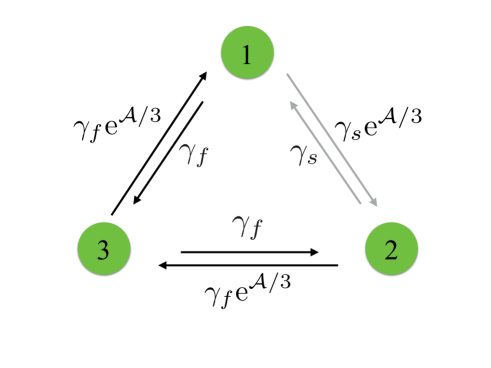
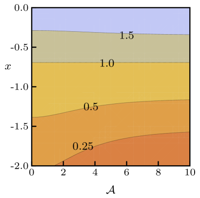
Figure 1: Brownian clock with three states. (a) Particular transition rates for the calculations. (b) Contour plot of $D_{\tau}/D_{J}$ for $\gamma_{f}=1$, where $\gamma_{s}=\textrm{e}^{x}$. The black lines represent the values $D_{\tau}/D_{J}=0.25,0.5,1.0,1.5$.

Setting $N=3$ and the transition rates to the values shown in Fig. 1, where $\gamma_{s}$ gives the time-scale for transitions between states $1$ and $2$ and $\gamma_{f}$ gives the time scale for the other transitions, we obtain the following expressions for the dispersions

$$D_{\tau}=\frac{\gamma_{s}^{2}\left(1+\mathrm{e}^{\mathcal{A}/3}\right)\left[\gamma_{f}^{2}\mathrm{e}^{\mathcal{A}/3}+\gamma_{s}\gamma_{f}\left(3-2\mathrm{e}^{\mathcal{A}/3}+3\mathrm{e}^{2\mathcal{A}/3}\right)+4\gamma_{s}^{2}\mathrm{e}^{\mathcal{A}/3}\right]}{\left(1+\mathrm{e}^{\mathcal{A}/3}+\mathrm{e}^{2\mathcal{A}/3}\right)\left(\gamma_{f}+2\gamma_{s}\right)^{3}}$$ (34)

and

$$D_{J}=\frac{\gamma_{s}\gamma_{f}(1+\mathrm{e}^{\mathcal{A}/3})\left[\gamma_{f}^{2}(1-\mathrm{e}^{\mathcal{A}/3}+\mathrm{e}^{2\mathcal{A}/3})+4\gamma_{s}\gamma_{f}\mathrm{e}^{\mathcal{A}/3}+2\gamma_{s}^{2}(1+\mathrm{e}^{2\mathcal{A}/3})\right]}{2(1+\mathrm{e}^{\mathcal{A}/3}+\mathrm{e}^{2\mathcal{A}/3})(\gamma_{f}+2\gamma_{s})^{3}},$$ (35)

where the first expression follows from Eq. (23) and the second expression can be calculated with the methods explained in [33].

In Fig. 1, we show a contour plot of the ratio $D_{\tau}/D_{J}$. If this ratio is smaller than 1 then the time random variable gives a higher precision than the current random variable. For small $\gamma_{s}$ the time random variable becomes more precise than the current random variable, with the crossover at $D_{\tau}/D_{J}=1$ displaying a weak dependence on the affinity $\mathcal{A}$.

In order to analyze the relation between dissipation and precision for this second random variable we consider the product

$$\mathcal{C}\epsilon_{\tau}^{2}=\frac{2D_{\tau}\sigma}{v_{\tau}^{2}}.$$ (36)

The average probability current in the stationary state is

$$v_{\tau}=\frac{\gamma_{s}\gamma_{f}\left(\mathrm{e}^{\mathcal{A}/3}-1\right)}{\gamma_{f}+2\gamma_{s}},$$ (37)

which gives

$$\mathcal{C}\epsilon_{\tau}^{2}=\frac{2\mathcal{A}\gamma_{s}\left(1+\mathrm{e}^{\mathcal{A}/3}\right)\left[\gamma_{f}^{2}\mathrm{e}^{\mathcal{A}/3}+\gamma_{s}\gamma_{f}\left(3-2\mathrm{e}^{\mathcal{A}/3}+3\mathrm{e}^{2\mathcal{A}/3}\right)+4\gamma_{s}^{2}\mathrm{e}^{\mathcal{A}/3}\right]}{\gamma_{f}\left(\mathrm{e}^{\mathcal{A}/3}-1\right)\left(1+\mathrm{e}^{\mathcal{A}/3}+\mathrm{e}^{2\mathcal{A}/3}\right)\left(\gamma_{f}+2\gamma_{s}\right)^{2}}.$$ (38)

For $\gamma_{s}\ll\gamma_{f}$ the product goes to zero as $\mathcal{C}\epsilon_{\tau}^{2}\sim\gamma_{s}/\gamma_{f}$. Hence, in the limit $\gamma_{s}/\gamma_{f}\to 0$ the energetic cost of an uncertainty $\epsilon$ can be arbitrarily low, in contrast to the thermodynamic uncertainty relation expressed in Eq. (31). This drastic difference constitutes the main physical insight of this paper. We have explicitly demonstrated that the fundamental tradeoff between energy and precision depends on the random variable we select.

This fundamental difference comes from the different scaling of the dispersion $D_{J}$ and $D_{\tau}$ in the limit $\gamma_{s}\ll\gamma_{f}$. The dispersion $D_{J}$ scales in the same way as the current $v_{J}$, with $D_{J}\sim\gamma_{s}$. However, the dispersion $D_{\tau}$ scales as $D_{\tau}\sim\gamma_{s}^{2}/\gamma_{f}$. This relation is easy to understand. The dispersion associated with $\tau_{m}$, for $m=1,2,3$, is proportional to the fast time-scale $\gamma_{f}^{-1}$, since the escape rates of all states are of order $\gamma_{f}$. Since the constants in Eq. (32) are the slow rates, the dispersion $D_{\tau}$ scales with the square of the constants $\gamma_{s}^{2}$ multiplied by the fast time scale $\gamma_{f}^{-1}$.

An essential difference between $\tau$ and $J$ is the following. Kirchhoff’s law is valid for $J$ even at the level of stochastic trajectories [44]. Hence, not only the average current is the same for the three links in the model but the dispersion is also independent of the link we choose to count the transitions. Both $v_{J}$ and $D_{J}$ are proportional to $\gamma_{s}$. For the random variable $\tau$, the average velocity does not depend on the link, i.e., if we take $\tau^{\prime}\equiv\tau_{2}w_{2}^{+}-\tau_{3}w_{2}^{-}$, its average is the same as the average of $\tau$ in Eq. (32). However, the dispersion related to $\tau$ is generally different from the dispersion related to $\tau^{\prime}$.

Even though our result was obtained with a simple three state model, it constitutes a general principle valid for any Markov process: there is no minimal amount of energy that must be consumed in order to achieve a certain precision quantified by a random variable of the form given in Eq. (32). We can simply follow the same strategy for arbitrary $N$ in a unicyclic network. Setting the rates associated with the link related to $\tau$ much slower than the other transition rates leads to a vanishing product $\mathcal{C}\epsilon_{\tau}^{2}$. Since a multicyclic network can always have rates in such a way that it behaves effectively like a unicyclic network [2], this result also extends to arbitrary networks.

The fact that the time random variable can lead to a limit of dissipation-less precision should not be confused with the results from [26]. In this reference, a dissipation-less clock, with its precision characterized by the current random variable, can be obtained for systems that are driven out of equilibrium by an external periodic protocol, which are different from systems driven by a fixed thermodynamic force like the one considered here.

5 Conclusion

We have obtained an expression in terms of the transition rates for the dispersion of the time a stochastic trajectory spends in a cluster of states of a unicyclic network. The unicyclic network can have an arbitrary number of states with inhomogeneous transition rates. Our expression should be an important tool for applications in which this random variable is an observable of interest, like for a cell that estimates the concentration of an external ligand.

With the help of this expression we have analyzed the tradeoff between precision and dissipation in a simple three state model. We have shown that if the precision of a Brownian clock is characterized by the time random variable from Eq. (32), we can have a precise clock that dissipates an arbitrarily small amount of energy. This result is in contrast to the thermodynamic uncertainty relation for the current, showing that the trade-off between precision and dissipation is fundamentally different for these two random variables.

While the current random variable seems like a more natural choice to quantify the precision of a Brownian clock, with a simple physical interpretation like the number of products generated in a chemical reaction, the time random variable proposed here is, in principle, also a valid choice to quantify the precision. It would be interesting to build models that also include the thermodynamic cost of an internal observer that can keep track of these random variables. Intuitively, one expects that the energetic cost of the observer that monitors the time random variable should be higher, as keeping track of $\tau$ seems to require a more sophisticated observer.

Investigating the relation between precision and dissipation in more elaborate models from biophysics constitutes a promising direction for future research [28]. One lesson to learn from our results is that when we talk about fundamental limits of precision in biological systems subjected to large fluctuations, these limits are very much dependent on the random variable we choose to characterize the precision.

Acknowledgements
We thank Édgar Roldán for carefully reading the manuscript.

Appendix A Calculation of the dispersion

In this appendix we obtain the expressions from Sec. 3 that determine the dispersion $D_{\tau}$. If we discretize time with a time step $\Delta$, the random variable $\tau_{m}$ becomes the number of time steps the trajectory is in state $m$. In this case, according to the Donsker-Varadhan theory the scaled cumulant generating function associated with $\tau$ in Eq. (5) is given by the maximum eigenvalue of a modified generator [45]. This modified generator takes the following form

$$\left[\mathcal{K}(z)\right]_{ij}=\begin{cases}\left[1-\Delta\left(w_{i}^{+}+w_{i-1}^{-}\right)\right]\mathrm{e}^{z\alpha_{i}}&\text{if}\ j=i\\ \Delta w_{i}^{+}\mathrm{e}^{z\alpha_{i}}&\text{if}\ j=i+1\\ \Delta w_{i-1}^{-}\mathrm{e}^{z\alpha_{i}}&\text{if}\ j=i-1\\ 0&\text{otherwise}.\end{cases}$$ (39)

Following Ref. [33], the first and second moments of $\tau$ can also be obtained in terms of the coefficients of the characteristic polynomial of $\mathcal{K}(z)$. Defining such coefficients as

$$|\mathcal{R}(z)|\equiv|y\mathcal{I}-\mathcal{K}(z)|\equiv\sum_{n=0}^{N}c_{n}(z)y^{n},$$ (40)

we obtain the velocity $v_{\tau}$ and dispersion $D_{\tau}$ as

$$v_{\tau}=-\frac{\sum_{n=0}^{N}c_{n}^{\prime}}{\sum_{n=1}^{N}nc_{n}}$$ (41)

and

$$D_{\tau}=-\frac{1}{2}\lim_{\Delta\rightarrow 0}\Delta\frac{\sum_{n=0}^{N}c_{n}^{\prime\prime}+2v_{\tau}\sum_{n=1}^{N}nc_{n}^{\prime}+v_{\tau}^{2}\sum_{n=2}^{N}n(n-1)c_{n}}{\sum_{n=1}^{N}nc_{n}}.$$ (42)

The lack of explicit $z$-dependence of the coefficients denotes evaluation at $z=0$ and the primes denote derivatives with respect to $z$. Since we are interested in the results in continuous time, the limit $\Delta\to 0$ is taken in the above equation.
Each coefficient $c_{n}(z)$ in Eq. (40) is an $(N-n)$th order polynomial in $\Delta$, i.e.,

$$c_{n}(z)\equiv\sum_{k=0}^{N-n}\tilde{c_{n}}^{(k)}(z)\;\Delta^{k}.$$ (43)

Combining Eqs. (41) and (43), we get

$$v_{\tau}=-\frac{\sum_{k=0}^{N}\left(\sum_{n=0}^{N-k}\tilde{c_{n}}^{\prime(k)}\right)\Delta^{k}}{\sum_{k=0}^{N}\left(\sum_{n=1}^{N-k}n\tilde{c_{n}}^{(k)}\right)\Delta^{k}}.$$ (44)

The above equation express $v_{\tau}$ as a ratio of two polynomials in $\Delta$. We find that for all $k\neq N-1$, the coefficients of these two polynomials vanish and only the contribution of order $\mathcal{O}(\Delta^{N-1})$ survives, which leads to Eq. (22). Combining Eqs. (42) and (43), we obtain

$$D_{\tau}=-\lim_{\Delta\to 0}\Delta\left[\frac{\sum_{k=0}^{N}\left(\sum_{n=0}^{N-k}\tilde{c_{n}}^{\prime\prime(k)}+2v_{\tau}\sum_{n=1}^{N-k}n\tilde{c_{n}}^{\prime(k)}+v_{\tau}^{2}\sum_{n=2}^{N-k}n(n-1)\tilde{c_{n}}^{(k)}\right)\Delta^{k}}{2\sum_{k=0}^{N}\left(\sum_{n=1}^{N-k}n\tilde{c_{n}}^{(k)}\right)\Delta^{k}}\right],$$ (45)

where $v_{\tau}$ is given by Eq. (22). In this case, only the terms of order $\mathcal{O}(\Delta^{N-2})$ or higher do not vanish in the numerator, while in the denominator the sole contribution comes from the terms of order $\mathcal{O}(\Delta^{N-1})$, which leads to Eq. (23).

An expression for the coefficients $\tilde{c_{n}}^{(k)}(z)$ as functions of the transition rates can be obtained in the following way. From Eqs. (39) and (40), we get

$$\mathcal{R}(z)\leavevmode\resizebox{433.62pt}{}{$\equiv\left(\begin{array}[]{@{}*8c}y-\mathrm{e}^{z\alpha_{1}}[1-\Delta\lambda_{1}]&-\mathrm{e}^{z\alpha_{1}}\Delta w_{1}^{-}&0&\cdots&\cdots&\cdots&0&-\mathrm{e}^{z\alpha_{1}}\Delta w_{N}^{+}\\ -\mathrm{e}^{z\alpha_{2}}\Delta w_{1}^{+}&y-\mathrm{e}^{z\alpha_{2}}[1-\Delta\lambda_{2}]&-\mathrm{e}^{z\alpha_{2}}\Delta w_{2}^{-}&0&\cdots&\cdots&\cdots&0\\ 0&-\mathrm{e}^{z\alpha_{3}}\Delta w_{2}^{+}&y-\mathrm{e}^{z\alpha_{3}}[1-\Delta\lambda_{3}]&-\mathrm{e}^{z\alpha_{3}}\Delta w_{3}^{-}&0&\cdots&\cdots&0\\ \vdots&\vdots&\vdots&\vdots&\vdots&\vdots&\vdots&\vdots\\ -\mathrm{e}^{z\alpha_{N}}\Delta w_{N}^{-}&0&\cdots&\cdots&\cdots&0&-\mathrm{e}^{z\alpha_{N}}\Delta w_{N-1}^{+}&y-\mathrm{e}^{z\alpha_{N}}[1-\Delta\lambda_{N}]\\ \end{array}\right),$}$$ (51)

where $\lambda_{m}\equiv(w_{m}^{+}+w_{m-1}^{-})$ is the escape rate from state $m$, as defined in Eq. (8). The determinant of the $(1\times 1)$ submatrix of $\mathcal{R}(z)$ starting from its upper left corner is written as

$$d_{1}(z)\equiv[\mathcal{R}(z)]_{11}=y-\mathrm{e}^{z\alpha_{1}}[1-\Delta\lambda_{1}].$$ (52)

The determinant $d_{2}(z)$ of the $(2\times 2)$ submatrix of $\mathcal{R}(z)$ starting from its upper left corner can be expressed in terms of $d_{1}(z)$ as

$$d_{2}(z)=\left[y-\mathrm{e}^{z\alpha_{2}}(1-\Delta\lambda_{2})\right]d_{1}(z)-\mathrm{e}^{z(\alpha_{1}+\alpha_{2})}\Delta^{2}\nu_{1}.$$ (53)

In a similar way, $d_{j}(z)$, the determinant for the $(j\times j)$ submatrix of $\mathcal{R}(z)$ starting from its upper left corner for $3\leq j\leq N$ can be expressed by the general recursion relation [46]

$$d_{j}(z)=\left[y-\mathrm{e}^{z\alpha_{j}}(1-\Delta\lambda_{j})\right]d_{j-1}(z)-\mathrm{e}^{z(\alpha_{j-1}+\alpha_{j})}\Delta^{2}\nu_{j-1}d_{j-2}(z),$$ (54)

where $\nu_{m}\equiv w_{m}^{+}w_{m}^{-}$, as defined in Eq. (9). This relation is valid only for a tridiagonal matrix and, hence, $d_{N}(z)\neq|\mathcal{R}(z)|$.

To account for the terms in $|\mathcal{R}(z)|$ that appear due to the presence of the non-zero elements $[\mathcal{R}(z)]_{1N}$ and $[\mathcal{R}(z)]_{N1}$, we define a second kind of determinant, starting from one element left and one below from the upper left corner of $\mathcal{R}(z)$. Such determinant for the $(1\times 1)$ submatrix of $\mathcal{R}(z)$ is

$$d_{1}^{\star}(z)\equiv[\mathcal{R}(z)]_{22}=y-\mathrm{e}^{z\alpha_{2}}[1-\Delta\lambda_{2}].$$ (55)

The determinant $d_{2}^{\star}(z)$ of the $(2\times 2)$ submatrix can be expressed in terms of $d_{1}^{\star}(z)$ as

$$d_{2}^{\star}(z)=\left[y-\mathrm{e}^{z\alpha_{3}}(1-\Delta\lambda_{3})\right]d_{1}^{\star}(z)-\mathrm{e}^{z(\alpha_{2}+\alpha_{3})}\Delta^{2}\nu_{2}.$$ (56)

In a similar manner, $d_{j}^{\star}(z)$, the determinant for the $(j\times j)$ submatrix of $\mathcal{R}(z)$ starting from $[\mathcal{R}(z)]_{22}$ for $3\leq j\leq N-1$ is given by the recursion relation

$$d_{j}^{\star}(z)=[y-\mathrm{e}^{z\alpha_{j+1}}(1-\Delta\lambda_{j+1})]d_{j-1}^{\star}(z)-\mathrm{e}^{z(\alpha_{j}+\alpha_{j+1})}\Delta^{2}\nu_{j}d_{j-2}^{\star}(z)$$ (57)

We can now express $|\mathcal{R}(z)|$ in terms of these two types of determinants as [46]

$$|\mathcal{R}(z)|=d_{N}(z)-d_{N-2}^{\star}(z)\;\Delta^{2}\nu_{N}\mathrm{e}^{z(\alpha_{1}+\alpha_{N})}-\Delta^{N}(w_{1}^{+}w_{2}^{+}...w_{N}^{+}+w_{1}^{-}w_{2}^{-}...w_{N}^{-})\mathrm{e}^{z\theta_{N}},$$ (58)

where $\theta_{N}=\alpha_{1}+\alpha_{2}+...+\alpha_{N}$.

From Eq. (51), we get that $d_{j}(z)$ and $d_{j}^{\star}(z)$ are $j-th$ order polynomials in $y$. Thus we define

$$d_{j}(z)=\sum_{n=0}^{j}a_{j}^{(n)}(z)y^{n}$$ (59)

and

$$d_{j}^{\star}(z)=\sum_{n=0}^{j}a_{j}^{\star(n)}(z)y^{n}.$$ (60)

From Eqs. (40), (58), (59) and (60), we obtain

$$c_{n}(z)=a_{N}^{(n)}(z)-\nu_{N}\Delta^{2}a_{N-2}^{\star(n)}(z)\mathrm{e}^{z(\alpha_{1}+\alpha_{N})}-\delta_{n,0}\left[\Delta^{N}(w_{1}^{+}w_{2}^{+}...w_{N}^{+}+w_{1}^{-}w_{2}^{-}...w_{N}^{-})\mathrm{e}^{z\theta_{N}}\right].$$ (61)

Combining Eqs. (54) and (59), we get the recursion relation

$$a_{j}^{(n)}(z)=a_{j-1}^{(n-1)}(z)-a_{j-1}^{(n)}(z)\;\mathrm{e}^{z\alpha_{j}}\left[1-\Delta\lambda_{j}\right]-a_{j-2}^{(n)}(z)\;\Delta^{2}\nu_{j-1}\mathrm{e}^{z(\alpha_{j-1}+\alpha_{j})},$$ (62)

where $a_{j}^{(n)}(z)\neq 0$ for $0\leq j\leq N$ and $0\leq n\leq j$. Utilizing Eq. (59) for $j=1$, we get the initial values for the recursion relation as $a_{1}^{(0)}(z)=-\mathrm{e}^{z\alpha_{1}}[1-\Delta\lambda_{1}]$ and $a_{1}^{(1)}(z)=1$. In addition, we define $a_{0}^{(0)}(z)=1$. From Eqs. (57) and (60), we establish a similar kind of recursion relation for $a_{j}^{\star(n)}(z)$

$$a_{j}^{\star(n)}(z)=a_{j-1}^{\star(n-1)}(z)-a_{j-1}^{\star(n)}(z)\;\mathrm{e}^{z\alpha_{j+1}}\left[1-\Delta\lambda_{j+1}\right]-a_{j-2}^{\star(n)}(z)\;\Delta^{2}\nu_{j}\mathrm{e}^{z(\alpha_{j}+\alpha_{j+1})},$$ (63)

where $a_{j}^{\star(n)}(z)\neq 0$ for $0\leq j\leq N-2$ and $0\leq n\leq j$. From Eq. (60) for $j=1$, the initial values for the above recursion are obtained as $a_{1}^{\star(0)}(z)=-\mathrm{e}^{z\alpha_{2}}[1-\Delta\lambda_{2}]$, $a_{1}^{\star(1)}(z)=1$ and we define $a_{0}^{\star(0)}(z)=1$.

Since each coefficient $a_{j}^{(n)}(z)$ [or $a_{j}^{\star(n)}(z)$] is a $(j-n)$th order polynomial in $\Delta$, we define

$$a_{j}^{(n)}(z)=\sum_{k=0}^{j-n}b_{jn}^{(k)}(z)\;\Delta^{k}$$ (64)

and

$$a_{j}^{\star(n)}(z)=\sum_{k=0}^{j-n}b_{jn}^{\star(k)}(z)\;\Delta^{k}.$$ (65)

From Eqs. (43), (61), (64) and (65), we obtain

$$\tilde{c_{n}}^{(k)}(z)=b_{Nn}^{(k)}(z)-\nu_{N}b_{(N-2)n}^{\star(k-2)}(z)\;\mathrm{e}^{z(\alpha_{1}+\alpha_{N})}-\delta_{n,0}\delta_{k,N}\left[(w_{1}^{+}w_{2}^{+}...w_{N}^{+}+w_{1}^{-}w_{2}^{-}...w_{N}^{-})\mathrm{e}^{z\theta_{N}}\right],$$ (66)

where $\delta_{n,0}$ and $\delta_{k,N}$ are Kronecker deltas. Eqs. (62) and (64) lead to the following recursion relation

$$b_{jn}^{(k)}(z)=b_{(j-1)(n-1)}^{(k)}(z)-\left[b_{(j-1)n}^{(k)}(z)-\lambda_{j}b_{(j-1)n}^{(k-1)}(z)\right]\mathrm{e}^{z\alpha_{j}}-b_{(j-2)n}^{(k-2)}(z)\;\nu_{j-1}\mathrm{e}^{z(\alpha_{j-1}+\alpha_{j})},$$ (67)

where $b_{jn}^{(k)}(z)\neq 0$ for $0\leq j\leq N$, $0\leq n\leq j$ and $0\leq k\leq j-n$. For $j=0$, the only possible values of $(j,n,k)$ are $(0,0,0)$ and for $j=1$, there are $(1,0,0)$, $(1,0,1)$ and $(1,1,0)$. Thus the initial values for the above recursion are given by the four coefficients $b_{00}^{(0)}(z)=1$, $b_{10}^{(0)}(z)=-\mathrm{e}^{z\alpha_{1}}$, $b_{10}^{(1)}(z)=\lambda_{1}\mathrm{e}^{z\alpha_{1}}$ and $b_{11}^{(0)}(z)=1$. In a similar manner, the coefficients $b_{jn}^{\star(k)}(z)$ are given by the recursion relation

$$b_{jn}^{\star(k)}(z)=b_{(j-1)(n-1)}^{\star(k)}(z)-\left[b_{(j-1)n}^{\star(k)}(z)-\lambda_{j+1}b_{(j-1)n}^{\star(k-1)}(z)\right]\mathrm{e}^{z\alpha_{j+1}}-b_{(j-2)n}^{\star(k-2)}(z)\;\nu_{j}\mathrm{e}^{z(\alpha_{j}+\alpha_{j+1})},$$ (68)

where $b_{jn}^{\star(k)}(z)\neq 0$ for $0\leq j\leq N-2$, $0\leq n\leq j$ and $0\leq k\leq j-n$. The initial values in this case are $b_{00}^{\star(0)}(z)=1$, $b_{10}^{\star(0)}(z)=-\mathrm{e}^{z\alpha_{2}}$, $b_{10}^{*(1)}(z)=\lambda_{2}\mathrm{e}^{z\alpha_{2}}$ and $b_{11}^{\star(0)}(z)=1$.

The solution of Eq. (67) is

$$b_{jn}^{(k)}(z)=(-1)^{j-n-k}g_{j}(z)\sum_{k_{2}=0}^{\lfloor\frac{k}{2}\rfloor}(-1)^{k_{2}}S_{j,n,k,k_{2}}(z),$$ (69)

where $g_{j}(z)\equiv\mathrm{e}^{z(\alpha_{1}+\alpha_{2}+...+\alpha_{j})}$. The terms $S_{j,n,k,k_{2}}(z)$ in the above expression are given by

$$S_{j,n,k,k_{2}}(z)\equiv T^{(\nu)}_{j,k_{2}}\times T^{(\lambda)}_{j,k,k_{2}}\times T^{(\mu)}_{j,n,k,k_{2}}(z),$$ (70)

where

$$T^{(\nu)}_{j,k_{2}}\equiv\sum_{l_{1}=1}^{j-2k_{2}+1}\;\;\sum_{l_{2}=l_{1}+2}^{j-2k_{2}+3}\;\;\sum_{l_{3}=l_{2}+2}^{j-2k_{2}+5}...\sum_{l_{k_{2}}=l_{k_{2}-1}+2}^{j-1}\nu_{l_{1}}\nu_{l_{2}}\nu_{l_{3}}...\nu_{l_{k_{2}}},$$ (71)

$$T^{(\lambda)}_{j,k,k_{2}}\equiv\sum_{p_{\lambda}=1}^{\textbf{C}(j-2k_{2},k_{1})}\;\;\prod_{q_{\lambda}=1}^{k_{1}}\lambda_{[\textbf{M}_{\bar{\Omega}(j,\textbf{L}),k_{1}}]_{p_{\lambda},q_{\lambda}}},$$ (72)

and

$$T^{(\mu)}_{j,n,k,k_{2}}(z)\equiv\sum_{p_{\mu}=1}^{\textbf{C}(j-k,n)}\;\;\prod_{q_{\mu}=1}^{n}\mu_{[\textbf{M}_{\bar{\Omega}_{2}(j,\textbf{L},p_{\lambda}),n}]_{p_{\mu},q_{\mu}}}.$$ (73)

Here $\mu_{j}(z)\equiv\textrm{e}^{-z\alpha_{j}}$ and the matrix M is introduced in Sec. 3. The solution of Eq. (68) is

$$b_{jn}^{\star(k)}(z)=(-1)^{j-n-k}g^{\star}_{j}(z)\sum_{k_{2}=0}^{\lfloor\frac{k}{2}\rfloor}(-1)^{k_{2}}S^{\star}_{j,n,k,k_{2}}(z),$$ (74)

where $g^{\star}_{j}(z)\equiv\mathrm{e}^{z(\alpha_{2}+\alpha_{3}+...+\alpha_{j+1})}$,

$$S^{\star}_{j,n,k,k_{2}}(z)\equiv T^{\star(\nu)}_{j,k_{2}}\times T^{\star(\lambda)}_{j,k,k_{2}}\times T^{\star(\mu)}_{j,n,k,k_{2}},$$ (75)

$$T^{\star(\nu)}_{j,k_{2}}\equiv\sum_{l^{\star}_{1}=2}^{j-2k_{2}+2}\;\;\sum_{l^{\star}_{2}=l^{\star}_{1}+2}^{j-2k_{2}+4}\;\;\sum_{l^{\star}_{3}=l^{\star}_{2}+2}^{j-2k_{2}+6}\cdots\sum_{l^{\star}_{k_{2}}=l^{\star}_{k_{2}-1}+2}^{j}\nu_{l^{\star}_{1}}\nu_{l^{\star}_{2}}\nu_{l^{\star}_{3}}...\nu_{l^{\star}_{k_{2}}},$$ (76)

$$T^{\star(\lambda)}_{j,k,k_{2}}\equiv\sum_{p_{\lambda}=1}^{\textbf{C}(j-2k_{2},k_{1})}\;\;\prod_{q_{\lambda}=1}^{k_{1}}\lambda_{[\textbf{M}_{\bar{\Omega}^{\star}(j,\textbf{L}),k_{1}}]_{p_{\lambda},q_{\lambda}}},$$ (77)

and

$$T^{\star(\mu)}_{j,n,k,k_{2}}\equiv\sum_{p_{\mu}=1}^{\textbf{C}(j-k,n)}\;\;\prod_{q_{\mu}=1}^{n}\mu_{[\textbf{M}_{\bar{\Omega}^{\star}_{2}(j,\textbf{L},p_{\lambda}),n}]_{p_{\mu},q_{\mu}}}.$$ (78)

Eq. (66) along with Eqs. (69 $-$ 78) leads to an expression of the coefficients $\tilde{c}^{(k)}_{n}(z)$ in terms of the transition rates. Taking derivatives of this coefficients and setting $z=0$ we obtain the expressions from Sec. 3.

References

References

- [1] Barato A C and Seifert U 2015 Phys. Rev. Lett. 114 158101
- [2] Barato A C and Seifert U 2015 J. Phys. Chem. B 119 6555
- [3] Pietzonka P, Barato A C and Seifert U 2016 Phys. Rev. E 93 052145
- [4] Pietzonka P, Barato A C and Seifert U 2016 J. Phys. A: Math. Theor. 49 34LT01
- [5] Gingrich T R, Horowitz J M, Perunov N and England J L 2016 Phys. Rev. Lett. 116 120601
- [6] Polettini M, Lazarescu A and Esposito M 2016 Phys. Rev. E 94 052104
- [7] Gingrich T R, Rotskoff G M and Horowitz J M 2017 J. Phys. A: Math. Theor. 50 184004
- [8] Rotskoff G M 2017 Phys. Rev. E 95, 030101
- [9] Saito K and Dhar A 2016 EPL 114 50004
- [10] Neri I, Roldan E, Dörpinghaus M, Meyr H and Jülicher F 2015 Phys. Rev. Lett. 115 250602
- [11] Neri I, Roldan E and Jülicher F 2017 Phys. Rev. X 7, 011019
- [12] Garrahan J P 2017 Phys. Rev. E 95, 032134
- [13] Qian H 2007 Annu. Rev. Phys. Chem. 58 113
- [14] Lan G, Sartori P, Neumann S, Sourjik V and Tu Y 2012 Nature Phys. 8 422
- [15] Mehta P and Schwab D J 2012 Proc. Natl. Acad. Sci. U.S.A. 109 17978
- [16] Barato A C, Hartich D and Seifert U 2013 Phys. Rev. E 87 042104
- [17] De Palo G and Endres R G 2013 PLoS Comput. Biol. 9 e1003300
- [18] Govern C C and ten Wolde P R 2014 Proc. Natl. Acad. Sci. U.S.A. 111 17486
- [19] Govern C C and ten Wolde P R 2014 Phys. Rev. Lett. 113 258102
- [20] Hartich D, Barato A C and Seifert U 2015 New J. Phys. 17 055026
- [21] Sartori P, Granger L, Lee C F and Horowitz J M 2014 PLoS Comput. Biol. 10 e1003974
- [22] Barato A C, Hartich D and Seifert U 2014 New J. Phys. 16 103024
- [23] Bo S, Del Giudice M and Celani A 2015 J. Stat. Mech.: Theor. Exp. 2015 P01014
- [24] Ito S and Sagawa T 2015 Nat. Commun. 6 7498
- [25] McGrath T, Jones N S, ten Wolde P R and Ouldridge T E 2017 Phys. Rev. Lett. 118 028101
- [26] Barato A C and Seifert U 2016 Phys. Rev. X 6 041053
- [27] Ferrell J E, Tsai T Y C and Yang Q 2011 Cell 144 874
- [28] Cao Y, Wang H, Ouyang Q and Tu Y 2015 Nature Phys. 11 772
- [29] Dong G and Golden S S 2008 Curr. Opin. Microbiol. 11 541
- [30] Seifert U 2012 Rep. Prog. Phys. 75 126001
- [31] Derrida B 1983 J. Stat. Phys. 31 433
- [32] Koza Z 1999 J. Phys. A: Math. Gen. 32 7637
- [33] Barato A C and Seifert U 2015 Phys. Rev. E 92 032127
- [34] Berg H C and Purcell E M 1977 Biophys. J. 20 193
- [35] Bialek W and Setayeshgar S 2005 Proc. Natl. Acad. Sci. U.S.A. 102 10040
- [36] Endres R G and Wingreen N S 2008 Proc. Natl. Acad. Sci. U.S.A. 105 15749
- [37] Endres R G and Wingreen N S 2009 Phys. Rev. Lett. 103 158101
- [38] Mora T and Wingreen N S 2010 Phys. Rev. Lett. 104 248101
- [39] Govern C C and ten Wolde P R 2012 Phys. Rev. Lett. 109 218103
- [40] Kaizu K, de Ronde W, Paijmans J, Takahashi K, Tostevin F and ten Wolde P R 2014 Biophys. J. 106 976
- [41] Li G and Qian H 2002 Traffic 3 249
- [42] Lang A H, Fisher C K, Mora T and Mehta P 2014 Phys. Rev. Lett. 113 148103
- [43] Barato A C and Chetrite R 2015 J. Stat. Phys. 160 1154
- [44] Barato A C and Chetrite R 2012 J. Phys. A: Math. Theor. 45 485002
- [45] Touchette H 2009 Phys. Rep. 478 1-69
- [46] Chemla Y R, Moffitt J R and Bustamante C 2008 J. Phys. Chem. B 112 6025