Constraining $Z^{\prime}$ widths from $p_{T}$ measurements in Drell-Yan processes

Abstract

Abstract

We define a Focus Point (FP) Asymmetry, $A_{\rm FP}$, obtained by integrating the normalised transverse momentum distribution of either lepton produced in the Drell-Yan (DY) process below and above a point where a variety of popular $Z^{\prime}$ models all have the same magnitude. For a given $Z^{\prime}$ mass the position of this FP is predictable, depending only on the collider energy and on the low transverse momentum cut chosen in the normalisation procedure. The resulting $A_{\rm FP}$ is very sensitive to the $Z^{\prime}$ width and can be used to constrain this parameter in experimental fits.

I Introduction

Additional massive neutral gauge bosons, also known as $Z^{\prime}$s, are ubiquitous in Beyond Standard Model (BSM) scenarios. Experimentally such states can be observed in invariant mass spectra formed using the decay products of the $Z^{\prime}$ in for example a di-lepton mass spectrum. The new physics signal has some peaking structure, concentrated in some interval centred around its mass. Experimental searches for such heavy states often assume that such a resonance can be described by a Breit-Wigner (BW) line-shape, above a smooth SM background.

A $Z^{\prime}$ resonance can have a wide range of intrinsic widths, which depend on the scenario considered. It can be narrow, as for example, in $E_{6}$, Generalised Left-Right (GLR) symmetric and Generalised Standard Model (GSM) scenarios Accomando et al. (2011), where $\Gamma_{Z^{\prime}}/M_{Z^{\prime}}\sim 0.5-10\%$. Alternatively, it can be wide, as in Technicolour Belyaev et al. (2009) scenarios, Composite Higgs Models Barducci et al. (2013) or in more generic models where the $Z^{\prime}$ boson coupling to the first two fermion generations is different to that the the third generation Kim and Lee (2014); Malkawi and Yuan (2000). The $Z^{\prime}$ can also interact with the SM gauge bosons in presence of $Z/Z^{\prime}$ mixing Altarelli et al. (1989). In all of these cases large $\Gamma_{Z^{\prime}}/M_{Z^{\prime}}$ values, up to $\sim 50\%$, are induced by the additional $Z^{\prime}$ decay channels available in all such cases. When very wide the resonance does not have a well-defined BW line-shape and appears as a broad shoulder over the SM background.

The most generic experimental analyses look for narrow resonances where the experimental resolution is the dominant contribution to the observable width of a peak structure appearing over a SM background. In this approach, theoretical cross section predictions for specific models are usually calculated in the Narrow Width Approximation (NWA). Finite Width (FW) and interference effects can be taken into account in a model independent way following the approach described in Accomando et al. (2013). Up to date experimental bounds on narrow (i.e., where $\Gamma_{Z^{\prime}}/M_{Z^{\prime}}\sim 1\%$) $Z^{\prime}$ resonances have been released from CMS Collaboration (2016) and ATLAS collaboration (2017) with the Run 2 energy of 13 TeV and an integrated luminosity of 13 fb^-1 and 36.1 fb^-1 respectively. The most stringent bounds set the limit for the masses of these objects $M_{Z^{\prime}}>4$ TeV. For wider $Z^{\prime}$s, the experimental collaborations look for both resonances and effectively very wide resonances in non-resonant searches. In the first case, ATLAS has provided us with acceptance curves that can be used to rescale the limits obtained for narrow resonances, for widths up to 5–10% of the mass at the most collaboration (2017). In the second (‘effectively’ non-resonant case, where the width-to-mass region can be over 10%), the experimental analyses are essentially counting experiments: an excess of events is searched for above an estimated SM background. These last searches optimize selection criteria in the context of particular specific models order to maximise the discovery/exclusion potential at the LHC. The experimental results heavily rely on the good understanding and control of the SM background. In this case, the use of charge asymmetries may be useful in extracting a $Z^{\prime}$ signal Accomando et al. (2016a). (Needless to say, in the remainder, we will define benchmarks which escapes experimental limits, for any value of $\Gamma_{Z^{\prime}}/M_{Z^{\prime}}$ presented.)

If a $Z^{\prime}$ state were to be observed at the LHC determining the intrinsic width would be an immediate objective. The width would provide information about the underlying $Z^{\prime}$ model and the coupling strength and quantum numbers of the $Z^{\prime}$ in its interactions with SM objects. The measurement of a width using the mass spectrum is limited by the detector resolution in the case of a narrow resonance and for a very wide resonance (that cannot be approximated by a BW) a model specific approach would be required.

The purpose of this paper is to describe the role of an alternative observable to the di-lepton invariant mass ($M_{ll}$) that could be used to extract information on the intrinsic width of the $Z^{\prime}$. The advantage of this approach is twofold. Firstly, one can use this new observable to determine the intrinsic width of the resonance. Secondly, the latter can potentially be used to perform a constrained fit to the cross section (or charge asymmetry) in the di-lepton invariant mass, so as to disentangle the pure signal contributions from dynamics resulting from FW and/or interference effects. (While we will address the first point in this publication, we will defer treatment of the second to a forthcoming one.) This new observable is the transverse momentum distribution of an individual lepton in the final state. We will show that the corresponding (normalised) spectrum exhibits a Focus Point (FP) that is the same for all $Z^{\prime}$ models considered, the latter thereby acting similarly to the $Z^{\prime}$ pole in the di-lepton invariant mass. One can also define asymmetries around this FP, $A_{\rm FP}$s, that provide information on the underlying $Z^{\prime}$ scenario, in terms of its quantum numbers.

This is in principle analogous to the case of charge asymmetries, in practice though the FP ones display sensitivity to a different parameter. In fact, herein, we assume that a $Z^{\prime}$ state has already been observed and a (tentative) value of its mass has been extracted: this is a precondition to the exploitation of the FP and its asymmetries. With this mind, such FP observables provide one with an additional powerful diagnostic tool in understanding the nature of the $Z^{\prime}$, quite uncorrelated to the aforementioned cross section and charge asymmetries, as they display a strong sensitivity to its width, whichever the actual value of it. This is extremely important as, on the one hand, $\Gamma_{Z^{\prime}}$ contains information about all couplings of the $Z^{\prime}$ state (hence about the underlying model) and, on the other hand, neither fits to the cross section (wherein the dependence upon $\Gamma_{Z^{\prime}}$ really ought to be minimized in the search for the BW peak) nor mappings of charge asymmetries (which are primarily sensitive to the relative sign of the above couplings) offer the same scope.

This note is organized as follows. In Sect. II we introduce the new variable and describe how it can be used for the aforementioned purposes. In Sect. III we illustrate our results. Finally, we conclude in Sect. IV.

II $Z^{\prime}$s $p_{T}$ distribution spectra

In order to perform our analysis we have used the numerical code documented in Refs. Accomando et al. (2013, 2016a). Standard acceptance cuts on the leptons have been required: $p_{T}>20$ GeV and $|\eta|<2.5$. The acceptance $p_{T}$ cut is not really important in our analysis since we are going to introduce a substantial $p_{T}^{\rm min}$ cut on the leptons ($>~{}900$ GeV) when analysing our transverse momentum distribution. Moreover we have verified that tightening the pseudorapidity does not change our conclusions, as discussed in Sect. II.6. In order to speed up the numerical simulation (we will be working with very high invariant masses, of ${\cal O}(1~{}{\rm TeV})$, we require that $M_{ll}>50$ GeV.

Differential distributions for three $Z^{\prime}$ benchmark models ($E_{6}^{I}$, GLR-LR, GSM-SSM Accomando et al. (2016a)) have been generated for different $Z^{\prime}$ boson masses and widths. In computing the binned number of events, we include all the contributions to the same final state: $Z^{\prime}$ signal, SM background and their mutual interference. Higher orders corrections have not been considered in this work. Both NNLO QCD and NLO EW corrections can be large, but they also contribute with opposite signs, leading to some cancellations Balossini et al. (2008). However we are interested in the very high $p_{T}$ region, where we can assume the NNLO QCD contribution to appear as a (roughly) constant k-factor Li and Petriello (2012). The asymmetry observable that we will define in the following will naturally provide a cancellation of this effect. NLO EW corrections instead are expected to grow in magnitude with the energy, and they might lead to observable effects. Yet, no public code is available at the moment for the NLO calculation of EW radiative corrections to the leptons’ $p_{T}$ spectra in DY production including real and virtual EW gauge boson emission, both of which are needed for an accurate estimate of the effects we are studying, owing to the fact that the di-lepton final state is treated inclusively in experimental analyses (i.e., no veto is enforced against real radiation of EW gauge bosons). Hence, for the time being, we will neglect these effects too.

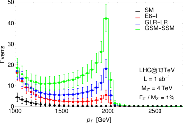
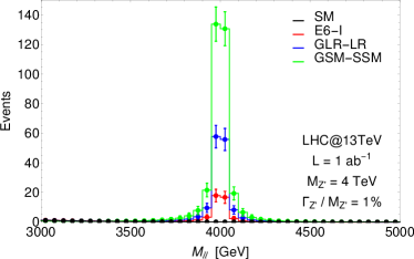
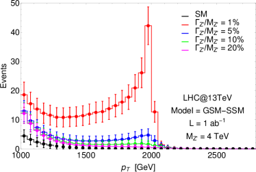
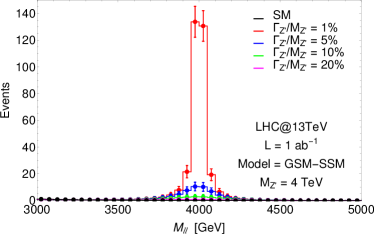
In Fig. 1 we show the $p_{T}$ and the invariant mass distributions. The data shown have been binned by integrating in the $p_{T}$ ($M_{ll}$) variable and multiplying by the quoted luminosity in order to obtain the number of events on the $y$ axis. The error bars represent the statistical error on the number of events observed in each bin and are given by the square root of the number of events in each bin. As expected in the $p_{T}$ distribution, a noticeable peak appears at $p_{T}\approx M_{Z^{\prime}}/2$ for all BSM scenarios considered with the slope leading to it varying depending on the underlying $Z^{\prime}$ model. The total number of events is defined by the model cross section. The SM distribution by contrast monotonically decreases. There is no point in $p_{T}$ amongst the various curves where all the differential cross sections have the same magnitude.

(a) (b)

Figure 1: Distribution of number of events as function of (a) the $p_{T}$ of either lepton and (b) of the di-lepton invariant mass as predicted in the SM and in three $Z^{\prime}$ benchmark models with $M_{Z^{\prime}}=4~{}{\rm TeV}$ at the 13 TeV LHC with $\mathcal{L}=1~{}ab^{-1}$. For all models the width of the resonance has been fixed at 1% of its mass. Acceptance cuts are applied ($|\eta|<2.5$), detector efficiencies are not accounted for.

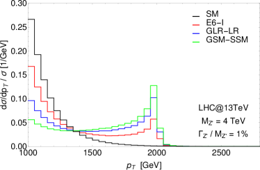
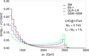
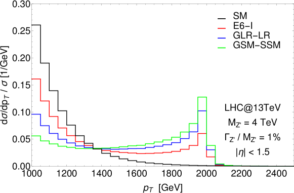
An interesting feature appears when the distributions are normalised. Starting from the differential distributions shown in Fig. 1(a) for each model in the legend, we divide the number of events in each bin by the total number of events that is obtained integrating the cross section from the chosen $p_{T}^{\rm min}$ on. For this specific case we chose $p_{T}^{\rm min}=1000$ GeV. The results of this normalisation are shown in Fig. 2(a). The most interesting feature in this plot is that around $p_{T}$ = 1400 GeV all the curves have the same magnitude. We call this intersection point the Focus Point (FP). The FP position strongly depends on the lepton $p_{T}^{\rm min}$ cut that we choose to maximise the sensitivity to the hypothetical $Z^{\prime}$ boson. This will be discussed more extensively in Sect. III.2, here we give just an example of this effect. For a $Z^{\prime}$ mass of 5 TeV the optimal choice is $p_{T}^{\rm min}=1200$ GeV. In this case we obtain very similar behaviour, albeit with the FP shifted to around 1.2 TeV, as plotted in Fig. 2(b). In these illustrations we have taken the LHC energy to be 13 TeV and use the CT14NNLO PDF set Dulat et al. (2016) evaluated at the $Q=\sqrt{\hat{s}}$ factorisation/renormalisation scale (i.e., the centre-of-mass energy at the parton level).

(a) (b)

Figure 2: Normalised distribution in $p_{T}$ of either lepton as predicted in the SM and in three $Z^{\prime}$ benchmark models at the 13 TeV LHC. For all models the width of the resonance has been fixed at 1% of its mass. Acceptance cuts are applied ($|\eta|<2.5$), detector efficiencies are not accounted for. (a) $p_{T}^{\rm min}=1000~{}{\rm GeV}$ and $M_{Z^{\prime}}=4~{}{\rm TeV}$, (b) $p_{T}^{\rm min}=1200~{}{\rm GeV}$ and $M_{Z^{\prime}}=5~{}{\rm TeV}$.

(a) (b)

Figure 3: (a) Number of events as function of $p_{T}$ of either lepton as predicted in the SM and in three $Z^{\prime}$ benchmark models with $M_{Z^{\prime}}=4~{}{\rm TeV}$ at the 13 TeV LHC with $\mathcal{L}=1~{}ab^{-1}$. The width of the resonances has been fixed at their natural value as predicted by the model. Acceptance cuts are applied ($|\eta|<2.5$), no detector efficiencies are accounted for. (b) Normalized distribution of (a) with $p_{T}^{\rm min}=1000~{}GeV$.

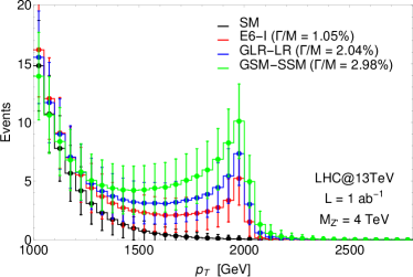
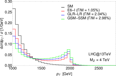
For completeness in Fig. 3 we show distributions for the number of events and the normalized $p_{T}$ for the three benchmark models with the resonance widths fixed to the natural values predicted by each model. The values for the resonance widths can be significantly modified by the presence of new physics, therefore in order to be as general as possible we will consider the $Z^{\prime}$ width to be a free parameter.

In order to understand this feature in detail, in the following section we explore its dependence upon the collider energy, the $Z^{\prime}$ parameters (its mass and width), the minimum $p_{T}$ cut and the normalisation procedure as well as the role of the interference between the $Z^{\prime}$ diagram and SM topologies. By contrast, we limit ourselves to simply state here that we have verified the independence of the FP location upon the choice of PDFs and $Q$: this should not be surprising as the quark and antiquark behaviour inside the proton at the relevant $x$ and $Q$ values is well known Accomando et al. (2016b).

II.1 The role of the partonic (or collider) energy

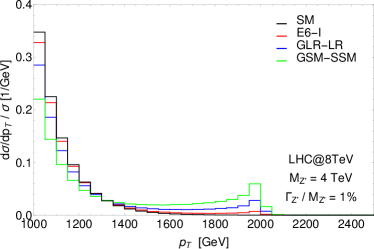
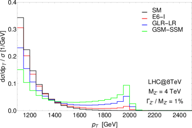
The observation is found to be is sensitive to the partonic (or collider) energy. Fig. 4 (where we have again assumed $\Gamma_{Z^{\prime}}/M_{Z^{\prime}}=1\%$) illustrates that the FP also appears at 8 TeV for different models and $Z^{\prime}$ masses considered.

(a) (b)

Figure 4: Normalised distribution in $p_{T}$ of either lepton as predicted in the SM and in three $Z^{\prime}$ benchmark models with $M_{Z^{\prime}}=4~{}{\rm TeV}$ at the 8 TeV LHC. For all models the width of the resonance has been fixed at 1% of its mass. Acceptance cuts are applied ($|\eta|<2.5$), detector efficiencies are not accounted for. (a) $p_{T}^{\rm min}=1000~{}{\rm GeV}$, (b) $p_{T}^{\rm min}=1100~{}{\rm GeV}$.

The position of the FP moves with the energy, while maintaining its feature of model independence.

II.2 The role of interference

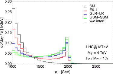
In this section we explore the role of interference on the observed FP. In Fig. 5(a), we show the same distribution as in Fig. 2(a) where, the histograms shown with a dashed line, correspond to the case where the interference interaction terms (between the $Z^{\prime}$ diagram and the $\gamma+Z$ ones) have been switched off in the MC event generator. Clearly the contribution of the interference is negligible and it does not affect the position of the FP.

(a) (b)

Figure 5: As in Fig. 2(a) with dashed lines representing (a) the case without the interference terms between the BSM and SM diagrams, and (b) the case of the pure $Z^{\prime}$ signal.

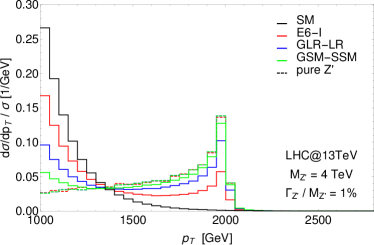
The same effect is visible in Fig. 5(b) where the dashed lines represent the $Z^{\prime}$ signal only, which has been determined by subtracting the SM background and its interference with the BSM signal. The presence and the position of the FP are once more unaffected by these changes: all the curves, representing either the full model or the pure $Z^{\prime}$ contribution, cross at the same point, demonstrating the stability of the FP manifestation. In conclusion, the FP position shows very little dependence on interference effects, further illustrating the model independent nature of this result.

II.3 The role of the width

We now consider the affect of varying the width on the FP. For this purpose, we focus on one specific benchmark, since similar results can be obtained in the other models. We show in Fig. 6 the binned distributions of the number of events as function of the lepton $p_{T}$ (a) and of the di-lepton system invariant mass (b) for the SSM model and different choices of the resonance width (1%, 5%, 10% and 20% of the mass) keeping the mass of the resonance fixed at 4 TeV. We stress again that in this analysis the width of the resonance has been enhanced by hand, that is the production cross section is unchanged, as well as the partial widths into the SM final states. The branching ratios however scales inversely with the width. This is representative of a scenario where extra decay channels are accessible to the neutral resonance, which is a very common picture in many BSM realisations predicting exotic matter.

(a) (b)

Figure 6: Distribution of number of events as function of (a) the $p_{T}$ of either lepton and (b) of the di-lepton invariant mass as predicted in the SM and in the SSM with $M_{Z^{\prime}}=4~{}{\rm TeV}$ at the 13 TeV LHC with $\mathcal{L}=1~{}ab^{-1}$. The width of the resonances has been fixed at four different values (1%, 5%, 10% and 20% of the mass). Acceptance cuts are applied ($|\eta|<2.5$), no detector efficiencies are accounted for.

Figure 7: Normalized distribution obtained from Fig. 6(a) with $p_{T}^{\rm min}=1000~{}GeV$.

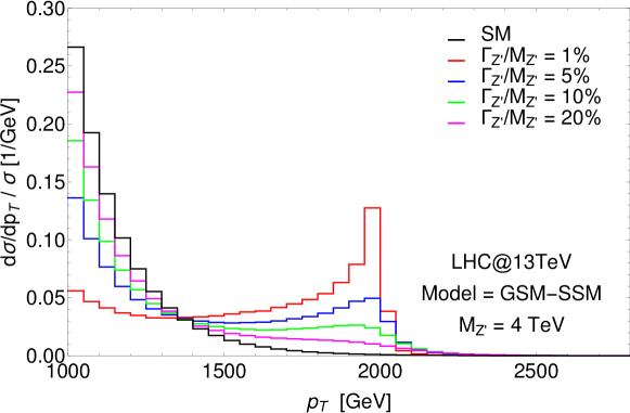
In Fig. 7 we illustrate the affect of different resonance width choices on the FP that appears after the usual normalisation procedure. The position of the FP can be seen to not depend on the resonance width. This is the key feature we exploit to define a new observable that can be used to constrain the resonance width.

II.4 The role of the mass

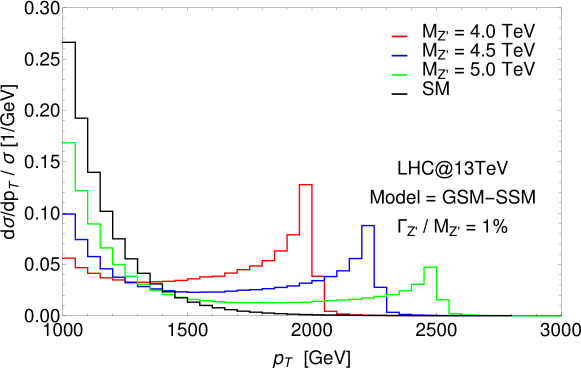
The effect of varying the $Z^{\prime}$ resonance mass is shown in the normalised pt distributions of Fig. 8. The SSM benchmark model is used where we constrain $\Gamma_{Z^{\prime}}/M_{Z^{\prime}}=1\%$. The position of the FP i.e. the intersection of the model curves with the SM background, does depend on $Z^{\prime}$ the mass as expected.

Figure 8: Normalised distribution in $p_{T}$ of either lepton as predicted in the SM and in in the SSM at the 13 TeV LHC. The mass of the resonances has been fixed at three different values (4.0, 4.5 and 5.0 TeV) while its width has been fixed at 1% of its mass. Acceptance cuts are applied ($|\eta|<2.5$), detector efficiencies are not accounted for.

II.5 The role of the low $p_{T}$ cut

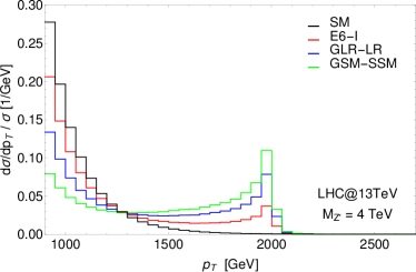
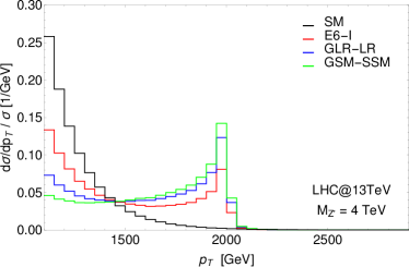
The main parameter affecting the FP position is, the choice of the low $p_{T}$ integration limit, which determines the curves’ normalisation factor. As shown in Fig. 9 the FP can be seen to change as a function of which low $p_{T}$ integration limit is applied. The two different $p_{T}$ choices in this figure can also be compared with the one in Fig. 2(a), where $p_{T}>1000$ GeV was chosen.

A correlation can be established between the FP location (for a given $Z^{\prime}$ mass and LHC energy) and the $p_{T}^{\rm min}$ cut used for the normalisation procedure. We have observed a numerical relation between the position of the FP and the choice of $p_{T}^{\rm min}$ and have heuristically determined that for the LHC at 13 TeV we can assume that the FP position (in GeV) is

$${\rm FP}[{\rm GeV}]\approx p_{T}^{\rm min}+10\%\;M_{Z^{\prime}}.$$ (II.1)

in the accessible range of $Z^{\prime}$ masses.

(a) (b)

Figure 9: Normalised distribution in $p_{T}$ of either lepton as predicted in the SM and in three $Z^{\prime}$ benchmark models with $M_{Z^{\prime}}=4~{}{\rm TeV}$ at the 13 TeV LHC. For all models the width of the resonance has been fixed at 1% of its mass. Acceptance cuts are applied ($|\eta|<2.5$), detector efficiencies are not accounted for. (a) $p_{T}^{\rm min}=900~{}{\rm GeV}$, (b) $p_{T}^{\rm min}=1100~{}{\rm GeV}$.

II.6 The role of the $\eta$ cut

For completeness, in this subsection we show the effect of a change in selection criterion in the lepton rapidity $\eta^{l}$. In Fig. 10 we have require($|\eta|<1.5$) for various choices of the low $p_{T}$ cut, to be compared with previous plots. No observable deviations from previous results are shown and the FP position does not change.

Figure 10: Normalised distribution in $p_{T}$ of either lepton as predicted in the SM and in three $Z^{\prime}$ benchmark models with $M_{Z^{\prime}}=4~{}$TeV. The width of the resonances has been fixed at 1% of their mass. The low $p_{T}$ cut for our choice of normalisation is $p_{T}^{\rm min}=1000~{}GeV$. Stronger than default acceptance cuts are applied for these plots ($|\eta|<1.5$), no detector efficiencies are accounted for though. Here, $\sqrt{s}=13$ TeV.

III Constraining $Z^{\prime}$ widths

In this section, we will show how the value of the intrinsic $Z^{\prime}$ width can be inferred from the use of a novel asymmetry observable based upon the concept of the FP, as discussed in the previous sections.

III.1 Defining a new observable: $A_{\rm FP}$

For a given collider energy and $Z^{\prime}$ mass, we have seen that suitably normalised single-lepton $p_{T}$ distributions for various $Z^{\prime}$ models all have the same magnitude at one point in the spectrum. We have dubbed this point the Focus Point. The $p_{T}$ value associated with it has been shown to not depend upon the intrinsic $Z^{\prime}$ width, in any of the models. For a fixed collider energy and a given $Z^{\prime}$ mass therefore, it is possible to define a unique FP that is common to a large class of models.

To define an observable based on the FP feature that can provide information about the width of the resonance we define two separate regions in the normalised $p_{T}$ distribution. The “Left” ($L$) region going from a fixed $p_{T}^{\rm min}$ (the low $p_{T}$ limit referred to above) up to the FP and the “Right” ($R$) region going from the FP up to the last point in the distribution, which we will assume is $p_{T}^{\rm max}>M_{Z^{\prime}}/2$.

We define an asymmetry around the FP, $A_{\rm FP}$, to be the difference between the integrated normalised distribution in the two regions, divided by the sum of the two integrations. This can be written

$$A_{\rm FP}=\frac{L-R}{L+R}$$ (III.1)

with

$$L=\frac{1}{N}\int_{L}\frac{d\sigma}{dp_{T}}dp_{T},\quad\quad R=\frac{1}{N}\int_{R}\frac{d\sigma}{dp_{T}}dp_{T},$$ (III.2)

where the two domains $L$ and $R$ are chosen as described above, i.e., $L=\left[p_{T}^{\rm min},{\rm FP}\right]$, $R=\left[{\rm FP},p_{T}^{\rm max}\right]$, with FP the FP position in the $p_{T}$ axis, and $N$ the total number of events in the $(L+R)$ region that we have also used for the normalization procedure. The expression we have derived for the new observable is notionally very similar to the Forward-Backward Asymmetry ($A_{\rm FB}$) Accomando et al. (2016a); Fiaschi et al. (2015); Accomando et al. (2015). In this sense, the formula for the statistical error on the $A_{\rm FP}$ observable is analogous to the one for the $A_{\rm FB}$, thus:

$$\Delta A_{\rm FP}=\sqrt{\frac{1-A_{\rm FP}^{2}}{N}},$$ (III.3)

This $A_{\rm FP}$ observable can be used to estimate the width of the $Z^{\prime}$ resonance, with the positive feature of being unbiased by systematics and assumptions intrinsic to shape dependent fitting procedures (such as assuming a Breit-Wigner resonance structure in the the di-lepton invariant mass spectrum) Thus, we are going to estimate the $A_{\rm FP}$ values for different $Z^{\prime}$ model and width choices, at the 13 TeV LHC for various $Z^{\prime}$ masses. At this point, it is important to mention that the definition of the $L$ and $R$ regions is crucial for a correct analysis of the results. The precise steps to follow are: (i) extraction of the mass of the resonance from the di-lepton invariant mass, possibly combined with the location of the maximum of the $p_{T}$ distribution (which roughly coincides with $M_{Z^{\prime}}/2$); (ii) definition of the FP position according to Eq. (II.1).

While $p_{T}^{\rm max}$ is essentially defined to be any point in transverse momentum past $M_{Z^{\prime}}/2$ (as seen in the various distributions that we have presented, the drop beyond this point is dramatic), we have some freedom in the choice of $p_{T}^{\rm min}$. For example, a high $p_{T}^{\rm min}$ would maximise the sensitivity to any BSM physics while a low $p_{T}^{\rm min}$ would maximise the sensitivity to different BSM scenarios. As discovery of some BSM physics is assumed to have already occurred from analysis of the $M_{ll}$ spectrum, for our purposes, a low $p_{T}^{\rm min}$ is indeed more appropriate.

In Tabs. 1–2 we show the calculated $A_{\rm FP}$ observable for the SM background and for the usual benchmark models assuming different widths. We consider two values for the $Z^{\prime}$ mass ($M_{Z^{\prime}}=4~{}{\rm TeV}$ and $M_{Z^{\prime}}=5~{}{\rm TeV}$) and three possible choices for the $p_{T}^{\rm min}$ for each mass. In general, as expected, as we move up the $p_{T}^{\rm min}$ (and consequently the FP location) we have more sensitivity to the presence of BSM physics while going in the opposite direction leads to an enhancement of the sensitivity to the $Z^{\prime}$ boson width.

The statistical errors are also reported in the two tables and they are obtained for an integrated luminosity of 1 and 3 ab^-1 respectively. The statistical error represents the dominant uncertainty in the $A_{\rm FP}$ observable. Being a ratio of cross sections systematic uncertainties are indeed expected to cancel partially. We give two examples of the expected size of the PDF uncertainty, to compare with the central value and the statistical error taken from Tab. 2.

$$M_{Z^{\prime}}=5~{}{\rm TeV},~{}\Gamma_{Z^{\prime}}/M_{Z^{\prime}}=5\%,~{}p_{T}^{\rm min}=1.2~{}{\rm TeV},$$

$$(A_{\rm FP}\pm\Delta_{\rm stat}\pm\Delta_{\rm PDF})_{\rm SM}=0.87\pm 0.07\pm 0.01,$$

$$(A_{\rm FP}\pm\Delta_{\rm stat}\pm\Delta_{\rm PDF})_{\rm SSM}=0.44\pm 0.12\pm 0.06.$$

$M_{Z^{\prime}}=4~{}{\rm TeV}$
Model	$\Gamma_{Z^{\prime}}/M_{Z^{\prime}}=1\%$	$\Gamma_{Z^{\prime}}/M_{Z^{\prime}}=5\%$	$\Gamma_{Z^{\prime}}/M_{Z^{\prime}}=10\%$	$\Gamma_{Z^{\prime}}/M_{Z^{\prime}}=20\%$
$p_{T}^{\rm min}=900~{}{\rm GeV}$
SM	0.82$\pm$0.05
$E_{6}^{I}$	0.44$\pm$0.07	0.72$\pm$0.06	0.77$\pm$0.06	0.80$\pm$0.06
LR	0.02$\pm$0.07	0.55$\pm$0.07	0.68$\pm$0.07	0.76$\pm$0.06
SSM	-0.29$\pm$0.05	0.26$\pm$0.08	0.50$\pm$0.08	0.67$\pm$0.07
$p_{T}^{\rm min}=1000~{}{\rm GeV}$
SM	0.81$\pm$0.08
$E_{6}^{I}$	0.27$\pm$0.10	0.65$\pm$0.09	0.72$\pm$0.09	0.77$\pm$0.08
LR	-0.14$\pm$0.07	0.40$\pm$0.10	0.58$\pm$0.10	0.70$\pm$0.09
SSM	-0.37$\pm$0.05	0.06$\pm$0.10	0.33$\pm$0.12	0.56$\pm$0.11
$p_{T}^{\rm min}=1100~{}{\rm GeV}$
SM	0.79$\pm$0.11
$E_{6}^{I}$	0.12$\pm$0.12	0.57$\pm$0.13	0.68$\pm$0.12	0.74$\pm$0.12
LR	-0.22$\pm$0.08	0.25$\pm$0.14	0.47$\pm$0.14	0.64$\pm$0.13
SSM	-0.38$\pm$0.05	-0.08$\pm$0.12	0.16$\pm$0.15	0.43$\pm$0.16

Table 1: $A_{\rm FP}$ and its statistical error for the SM and three benchmark models with $M_{Z^{\prime}}=4~{}{\rm TeV}$ and four different widths repeated for three choices of $p_{T}^{\rm min}$, for the LHC at 13 TeV and $\mathcal{L}=1~{}{\rm ab}^{-1}$. The FP position is obtained following Eq. II.1.

$M_{Z^{\prime}}=5~{}{\rm TeV}$
Model	$\Gamma_{Z^{\prime}}/M_{Z^{\prime}}=1\%$	$\Gamma_{Z^{\prime}}/M_{Z^{\prime}}=5\%$	$\Gamma_{Z^{\prime}}/M_{Z^{\prime}}=10\%$	$\Gamma_{Z^{\prime}}/M_{Z^{\prime}}=20\%$
$p_{T}^{\rm min}=1100~{}{\rm GeV}$
SM	0.88$\pm$0.05
$E_{6}^{I}$	0.71$\pm$0.07	0.84$\pm$0.06	0.85$\pm$0.05	0.87$\pm$0.05
LR	0.40$\pm$0.08	0.76$\pm$0.07	0.82$\pm$0.06	0.85$\pm$0.06
SSM	0.04$\pm$0.08	0.60$\pm$0.08	0.74$\pm$0.07	0.82$\pm$0.06
$p_{T}^{\rm min}=1200~{}{\rm GeV}$
SM	0.87$\pm$0.07
$E_{6}^{I}$	0.62$\pm$0.10	0.81$\pm$0.08	0.84$\pm$0.07	0.85$\pm$0.07
LR	0.22$\pm$0.10	0.68$\pm$ 0.10	0.77$\pm$0.09	0.83$\pm$0.08
SSM	-0.14$\pm$0.09	0.44$\pm$0.12	0.64$\pm$0.11	0.77$\pm$0.10
$p_{T}^{\rm min}=1300~{}{\rm GeV}$
SM	0.86$\pm$0.09
$E_{6}^{I}$	0.50$\pm$0.14	0.77$\pm$0.11	0.81$\pm$0.10	0.84$\pm$0.10
LR	0.06$\pm$0.12	0.58$\pm$0.14	0.72$\pm$0.13	0.80$\pm$0.11
SSM	-0.24$\pm$0.09	0.27$\pm$0.16	0.52$\pm$0.16	0.70$\pm$0.14

Table 2: $A_{\rm FP}$ and its statistical error for the SM and three benchmark models with $M_{Z^{\prime}}=5~{}{\rm TeV}$ and four different widths repeated for three choices of $p_{T}^{\rm min}$, for the LHC at 13 TeV and $\mathcal{L}=3~{}{\rm ab}^{-1}$. The FP position is obtained following Eq. II.1.

III.2 Sensitivity of the $A_{\rm FP}$ observable

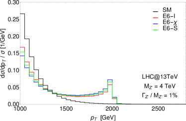
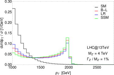
In this section we want to explore in more detail the potential of the new $A_{\rm FP}$ observable in discriminating amongst different $Z^{\prime}$ models. We begin by comparing BSM scenarios within the same class. We do so in Fig. 11, where we show the usual normalised $p_{T}$ distribution.

(a) (b)

Figure 11: Normalised distribution in $p_{T}$ of either lepton as predicted in the SM (black) and in three $Z^{\prime}$ benchmark models (coloured) within the $E_{6}$ class (a) and GLR and GSM classes (b) with $M_{Z^{\prime}}=4~{}$TeV and $p_{T}^{\rm min}=1000~{}GeV$. The width of the resonances has been fixed at 1% of their mass. Acceptance cuts are applied ($|\eta|<2.5$), no detector efficiencies are accounted for. Here, $\sqrt{s}=13$ TeV.

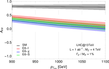
The distributions of the models in the $E_{6}$ class present clear similarities and the same behaviour is shown in the models belonging to the $LR$ class. In Fig. 12, we are showing the $A_{\rm FP}$ and its statistical error as function of the $p_{T}^{\rm min}$ cut.

(a) (b)

Figure 12: $A_{\rm FP}$ central value and statistical 1$\sigma$ error band as function of $p_{T}^{\rm min}$ for the LHC at 13 TeV and $\mathcal{L}=1~{}{\rm ab}^{-1}$. The black line represents the SM while the coloured lines represent three benchmark in the $E_{6}$ class (a) and GLR and GSM classes (b). The mass of the $Z^{\prime}$ boson is fixed at 4 TeV and its width has been fixed $\Gamma/M=1\%$. The values for the FPs are chosen in accordance to the tables above.

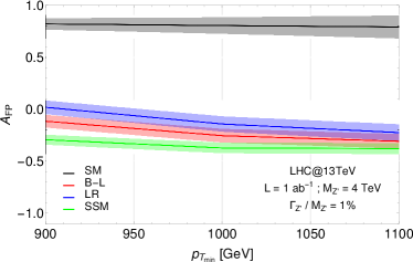
For what we can see, $Z^{\prime}$ models in the same class have similar values for $A_{\rm FP}$, all falling within the error bars already for $Z^{\prime}$ masses of 4 TeV and narrow resonances. This is definitely true for benchmarks in the $E_{6}$ class and a similar behaviour is shown for two GLR benchmarks as well ($LR$ and $B-L$). However, as the resonance mass or width increases, the differences between models tend to disappear. This, in essence, suggests that we cannot use this observable to discriminate between models within the same class.

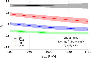
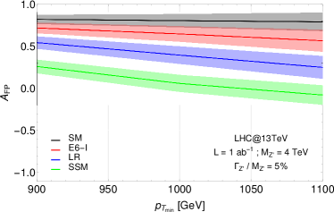
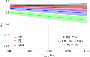
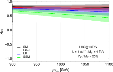
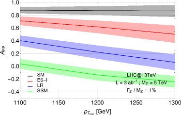
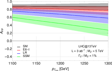
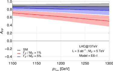
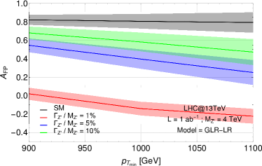
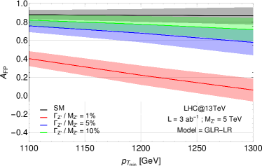
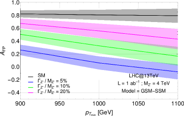
Still, we can exploit the discriminative power of $A_{\rm FP}$ against the SM background and amongst classes of models, ultimately extracting constraints that we can impose on the resonance width. With this is mind, we compare the $A_{\rm FP}$ predictions for the usual three classes of models for different widths, in Figs. 13–14, where we are showing $A_{\rm FP}$ and its statistical error for the three $Z^{\prime}$ benchmarks and SM as a function of $p_{T}^{\rm min}$ for two values of the resonance mass and different widths. As we can see, for a $Z^{\prime}$ boson mass around 4 TeV, the $A_{\rm FP}$ observable can distinguish between different models having $\Gamma_{Z^{\prime}}/M_{Z^{\prime}}\sim 10\%$ and in some cases up to 20% too. For a resonance mass around 5 TeV, instead, the sensitivity upon the different classes of models holds up to $\Gamma_{Z^{\prime}}/M_{Z^{\prime}}\sim 5\%$.

(a) (b) (c) (d)

Figure 13: $A_{\rm FP}$ central value and statistical 1$\sigma$ error band as function of $p_{T}^{\rm min}$ cut for the LHC at 13 TeV and $\mathcal{L}=1~{}{\rm fb}^{-1}$. The black line represents the SM while the coloured lines represent the three benchmark models. The mass of the $Z^{\prime}$ boson is fixed at 4 TeV while its width over mass ratio $\Gamma_{Z^{\prime}}/M_{Z^{\prime}}$ has been fixed to 1% (a), 5% (b), 10% (c) and 20% (d). The values for the FP are chosen in accordance to the tables above.

(a) (b)

Figure 14: $A_{\rm FP}$ central value and statistical 1$\sigma$ error band as function of $p_{T}^{\rm min}$ cut for the LHC at 13 TeV and $\mathcal{L}=3~{}{\rm ab}^{-1}$. The black line represents the SM while the coloured lines represent the three benchmark models. The mass of the $Z^{\prime}$ boson is fixed at 5 TeV while its width over mass ratio $\Gamma_{Z^{\prime}}/M_{Z^{\prime}}$ has been fixed to 1% (a) and 5% (b). The values for the FP are chosen in accordance to the tables above.

(a) (b) (c) (d) (e) (f)

Figure 15: $A_{\rm FP}$ central value and statistical 1$\sigma$ error band as function of $p_{T}^{\rm min}$ cut for the LHC at 13 TeV and $\mathcal{L}=1~{}{\rm ab}^{-1}$. The black line represents the SM while the coloured lines represent four different widths (1%, 5%, 10% and 20%) of the $Z^{\prime}$ resonance in the $E_{6}^{I}$ (a), $LR$ (c) and SSM (e) model with a mass of the $Z^{\prime}$ boson fixed at 4 TeV. The values for the FP are chosen in accordance to the tables above. Similarly we repeat the same exercise for the $E_{6}^{I}$ (b), $LR$ (d) and SSM (f) model with a mass of the $Z^{\prime}$ boson fixed at 5 TeV and and $\mathcal{L}=3~{}{\rm ab}^{-1}$.

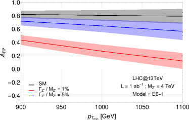
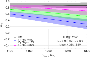
Finally, coming back to our original purpose, we want to discuss now the sensitivity of $A_{\rm FP}$ upon the resonance width. In Figs. 15 we are showing its discriminative power against the resonance width within each class for two choices of the $Z^{\prime}$ boson mass. The $A_{\rm FP}$ observable seems to fulfil the task: within each class of models we are able to set important constraints on the resonance width. In the case of resonances of the order of 4 TeV, assuming an integrated luminosity of 1 ab^-1, we would be able to constrain their widths up to $\Gamma_{Z^{\prime}}/M_{Z^{\prime}}\sim 5\%$ within the $E_{6}$ class of models, up to $\Gamma_{Z^{\prime}}/M_{Z^{\prime}}\sim 10\%$ within the $LR$ class of models and up to $\Gamma_{Z^{\prime}}/M_{Z^{\prime}}\sim 20\%$ within the $SSM$ class of models For resonances of the order of 5 TeV we obtain similar results, assuming an integrated luminosity of 3 ab^-1.

IV Conclusions

In summary, we have defined a new kinematic asymmetry, $A_{\rm FP}$, based around a FP appearing in the normalised transverse momentum distribution of either lepton in DY processes. The remarkable features of this FP are its insensitivity to the underlying $Z^{\prime}$ model as well as quantities which carry (theoretical) systematic errors such as PDFs and their factorisation and renormalisation scales. Hence, this FP displays model-independent characteristics, as it is only sensitive to the collider energy (which is known) and the mass of the intervening $Z^{\prime}$ (which is expected to be extracted from the di-lepton invariant mass).

In fact, while the FP location is stable against variations of the $Z^{\prime}$ boson width, the $A_{\rm FP}$ asymmetry strongly dependent upon the width. The combination of these features makes of $A_{\rm FP}$ a suitable observable to determine the characteristics of any $Z^{\prime}$ which may be discovered at the LHC. Lastly, the $A_{\rm FP}$ could also be used to limit the possible range of widths of a $Z^{\prime}$ signal which could be used as a constraint in a fit of a resonance peak in an invariant mass spectrum.

Finally, we remark that the effectiveness of the new variable will increase significantly with the LHC luminosity, so as to expect that its importance will be appreciated after a few years of Run 2 (i.e., after some 300 fb^-1 of data) or else rather immediately at a future High-Luminosity LHC (HL-LHC) stage Gianotti et al. (2005) (i.e., starting from 1 ab^-1 of data), depending on the $Z^{\prime}$ mass, width and couplings.

References

- Accomando et al. (2011) E. Accomando, A. Belyaev, L. Fedeli, S. F. King, and C. Shepherd-Themistocleous, Phys.Rev. D83, 075012 (2011), arXiv:1010.6058 [hep-ph] .
- Belyaev et al. (2009) A. Belyaev, R. Foadi, M. T. Frandsen, M. Jarvinen, F. Sannino, and A. Pukhov, Phys. Rev. D79, 035006 (2009), arXiv:0809.0793 [hep-ph] .
- Barducci et al. (2013) D. Barducci, A. Belyaev, S. De Curtis, S. Moretti, and G. M. Pruna, JHEP 1304, 152 (2013), arXiv:1210.2927 [hep-ph] .
- Kim and Lee (2014) Y. G. Kim and K. Y. Lee, Phys. Rev. D90, 117702 (2014), arXiv:1405.7762 [hep-ph] .
- Malkawi and Yuan (2000) E. Malkawi and C. P. Yuan, Phys. Rev. D61, 015007 (2000), arXiv:hep-ph/9906215 [hep-ph] .
- Altarelli et al. (1989) G. Altarelli, B. Mele, and M. Ruiz-Altaba, Z.Phys. C45, 109 (1989).
- Accomando et al. (2013) E. Accomando, D. Becciolini, A. Belyaev, S. Moretti, and C. Shepherd-Themistocleous, JHEP 1310, 153 (2013), arXiv:1304.6700 [hep-ph] .
- Collaboration (2016) C. Collaboration (CMS), (2016).
- collaboration (2017) T. A. collaboration (ATLAS), (2017).
- Accomando et al. (2016a) E. Accomando, A. Belyaev, J. Fiaschi, K. Mimasu, S. Moretti, and C. Shepherd-Themistocleous, JHEP 01, 127 (2016a), arXiv:1503.02672 [hep-ph] .
- Balossini et al. (2008) G. Balossini, G. Montagna, C. M. Carloni Calame, M. Moretti, M. Treccani, O. Nicrosini, F. Piccinini, and A. Vicini, Proceedings, 14th Cracow Epiphany Conference on LHC Physics: Cracow, Poland, January 4-6, 2008, Acta Phys. Polon. B39, 1675 (2008), arXiv:0805.1129 [hep-ph] .
- Li and Petriello (2012) Y. Li and F. Petriello, Phys. Rev. D86, 094034 (2012), arXiv:1208.5967 [hep-ph] .
- Dulat et al. (2016) S. Dulat, T.-J. Hou, J. Gao, M. Guzzi, J. Huston, P. Nadolsky, J. Pumplin, C. Schmidt, D. Stump, and C. P. Yuan, Phys. Rev. D93, 033006 (2016), arXiv:1506.07443 [hep-ph] .
- Accomando et al. (2016b) E. Accomando, J. Fiaschi, F. Hautmann, S. Moretti, and C. H. Shepherd-Themistocleous, (2016b), arXiv:1606.06646 [hep-ph] .
- Fiaschi et al. (2015) J. Fiaschi, E. Accomando, A. Belyaev, K. Mimasu, S. Moretti, and C. H. Shepherd-Themistocleous, Proceedings, 2015 European Physical Society Conference on High Energy Physics (EPS-HEP 2015), PoS EPS-HEP2015, 176 (2015), arXiv:1510.05892 [hep-ph] .
- Accomando et al. (2015) E. Accomando, A. Belyaev, J. Fiaschi, K. Mimasu, S. Moretti, et al., (2015), arXiv:1504.03168 [hep-ph] .
- Gianotti et al. (2005) F. Gianotti et al., Eur. Phys. J. C39, 293 (2005), arXiv:hep-ph/0204087 [hep-ph] .