Adiabatic self-consistent collective path in nuclear fusion reactions

Abstract

Collective reaction paths for fusion reactions, ¹⁶O+$\alpha$ $\rightarrow$ ²⁰Ne and ¹⁶O+¹⁶O $\rightarrow$ ³²S, are microscopically determined, on the basis of the adiabatic self-consistent collective coordinate (ASCC) method. The collective path is maximally decoupled from other intrinsic degrees of freedom. The reaction paths turn out to deviate from those obtained with standard mean-field calculations with constraints on quadrupole and octupole moments. The potentials and inertial masses defined in the ASCC method are calculated along the reaction paths, which leads to the collective Hamiltonian used for calculation of the sub-barrier fusion cross sections. The inertial mass inside the Coulomb barrier may have a significant influence on the fusion cross section at the deep sub-barrier energy.

I Introduction

The microscopic description of the large amplitude nuclear collective motion is one of the major and long-standing problems in nuclear physics. For the collective motion in a complex multinucleon system, it is useful to describe its dynamics in terms of a small number of collective coordinates $q$. In most cases, one “intuitively” adopts deformation parameters $q$, such as the intrinsic quadrupole moment. In the energy density functional (EDF) approaches Schunck and Robledo (2016), a collective subspace (path) $|\psi(q)\rangle$ is constructed by performing the constrained minimization calculation with one-body constraining operators associated with those deformation parameters. Even simpler methods could be adopted, by assuming a single-particle potential, such as the Nilsson potential, as a function of the deformation parameters Brack et al. (1972). It is certainly desirable to microscopically extract a few collective variables, without relying on our intuitive choice, which are maximally decoupled from all the other intrinsic degrees of freedom.

The most well-known theory for this purpose, to determine such an optimal collective subspace, is the adiabatic time-dependent Hartree-Fock (ATDHF) theory Brink et al. (1976); Villars (1977); Baranger and Vénéroni (1978); Goeke and Reinhard (1978). The ATDHF theory is derived by using the expansion with respect to collective momenta $p$ up to the first order. In practical calculations, the ATDHF is formulated into the form of differential equation with initial states. Starting from different initial conditions, the ATDHF equation produces different collective paths. Many trajectories must be produced to find the “best” one Goeke et al. (1983); Reinhard and Goeke (1987). This is known as a “non-uniqueness” problem. A possible way to overcome this problem is to take into account the second-order terms in momentum $p$ Mukherjee and Pal (1982); Dang et al. (2000).

The adiabatic self-consistent collective coordinate (ASCC) method provides us an alternative approach, free from the non-uniqueness problem, to determining the optimal collective path or a collective sub-manifold embedded in the large-dimensional phase space of Slater determinants Matsuo et al. (2000); Nakatsukasa et al. (2016). The ASCC method has been applied to nuclear structure problems Hinohara et al. (2008, 2009, 2010, 2011, 2012); Sato et al. (2012); Matsuyanagi et al. (2016); Nakatsukasa (2012). In Ref. Wen and Nakatsukasa (2016), we have proposed a numerical method to solve the ASCC equations for nuclear reaction, combining the imaginary-time evolution Davies et al. (1980) and the finite amplitude method Nakatsukasa et al. (2007a); Avogadro and Nakatsukasa (2011a, 2013a). The test calculation has been done for the simplest system of the reaction path of $\alpha$+$\alpha$ $\rightarrow$ ⁸Be. The present paper is on the continuation of this work. The numerical methods proposed in Ref. Wen and Nakatsukasa (2016) are applied to nuclear fusion reactions of ¹⁶O+$\alpha$ $\rightarrow$ ²⁰Ne and ¹⁶O+¹⁶O $\rightarrow$ ³²S. They demonstrate unique features of the collective dynamics, showing that the optimal collective path can be different from the constrained Hartree-Fock (CHF) states with constraints on the mass quadrupole and octupole moments.

The inertial mass is another important issue in nuclear collective motion. The ASCC method is capable of providing the masses for the collective motion in the decoupled subspace including effects of time-odd mean fields. They are different from other known inertial masses, such as those of the gaussian overlap approximation for the generator coordinate method and the cranking formula Ring and Schuck (1980). We will show significant difference between the ASCC and the cranking formulae, especially inside the Coulomb barrier.

The paper is organized as follows. In Sec. II, we give the formulation of the basic ASCC equations, to determine the collective path and to calculate the mass parameter. In Sec. III, we apply the method to extract the collective paths for the reaction systems of ¹⁶O+$\alpha$ $\rightarrow$ ²⁰Ne and ¹⁶O+¹⁶O $\leftrightarrow$ ³²S. The inertial mass with respect to the relative distance between two nuclei are calculated. The sub-barrier fusion cross section is estimated from the results. Summary and concluding remarks are given in In Sec. IV

II Theoretical framework

In this section, we recapitulate the basic formulation of the ASCC method without the pairing correlation. Then, we briefly describe a procedure to construct the one-dimensional (1D) collective path and to calculate the inertial mass. The details can be found in Ref. Wen and Nakatsukasa (2016).

II.1 Basic equations of the ASCC method

In the present study, we assume that the reaction is described by the 1D collective coordinate $q(t)$ and its conjugate momentum $p(t)$. Parameterizing the time-dependent mean-field states (Slater determinants) as $|{\psi(p,q)}\rangle$, the total energy of the system in this parametrization reads

$$H(p,q)=\langle\psi(p,q)|\hat{H}|\psi(p,q)\rangle,$$ (1)

which defines a classical collective Hamiltonian. In the ASCC method, the optimal collective path $|{\psi(p,q)}\rangle$ is obtained so as to be maximally decoupled from the intrinsic degrees of freedom. Therefore, the evolution of $q(t)$ and $p(t)$ approximately obey the canonical equation of motion with the Hamiltonian $H(p,q)$.

The state $|{\psi(p,q)}\rangle$ is written in powers of $p$ about $p=0$ as

$$|\psi(p,q)\rangle=e^{ip\hat{Q}(q)}|\psi(0,q)\rangle=e^{ip\hat{Q}(q)}|{\psi(q)}\rangle,$$ (2)

where $\hat{Q}(q)$ is defined as $\hat{Q}(q)|\psi(q)\rangle=-i\partial_{p}|\psi(q)\rangle$. The conjugate operator $\hat{P}(q)$ is introduced as an infinitesimal generator for translating the system with respect to $q$, $\hat{P}(q)|\psi(q)\rangle=i\partial_{q}|\psi(q)\rangle$. $\hat{P}(q)$ and $\hat{Q}(q)$ can be expressed in the form of one-body operator as

$$\hat{P}(q) = i\sum_{n\in p,j\in h}P_{nj}(q)a^{{\dagger}}_{n}(q)a_{j}(q)+\mathrm{h.c.},$$ (3)

$$\hat{Q}(q) = \sum_{n\in p,j\in h}Q_{nj}(q)a^{{\dagger}}_{n}(q)a_{j}(q)+\mathrm{h.c.}.$$ (4)

They are locally defined at each $q$ and change their structure along the collective path. The particle ($n\in p$) and hole ($j\in h$) states are also defined with respect to $|{\psi(q)}\rangle$. The weak canonicity condition

$$\langle\psi(q)|[i\hat{P}(q),\hat{Q}(q)]|\psi(q)\rangle=1$$ (5)

is imposed to make $q$ and $p$ a pair of canonical variables.

The self-consistent collective coordinate (SCC) method is based on the invariance principle of the time-dependent mean-field theory Marumori et al. (1980). The adiabatic approximation in ASCC refers to the assumption that the collective momentum $p$ is small, so that we can expand equations in terms of $p$ up to the order of $p^{2}$. The invariance principle of SCC leads to the following set of ASCC equations Matsuo et al. (2000); Nakatsukasa et al. (2016),

$$\delta\langle{\psi(q)}|\hat{H}_{\rm mv}(q)|{\psi(q)}\rangle=0$$ (6)

$$\delta\langle\psi(q)|[\hat{H}_{\rm mv}(q),\frac{1}{i}\hat{P}(q)]-\frac{\partial^{2}V}{\partial q^{2}}\hat{Q}(q)|\psi(q)\rangle=0,$$ (7)

$$\delta\langle\psi(q)|[\hat{H}_{\rm mv}(q),i\hat{Q}(q)]-\frac{1}{M(q)}\hat{P}(q)|\psi(q)\rangle=0,$$ (8)

where $\hat{H}_{\rm mv}(q)\equiv\hat{H}-(\partial V/\partial q)\hat{Q}(q)$ is the “moving” Hamiltonian. Here, the curvature term, associated with $d\hat{Q}/dq$, is neglected for simplicity Nakatsukasa et al. (2016). The collective potential $V(q)$ is defined as

$$V(q)=\langle\psi(q)|\hat{H}|\psi(q)\rangle,$$ (9)

and $M(q)$ is the inertial mass of the collective motion. Equation (6) is called “moving mean-field equation” (“moving Hartree-Fock (HF) equation”), and Eqs. (7) and (8) are “moving random-phase approximation (RPA)”. This set of equations determines the reaction path $|{\psi(q)}\rangle$ as well as the local generators, $\hat{P}(q)$ and $\hat{Q}(q)$, self-consistently.

To fix the scale of $\hat{P}(q)$ and $\hat{Q}(q)$, for the present study, we set the mass $M(q)$ in Eq. (8) to be a constant value, $M(q)=M_{q}=1\ \hbar^{2}$MeV^-1fm^-2. This determines the scale and the dimension of the coordinate $q$. The second order derivative of the potential energy with respect to $q$ corresponds to the squared frequency of the moving RPA.

$$\omega^{2}(q)=\frac{1}{M_{q}}\frac{\partial^{2}V}{\partial q^{2}}.$$ (10)

To solve the moving RPA equations (7) and (8), we make use of the the finite amplitude method (FAM)  Nakatsukasa et al. (2007b); Avogadro and Nakatsukasa (2011b), especially the matrix FAM prescription Avogadro and Nakatsukasa (2013b). In the FAM, only the calculations of the single-particle Hamiltonian constructed with independent bra and ket states are required  Nakatsukasa et al. (2007b), providing us a high numerical efficiency to solve Eqs. (7) and (8). The moving mean-field equation (6) is solved by using the imaginary-time method. In practical calculation, we adopt the coordinate-space representation for the mean-field states and the mixed representation for the RPA matrix Wen and Nakatsukasa (2016).

II.2 Construction of collective reaction path

We may start the construction of the collective path, in principle, from any state $|{\psi(q)}\rangle$ that satisfies Eqs. (6), (7), and (8). There are a kind of “trivial” states; the ground state of the whole system (after fusion) and the state with well separated projectile and target (before fusion). We start the construction procedure from one of these trivial initial states. At the initial state $|{\psi(q=0)}\rangle$ on the collective path, the solutions of the moving RPA equations (7) and (8) provide many kinds of modes, among which we need to select the one associated with the reaction path. Here, we choose the lowest mode of excitation except for the Nambu-Goldstone (NG) modes associated with the translation and rotation of the total system.

To identify character of the modes, we calculate the transition strength of multipole operators.

$$\hat{Q}_{LK}\equiv\sum_{q=n,p}\sum_{s=\pm 1/2}\int r^{l}Y_{LK}(\hat{r})\hat{\psi}_{sq}^{\dagger}(\vec{r})\hat{\psi}_{sq}(\vec{r})d\vec{r}.$$ (11)

The magnetic quantum number $K$ is defined with respect to the axis of deformation. Each RPA mode has the eigenfrequency $\omega$ and the generators $\hat{P}(q=0)$ and $\hat{Q}(q=0)$. Taking a suitable linear combination of $\hat{Q}_{LK}$ and $\hat{Q}_{L-K}$, we can make $\hat{Q}_{LK}$ hermitian with real matrix elements. The transition strengths between the RPA ground state $|{0}\rangle$ and excited state $|{\omega}\rangle$ are calculated as

$$\langle{\omega}|\hat{Q}_{LK}|{0}\rangle=\sqrt{\frac{1}{2\omega}}\sum_{n\in p,j\in h}(Q_{LK})_{nj}P_{nj},$$ (12)

where $(Q_{LK})_{nj}$ are the ph matrix elements of $\hat{Q}_{LK}$. The NG modes are characterized by the zero energy ($\omega=0$) and by large matrix elements of $Q_{LK}$ with $L=1$ (translation) and the $(L,K)=(2,\pm 1)$ (rotation). In contrast, the reaction path is associated with large transition strength for $\hat{Q}_{20}$ and/or $\hat{Q}_{30}$. Moving away from the initial state, we choose a set of generators $(\hat{Q}(q),\hat{P}(q))$, using a condition that the generators must continuously change.

Next we show how to construct the collective path Wen and Nakatsukasa (2016). Although fully self-consistent solution of the moving HF equation (6) is possible, it is significantly facilitated by adopting an approximation, $\hat{Q}(q+\delta q)\approx\hat{Q}(q)$. Since $\hat{Q}(q)$ is a smooth function of $q$, this is reasonable for a small step size $\delta q$. Thus, the moving Hamiltonian at $q+\delta q$ is now given by $\hat{H}_{\rm mv}(q+\delta q)=\hat{H}-\lambda\hat{Q}(q)$. The Lagrange multiplier $\lambda$ is determined by the constraint on the step size,

$$\langle{\psi(q+\delta q)}|\hat{Q}(q)|{\psi(q+\delta q)}\rangle=\delta q.$$ (13)

In this way, the system moves from $|{\psi(q)}\rangle$ to $|{\psi(q+\delta q)}\rangle$, obtaining a new state $|{\psi(q+\delta q)}\rangle$ on the collective path.

Solving Eqs. (7) and (8) at $|{\psi(q+\delta q)}\rangle$, the generators are updated from $\hat{Q}(q)$ to $\hat{Q}(q+\delta q)$. Then, we can construct the next state, $|{\psi(q+2\delta q)}\rangle$. Continuing this iteration, we will obtain a series of states, $|{\psi(q=0)}\rangle$, $|{\psi(\delta q)}\rangle$, $|{\psi(2\delta q)}\rangle$, $|{\psi(3\delta q)}\rangle,\cdots$, forming a collective path. In this work, we set $\delta q$ within the magnitude of 0.1 fm in Eq. (13). In order to check the validity of the approximation $\hat{Q}(q+\delta q)=\hat{Q}(q)$ at any $q$, we perform the imaginary-time evolution for the obtained $|{\psi(q)}\rangle$ with $\hat{H}_{\rm mv}(q)=\hat{H}-\lambda\hat{Q}(q)$, and confirm that the state is almost invariant under the iteration.

We should remark a practical treatment of the NG modes. In principle, the ASCC guarantees the separation of the NG modes from other normal modes Matsuo et al. (2000); Nakatsukasa et al. (2016). However, in this study, we neglect the curvature term in Eq. (8). Thus, at a non-equilibrium point $|{\psi(q)}\rangle$ away from the ground state, they can mix with other physical modes of excitation. Furthermore, in practice, because of the finite mesh size for the grid representation of the coordinate space (Sec. III), the exact translational and rotational symmetries are violated. This is not a problem, if the system has certain symmetries which prohibit a mixture of the NG modes with physical modes of interest. For instance, the collision of two ¹⁶O nuclei is free from the problem, because the system keeps the parity and the axial symmetry, thus, the $K^{\pi}$ quantum numbers clearly separate the NG modes from the colliding motion of two nuclei. In contrast, for the asymmetric reaction of $\alpha+^{16}$O, the NG mode corresponding to the translation of the center of mass along the symmetric axis can be mixed with the $K^{\pi}=0^{-}$ excitation. In this case we need to remove the NG components ($\hat{Q}^{\rm NG}(q),\hat{P}^{\rm NG}(q)$) from the ASCC generators, $\hat{Q}^{\rm cal}(q)$ and $\hat{P}^{\rm cal}(q)$. Since the NG generators $(\hat{Q}^{\rm NG},\hat{P}^{\rm NG})$ are trivially obtained in the translational motion, the ASCC generators for the reaction are easily corrected as

$$\hat{Q}(q) = \hat{Q}^{\rm cal}(q)-\lambda^{Q}_{q}\hat{Q}^{\rm NG}-\lambda^{Q}_{p}\hat{P}^{\rm NG},$$ (14)

$$\hat{P}(q) = \hat{P}^{\rm cal}(q)-\lambda^{P}_{q}\hat{Q}^{\rm NG}-\lambda^{P}_{p}\hat{P}^{\rm NG},$$ (15)

with

$$\lambda^{Q}_{q} = -i\langle{\psi(q)}|[\hat{Q}^{\rm cal},\hat{P}^{\rm NG}|{\psi(q)}\rangle,$$ (16)

$$\lambda^{Q}_{p} = i\langle{\psi(q)}|[\hat{Q}^{\rm cal},\hat{Q}^{\rm NG}|{\psi(q)}\rangle,$$ (17)

$$\lambda^{P}_{q} = -i\langle{\psi(q)}|[\hat{P}^{\rm cal},\hat{P}^{\rm NG}|{\psi(q)}\rangle,$$ (18)

$$\lambda^{P}_{p} = i\langle{\psi(q)}|[\hat{P}^{\rm cal},\hat{Q}^{\rm NG}|{\psi(q)}\rangle,$$ (19)

which can be derived from the condition, $[\hat{Q}(q),\hat{Q}^{\rm NG}]=[\hat{Q}(q),\hat{P}^{\rm NG}]=[\hat{P}(q),\hat{Q}^{\rm NG}]=[\hat{P}(q),\hat{P}^{\rm NG}]=0$.

II.3 Inertial mass for nuclear reaction

As mentioned in Sec. II.1, to fix the arbitrary scale of $q$, the inertial mass $M(q)$ with respect to $q$ in Eq. (8) is set to be 1 $\hbar^{2}$MeV^-1fm^-2. In order to obtain a physical picture of the collective dynamics, it is convenient to label the collective path by other coordinates intuitively chosen by ourselves. For instance, in the asymptotic region where the two colliding nuclei are well apart, it is natural to adopt the relative distance $R$ between projectile and target. As far as the one-to-one correspondence between $q$ and $R$ is guaranteed, we may use the mapping function $R(q)$ to modify the scale of the coordinate, without losing anything. For the coordinate $R$, the inertial mass should be transformed as

$$M(R)=M_{q}\left(\frac{dq}{dR}\right)^{2}=M_{q}\left(\frac{dR}{dq}\right)^{-2}.$$ (20)

Thus, the mass $M(R)$ requires the calculation of the derivative $dR/dq$, which can be obtained as

$$\frac{dR}{dq} = \frac{d}{dq}\langle\psi(q)|\hat{R}|\psi(q)\rangle=\langle\psi(q)|[\hat{R},\frac{1}{i}\hat{P}(q)]|\psi(q)\rangle$$ (21)

$$= 2\sum_{n\in p,j\in h}R_{nj}(q)P_{nj}(q),$$

with the local generator $\hat{P}(q)$. $R_{nj}(q)$ are the ph matrix elements of $\hat{R}$.

In this paper, the one-body operator $\hat{R}$ for the relative distance between projectile and target is defined as follows. Assuming the relative motion along z axis with projectile on the right and target on the left, we introduce a separation plane at $z=z_{\rm s}$ so that

$$\int_{-\infty}^{\infty}dx\int_{-\infty}^{\infty}dy\int_{z_{\rm s}}^{+\infty}dz\rho(\vec{r})=A_{\rm pro},$$ (22)

where $\rho(\vec{r})$ is the total density, $A_{\rm pro}$ ($A_{\rm tar}$) is the mass number of the projectile (target). The operator form of $R$ reads

$$\hat{R}\equiv\sum_{s,q}\int d\vec{r}\hat{\psi}_{sq}^{\dagger}(\vec{r})\hat{\psi}_{sq}(\vec{r})z\left[\frac{\theta(z-z_{\rm s})}{A_{\rm pro}}-\frac{\theta(z_{\rm s}-z)}{A_{\rm tar}}\right],$$ (23)

where $\theta$ is the step function. For the symmetric reaction system, the section plane is at $z_{\rm s}=0$. $\hat{R}$ reduces to

$$\hat{R}=\frac{2}{A}\sum_{s,q}\int d\vec{r}z\hat{\psi}_{sq}^{\dagger}(\vec{r})\hat{\psi}_{sq}(\vec{r})\left[\theta(z)-\theta(-z)\right].$$ (24)

III Applications

In this section we present results of numerical application to the fusion reaction. We employ the Bonche-Koonin-Negele (BKN) EDF Bonche et al. (1976), which assumes the spin-isospin symmetry without the spin-orbit interaction. To express the orbital wave functions, the grid representation is employed, discretizing the rectangular box into the three-dimensional (3D) Cartesian mesh. The model space is set to be $12\times 12\times 18$ fm³ for the reaction ¹⁶O+$\alpha$ $\rightarrow$ ²⁰Ne, $12\times 12\times 24$ fm³ for the system ¹⁶O+¹⁶O $\rightarrow$ ³²S, the mesh size is set to be 1.1 fm.

III.1 ¹⁶O+$\alpha$ $\rightarrow$ ²⁰Ne

III.1.1 Collective path: ¹⁶O$+\alpha\rightarrow$ ground-state ²⁰Ne

As a trivial solution of the ASCC equations, the well separated ¹⁶O and $\alpha$ both at the ground states can be the initial state $|\psi(q=0)\rangle$ to start the iterative procedure in Sec. II.2. Alternatively the ground state of ²⁰Ne can also be the initial state for the iteration. Although it is not trivial, we find that the same trajectory is produced starting from these two initial states. The ASCC collective path smoothly connects the two well separated nuclei, ¹⁶O and $\alpha$, to ²⁰Ne at ground state. The ground state of ²⁰Ne has a large quadrupole deformation. The density profile is shown in Fig. 1 (d). At the ground state, the lowest physical RPA state is found to be the $K^{\pi}=0^{-}$ octupole excitation, which has a sizable transition strength of the operator $\hat{Q}_{30}$ defined in Eq. (11). Choosing this $K^{\pi}=0^{-}$ octupole mode as the generators $\hat{Q}(q)$ and $\hat{P}(q)$, a series of states can be obtained by iteration, forming a collective fusion path of ¹⁶O+$\alpha$ $\leftrightarrow$ ²⁰Ne. In the asymptotic region (Fig.  1 (a)), the generators smoothly change into those representing the relative motion between ¹⁶O and $\alpha$. Figure 1 shows density distributions in the x-z plane ($y=0$) at four different points on the collective path. The panel (a) shows the well separated ¹⁶O + $\alpha$, the panel (d) shows ²⁰Ne at ground state, and two intermediate states are shown in the panels (b) and (c).

Figure 1: (Color online) Density distribution on the x-z plane at four points on the ASCC fusion reaction path of ¹⁶O + $\alpha\rightarrow^{20}$Ne: (a) $R=7.6$ fm, (b) $R=5.2$ fm, (c) $R=4.2$ fm, and (d) $R=3.8$ fm corresponding to the ground state of ²⁰Ne.

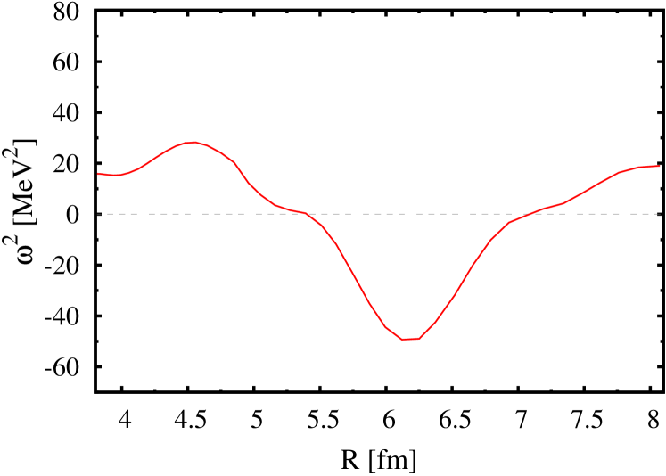
Figure 2: (Color online) Square of the moving RPA eigenfrequency $\omega^{2}(q)$ on the ASCC collective path of ¹⁶O + $\alpha\rightarrow^{20}$Ne, shown as a function of relative distance $R$. At the ground state of ²⁰Ne ($R=3.8$ fm), this mode corresponds to the $K^{\pi}=0^{-}$ octupole mode of excitation.

Figure 2 shows the square of moving RPA eigenfrequency $\omega^{2}(q)$ of the generators with $K=0$, as a function of relative distance $R$. At the ground state of ²⁰Ne ($R=3.8$ fm), the parity is a good quantum number and the RPA mode corresponds to the negative parity $\pi=-$, leading to $\langle{\omega}|\hat{Q}_{30}|{0}\rangle=3017$ fm³ and $\langle{\omega}|\hat{Q}_{20}|{0}\rangle=0$. At larger $R$, the octupole deformation $Q_{30}$ increases, then, the parity is no longer conserved. The transition strength $\langle{\omega}|\hat{Q}_{20}|{0}\rangle$ becomes nonzero, then, gradually changes its character into the relative motion between ¹⁶O and $\alpha$. Since the curvature of the potential energy can be negative, the value of $\omega^{2}(q)$ can be negative leading to imaginary $\omega(q)$. Since the generators keep the $K=0$ character all the way, the states $|{\psi(q)}\rangle$ on the collective path are axially symmetric. There appear five NG modes, namely, two rotational modes, and the three translational modes. In actual calculation, these NG modes have finite energy due to the finite mesh size in numerical calculation. At the ground state, we obtain $\omega=1.9$ MeV for the rotational modes, $\omega=3.5$ MeV for the translational modes along x and y directions, and $\omega=1.3$ MeV for the translational mode along z direction.

The next lowest $K=0$ mode of excitation at the ground state of ²⁰Ne has the positive parity $\pi=+$ and a transition strength of operator of $\hat{Q}_{20}$, $\langle{\omega}|\hat{Q}_{20}|{0}\rangle=5.3$ fm². The RPA frequency $\omega$ of this state is about 10 MeV, which is much higher than the octupole mode and many other modes with $K\neq 0$. If we adopt this $K^{\pi}=0^{+}$ mode as the starting generators, we cannot construct the collective path connecting the ground state and two separated nuclei. Generally speaking, the higher the RPA eigenfrequency is, the more difficult it is to find a solution of the moving mean-field equation (6).

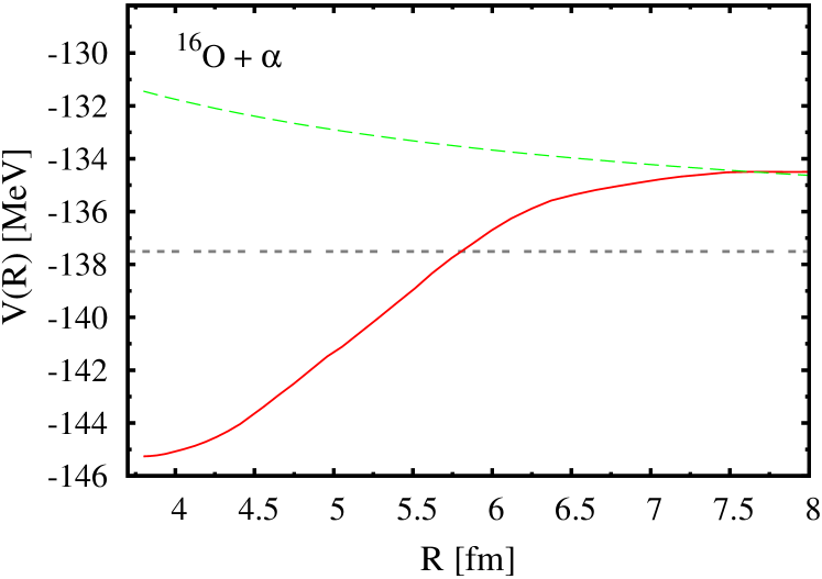
Figure 3: (Color online) Potential energy for the fusion path ¹⁶O + $\alpha\rightarrow^{20}$Ne as a function of relative distance $R$. The solid (red) line corresponds to $V(R)$ on the ASCC collective path, while the dashed (green) line shows $16e^{2}/R+E_{\rm gs}(\alpha)+E_{\rm gs}(^{16}\mbox{\rm O})$ for reference. The horizontal dashed (grey) line indicates the asymptotic energy of $E_{\rm gs}(^{16}\mbox{\rm O})+E_{\rm gs}(\alpha)$.

Figure 4: (Color online) Octupole $Q_{30}$ moment as a function of relative distance $R$. The solid (red) line indicates the result of ASCC collective fusion path of ¹⁶O + $\alpha\rightarrow^{20}$Ne, the dotted (green) and dashed (blue) lines indicate the results of CHF calculation with constraint on $Q_{20}$ and $Q_{30}$, respectively.

Figure 3 shows the potential energy of the ASCC collective path, Eq. (9), as a function of $R$. The dashed line shows the asymptotic Coulomb energy on top of the summed ground state energies of $\alpha$ and ¹⁶O. The ground state of ²⁰Ne is at $R=3.8$ fm, and the top of the Coulomb barrier is located at $R=7.7$ fm. To compare the ASCC collective path with those obtained with conventional CHF calculations, we show the octupole moment as a function of $R$ in Fig. 4, for these different collective paths. Two collective paths of the CHF calculations are constructed with the constraining operators of $\hat{Q}_{20}$ (dotted line) and $\hat{Q}_{30}$ (dashed line). From Fig. 4 we can see all these three collective paths deviate from each other. Especially, for the CHF calculation with quadrupole constraint of $\hat{Q}_{20}$, the collective path is not continuous due to sudden change of the state at around $R=4$ fm.

III.1.2 Inertial mass

At the Hartree-Fock ground state, the ASCC inertial mass coincides with the RPA inertial mass which is able to take into account effect of the time-odd mean fields Nakatsukasa et al. (2016). Performing the transformation of Eq. (20), we may obtain those with respect to the relative distance $R$. In the asymptotic region of large values of $R$, we expect the inertial mass becomes identical to the reduced mass of projectile and target, $\mu_{\rm red}=A_{\rm pro}A_{\rm tar}m/(A_{\rm pro}+A_{\rm tar})$ where $m$ is the nucleon mass. In most of phenomenological model, in fact, the mass parameter with respect to $R$ is assumed to be a constant value of $\mu_{\rm red}$. In the present microscopic treatment, we may study how the inertial mass changes during the collision.

One of the most common approaches to the nuclear collective motion is “CHF+cranking” approach Baran et al. (2011): The collective path is produced by the CHF calculation with a given constraining operator $\hat{O}$, and the inertial mass is calculated with the cranking formula. Since the quadrupole operator cannot produce a continuous path, we here use the octupole operator, $\hat{O}=\hat{Q}_{30}$, to construct the path. For the cranking mass, we adopt two types of widely-used formulae. The original formula is derived by the adiabatic perturbation Ring and Schuck (1980). For the 1D collective path constructed by the CHF calculation with a given constraining operator $\hat{O}$, it reads

$$M_{\rm cr}^{\rm NP}(R)=2\sum_{n\in p,j\in h}\frac{|\langle{\varphi_{n}(R)}|\partial/\partial R|{\varphi_{j}(R)}\rangle|^{2}}{e_{n}(R)-e_{j}(R)},$$ (25)

where the single-particle states and energies are defined with respect to $h_{\rm CHF}(R)=h_{\rm HF}[\rho]-\lambda(R)\hat{O}$ as

$$h_{\rm CHF}(R)|{\varphi_{\mu}(R)}\rangle=e_{\mu}(R))|{\varphi_{\mu}(R)}\rangle,\quad\mu\in p,h.$$ (26)

$h_{\rm HF}[\rho]$ is the single-particle mean-field Hamiltonian reduced from $H$.

Another cranking formula, which is more frequently used in many applications, is derived, by assuming the separable interaction and taking the adiabatic limit of the RPA inertial mass,

$$M_{\rm cr}^{\rm P}(R)=\frac{1}{2}\left\{S^{(1)}(R)\right\}^{-1}S^{(3)}(R)\left\{S^{(1)}(R)\right\}^{-1},$$ (27)

with

$$S^{(k)}(R)=\sum_{n\in p,j\in h}\frac{|\langle{\varphi_{n}(R)}|\hat{R}|{\varphi_{j}(R)}\rangle|^{2}}{\{e_{n}(R)-e_{j}(R)\}^{k}}.$$ (28)

According to Ref. Baran et al. (2011), we call the former one in Eq. (25) “non-perturbative” cranking inertia and the latter in Eq. (27) “perturbative” one. In contrast to the ASCC/RPA mass, the cranking masses of Eqs. (25) and (27) both neglect the residual effect. The cranking formulae produce a wrong total mass for the translation, when the time-odd mean fields are present.

Figure 5: (Color online) The ASCC inertial mass (red solid curve) in units of the nucleon mass as a function of $R$ for the fusion path of ¹⁶O + $\alpha\rightarrow^{20}$Ne, compared with the cranking inertial masses based on the CHF states with constraint on $\hat{Q}_{30}$. The non-perturbative and perturbative cranking inertial masses are shown with dotted and dashed lines, respectively.

Figure 5 shows the ASCC inertial mass and the cranking masses for ¹⁶O+$\alpha$ $\rightarrow$ ²⁰Ne as a function of $R$. When the two nuclei are far away, the ASCC inertial mass as well as the cranking masses asymptotically produce the correct reduced mass of $\mu_{\rm red}=3.2m$. The success of the cranking formulae at large $R$ is due to the simplicity of the BKN density functional that does not contain time-odd mean densities. Thus, this should not be generalized to more realistic EDFs. As the projectile and the target approach to each other, the ASCC inertial mass monotonically increases, while the cranking masses show different behaviors. Particularly, the perturbative cranking mass $M^{\rm P}_{\rm cr}(R)$ completely differs from the ASCC and non-perturbative cranking masses. It is much smaller than the ASCC values and even smaller than $\mu_{\rm red}$. The non-perturbative cranking mass based on the $\hat{Q}_{30}$-constrained path is similar to the ASCC mass. However, it shows a bump behavior at about $R=6.3$ fm.

In the cranking formulae, it is not easy to understand why the single-particle energies $e_{\mu}(R)$ in Eqs. (25) and (27) are defined with respect to $h_{\rm CHF}$ instead of $h_{\rm HF}$. In contrast, the moving RPA equations (7) and (8) of the ASCC method are invariant with respect to the replacement of $\hat{H}_{\rm mv}$ with $\hat{H}$. This is due to the consistency between the constraining operator in $H_{\rm mv}$ and the generators $\hat{Q}(q)$. The residual fields induced by the density fluctuation is properly taken into account in the ASCC mass.

III.2 ¹⁶O+¹⁶O$\rightarrow^{32}$S

III.2.1 Collective path: ${}^{16}\mbox{\rm O}+^{16}\mbox{\rm O}\rightarrow\mbox{superdeformed }^{32}\mbox{\rm S}$

Figure 6: (Color online) Density distribution on the x-z plane at four points on the ASCC fusion reaction path of ¹⁶O + ¹⁶O$\rightarrow^{32}$S: (a) $R=9.8$ fm, (b) $R=7.9$ fm corresponding to the barrier top, (c) $R=4.9$ fm corresponding to the superdeformed ³²S, and (d) $R=3.7$ fm corresponding to the ground state of ³²S.

Figure 7: (Color online) Square of the RPA eigenfrequency $\omega^{2}(q)$ of the $K^{\pi}=0^{+}$ (solid line) and $K^{\pi}=0^{-}$ (dashed line) modes on the ASCC fusion path of ¹⁶O + ¹⁶O $\rightarrow^{32}$S, as a function of relative distance $R$. Near the ground state of ³²S, their $K$ quantum numbers are approximate.

We perform the iterative procedure of Sec. II.2 to construct the reaction path for ¹⁶O+¹⁶O. The initial state of well-separated two ¹⁶O nuclei is produced by the CHF calculation with a constraint on the quadrupole moment. This state corresponds to the separation of $R=9.2$ fm. The snap shot of the density distribution is shown in Fig. 6 (a). Figure 7 shows the value of $\omega^{2}(q)$ of the $K^{\pi}=0^{+}$ quadrupole state and the $K^{\pi}=0^{-}$ octupole state on the ASCC fusion path as a function of the relative distance $R$. The local generators $({\hat{P}(q),\hat{Q}(q)})$ of the $K^{\pi}=0^{+}$ state is adopted to construct the collective path. Except for the three translational and two rotational NG modes, the eigenfrequency of this $K^{\pi}=0^{+}$ mode is the lowest for the region $R>4.9$ fm. As the two ¹⁶O approach each other at $R<6$ fm, the $\omega^{2}(q)$ of the $K^{\pi}=0^{+}$ mode quickly increases and becomes less collective. At $R<4.9$ fm, the eigenfrequency of $K^{\pi}=0^{-}$ octupole mode becomes lower than that of the $K^{\pi}=0^{+}$ quadrupole mode. Energetically favoring the $K^{\pi}=0^{-}$ mode can be understood as a tendency to develop an asymmetric shape, transferring nucleons from one to another.

The obtained potential for ¹⁶O+¹⁶O is shown as a function of $R$ in Fig. 8. For reference, the dotted line shows the asymptotic Coulomb energy of $64e^{2}/R+2E_{\rm gs}({{}^{16}\mbox{O}})$, where $E_{\rm gs}({{}^{16}\mbox{O}})$ is the ground state energy of ¹⁶O. The Coulomb barrier height is about 12.5 MeV which is located at $R=7.9$ fm. Around the barrier top, the curvature of the potential curve is negative which is consistent with the negative $\omega^{2}(q)$ in Fig. 7. Then, the potential reaches a local minimum at $R=4.9$ fm, which corresponds to the superdeformed (SD) state in ³²S with $\beta_{2}=0.94$. The snap shot of this state is shown in Fig. 6 (c). Beyond the SD state toward even more compact shapes, the potential shows a significant increase. In this region, the $K^{\pi}=0^{+}$ mode becomes non-collective and higher in energy, thus, it is difficult to construct the collective path following this mode preserving the parity and the axial symmetry. The ground state of ³²S is located at $R=3.7$ fm. We cannot find a self-consistent 1D ASCC path connecting the SD and the ground states in ³²S.

The ASCC result is compared with that of the conventional CHF calculation with constraint on $\hat{Q}_{20}$ (dashed line in Fig. 8). In the region of $R>4.9$ fm, the ASCC collective potential is close to that of the CHF calculation. At $R<4.9$ fm, the CHF result deviates from the ASCC potential. This CHF calculation also produces the local minimum state at $R=4.9$ fm, which confirms that the state reached by the ASCC path is really the SD minimum.

Figure 9 shows the single particle energies of the occupied states of the ASCC path, compared with those of the CHF path. The CHF single particle energy is defined in Eq. (26). Similarly, the ASCC single particle energies are defined as the eigenvalues of $h_{\rm mv}(q)=h_{\rm HF}[\rho(q)]-\lambda(q)\hat{Q}(q)$ with $\lambda(q)=\partial V/\partial q$. From Fig. 9, we can see the difference between the two set of single particle energies. They are identical at the local equilibrium states, namely, at the ground state of ³²S, at the SD state at $R=4.9$ fm, and at large distance $R>9.0$ fm where the two ¹⁶O are well separated. For the CHF calculation, a level crossing at the Fermi level occurred at $R=4.3$ fm. The crossing causes a sudden shape change from the axially symmetric shapes at large $R$ into the triaxial shapes at $R<4.3$ fm. This discontinuous configuration change may produce a “multi-valued” potential as a function of $R$ in Fig. 8. Around the peak of the potential at $R=4.3$ fm, the one-to-one correspondence between $Q_{20}$ and $R$ no longer exist. In the case of ASCC, the single-particle energies show more moderate behaviors. The axial symmetry is kept in the region of $R>4.5$ fm, but beyond this region, we cannot find the ASCC collective path toward more compact shape. It is not clear yet whether this is due to the level crossing effect seen in the CHF calculation. Nevertheless, we may speculate that the ASCC collective path tries to avoids this level crossing, which leads to the coordinate $q$ almost orthogonal to $R$. See also discussion on the inertial mass in Sec. III.2.2.

With the BKN functional, the calculated ground state of ³²S is triaxially deformed with $\beta_{2}=0.38$ and $\gamma=36^{\circ}$. In the triaxial state, the $K$-mixing takes place for the RPA normal modes. The lowest physical collective mode at the ground state is the positive-parity mode with non-zero transition strength of the operator $\hat{Q}_{22}$. The RPA mode with a $K^{\pi}=0^{+}$ character is located at much higher in energy. Following this “quasi-axial” mode, we try to construct the collective path from the ground state ($R=3.7$ fm), however, we do not succeed to find the ASCC path to connect the SD state from the ground state. The path in the region of $4<R<4.5$ fm is still missing in Figs. 8 and 9. In this region, the triaxial and octupole degrees of freedom may play an important role, because their frequencies are lower than that of the quasi-axial “$K^{\pi}=0^{+}$”-like mode. This may suggest the limitation of the 1D collective path and necessity to extend to a multi-dimensional collective subspace. In addition, the pairing effect may change the situation. It should be also noted that the mixture of the rotational NG modes due to the missing curvature terms may affect the result in the triaxial case.

Figure 8: (Color online) Potential energy of the fusion path ¹⁶O + ¹⁶O $\rightarrow^{32}$S as a function of relative distance $R$. The solid (red) line indicates the result of ASCC method. The dashed (blue) line indicates the result of CHF calculation. The thin dotted (green) line shows $64e^{2}/R+2E_{\rm gs}(^{16}\mbox{\rm O})$ for reference. The horizontal dashed (grey) line indicates the asymptotic energy of $2E_{\rm gs}(^{16}\mbox{\rm O})$.

Figure 9: (Color online) Single particle energies for the fusion path ¹⁶O + ¹⁶O $\rightarrow^{32}$S as a function of relative distance $R$. The upper panel shows the result of CHF calculation with constraint on $\hat{Q}_{20}$. The lower panel shows the single particle energies of the ASCC collective path. Because of the spin-isospin symmetry in the BKN functional, each orbit has four-fold degeneracy. The thick lines indicate those with eight-fold degeneracy. The lowest eight orbits (red) are occupied. The positive- and negetive-parity states are shown by solid and dashed lines, respectively.

Figure 10: (Color online) The ASCC inertial mass (red solid curve) in units of the nucleon mass as a function of $R$ for the fusion path of ¹⁶O + ¹⁶O $\rightarrow^{32}$S, compared with the cranking mass based on the CHF states. The non-perturbative and perturbative cranking inertial masses are shown with dotted and dashed lines, respectively.

III.2.2 Inertial mass

Figure 10 shows the inertial mass $M(R)$ for the system ¹⁶O+¹⁶O $\rightarrow$ ³²S as a function of $R$. For comparison, the perturbative and non-perturbative cranking masses are also calculated based on the CHF state with the $\hat{Q}_{20}$ constraint. The reduced mass, $\mu_{\rm red}=8m$, is well reproduced asymptotically at large $R$ in both the ASCC and the cranking calculations. Because of the configuration change of the CHF states, the cranking masses ($M^{\rm P}_{\rm cr}(R)$ and $M^{\rm NP}_{\rm cr}(R)$) is discontinuous and jump up to very large values at $R<4.25$ fm. They are more than $100m$, beyond the scale of the vertical axis, thus, not shown in Fig. 10. On the other hand, in the region of $4$ fm $<R<5$ fm, the ASCC inertial mass $M(R)$ shows a drastic increase as decreasing $R$. According to Eq. (20), the large $M(R)$ comes from the large value of $(dR/dq)^{-1}$, that means the ASCC reaction path generated by the $K^{\pi}=0^{+}$ mode becomes almost orthogonal to $R$ in the region between the SD and the ground states in ³²S.

Except for the asymptotic region, the cranking inertial masses are significantly different from that of the ASCC. Furthermore, the perturbative and the non-perturbative cranking masses provide different values. The non-perturbative formula produces oscillating behaviors in Fig. 10, which is seen but strongly hindered in the ASCC calculation. Since we adopt the BKN density functional which does not contain time-odd densities, the different inertial masses are mainly due to difference in the assumed reaction paths: In the cranking formula, it is assumed to be the relative distance $R$ between the two ¹⁶O, while it is the decoupled coordinate $q$ in the ASCC.

III.2.3 Comparison with former ATDHF calculation

For the symmetric reaction of ¹⁶O$+^{16}$O, the result of the ATDHF was reported by Reinhard et al. Reinhard et al. (1984). The result of Ref. Reinhard et al. (1984) shows the potential $V(R)$ at $R\gtrsim 5$ fm, which look similar to our present result. Since in their calculation the potential is defined as an envelope of many ATDHF trajectories, it is not clear whether the obtained path reaches the SD local minimum. Our calculation clearly produces the reaction path connecting two ¹⁶O nuclei and the superdeformed state in ³²S.

A prominent difference is observed in the calculated inertial masses. The inertial mass of Ref. Reinhard et al. (1984) resembles the non-perturbative cranking inertia mass in our calculation, but differs from the ASCC inertial mass, especially near the SD state. Our result shows a peculiar increase in the inertial mass near the SD local minimum ($R=4.9$ fm). On the contrary, the ATDHF result of Ref. Reinhard et al. (1984) even shows a decrease near the ending point at $R\approx 5$ fm. In our previous study on $\alpha+\alpha\rightarrow^{8}$Be, we have also found that the ATDHF potential is relatively similar to that of the ASCC, while the inertial masses are different.

III.3 Sub-barrier fusion cross section

The ASCC calculation provides us the collective Hamiltonian on the optimal reaction path. Using this, we demonstrate the calculation of sub-barrier fusion cross section for ¹⁶O+$\alpha$ $\rightarrow$ ²⁰Ne and ¹⁶O+¹⁶O$\rightarrow^{32}$S. We follow the procedure in Ref. Reinhard et al. (1984).

Using the collective potential $V(R)$ and the inertial mass $M(R)$ obtained in the ASCC calculation, the sub-barrier fusion cross section is evaluated with the WKB approximation. The transmission coefficient for the partial wave $L$ at incident energy $E_{\rm c.m.}$ is given by

$$T_{L}(E_{\rm c.m.})=[1+\exp(2I_{L})]^{-1},$$ (29)

with

$$I_{L}(E_{\rm c.m.}) = \int_{a}^{b}dR\Big{\{}2M(R)$$ (30)

$$\times \left(V(R)+\frac{L(L+1)}{2\mu_{\rm red}R^{2}}-E_{\rm c.m.}\right)\Big{\}}^{1/2},$$

where $a$ and $b$ are the classical turning points on the inner and outer sides of the barrier respectively. The centrifugal potential is approximated as $L(L+1)/(2\mu_{\rm red}R^{2})$. The fusion cross section is given by

$$\sigma(E_{\rm c.m.})=\frac{\pi}{2\mu_{\rm red}E_{\rm c.m.}}\sum_{L}(2L+1)T_{L}(E_{\rm c.m.}).$$ (31)

For identical incident nuclei, Eq. (31) must be modified according to the proper symmetrization. Only the partial wave with even $L$ contribute to the cross section as

$$\sigma(E_{\rm c.m.})=\frac{\pi}{2\mu_{\rm red}E_{\rm c.m.}}\sum_{L}[1+(-)^{L}](2L+1)T_{L}(E_{\rm c.m.}).$$

Instead of $\sigma(E_{\rm c.m.})$, one usually refers to the astrophysical $S$ factor defined by

$$S(E_{\rm c.m.})=E_{\rm c.m.}\sigma(E_{\rm c.m.})\exp[2\pi Z_{1}Z_{2}e^{2}/\hbar v],$$ (33)

where $v$ is the relative velocity at $R\rightarrow\infty$. The astrophysical $S$ factor is preferred for sub-barrier fusion because it removes the change by tens of orders of magnitude present in the cross section due to the trivial penetration through the Coulomb barrier. The $S$ factor may reveal in a more transparent way the influence of the nuclear structure and dynamics.

Figure 11: (Color online) The astrophysical $S$ factor for the sub-barrier fusion of ¹⁶O+$\alpha$ (upper panel) and ¹⁶O+¹⁶O (lower panel), as a function of incident energy $E_{\rm c.m.}$. The solid line indicates the results obtained with the ASCC inertial mass $M(R)$, the dashed lines are calculated with the constant reduced mass $\mu_{\rm red}$.

Figure 11 shows the calculated $S$ factor for the scattering of ¹⁶O+$\alpha$ and ¹⁶O+¹⁶O, respectively. For ¹⁶O+¹⁶O, the values of the $S$ factor are plotted in log scale. The dashed line is calculated with the same potential $V(R)$ but with the reduced mass, replacing $M(R)$ by the constant value of $\mu_{\rm red}$ in Eq. (30). Effect of the inertial mass is significant in the deep sub-barrier energy region, especially for the reaction of ¹⁶O+¹⁶O at $E_{\rm c.m.}<4$ MeV. Because of a schematic nature of the BKN density functional, we should regard this result as a qualitative one. Nevertheless, it suggests the significant effect of the inertial mass and roughly reproduces basic features of experimental $S$ factor for the ¹⁶O-¹⁶O scattering. This demonstrates the usefulness of the requantization approach using the ASCC collective Hamiltonian.

IV Summary

Based on the ASCC method we developed a numerical method to determine the collective path for the large amplitude nuclear collective motion. We applied this method to the nuclear fusion reactions; ¹⁶O+$\alpha\rightarrow^{20}$Ne and ¹⁶O+¹⁶O$\rightarrow^{32}$S. In the grid representation of the 3D coordinate space, the reaction paths, collective potentials, and the inertial masses are calculated.

The ASCC collective path smoothly connects the initial state of ¹⁶O+$\alpha$ to the ground state of the fused nucleus ²⁰Ne. It is found the self-consistent collective path is different from that of the conventional CHF calculation with the quadrupole or octupole moment as the constraint. For the reaction of ¹⁶O+¹⁶O$\rightarrow^{32}$S, we succeed to obtain the 1D reaction path between ¹⁶O+¹⁶O and a superdeformed state in ³²S. The calculated inertial mass asymptotically coincides with the reduced mass, however, it shows a peculiar increase near equilibrium states, such as the ground state of ²⁰Ne and the superdeformed state of ³²S.

In the present work, we continue to choose the generators of the same symmetry type, to construct the collective path. In principle we may lift this restriction. For instance, inside the superdeformed state of ³²S, the $K^{\pi}=0^{+}$ quadrupole mode is no longer favored in energy, which may suggest the necessity to change the generator $\hat{Q}$ of quadrupole type to octupole type. The importance of the octupole shape in this region was also suggested in Ref Negele (1989). The bifurcation of the collective path is possible in the ASCC and will be a future issue.

From the ASCC results, it is straightforward to construct and quantize the collective Hamiltonian, to study the collective dynamics microscopically. The calculated fusion cross section suggests that the behavior of the inertial mass may have a significant impact on the fusion probability at deep sub-barrier energies.

Between the superdeformed and triaxial ground states in ³²S, we cannot find a 1D collective path to connect them. Since we made an approximation neglecting the curvature terms, the mixture of the rotational NG modes takes place in the triaxial states. The multi-dimensional collective subspace may be necessary, which is beyond the scope of the present work. In the present study, the schematic EDF of the BKN is adopted. In order to make more quantitative discussion and apply the method to heavier nuclei, it is necessary to use realistic EDFs, and include the pairing correlation. These are our future tasks.