MTBase: Optimizing Cross-Tenant Database Queries

Abstract

In the last decade, many business applications have moved into the cloud. In particular, the “database-as-a-service” paradigm has become mainstream. While existing multi-tenant data management systems focus on single-tenant query processing, we believe that it is time to rethink how queries can be processed across multiple tenants in such a way that we do not only gain more valuable insights, but also at minimal cost. As we will argue in this paper, standard SQL semantics are insufficient to process cross-tenant queries in an unambiguous way, which is why existing systems use other, expensive means like ETL or data integration. We first propose MTSQL, a set of extensions to standard SQL, which fixes the ambiguity problem. Next, we present MTBase, a query processing middleware that efficiently processes MTSQL on top of SQL. As we will see, there is a canonical, provably correct, rewrite algorithm from MTSQL to SQL, which may however result in poor query execution performance, even on high-performance database products. We further show that with carefully-designed optimizations, execution times can be reduced in such ways that the difference to single-tenant queries becomes marginal.

1 Introduction

Indisputably, cloud computing is one of the fastest growing businesses related to the field of computer science. Cloud providers promise good elasticity, high availability and a fair pay-as-you-go pricing model to their tenants. Moreover, corporations are no longer required to rely on on-promise infrastructure which is typically costly to acquire and maintain. While it is still an open research question whether and how these good promises can be kept with regard to databases [17, 28], all the big players, like Google [26], Amazon [7], Microsoft [29] and recently Oracle [33], have launched their own Database-as-a-Service (DaaS) cloud products. All these products host massive amounts of clients and are therefore multi-tenant.

As pointed out by Chong et al. [15], the term multi-tenant database is ambiguous and can refer to a variety of DaaS schemes with different degrees of logical data sharing between tenants. On the other hand, as argued by Aulbach et al. [10], multi-tenant databases not only differ in the way how they logically share information between tenants, but also how information is physically separated. We conclude that the multi-tenancy spectrum consists of four different schemes: First, there are DaaS products that offer each tenant her proper database while relying on physically-shared resources (SR), like CPU, network and storage. Examples include SAP HANA [35], SqlVM [31], RelationalCloud [30] and Snowflake [16]. Next, there are systems that share databases (SD), but each tenant gets her own set of tables within such a database, as for in example Azure SQL DB [18].

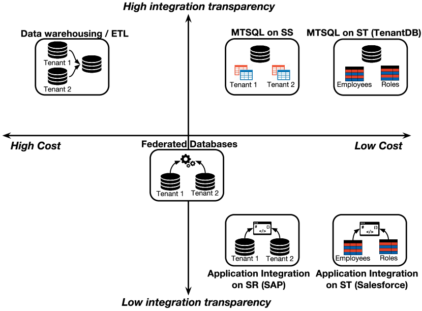
Figure 1: Cross-tenant query processing systems

Finally, there are the two schemes where tenants not only share a database, but also the table layout (schema). Either, as for example in Apache Phoenix [8], tenants still have their private tables, but these tables share the same (logical) schema (SS), or the data of different tenants is consolidated into shared tables (ST) which is hence the layout with the highest degree of physical and logical sharing. SS and ST layouts are not only used in DaaS, but also in Software-as-a-Service (SaaS) platforms, as for example in Salesforce [38] and FlexScheme [10, 11]. The main reason why these systems prefer ST over SS is cost [10]. Moreover, if the number of tenants exceeds the number of tables a database can hold ,which is typically a number in the range of ten thousands, SS becomes prohibitive. Conversely, ST databases can easily accommodate hundred thousands to even millions of tenants.

An important feature of multi-tenant databases, which we believe did not yet get the attention it deserves, is cross-tenant query processing. One compelling use case is health care where many providers and insurances use the same integrated SaaS application. If the providers would agree to query their joint datasets of (properly anonymized) patient data with scientific institutions, this could enable medical research to advance much faster because the data can be queried as soon as it gets in.

This paper looks into cross-tenant query processing within the scope of SS and ST databases, thereby optimizing a very specific sub-problem of data integration (DI). DI, in a broad sense, is about finding schema and data mappings between the original schemas of different data sources and a target schema specified by the client application [24, 21, 34]. As such, DI techniques are applicable to the entire spectrum of multi-tenant databases because even if tenants use different schemas or databases, these techniques can identify correlations and hence extract useful information. Our work embraces and builds on top of the latest DI work. More concretely, we optimize conversion functions similar to those used in DI by thoroughly analyzing and exploiting their algebraic properties. In addition, instead of translating data into a specific client format (and update periodically), we convert it to any required client format efficiently and just-in-time.

There are several existing approaches to cross-tenant query processing which are summarized in Figure 1: The first approach is data warehousing [25] where data is extracted from several data sources (tenant databases/tables), transformed into one common format and finally loaded into a new database where it can be queried by the client. This approach has high integration transparency in the sense that once the data is loaded, it is in the right format as required by the client and she can ask any query she wants. Moreover, as all data is in a single place, queries can be optimized. On the down-side of this approach, as argued by [13, 32, 9], are costs in terms of both, developing and maintaining such ETL pipelines and maintaining a separate copy of the data. Another disadvantage is data staleness in the presence of frequent updates.

Federated Databases [27, 23] reduce some of these costs by integrating data on demand, i.e. there is no copying. However, maintenance costs are still significant as for every new data source a new integrator/wrapper has to be developed. As data resides in different places (and different formats), queries can only be optimized to a very small extent (if at all), which is why the degree of integration transparency is considered sub-optimal. Finally, systems like SAP HANA [35] and Salesforce [38], which are mainly tailored towards single-tenant queries, offer some degree of cross-tenant query processing, but only through their application logic, which means that the set of queries that can be asked is limited.

The reason why none of these approaches tries to use SQL for cross-tenant query processing is that it is ambiguous. Consider, for instance the ST datbase in Figure 2, which we are going to use as a running example throught the paper: As soon as we want to query the joint dataset of tenants 0 and 1 and, for instance, join Employees with Roles, joining on role_id alone is not enough as this would also join Patrick with researcher and Ed with professor, which is clear nonsense. The obvious solution is to add the tenant-ID ttid to the join predicate. On the other hand, joining the Employees table with itself on E1.age = E2.age does not require ttid to be present in the join predicate because it actually makes sense to include results like (Alice, Ed) as they are indeed the same age. As ttid is an attribute invisible to the client, plain SQL has no way to distinguish the two cases, the one where ttid has to be included in the join and the one where it does not. Another challenge arises from the fact that different tenants might store their employees’ salaries in different currencies. If this is the case, computing the average salary across all tenants clearly involves some value conversions that should, ideally, happen without the client noticing or even worrying about.

This paper presents MTSQL as a solution to all these ambiguity problems. MTSQL extends SQL with additional semantics specifically-suited for cross-tenant query processing. It enables high integration transparency because any client, with any desired data format, can ask any query at any time. Moreover, as data resides in a single database (SS or ST), queries can be aggressively optimized with respect to both, standard SQL semantics and additional MTSQL semantics. As MTSQL adopts the single-database layout, it is also very cost-effective, especially if used on top of ST. Moreover, data conversion only happens as needed, which perfectly fits the cloud’s pay-as-you-go cost model. Specifically, the paper makes the following contributions:

• It defines the syntax and semantics of MTSQL, a query language that extends SQL with additional semantics suitable for cross-tenant query processing.

• It presents the design and implementation of MTBase, a database middleware that executes MTSQL on top of any ST database.

• It studies MTSQL-specific optimizations for query execution in MTBase.

• It extends the well-known TPC-H benchmark to run and evaluate MTSQL workloads.

• It evaluates the performance and the implementation correctness of MTBase with this benchmark.

The rest of this paper is organized as follows: Section 2 defines MTSQL while Section 3 gives an overview on MTBase. Section 4 discusses the MTSQL-specific optimizations, which are validated in Section 6 using the benchmark presented in Section 5. Section 7 shortly summarizes lines of related work while the paper is concluded in Section 8.

E_ttid	E_emp_id	E_name	E_role_id	E_reg_id	E_salary	E_age
0	0	Patrick	1	3	50K	30
0	1	John	0	3	70K	28
0	2	Alice	2	3	150K	46
1	0	Allan	1	2	80K	25
1	1	Nancy	2	4	200K	72
1	2	Ed	0	4	1M	46

Employees (tenant-specific),
E_salary of tenant 0 in USD, E_salary of tenant 1 in EUR

R_ttid	R_role_id	R_name
0	0	phD stud.
0	1	postdoc
0	2	professor
1	0	intern
1	1	researcher
1	2	executive

Roles (tenant-specific)

Re_reg_id	Re_name
0	AFRICA
1	ASIA
2	AUSTRALIA
3	EUROPE
4	N-AMERICA
5	S-AMERICA

Regions (global)

Figure 2: MTSQL database in Basic Layout (ST),
$ttid$s not visible to clients

E_emp_id	E_name	E_role_id	E_reg_id	E_salary	E_age
0	Patrick	1	3	50K	30
1	John	0	3	70K	28
2	Alice	2	3	150K	46

Employees_0 (private), E_salary in USD

E_emp_id	E_name	E_role_id	E_reg_id	E_salary	E_age
0	Allan	1	2	80K	25
1	Nancy	2	4	200K	72
2	Ed	0	4	1M	46

Employees_1 (private), E_salary in EUR

R_role_id	R_name
0	phD stud.
1	postdoc
2	professor

Roles_0 (private)

R_role_id	R_name
0	intern
1	researcher
2	executive

Roles_1 (private)

Re_reg_id	Re_name
0	AFRICA
1	ASIA
2	AUSTRALIA
3	EUROPE
4	N-AMERICA
5	S-AMERICA

Regions (global)

Figure 3: MTSQL database in Private Table Layout (SS)

2 MTSQL

In order to model the specific aspects of cross-tenant query processing in multi-tenant databases, we developed MTSQL, which will be described in this section. MTSQL extends SQL in two ways: First, it extends the SQL interface with two additional parameters, $C$ and $D$. $C$ is the tenant ID (or ttid for short) of the client who submits a statement and hence determines the format in which the result must be presented. The data set, $D$, is a set of ttids that refer to the tenants whose data the client wants to query. Secondly, MTSQL extends the syntax and semantics of SQL, as well as its Data Definition Language (DDL), Data Manipulation Language (DML) and Data Control Language (DCL, consists of GRANT and REVOKE statements).

As mentioned in the introduction, there are several ways how a multi-tenant database can be laid out: Figure 2 shows an example of the ST scheme, also referred to as basic layout in related work [10] where tenants’s data is consolidated using the same tables. Meanwhile, Figure 3 illustrated the SS scheme, also referred to as private table layout, where every tenant has her own set of tables. In that scheme, data ownership is defines as part of the table name while in ST, records are explicitly annotated with the ttid of their data owner, using an extra meta column in the table which is invisible to the client.

As these two approaches are semantically equivalent, the MTSQL semantics that we are about to define apply to both. In the case of the SS, applying a statement $s$ with respect to $D$ simply means to apply $s$ to the logical union of all private tables owned by a tenant in $D$. In SS, $s$ is applied to tables filtered according to $D$. In order to keep the presentation simple, the rest of this paper assumes an ST scheme, but sometimes defines semantics with respect to SS if that makes the presentation easier to understand.

2.1 MTSQL API

MTSQL needs a way to incorporate the additional parameters $C$ and $D$. As $C$ is the ttid of the tenant that issues a statement, we assume it is implicitly given by the SQL connection string. ttids are not only used for identification and access control, but also for data ownership (as shown in Figure 3). While this paper uses integers for simplicity reasons, ttids can have any data type, in particular they can also be database user names.

$D$ is defined using the MTSQL-specific SCOPE runtime parameter on the SQL connection. This parameter can be set in two different ways: Either, as shown in Listing 1, as simple scope with an IN list stating the set of ttids that should be queried, or as in Listing 2, as a sub-query with a FROM and a WHERE clause (complex scope). The semantics of the latter is that every tenant that owns at least one record in one of the tables mentioned in the FROM clause that satisfies the WHERE clause is part of $D$. The SCOPE variable defaults to $\{C\}$, which means that by default a client processes only her own data. Defining a simple scope with an empty IN list, on the other hand, makes $D$ include all the tenants present in the database.

Making $C$ and $D$ part of the connection allowed for a clear separation between the end users of MTSQL (for which ttids do not make much sense and hence remain invisible) and administrators/programmers that manage connections (and are aware of ttids).

⬇

SET SCOPE = "IN (1,3,42)";

Listing 1: Simple SCOPE expression using IN

⬇

SET SCOPE = "FROM Employees WHERE E_salary > 180K";

Listing 2: Complex SCOPE expression with sub-query

2.2 Data Definition Language

DDL statements are issued by a special role called the data modeller. In a multi-tenant application, this would be the SaaS provider (e.g. a Salesforce administrator) or the provider of a specific application. However, the data modeller can delegate this privilege to any tenant she trusts using a GRANT statement, as will be described in § 2.3.

There are two types of tables in MTSQL: tables that contain common knowledge shared by everybody (like Regions) and those that contain data of a specific tenant (i.e. Employees and Roles). More formally, we define the table generality of Regions as global and the one of all other tables as tenant-specific. In order to process queries across tenants, MTSQL needs a way to distinguish whether an attribute is comparable (can be directly compared against attribute values of other tenants), convertible (can be compared against attribute values of other tenants after applying a well-defined conversion function) or tenant-specific (it does semantically not make sense to compare against attribute values of other tenants). An overview of these types of attribute comparability, together with examples from Figure 2, is shown in Figure 2.

type	description	examples
comparable	can be directly compared to and aggregated with other values	E_region_id, E_age, Re_name, R_region_id, R_name
convertible	other values need to be converted to the format of the current tenant before comparison or aggregation	E_salary
tenant-specific	values of different tenants cannot be compared with each other	E_role_id, R.role_id

Table 2: Overview on attribute comparability in MTSQL

2.2.1 CREATE TABLE Statement

The MTSQL-specific keywords for creating (or altering) tables are GLOBAL, SPECIFIC, COMPARABLE and CONVERTIBLE. An example of how they can be used is shown in Listing 3. Note that SPECIFIC can be used for tables and attributes. Moreover, using these keywords is optional as we define that tables are global by default, attributes of tenant-specific tables default to tenant-specific and those of global tables to comparable.

⬇

1CREATE TABLE Employees SPECIFIC (

2 E_emp_id INTEGER NOT NULL SPECIFIC,

3 E_name VARCHAR(25) NOT NULL COMPARABLE,

4 E_role_id INTEGER NOT NULL SPECIFIC,

5 E_reg_id INTEGER NOT NULL COMPARABLE,

6 E_salary VARCHAR(17) NOT NULL CONVERTIBLE @currencyToUniversal @currencyFromUniversal,

7 E_age INTEGER NOT NULL COMPARABLE,

8 CONSTRAINT pk_emp PRIMARY KEY (E_emp_id),

9 CONSTRAINT fk_emp FOREIGN KEY (E_role_id) REFERENCES Roles (R_role_id)

10);

Listing 3: Exemplary MTSQL CREATE TABLE statement, MT-specific keywords marked in bold

2.2.2 Conversion Functions

Cross-tenant query processing requires the ability to execute comparison predicates on comparable and convertible attribute. While comparable attributes can be directly compared to each other, convertible attributes, as their name indicates, have to be converted first, using conversion functions. Each tenant has a pair of conversion functions for each attribute to translate from and to a well-defined universal format. More formally, a conversion function pair is defined as follows:

Definition 1

$(toUniversal:X\times T\rightarrow X,from$-$Universal:X\times T\rightarrow X)$ is a valid MTSQL conversion function pair for attribute $A$, where $T$ is the set of tenants in the database and $X$ is the domain of $A$, if and only if:

1. There exists a universal format for attribute $A$:
   $image(toUniversal(\cdot,t_{1}))=image(toUniversal(\cdot,t_{2}))$
   $=\ldots=image(toUniversal(\cdot,t_{|T|}))$

2. For every tenant $t\in T$, the partial functions $toUniversal(\cdot,t)$ and $fromUniversal(\cdot,t)$ are bijective functions.

3. $fromUniversal$ is the inverse of $toUniversal$: $\forall t\in T,\linebreak x\in X:fromUniversal(toUniversal(x,t),t)=x$

These three properties imply the following two corollaries that we are going to need later in this paper:

Corollary 1

$toUniversal$ and $fromUniversal$ are equality preserving: $\forall t\in T:toUniversal(x,t)=toUniversal(y,t)\Leftrightarrow x=y\Leftrightarrow fromUniversal(x,t)=fromUniversal(y,t)$

Corollary 2

Values from any tenant $t_{i}$ can be converted into the representation of any other tenant $t_{j}$ by first applying $toUniversal(\cdot,t_{i})$, followed by $fromUniversal(\cdot,t_{j})$ while equality is preserved:

$$\forall t_{i},t_{j}\in T:x=y\Leftrightarrow fromUniversal(toUniversal(x,t_{i}),t_{j})$$

$$= fromUniversal(toUniversal(y,t_{i}),t_{j})$$

The reason why we opted for a two-step conversion through universal format is that it allows each tenant $t_{i}$ to define her share of the conversion function pair, i.e. $toUniversal(\cdot,t_{i})$ and $from$-$Universal(\cdot,t_{i})$, individually without the need of a central authority. Moreover, this design greatly reduces the overall number of partial conversion functions as we need at most $2\cdot|T|$ partial function definitions, compared to $|T|^{2}$ functions in the case where we would define a direct conversion for every pair of tenants.

Listings 4 and 5 show an example of such a conversion function pair. These functions are used to convert phone numbers with different prefixes, like “+”, “00” or any other specific county exit code, and the universal format is a phone number without prefix. In this example, converting phone numbers simply means to lookup the tenant’s prefix and then either prepend or remove it, depending whether we convert from or to the universal format. Note that the exemplary code also contains the keyword IMMUTABLE to state that for a specific input the function always returns the same output, which is an important hint for the query optimizer. While this keyword is PostgreSQL-specific, some other vendors, but by far not all, offer a similar syntax.

⬇

38CREATE FUNCTION phoneToUniversal (VARCHAR(17), INTEGER) RETURNS VARCHAR(17)

39 AS ’SELECT SUBSTRING($1, CHAR_LENGTH(PT_prefix)+1) FROM Tenant, PhoneTransform WHERE T_tenant_key = $2 AND T_phone_prefix_key = PT_phone_prefix_key;’

40LANGUAGE SQL IMMUTABLE;

Listing 4: Converting a phone number to universal form (without prefix), PostgreSQL syntax

⬇

42CREATE FUNCTION phoneFromUniversal (VARCHAR(17), INTEGER) RETURNS VARCHAR(17)

43 AS ’SELECT CONCAT(PT_prefix, $1) FROM Tenant, PhoneTransform WHERE T_tenant_key = $2 AND T_phone_prefix_key = PT_phone_prefix_key;’

44LANGUAGE SQL IMMUTABLE;

Listing 5: Converting to a specific phone number format, PostgreSQL syntax

It is important to mention that the equality-preserving property as mentioned in Corollary 1 is a minimal requirement for conversion functions to make sense in terms of producing coherent query results among different clients. There are, however conversion functions that exhibit additional properties, for example:

• order-preserving with respect to tenant $t$:
  $x<y\Leftrightarrow toUniversal(x,t)<toUniversal(y,t)$

• homomorphic with respect to tenant $t$ and function $h$:
  $toUniversal(h(x_{1},x_{2},...),t)=$
  $h(toUniversal(x_{1},t),toUniversal(x_{2},t),...)$

We will call a conversion function pair fully-order-preserving if $toUniversal$ and $fromUniversal$ are order-preserving with respect to all tenants. Consequently, a conversion function pair can also be fully-h-preserving.

Listings 6 and 7 show an exemplary conversion function pair used to convert currencies (with USD as universal format). These functions are not only equality-preserving, but also fully-SUM-preserving: as the currency conversion is nothing but a multiplication with a constant factor from CurrencyTransform, it does not matter in which format we sum up individual values (as long as they all have that same format). As we will see, such special properties of conversion functions are another crucial ingredient for query optimization.

⬇

30CREATE FUNCTION currencyToUniversal (DECIMAL(15,2), INTEGER) RETURNS DECIMAL(15,2)

31 AS ’SELECT CT_to_universal*$1 FROM Tenant, CurrencyTransform WHERE T_tenant_key = $2 AND T_currency_key = CT_currency_key;’

32LANGUAGE SQL IMMUTABLE;

Listing 6: Converting a currency to universal form (USD), PostgreSQL syntax

⬇

34CREATE FUNCTION currencyFromUniversal (DECIMAL(15,2), INTEGER) RETURNS DECIMAL(15,2)

35 AS ’SELECT CT_from_universal*$1 FROM Tenant, CurrencyTransform WHERE T_tenant_key = $2 AND T_currency_key = CT_currency_key;’

36LANGUAGE SQL IMMUTABLE;

Listing 7: Converting from USD to a specific currency, PostgreSQL syntax

The conversion function examples shown in Listings 4 to 7 assume the existence of tables holding additional conversion information (CurrencyTransmform and PhoneTransform) as well as a table with references into these tables (named Tenants table). The way how a tenant can define her portion of the conversion functions is then simply to choose a specific currency and phone format as part of an initial setup procedure. However, this is only one possible implementation. MTSQL does not make any assumptions or restrictions on the implementation of conversion function pairs themselves, as long as they satisfy the properties given in Definition 1.

MTSQL is not the first work that talks about conversion functions. In fact, there is an entire line of work that deals with data integration and in particular with schema mapping techniques [24, 21, 10]. These works mention and take into account conversion functions, like for example a multiplication or a division by a constant. More complex conversion functions, including regular-expression-based substitutions and other arithmetic operations, can be found in Potter’s Wheel [34] where conversion is referred to as value translation. All these different conversion functions can potentially also be used in MTSQL which is, to the best of our knowledge, the first work that formally defines and categorizes conversion functions according to their properties.

2.2.3 Integrity Constraints

MTSQL allows for global integrity constraints that every tenant has to adhere to (with respect to the entirety of her data) as well as tenant-specific integrity constraints (that tenants can additionally impose on their own data). An example of a global referential integrity constraint is shown in the end of Listing 3. This constraint means that for every tenant, for each entry of E_role_id, a corresponding entry R_role_id has to exist in Roles and must be owned by that same tenant. Consider for example employee John withR_role_id 0. The constraint implies that their must be a role 0 owned by tenant 0, which in that case is PhD student. If the constraint were only tenant-specific for tenant 1, John would not link to roles and E_role_id 0 would just be an arbitrary numerical value. In order to differentiate global from tenant-specific constraints, the scope is used.

2.2.4 Other DDL Statements

CREATE VIEW statements look the same as in plain SQL. As for the other DDL statements, anyone with the necessary privilege can define global views on global and tenant-specific tables. Tenants are allowed to create their own, tenant-specific views (using the default scope). The selected data has to be presented in universal format if it is a global view and in the tenant-specific format otherwise. DROP VIEW, DROP TABLE and ALTER TABLE work the same way as in plain SQL.

2.3 Data Control Language

Let us have a look at the MTSQL GRANT statement:

⬇

GRANT <privileges> ON <database|table> TO <ttid>;

Listing 8: MTSQL GRANT syntax

As in plain SQL, this grants some set of access privileges (READ, INSERT, UPDATE and/or DELETE) to the tenant identified by $ttid$. In the context of MTSQL, however, this means that the privileges are granted with respect to $C$. Consider the following statement:

⬇

GRANT READ ON Employees TO 42;

Listing 9: Example of an MTSQL GRANT statement

In the private table layout, if $C$ is 0, then this would grant tenant 42 read access to Employees_0, but if $C$ is 1, tenant 42 would get read access to Employees_1 instead. If a grant statement grants to $ALL$, then the grant semantics also depend on $D$, more concretely if $D=\{7,11,15\}$ the privileges would be granted to tenants 7, 11 and 15.

By default, a new tenant that joins an MTSQL system is granted the following privileges: READ access to global tables, READ, INSERT, UPDATE, DELETE, GRANT and REVOKE on his own instances of tenant-specific tables. In our example, this means that a new tenant 111 can read and modify data in Employees_111 and Roles_111. Next, a tenant can start asking around to get privileges on other tenants’ tables or also on global tables. The REVOKE statement, as in plain SQL, simply revokes privileges that were granted with GRANT.

2.4 Query Language

Just as in FlexScheme [10, 11], queries themselves are written in plain SQL and have to be filtered according to $D$. Whereas in FlexScheme $D$ always equals $\{C\}$ (a tenant can only query her own data), MTSQL allows cross-tenant query processing, which means that the data set can include other tenants than $C$ and can in particular be bigger than one. As mentioned in the introduction, this creates some new challenges that have to be handled with special care.

Figure 4: MTBase architecture

2.4.1 Client Presentation

As soon as tenants can query other tenants’ data, the MTSQL engine has to be make sure to deliver results in the proper format. For instance, looking again at Figure 2, if tenant 0 queries the average salary of all employees of tenant 1, then this should be presented in USD because tenant 0 stores her own data in USD and expects other data to be in USD as well. Consequently, if tenant 1 would ask that same query, the result would be returned as is, namely in EUR.

2.4.2 Comparisons

Consider a join of Roles and Employees on reg_id. As long as the dataset size is only one, such a join query has the same semantics as in plain SQL (or FlexScheme). However, as soon as tenant 1, for instance, asks this query with $D=\{0,1\}$, the join has to take the ttids into account. The reason for this is that reg_id is a tenant-specific attribute and should hence only be joined within the same tenant in order to prevent semantically wrong results like John being an intern (although tenant 0 does not have such a role) or Nancy being a professor (despite the fact that tenant 1 only has roles intern, researcher and executive).

Comparison or join predicates containing comparable and convertible attributes, on the other hand, just have to make sure that all data is brought into universal format before being compared. For instance, if tenant 0 wants to get the list of all employees (of both tenants) that earn more than 100K USD, all employee salaries have to be converted to USD before executing the comparison.

Finally, MTSQL does not allow to compare tenant-specific with other attributes. For instance, we see no way how it could make sense to compare E_role_id to something like E_age or E_salary.

2.5 Data Manipulation Language

MTSQL DML works the same way as in FlexScheme [10, 11] if $D=\{C\}$. Otherwise, if $D\neq\{C\}$, the semantics of a DML statement are defined such that it is applied to each tenant in $D$ separately. Constants, WHERE clauses and sub-queries are interpreted with respect to $C$, exactly the same way as for queries (c.f. § 2.4). This implies that executing UPDATE or INSERT statements might involve value conversion to the proper tenant format(s).

3 MTBase

Based on the concepts described in the previous section, we implemented MTBase, an open-source MTSQL engine [3]. As shown in Figure 4, the basic building block of MTBase is an MTSQL-to-SQL translation middleware sitting between a traditional DBMS and the client. In fact, as it communicates to the DBMS (and to the client) by the means of pure SQL, MTBase works in conjunction with any off-the-shelve DBMS. For performance reasons, the proxy maintains a cache of MT-specific meta data, which is persisted in the DBMS along with the actual user data. Conversion functions are implemented as UDFs that might involve additional meta tables, both of which are also persisted in the DBMS. MTBase implements the basic data layout, which means that data ownership is implemented as an additional (meta) $ttid$ column in each tenant-specific table as illustrated in Figure 2). There are some dedicated meta tables: Tenant stores each tenant’s privileges and conversion information and Schema stores information about table and attribute comparability. Additional meta tables can (but do not have to) be used to implement conversion function pairs, as for example CurrencyTransform and PhoneTransform shown in Listings 4 to 7.

While the rewrite module was implemented in Haskell and compiled with GHC [5], the connection handling and the meta data cache maintenance was written in Python (and run with the Python2 interpreter) [1]. Haskell is handy because we can make full use of pattern matching and additive data types to implement the rewrite algorithm in a quick and easy-to-verify way, but any other functional language, like e.g. Scala [2], would also do the job. Likewise, there is nothing fundamental in using Python, any other framework that has a good-enough abstraction of SQL connections, e.g. JDBC [6], could be used.

Upon opening a connection at the middleware, the client’s $ttid$, $C$, is derived from the connection string and used throughout the entire lifetime of that connection. Whenever a client sends a MTSQL statement $s$, first if the current scope is complex, a SQL query $q_{s}$ is derived from this scope and evaluated at the DBMS in order to determine the relevant dataset $D$. After that, $D$ is compared against privileges of $C$ in the Tenant table and $ttid$s in $D$ without the corresponding privilege are pruned, resulting in $D^{\prime}$. Next, $C$, $D^{\prime}$ and $s$ are input into the rewrite algorithm which produces a rewritten SQL statement $s^{\prime}$ which is then sent to the DBMS before relaying the result back to the client. Note that in order to guarantee correctness in the presence of updates, $q_{s}$ and $s^{\prime}$ have to be executed within the same transaction and with a consistency level at least repeatable-read [12] (even if the client does not impose any transactional guarantees). If $s$ is a DDL statement, the middleware also updates the MT-Specific meta information in the DBMS and the cache.

The rest of this section explains the MTSQL-to-SQL rewrite algorithm in its canonical form and proves its correctness with respect to § 2.4, while Section 4 shows how to optimize the rewritten queries such that they can be run on the DBMS with reasonable performance.

3.1 Canonical Query Rewrite Algorithm

Our proposed canonical MTSQL-to-SQL rewrite algorithm works top-down, starting with the outer-most SQL query and recursively rewriting sub-queries as they come along. For each sub-query, the SQL clauses are rewritten one-by-one. The algorithm makes sure that for each sub-query the following invariant holds: the result of the sub-query is filtered according to $D^{\prime}$ and presented in the format required by $C$.

The pseudo code of the general rewrite algorithm for rewriting a (sub-)query is shown in Algorithm 1. Note that FROM, GROUP BY, ORDER BY and HAVING clause can be rewritten without any additional context while SELECT and WHERE need the whole query as an input because they might need to check the FROM for additional information, for instance they must know to which original tables certain attributes belong.

1:Input:   $C$: $ttid$, $D$: set of $ttid$s, $Q$: MTSQL query

2:Output: SQL query

3:function RewriteQuery($C,D,Q$)

4:     $new$-$select\leftarrow$ rewriteSelect($C$,$D$,$Q$)

5:     $new$-$from\leftarrow$ rewriteFrom($C$,$D$,$Q$.from())

6:     $new$-$where\leftarrow$ rewriteWhere($C$,$D$,$Q$)

7:     $new$-$group$-$by\leftarrow$ rewriteGroupBy($C$,$D$,$Q$.groupBy())

8:     $new$-$order$-$by\leftarrow$ rewriteOrderBy($C$,$D$,$Q$.orderBy())

9:     $new$-$having\leftarrow$ rewriteHaving($C$,$D$,$Q$.having())

10:     return new Query ($new$-$select$, $new$-$from$, $new$-$where$, $new$-$group$-$by$, $new$-$order$-$by$, $new$-$having$)

Algorithm 1 Canonical Query Rewrite Algorithm

In the following, we will look at the rewrite functions for the different SQL clauses. Because of space constraints, we only provide the high-level ideas and illustrate them with suitable minimal examples. However, we strongly encourage the interested reader to check-out the Haskell code [4] which in fact almost reads like a mathematical definition of the rewrite algorithm.

⬇

1-- Rewriting a simple select expression:

2SELECT E_salary FROM Employees; -->

3SELECT currencyFromUniversal(currencyToUniversal(E_salary, ttid), C) as salary FROM Employees;

4-- Rewriting an aggregated select expression

5SELECT AVG(E_salary) as avg_sal FROM Employees; -->

6SELECT AVG(currencyFromUniversal(currencyToUniversal(E_salary, ttid), C)) as avg_sal FROM Employees;

7-- Rewriting star expression, hiding irrelevant info

8SELECT * FROM Employees; -->

9SELECT E_name, E_reg_id, E_salary, E_age FROM Employees;

Listing 10: Examples for Rewriting SELECT clause

SELECT    The rewritten SELECT clause has to present every attribute $a$ in $C$’s format, which, if $a$ is convertible, is achieved by two calls to the conversion function pair of $a$ as can be seen in the examples of Listing 10 where - -> simply denotes rewriting. If $a$ is part of compound expression (as in line 6), it has to be converted before the functions (in that case $AVG$) are applied. Note that in order to make a potential super-query work correctly, we also rename the result of the conversion, either by the new name that it got anyway (as in line 6) or by the name that it had before (as in line 3). Rewriting a star expression (line 9) in the uppermost query also needs special attention, in order not to provide the client with confusing information, like $ttids$ which should stay invisible.

⬇

1-- Comparison with a constant:

2.. FROM Employees WHERE E_salary > 50K -->

3.. WHERE currencyFromUniversal(currencyToUniversal(E_salary,ttid),C) > 50K) ..

4-- General comparison:

5.. FROM Employees E1, Employees E2 WHERE E1.E_salary > E2.E_salary -->

6.. WHERE currencyFromUniversal(currencyToUniversal(E1.E_salary,E1.ttid),C) > currencyFromUniversal(currencyToUniversal(E1.E_salary,E1.ttid),C) ..

7-- Extend with predicate on ttid

8.. FROM Employees, Roles WHERE E_role_id = R_role_id -->

9.. FROM Employees, Roles WHERE E_role_id = R_role_id AND Employees.ttid = Roles.ttid ..

10-- Adding D-filters for D’ = {3,7}

11.. FROM Employees E, Roles R .. -->

12.. WHERE E.ttid IN (3,7) AND R.ttid IN (3,7) ..

Listing 11: Examples for Rewriting WHERE clause

WHERE    There are essentially three steps that the algorithm has to perform in order to create a correctly rewritten WHERE clause (as shown in Listing 11). First, conversion functions have to be added to each convertible attribute in each predicate in order make sure that comparisons are executed in the correct (client) format (lines 2 to 6). This happens the same way as for a SELECT clause. Notably, all constants are always in $C$’s format because it is $C$ who asks the query. Second, for every predicate involving two or more tenant-specific attributes, additional predicates on $ttid$ have to be added (line 9), unless if the attributes are part of the same table, which means they are owned by the same tenant anyway. Predicates that contain tenant-specific together with other attributes cause the entire query to be rejected as was required in § 2.4.2. Last, but not least, for every base table in the FROM clause, a so-called D-filter has to be added to the WHERE clause (line 12). This filter makes sure that only the relevant data (data that is owned by a tenant in $D^{\prime}$) gets processed.

FROM    All tables referred by the FROM clause are either base tables or temporary tables derived from a sub-query. Rewriting the FROM clause simply means to call the rewrite algorithm on each referenced sub-query as shown in Algorithm 2. A FROM table might also contain a JOIN of two tables (sub-queries). In that case, the two sub-queries are rewritten and then the join predicate is rewritten in the exact same way like any WHERE.

Notably, this algorithm preserves the desired invariant for (sub-) queries: the result of each sub-query is in client format and filtered according to $D^{\prime}$, and, due to the rewrite of the SELECT and the WHERE clause of the current query, base tables, as well as joins, are also presented in client format and filtered by $D$. We conclude that the result of the current query therefore also preserves the invariant.

1:Input:   $C$: $ttid$, $D$: set of $ttid$s,

2:          $FromClause$: MTSQL FROM clause

3:Output: SQL FROM clause

4:function RewriteFrom($C,D,FromClause$)

5:     $res\leftarrow$ extractBaseTables $(FromClause)$

6:     for all $q\in$ extractSubQueries $(FromClause)$ do

7:         $res\leftarrow res\cup\{$ rewriteQuery $(C,D,q)\}$      

8:     for all $(q_{1},q_{2},cond)\in$ extractJoins $(FromClause)$ do

9:         $q_{1}^{\prime}\leftarrow$ rewriteQuery $(C,D,q_{1})$

10:         $q_{2}^{\prime}\leftarrow$ rewriteQuery $(C,D,q_{2})$

11:         $cond^{\prime}\leftarrow$ rewriteWhere $(C,D,cond)$

12:         $res\leftarrow res\cup\{$ createJoin $(q_{1}^{\prime},q_{2}^{\prime},cond^{\prime}))\}$      return $res$

Algorithm 2 Rewrite Algorithm for FROM clause

GROUP-BY, ORDER-BY and HAVING    HAVING andGROUP-BY clauses are basically rewritten the same way like the expressions in the SELECT clause. Some DBMSs might throw a warning stating that grouping by a comparable attribute $a$ is ambiguous because the way we rewrite $a$ in the WHERE clause and rename it back to $a$, we could actually group by the original or by the converted attribute $a$. However, the SQL standard clearly says that in such a case, the result should be grouped by the outer-more expression, which is exactly what we need. ORDER-BY clauses need not be rewritten at all.

SET SCOPE    Simple scopes do not have to be rewritten at all. The FROM and WHERE clause of a complex scope are rewritten the same way as in a sub-query. In order to make it a valid SQL query, the rewrite algorithm adds a SELECT clause that projects on the respective $ttid$s as shown in Listing 12.

⬇

1SET SCOPE = "FROM Employees WHERE E_salary > 180K"; -->

2SELECT ttid FROM Employees WHERE currencyFromUniversal(currencyToUniversal(E_salary,ttid),C) > 180K;

Listing 12: Rewriting a complex SCOPE expression

3.2 Algorithm Correctness

Proof 3.1.

We prove the correctness of the canonical rewrite algorithm with respect to § 2.4 by induction over the composable structure of SQL queries and by showing that the desired invariant (the result of each sub-query is filtered according to $D^{\prime}$ and presented in the format required by $C$) holds: First, as a base, we state that adding the D-filters in the WHERE clause and transforming the SELECT clause to client format for every base table in each lowest-level sub-query ensures that the invariant holds. Next, as an induction step, we state that the way how we rewrite the FROM clause, as it was described earlier, preserves that property. The top-most SQL query is nothing but a composition of sub-queries (and base tables) for which the invariant holds. This means that the invariant holds for the entire query, which is hence guaranteed to deliver the correct result.

3.3 Rewriting DDL and DML Statements

Rewriting DDL and DML statements is very similar to rewriting queries, in fact, predicates are rewritten in exactly the same way. The remaining questions are how to rewrite tenant-specific referential integrity constraints (using check constraints) and how to apply DML statements to a dataset $D\neq\{C\}$ (by executing the proper value transformations separately for each client). While the semantics and the intuition how to implement them should be clear, we refer to Appendix A for further examples and explanations.

4 Optimizations

As we have seen, there is a canonical rewrite algorithm that correctly rewrites MTSQL to SQL. However, we will show in Section 6 that the rewritten queries often execute very slowly on the underlying DBMS. The main reason for this is that the pure rewritten queries call two conversion functions on every transformable attribute of every record that is processed, which is extremely expensive. Luckily, the execution costs can be reduced dramatically when applying the optimization passes that we describe in this section. As we assume the underlying DBMS to optimize query execution anyway, we focus on optimizations that a DBMS query optimizer cannot do (because it needs MT-specific context) or does not do (because an optimization is not frequent enough outside the context of MTBase). We differentiate between semantic optimizations, which are always applied because they never make a query slower and cost-based optimizations which are only applied if the predicted costs are smaller than in the original query.

⬇

1-- dropping D-filter if D is the empty scope:

2SELECT E_age FROM Employees WHERE E_ttid IN (1,2); -->

3SELECT E_age FROM Employees;

4-- dropping ttid from join predicate if |D| = 1:

5SELECT E_age, R_name FROM Employees, Roles WHERE E_role_id = R_role_id AND E_ttid = R_ttid AND E_ttid IN (2) AND R_ttid IN (2); -->

6SELECT E_age, R_name FROM Employees, Roles WHERE E_role_id = R_role_id AND E_ttid IN (2) AND R_ttid IN (2);

7-- dropping conversion functions if D = {C}:

8SELECT currencyFromUniversal(currencyToUniversal(E_salary, E_ttid),0) AS E_salary FROM Employees; -->

9SELECT E_salary FROM Employees;

Listing 13: Examples for trivial semantic optimizations

4.1 Trivial Semantic Optimizations

There are a couple of special cases for $C$ and $D$ that allow to save conversion function calls, join predicates and/or D-filters. First, if $D$ includes all tenants, that means that we want to query all data and hence D-filters are no longer required as shown in line 3 of Listing13. Second, as shown in line 6, if $|D|=1$, we know that all data is from the same tenant, which means that including ttid in the join predicate is no longer necessary. Last, if we know that a client queries her own data, i.e. $D=\{C\}$ corresponds to the default scope, we know that even convertible attributes are already in the correct format and can hence remove the conversion function calls (line 9).

4.2 Other Semantic Optimizations

There are a couple of other semantic optimizations that can be applied to rewritten queries. While client presentation push-up and conversion push-up minimize the number of conversions by delaying conversion to the latest possible moment, aggregation distribution takes into account specific properties of conversion functions (as mentioned in § 2.2.2). If conversion functions are UDFs written in SQL it is also possible to inline them. This typically gives queries an additional speed up.

4.2.1 Client Presentation and Conversion Push-Up

As conversion function pairs are equality-preserving, it is possible in some cases to defer conversions to later, for example to the outermost query in the case of nested queries. While client presentation push-up converts everything to universal format and defers conversion to client format to the outermost SELECT clause, conversion push-up pushes this idea even more by also delaying the conversion to universal format as much as possible. Both optimizations are beneficial if the delaying of conversions allows the query execution engine to evaluate other (less expensive) predicates first. This means that, once the data has to be converted, it is already more filtered and therefore the overall number of (expensive) conversion function calls becomes smaller (or, in the worst case, stays the same). Naturally, if we delay conversion, this also means that we have to propagate the necessary ttids to the outer-more queries and keep track of the current data format.

⬇

1-- before optimization

2SELECT Dom.name1, Dom.sal1 as sal, COUNT(*) as cnt FROM (

3 SELECT E1.name as name1, currencyFromUniversal(currencyToUniversal(E1.E_salary, E1.E_ttid), C) as sal1

4 FROM Employees E1, Employees E2

5 WHERE currencyFromUniversal(currencyToUniversal(E1.E_salary, E1.E_ttid), C) >

6 currencyFromUniversal(currencyToUniversal(E2.E_salary, E2.E_ttid), C)

7) as Dom GROUP BY Dom.name1, sal, cnt ORDER BY cnt;

8-- after optmimization

9SELECT Dom.name1, currencyFromUniversal(Dom.sal1, C) as sal, COUNT(*) as cnt FROM (

10 SELECT E1.name as name1, currencyToUniversal(E1.E_salary, E1.E_ttid) as sal1

11 FROM Employees E1, Employees E2

12 WHERE currencyToUniversal(E1.E_salary, E1.E_ttid) > currencyToUniversal(E2.E_salary, E2.E_ttid)

13) as Dom GROUP BY Dom.name1, sal, cnt ORDER BY cnt;

Listing 14: Example for client presentation push-up

Listing 14 shows a query that ranks employees according to the fact how many salaries of other employees their own salary dominates. With client presentation push-up, salaries are compared in universal instead of client format, which is correct because of the equality-preserving property (c.f. Corollary 1) and saves half of the function calls in the sub-query.

Conversion push-up, as shown in Listing 15, reduces the number of function calls dramatically: First, as it only converts salaries in the end, salaries of employees aged less than 45 do not have to be considered at all. Second, the WHERE clause converts the constant (100K) instead of the attribute (E_salary). As the outcome of conversion functions is immutable (c.f. § 2.2.2) and $C$ is also constant, the conversion functions have to be called only once per tenant and are then cached by the DBMS for the rest of the query execution, which becomes much faster as we will see in Section 6.

⬇

1-- before optimization

2SELECT AVG(X.sal) FROM (

3 SELECT currencyFromUniversal(currencyToUniversal(E_salary, E_ttid), C) as sal

4 FROM Employees WHERE E_age >= 45 AND

5 currencyFromUniversal(currencyToUniversal(E_salary, E_ttid), C) > 100K) as X;

6-- after optimization

7SELECT AVG(currencyFromUniversal(currencyToUniversal(X.sal, X.sal_ttid),C)) FROM (

8 SELECT E_salary as sal, E_ttid as sal_ttid

9 FROM Employees WHERE E_age >= 45 AND

10 E_salary > currencyFromUniversal(currencyToUniversal(100K, E_ttid), C) as X);

Listing 15: Example for conversion push-up

4.2.2 Aggregation Distribution

Many analytical queries contain aggregation functions, some of which aggregate on convertible attributes. The idea of aggregation distribution is to aggregate in two steps: First, aggregate per tenant in that specific tenant format (requires no conversion) and second, convert intermediary results to universal (one conversion per tenant), aggregate those and convert the final result to client format (one additional conversion). This simple idea reduces the number of conversion function calls for $N$ records and $T$ different data owners of these records from $(2N)$ to $(T+1)$. This is significant because $T$ is typically much smaller than $N$ (and cannot be greater).

Compared to pure conversion push-up, which works for any conversion function pair, the applicability of aggregation distribution depends on further algebraic properties of these functions. Gray et al. [22] categorize numerical aggregation functions into three categories with regard to their ability to distribute: distributive functions, like COUNT, SUM, MIN and MAX distribute with functions $F$ (for partial) and $G$ (for total aggregation). For COUNT for instance, $F$ is COUNT and $G$ is SUM as the total count is the sum of all partial counts. There are also algebraic aggregation functions, e.g. AVG, where the partial results are not scalar values, but tuples. In the case of AVG, this would be the pairs of a partial sums and partial counts because the total average can be computed from the sum of all sums, divided by the sum of all counts. Finally, holistic aggregation functions cannot be distributed at all.

	$to(x)=c\cdot x$	$to(x)=a\cdot x+b$	to = order-
preserving	to = equality- preserving
COUNT	✓	✓	✓	✓
MIN	✓	✓	✓	✕
MAX	✓	✓	✓	✕
SUM	✓	✓	✕	✕
AVG	✓	✓	✕	✕
Holistic	✕	✕	✕	✕

Table 3: Distributability of different aggregation functions over different categories of conversion functions

We would like to extend the notion of Gray et al. [22] and define the distributability of an aggregation function $a$ with respect to a conversion function pair $(from,to)$. Table 3 shows some examples for different aggregation and conversion functions. First of all, we want to state that, as all conversion functions have scalar values as input and output, they are always fully-COUNT-preserving, which means that COUNT can be distributed over all sorts of conversion functions. Next, we observe that all order-preserving functions preserve the minimum and the maximum of a given set of numbers, which is why MIN and MAX distribute over the first three categories of conversion functions displayed in Table 3. We further notice that if $to$ (and consequently also $from$) is a multiplication with a constant (first column of Table 3), $to$ is fully- MIN-, fully-MAX- and fully-SUM-preserving, which is why these aggregation functions distribute. As SUM and COUNT distribute, AVG, an algebraic function, distributes as well.

Finally looking at the second column of Table 3, we see that even linear functions are SUM- and AVG-preserving. To see why, we can think about computing the average over all tenants as a weighted average of partial (per-tenant) averages for AVG and multiply these partial averages with the partial counts to reconstruct the total sum. This method is further explained and proven in Appendix B.

We conclude this subsection by observing that the conversion function pair for phone format (c.f. Listings 4 and 5) is not even order-preserving and does therefore not distribute while the pair for currency format (c.f. Listings 67) distributes over all standard SQL aggregation functions. An example of how this can be used is shown in Listing 16.

⬇

1-- before optimization

2SELECT SUM(currencyFromUniversal(currencyToUniversal(E_salary, E_ttid), C)) as sum_sal FROM Employees

3-- after optimization

4SELECT currencyFromUniversal(SUM(t.E_partial_salary), C) as sum_sal FROM (SELECT currencyToUniversal(SUM(E_salary), E_ttid) as E_partial_salary FROM Employees GROUP BY E_ttid) as t;

Listing 16: Example for conversion function distribution

4.2.3 Function Inlining

As explained in § 2.2.2, there are several ways how to define conversion functions. However, if they are defined as a SQL statement (potentially including lookups into meta tables), they can be directly inlined into the rewritten query in order to save calls to UDFs. Function inlining typically also enables the query optimizer of the underlying DBMS to optimize much more aggressively. In WHERE clauses, conversion functions could simply be inlined as sub-queries, which, however often results in sub-optimal performance as calling a sub-query on each conversion is not much cheaper than calling the corresponding UDF. For SELECT clauses, the SQL standard does anyway not allow to inline as a sub-query as this can result in attributes not being contained neither in an aggregate function nor in the GROUP BY clause, which is why most commercial DBMS reject such queries (while PostgreSQL, for instance executes them anyway). This is why the proper way to inline functions is by using a join as shown in Listing 17. Our results in Section 6 suggest that function inlining, though producing complex-looking SQL queries, results in very good query execution performance.

⬇

1-- before optimization

2SELECT currencyFromUniversal(currencyToUniversal(E_salary, E_ttid), C)) as E_salary FROM Employees

3-- after optimization

4SELECT (C1.CT_from_universal * C2.CT_to_universal * E_salary) as E_salary

5FROM Employees, Tenant T1, Tenant T2, CurrencyTransform1, CurrencyTransform2

6WHERE T1.T_tenant_key = C AND T1.T_currency_key = CurrencyTransform1.CT_currency_key AND

7T2.T_tenant_key = E_ttid AND T2.T_currency_key = CurrencyTransform2.CT_currency_key

Listing 17: Example for function inlining

5 MT-H Benchmark

As MTSQL is a novel language, their exists no benchmark to evaluate the performance on an engine that implements it, like for instance MTBase. So far, there exists no standard benchmark for cross-tenant query processing, only for data integration [36] which does not assume the data to be in shared tables. Transactions in MTBase are not much different from standard transactions. Analytical queries, however, typically involve a lot of conversions and therefore thousands of (potentially expensive) calls to UDFS. Thus, the ability to study the usefulness of different optimizations passes on different analytical queries was a primary design goal, which is why we decided to extend the well-known TPC-H database benchmark [37]. Our new benchmark, which we call MT-H, extends TPC-H in the following way:

• Each tenant represents a different company. The number of tenants $T$ is a parameter of the benchmark. ttids range from $1$ to $T$.

• We consider Nation, Region, Supplier, Part, andPartsupp common, publicly available knowledge. They are therefore global tables and need no modification.

• We consider Customer, Orders and Lineitem tenant-specific. While the latter two are quite obviously tenant-specific (each company processes their own orders and line items), customers might actually do business with several companies. However, as customer information might be sensitive and the format of this information might differ from tenant to tenant, it makes sense to have specific customers per tenant.

• All primary keys and foreign keys relating to tenant-specific tables (C_custkey, O_orderkey, O_custkey,L_orderkey) are tenant-specific. If not mentioned otherwise, the attributes in Customer, Orders andLineitem are comparable.

• We consider two domains for convertible attributes and corresponding functions: currency and phone format. currency refers to monetary values, i.e. C_acctbal,O_totalprice and L_extendedprice and uses the conversion functions from Listings 6 and 7. phone format is used in C_phone with the conversion function pair of Listings 4 and 5. We modified the data generator of TPC-H (dbgen) to take the specific currency and phone formats into account. Each tenant is assigned a random currency and phone format, except for tenant 1 who gets the universal format for both.

• The TPC-H scaling factor $sf$ also applies to our benchmark and dictates the overall size of the tables. After creating all records with dbgen, each record in Customer, Orders and Lineitem is assigned to a tenant in a way that foreign-key constraints are preserved (e.g. orders of a specific tenant link to a customer of that same tenant). There are two ways how this assignment happens, either uniform (each tenant gets the same amount of records) or zipfian (tenant 1 gets the biggest share and tenant $T$ the smallest). This tenant share distribution $\rho$ is another parameter of the benchmark.

• We use the same 22 queries and query parameters as TPC-H. Additionally, for each query run, we have to define the client $C$ who runs the queries as well as the dataset $D$ she wants to query.

• For query validation, we simply set $C=1$ and $D=\{1,2,$ $\ldots,T\}.$ That way, we make sure to process all data and that the result is presented in universal format and can therefore be compared to expected query results of the standard TPC-H. An exception are queries that contain joins on O_custkey = C_custkey. In MT-H, we make sure that each order links to a customer from the same tenant, thus the mapping between orders and customers is no longer the same as in TPC-H (where an order can potentially link to any customer). For such queries, we define the result from the canonical rewrite algorithm (without optimizations) to be the gold standard to validate against.

6 Experiments and Results

This section presents the evaluation of MTBase using the MT-H benchmark. We first evaluated the benefits of different optimization steps from Section 4 and found that the combination of all of these steps brings the biggest benefit. Second, we analyzed how MTBase scales with an increasing number of tenants. With all optimizations applied and for a dataset of 100 GB on a single machine, MTBase scales up to thousands of tenants with very little overhead. We also validated result correctness as explained in Section 5 and can report only positive results.

6.1 Setup

In our experiments, we used the following two setups: The first setup is a PostgreSQL 9.6 Beta installation, running on Debian Linux 4.1.12 on a 4x16 Core AMD Opteron 6174 processor with 256 GB of main memory. The second installation runs a commercial database (which we will call System C) on a commercial operating system and on the same processor with 512 GB of main memory. Although both machines have enough secondary storage capacity available, we decided to configure both database management systems to use in-memory backed files in order to achieve the best performance possible. Moreover, we configured the systems to use all available threads, which enabled intra-query parallelism.

Level	Q01	Q02	Q03	Q04	Q05	Q06	Q07	Q08	Q09	Q10	Q11	Q12	Q13	Q14	Q15	Q16	Q17	Q18	Q19	Q20	Q21	Q22
tpch-0.1G	2.6	0.11	0.27	0.35	0.15	0.29	0.18	0.14	0.59	0.36	0.081	0.37	0.26	0.27	0.77	0.12	0.081	0.89	0.12	0.13	0.57	0.081
canonical	84	1.0	0.55	0.65	0.32	1.0	0.29	0.36	4.9	0.91	0.37	0.55	0.63	0.98	3.1	1.2	0.49	1.7	0.3	2.8	0.66	2.0
o1	2.7	1.0	0.43	0.61	0.22	0.43	0.23	0.56	3.8	0.76	0.37	0.55	0.92	0.56	0.91	1.2	0.48	1.6	0.3	2.8	0.66	0.085
o2	2.7	1.0	0.42	0.61	0.22	0.43	0.22	0.57	3.9	0.76	0.38	0.55	0.89	0.56	0.96	1.2	0.5	1.7	0.3	2.8	0.67	0.085
o3	2.7	1.0	0.43	0.61	0.22	0.43	0.23	0.56	3.9	0.76	0.37	0.55	0.92	0.56	0.91	1.2	0.48	1.6	0.3	2.8	0.66	0.085
o4	2.7	1.0	0.43	0.62	0.22	0.43	0.23	0.61	4.1	0.78	0.39	0.56	0.9	0.57	1.0	1.2	0.51	1.7	0.31	3.1	0.67	0.085
inl-only	2.7	1.0	0.42	0.65	0.22	0.43	0.22	0.57	3.8	0.76	0.37	0.55	0.92	0.56	0.92	1.2	0.48	1.6	0.3	2.8	0.66	0.085

Table 4: Response times [sec] of 22 TPC-H queries for MTBase-on-PostgreSQL with, $sf=1$, $T=10$, $\rho=$ uniform, $C=1$,
$D=\{1\}$, for different levels of optimizations, versus TPC-H with $sf=0.1$

Level	Q01	Q02	Q03	Q04	Q05	Q06	Q07	Q08	Q09	Q10	Q11	Q12	Q13	Q14	Q15	Q16	Q17	Q18	Q19	Q20	Q21	Q22
tpch-0.1G	2.6	0.11	0.27	0.35	0.15	0.29	0.18	0.14	0.59	0.36	0.081	0.37	0.26	0.27	0.77	0.12	0.081	0.89	0.12	0.13	0.57	0.081
canonical	87	1.0	0.5	0.6	0.28	1.0	0.26	0.37	4.9	0.89	0.37	0.56	0.65	1.0	3.2	1.2	0.49	1.6	0.31	2.8	0.66	2.0
o1	87	1.0	0.5	0.69	0.33	1.0	0.27	0.38	5.2	0.9	0.39	0.56	0.92	1.0	3.1	1.2	0.51	1.6	0.32	3.1	0.68	2.0
o2	87	1.0	0.5	0.61	0.28	1.0	0.27	0.38	5.2	0.9	0.39	0.57	0.91	1.0	3.1	1.2	0.51	1.6	0.32	3.1	0.67	1.3
o3	32	1.0	0.45	0.63	0.28	0.44	0.24	0.37	4.3	0.83	0.38	0.56	0.91	1.1	1.9	1.3	0.51	1.6	0.32	3.1	0.67	1.3
o4	14	1.0	0.48	0.62	0.22	0.44	0.23	0.57	3.9	0.93	0.38	0.56	0.89	0.73	1.3	1.2	0.49	1.6	0.3	2.8	0.66	0.27
inl-only	45	1.0	0.47	0.61	0.27	0.64	0.24	0.58	4.2	0.94	0.37	0.55	0.91	0.73	2.2	1.2	0.48	1.7	0.3	2.8	0.66	0.27

Table 5: Response times [sec] of 22 TPC-H queries for MTBase-on-PostgreSQL with, $sf=1$, $T=10$, $\rho=$ uniform, $C=1$,
$D=\{2\}$, for different levels of optimizations, versus TPC-H with $sf=0.1$

Level	Q01	Q02	Q03	Q04	Q05	Q06	Q07	Q08	Q09	Q10	Q11	Q12	Q13	Q14	Q15	Q16	Q17	Q18	Q19	Q20	Q21	Q22
tpch-1G	26	1.2	4.5	1.4	1.5	2.9	3.7	1.3	9.5	2.2	0.38	3.9	8.4	2.7	5.9	1.2	0.54	10	0.3	2.4	4.8	0.47
canonical	870	1.1	6.5	1.5	3.4	8.7	3.7	1.7	19	11	0.36	4.1	4.9	7.3	28	1.2	0.57	12	0.32	2.6	5.8	20
o1	860	1.1	6.5	1.5	3.4	8.7	3.7	1.7	19	11	0.36	4.1	4.9	7.3	28	1.2	0.62	12	0.33	2.7	5.9	20
o2	870	1.1	6.5	1.5	3.4	8.6	3.7	1.7	19	11	0.35	4.1	4.9	7.2	28	1.2	0.57	12	0.32	2.6	5.8	13
o3	310	1.1	5.5	1.5	3.1	3.1	3.4	1.6	11	10	0.36	4.1	4.9	7.3	12	1.2	0.55	12	0.32	2.6	5.9	13
o4	130	1.1	3.7	1.5	1.7	3.1	3.4	1.4	11	4.6	0.38	4.1	4.9	4.4	9.1	1.2	0.59	12	0.32	2.6	5.7	2.2
inl-only	450	1.1	4	1.6	1.8	5.1	3.5	1.4	14	4.9	0.39	4.1	4.8	4.4	19	1.2	0.55	12	0.32	2.6	5.8	2.3

Table 6: Response times [sec] of 22 TPC-H queries for MTBase-on-PostgreSQL with $sf=1$, $T=10$, $\rho=$ uniform, $C=1$,
$D=\{1,2,...10\}$, for different levels of optimizations, versus TPC-H with $sf=1$

6.2 Workload and Methodology

As the MT-H benchmark has a lot of parameters and in order to make things more concrete, we worked with the following two scenarios:

Scenario 1 handles the data of a business alliance of a couple of small to mid-sized enterprises, which means there are 10 tenants with $sf=1$ and each of them owns more or less the same amount of data ($\rho=$uniform).

Scenario 2 is a huge database ($sf=100$) of medical records coming from thousands of tenants, like hospitals and private practices. Some of these institutions have vast amounts of data while others only handle a couple of patients ($\rho$=zipf). A research institution wants to query the entire database (D={1,2,…,T}) in order to gather new insights for the development of a new treatment. We looked at this scenario for different numbers of $T$.

In order to evaluate the overhead of cross-tenant query processing in MTBase compared to single-tenant query processing, we also measured the standard TPC-H queries with different scaling factors. When $D$ was set to all tenants, we compared to TPC-H with the same scaling factor as MT-H. For the cases where $D$ had only one tenant (out of ten), we compared with TPC-H with a scaling factor ten times smaller.

Every query run was repeated three times in order to ensure stable results. We noticed that three runs are needed for the response times to converge (within 2%). Thus we always report the last measured response time for each query with two significant digits.

All experiments were executed with both setups (PostgreSQL and System C). Whereas the major findings were the same on both systems, PostgreSQL optimizes conversion functions (UDFs) much better by caching their results. System C, on the other hand does not allow UDFs to be defined as deterministic and hence cannot cache conversion results. This eliminates the effect of conversion push-up when applied to comparison predicates where we convert the constant instead of the attribute (c.f. Listing 15). This being said, the rest of this section only reports results on PostgreSQL while we encourage the interested reader to also consult Appendices C and D to confirm that the main conclusions drawn from the PostgreSQL experiments generalize.

opt level	optimization passes
canonical	none
o1	trivial optimizations
o2	o1 + client presentation push-up + conversion push-up
o3	o2 + conversion function distribution
o4	o3 + conversion function inlining
inl-only	o1 + conversion function inlining

Table 7: Different optimization levels for evaluation

6.3 Benefit of Optimizations

In order to test the benefit of the different combinations of optimizations applied, we tested Scenario 1 with different optimization levels as shown in Table 7. From o1 to o4 we added optimizations incrementally, while the last optimization level (inl-only) only applied trivial optimizations and function inlining in order to test whether the other optimizations are useful at all.

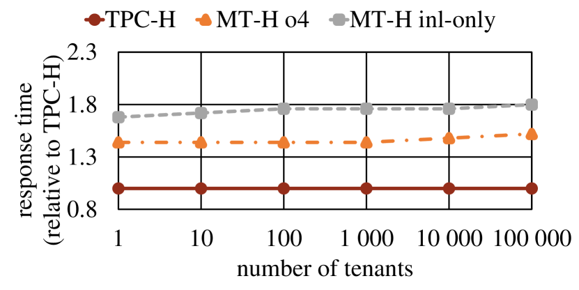
(a) MT-H Query 1

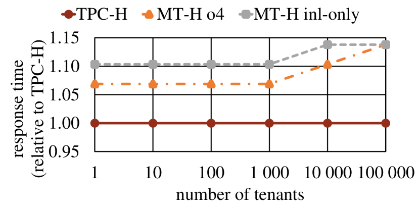
(b) MT-H Query 6

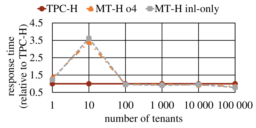
(c) MT-H Query 22

Figure 5: Response times (relative to TPC-H) of o4 and inlining-only optimization levels for selected MT-H queries, $sf=100$,
$T$ scaling from 1 to 100,000 on a log-scale, MTBase-on-PostgreSQL

Table 4 shows the MT-H queries for different optimization levels and Scenario 1 ($sf=1,T=10$) where client 1 queries her own data. As we can see, in that case, applying trivial optimizations in o1 is enough because these already eliminate all conversion functions and joins and only the D-filters remain. Executing these filters seems to be very inexpensive because most response times of the optimized queries are close to the baseline, TPC-H with $sf=0.1$. Queries 2, 11 and 16 however, take roughly ten times longer than the baseline. This is not surprising when taken into account that these queries only operate on shared tables which have ten times more data than in TPC-H. The same effect can be observed in Q09 where a significant part of the joined tables are shared.

Table 5 shows similar results, but for $D=2$, which means that now conversion functions can no longer be optimized away. While most of the queries show a similar behaviour than in the previous experiment, for the ones that involve a lot of conversion functions (i.e. queries 1, 6 and 22), we see how the performance becomes better with each optimization pass added. We also notice that while function inlining is very beneficial in general, it is even more so when combined with the other optimizations.

Finally, Table 6 shows the results where we query all data, i.e. $D=\{1,2,...,10\}$. This experiment involves even more conversion functions from all the different tenant formats into universal. In particular, when looking again at queries 1, 6 and 22, we observe the great benefit of conversion function distribution (added with optimization level o3), which, in turn, only works as great in conjunction with client and conversion function push-up because aggregation typically happens in the outermost query while conversion happens in the sub-queries. Overall, o4, which contains all optimization passes that MTBase offers, is the clear winner.

6.4 Cross-Tenant Query Processing at Large

In our final experiment, we evaluated the cost of cross-tenant query processing up to thousands of tenants. More concretely, we measured the response time of conversion-intensive MT-H queries (queries 1, 6 and 22) for a varying number of tenants between 1 and 100,000, for a large dataset where $sf=100$ and for the best optimization level (o4) as well as for inlining-only. The obtained results were then compared to plain TPC-H with $sf=100$, as shown in Figure 5. First of all, we notice that the cost overhead compared to single-tenant query-processing (TPC-H) stays below a factor of 2 and in general increases very moderately with the number of tenants. An interesting artifact can be observed for query 22 where MT-H for one tenant executes faster than plain TPC-H. The reason for this is a sub-optimal optimization decision in PostgreSQL: one of the most expensive parts of query 22, namely to find customers with a specific country code, is executed with a parallel scan in MT-H while no parallelism is used in the case of TPC-H.

7 Related Work

MTBase builds heavily on and extends a lot of related work. This section gives a brief summary of the most prominent lines of work that influenced our design.

Shared-resources (SR) systems: In related work, this approach is also often called database virtualization or database as a service (DaaS) when it is used in the cloud context. Important lines of work in this domain include (but are not limited to) SqlVM/Azure SQL DB [31, 18], RelationalCloud [30], SAP-HANA [35] and Snowflake [16], most of which is well summarized in [20]. MTBase complements these systems by providing a platform that can accommodate more, but typically smaller tenants.

Shared-databases (SD) systems: This approach, while appearing in the spectrum of multi-tenant databases by Chong et al. [15], is rare in practice. Sql Azure DB [18] seems to be the only product that has an implementation of this approach. However, even Microsoft strongly advises against using SD and instead recommends to either use SR or ST [29].

Shared-tables (ST) systems and schema evolution: work in that area includes Salesforce [38], Apache Phoenix [8], FlexScheme [10, 11] and Azure SQL Database [29]. Their common idea, as in MTSQL, is to use an invisible tenant identifier to identify which records belong to which tenant and rewrite SQL queries in order to include filters on this ttid. MTSQL extends these systems by providing the necessary features for cross-tenant query processing.

Database Federation/Data Integration: The importance of data integration and its connection to MTSQL was already stressed in the introduction. DI is often combined with database federation [27, 23], which means that there exist small program modules (called integrators, mediators or simply wrappers) to map data from different sources (possibly not all of them SQL databases) into one common format. While data federation generalizes well across the entire spectrum of multi-tenant databases, maintaining such wrapper architectures is expensive, both in terms of code maintenance and update processing. Conversely, MTSQL enables cross-tenant query processing in a more efficient and flexible way in the context of SS and ST databases.

Data Warehousing: Another approach how data integration can happen is during extract-transform-load (ETL) operations from different (OLTP) databases into a data warehouse [25]. Data warehouses have the well-known drawbacks that there are costly to maintain and that the data is possibly outdated [13, 32, 9]. Meanwhile, MTBase was specifically designed to work well in the context of integrated OLTP/OLAP systems, also known as hybrid transaction-analytical processing (HTAP) systems, and could therefore be advocated as in-situ or just-in-time data integration.

Security: How to compose our proposed system with tenant data encryption as proposed by Chong et al. [15] is not obvious as this opens the question how tenants can process data for which they have permission to process but which is owned by another tenant (and is therefore encrypted with that other tenant’s key). Obviously, simply sharing the key of tenant $t$ with all tenants that were granted the privilege to process $t$’s data is not a viable solution, as this allows them to impersonate $t$, which defeats the whole purpose of encryption. How to address this issue also depends a lot on the given attacker scenario: Do we want to protect tenants from each other? Do we trust the cloud provider? Do we expect honest-but-curious behaviour or active attacks? Also the granularity at which a tenant can share data with another tenant matters: schema- vs. table- vs. attribute- vs. row- vs. predicate-based, aggregations-only and possible combinations of these variants. For some of these granularities and attacker models, proposed solutions exist, e.g. in [19, 14].

8 Conclusion

This paper presented MTSQL, a novel paradigm to address cross-tenant query processing in multi-tenant databases. MTSQL extends SQL with multi-tenancy-aware syntax and semantics, which allows to efficiently optimize and execute cross-tenant queries in MTBase. MTBase is an open-source system that implements MTSQL. At its core, it is an MTSQL-to-SQL rewrite middleware sitting between a client and any DBMS of choice. The performance evaluation with a benchmark adapted from TPC-H showed that MTBase (on top of PostgeSQL) can scale to thousands of tenants at very low overhead and that our proposed optimizations to cross-tenant queries are highly effective.

In the future, we plan to further analyze the interplay between the MTBase query optimizer and its counter-part in the DBMS execution engine in order to assess the potential of cost-based optimizations. We also want to study conversion functions that vary over time and investigate how MTSQL can be extended to temporal databases. Moreover, we would like to look more into the privacy issues of multi-tenant databases, in particular how to enable cross-tenant query processing if data is encrypted.

Level	Q01	Q02	Q03	Q04	Q05	Q06	Q07	Q08	Q09	Q10	Q11	Q12	Q13	Q14	Q15	Q16	Q17	Q18	Q19	Q20	Q21	Q22
tpch-1G	0.8	0.053	0.1	0.077	0.18	0.067	0.13	0.12	0.28	0.092	0.078	0.1	0.66	0.095	0.1	0.19	0.071	0.25	0.072	5.2	0.21	0.04
canonical	1000	0.12	230	0.17	1.7	8.7	2.6	3.0	29	10	0.3	0.25	0.66	8.0	18	1.3	2.4	26	29	0.099	0.2	79
o1	0.78	0.1	0.23	0.14	0.087	0.099	0.95	0.15	1.1	0.12	0.29	0.25	0.65	0.14	0.14	1.3	0.13	8.9	0.91	0.076	0.19	0.55
o2	0.77	0.1	0.23	0.14	0.087	0.098	0.97	0.15	1.0	0.12	0.28	0.25	0.66	0.14	0.14	1.3	0.13	8.9	0.94	0.077	0.2	3.0
o3	0.78	0.1	0.23	0.14	0.088	0.097	0.93	0.15	1.1	0.12	0.28	0.25	0.65	0.14	0.14	1.3	0.14	8.8	0.92	0.078	0.2	3.1
o4	0.78	0.1	0.3	0.14	0.089	0.099	1.0	0.15	1.0	0.12	0.29	0.25	0.66	0.14	0.14	1.3	0.14	8.9	0.92	0.078	0.2	0.59
inl-only	0.78	0.1	0.24	0.14	0.088	0.097	0.95	0.15	1.0	0.12	0.29	0.25	0.67	0.14	0.14	1.3	0.14	8.9	0.91	0.076	0.2	0.55

Table 8: Response times [sec] of 22 TPC-H queries for MTBase-on-System-C with $sf=10$, $T=10$, $\rho=$ uniform, $C=1$,
$D=\{1\}$, for different levels of optimizations, versus TPC-H with $sf=1$

Level	Q01	Q02	Q03	Q04	Q05	Q06	Q07	Q08	Q09	Q10	Q11	Q12	Q13	Q14	Q15	Q16	Q17	Q18	Q19	Q20	Q21	Q22
tpch-1G	0.8	0.053	0.1	0.077	0.18	0.067	0.13	0.12	0.28	0.092	0.078	0.1	0.66	0.095	0.1	0.19	0.071	0.25	0.072	5.2	0.21	0.04
canonical	1100	0.13	240	0.18	1.6	9.0	1.8	2.7	29	10	0.29	0.25	0.66	7.9	18	1.3	2.3	26	28	0.12	0.2	80
o1	1100	0.12	250	0.16	1.6	9.0	1.8	2.9	30	11	0.29	0.25	0.68	7.9	18	1.3	2.4	26	29	0.13	0.19	80
o2	1100	0.11	240	0.18	1.6	8.9	14	2.9	40	10	0.29	0.25	0.67	7.8	18	1.3	2.2	26	28	0.11	0.2	80
o3	240	0.12	4.2	0.18	1.1	1.0	3.2	3.0	17	3.4	0.3	0.25	0.66	8.1	9.2	1.3	2.4	26	28	0.11	0.2	79
o4	1.1	0.1	0.17	0.14	0.15	0.099	0.91	0.16	0.94	2.1	0.31	0.25	0.67	0.34	0.29	1.3	0.15	1.5	1.1	0.089	0.2	1.2
inl-only	1.7	0.13	0.2	0.14	0.15	0.1	0.78	0.17	1.1	0.19	0.28	0.25	0.61	0.33	0.21	1.3	0.15	1.5	12	0.099	0.2	1.1

Table 9: Response times [sec] of 22 TPC-H queries for MTBase-on-System-C with $sf=10$, $T=10$, $\rho=$ uniform, $C=1$,
$D=\{2\}$, for different levels of optimizations, versus TPC-H with $sf=1$

Level	Q01	Q02	Q03	Q04	Q05	Q06	Q07	Q08	Q09	Q10	Q11	Q12	Q13	Q14	Q15	Q16	Q17	Q18	Q19	Q20	Q21	Q22
tpch-10G	7.9	0.097	0.94	0.81	1.6	0.83	0.92	0.68	2.5	0.85	0.27	1.1	5.5	0.92	0.9	1.3	0.7	2.6	0.76	0.14	2.0	0.32
canonical	11000	0.14	2500	1.7	28	90	20	38	200	1100	0.3	1.2	6.3	73	180	1.3	2.1	69	29	0.17	3.3	800
o1	11000	0.13	2500	1.6	28	90	21	37	190	1100	0.3	1.2	6.2	74	180	1.3	2.0	69	29	0.16	3.3	800
o2	11000	0.15	2400	1.7	29	90	24	39	310	1100	0.3	1.2	6.2	74	180	1.4	2.1	69	30	0.17	3.4	790
o3	2400	0.12	43	1.7	22	9.8	18	35	64	52	0.31	1.2	6.3	74	65	1.3	1.9	69	30	0.16	3.4	790
o4	38	0.13	1.1	1.6	0.59	0.97	1.6	1.2	5.3	29	0.31	1.2	6.2	1.1	2.4	1.3	0.83	11	1.3	0.14	3.4	0.75
inl-only	42	0.13	1.8	1.7	1.6	1.2	9.8	1.2	5.5	13	0.3	1.2	6.3	1.1	1.6	1.3	0.84	11	17	0.18	3.4	0.53

Table 10: Response times [sec] of 22 TPC-H queries for MTBase-on-System-C with $sf=10$, $T=10$, $\rho=$ uniform, $C=1$,
$D=\{1,2,...10\}$, for different levels of optimizations, versus TPC-H with $sf=10$

Appendix A More Rewriting Examples

While Section 3 of this paper focused on rewriting examples for queries, DDL and DML statements, which generally work very similarly, were only summarized briefly. In this paragraph we discuss some more elaborate examples.

A.1 Rewriting DDL statements

Section 3 already explained how to execute CREATE TABLE statements. Rewriting global constraints is also straight-forward: for global constraints, the ttids have to be made part of the constraint. For instance, the foreign key constraint of Listing 3 just becomes:

CONSTRAINT fk_emp FOREIGN KEY (E_role_id, ttid)
  REFERENCES Roles (R_role_id, ttid)

Tenant-specific check constraints are rewritten just like queries, so they automatically include the ttids where needed. The tricky question is how to implement tenant-specific referential integrity constraints. The way MTBase implements this, is to rewrite these constraints as check constraints. Imagine, as an example, that there is no global foreign key constraint on the Employees table and only tenant 0 adds this constraint privately. The way to rewrite this to a SQL check constraint is to make sure that the set of distinct keys in Employees_0 is a subset of the distinct keys in Roles_0:

CONSTRAINT fk_emp_0 CHECK (SELECT COUNT(E_role_id)
  FROM Employees WHERE ttid=0 AND E_role_id
    NOT IN (SELECT R_role_id FROM Roles
      WHERE ttid=0)) = 0

MTBase executes CREATE VIEW statements by rewriting their WHERE clause the same way it rewrites queries (including the proper dataset, $D$). No other modifications are needed.

A.2 Rewriting DML statements

INSERT statements that consist of a sub-query have to be executed in two steps: First, the sub-query is rewritten and executed on the DBMS on behalf of $C$. Second, for every $d\in D$, the result (which does not include any $ttid$s) is extended with $ttid=d$ before being executed on the DBMS as a simple INSERT statement that contains a simple list of VALUES.

For instance, consider tenant 0 inserting data on behalf of tenant 1 ($C=0,D=\{1\}$) with the following statement:

INSERT INTO Employees VALUES E_name, E_reg_id,
    E_salary, E_age (
    SELECT E_name, E_reg_id, E_salary, E_age
    FROM Employees WHERE E_age > 40
);

First of all, the intension of tenant 0 here is to copy some of his records over to tenant 1. The result of the SELECT sub-query, executed on behalf of tenant 0 on the exemplary database of Figure 2, is (’Alice’, 3, 150K, 46). This record is then converted into the format of tenant 1 and extended with its $ttid$: (1,’Alice’, 3, 135K, 46), before being inserted into the Employees table. This examples shows some of the difficulties of executing an INSERT (or UPDATE) statement on behalf of somebody else. First, as E_emp_id and E_role_id are NOT NULL, they must either have a default value or the statement fails. Second, for tenant 0 to provide a useful E_role_id for tenant 1 is difficult because it is a tenant-specific attribute. MTBase does not prevent a tenant from inserting tenant-specific attributes, even on behalf of other tenants, but it throws a warning in order to notify that the value might not make sense. Luckily, these problems do not occur with DELETE statements.

Appendix B Distributability Proof

In order to analyze how SUM and AVG distribute over linear functions, let us formally define the multi-set of values owned by tenant $t_{i}$ as $X_{i}$ and the corresponding (linear) conversion function as $f_{i}(x)=a_{i}x+b_{i}$.

As we will see first, the total average over all tenants (AVG) can be computed as the weighted average of the partial averages of the values of each tenant. This is proven by the following series of equations that starts with the total average on converted values and ends up with the weighted average of the converted partial averages:

$$\frac{\sum_{t\in T}\left({\sum_{x\in X_{t}}f_{t}(x)}\right)}{\sum_{t\in T}{|X_{t}|}}=\frac{\sum_{t\in T}\left({\sum_{x\in X_{t}}a_{t}x+b_{t}}\right)}{\sum_{t\in T}{|X_{t}|}}$$

$$=\frac{\sum_{t\in T}\left(a_{t}\left({\sum_{x\in X_{t}}x}\right)+b_{t}\cdot|X_{t}|\right)}{\sum_{t\in T}{|X_{t}|}}$$

$$=\frac{\sum_{t\in T}\left(\frac{|X_{t}|}{|X_{t}|}\left(a_{t}\left({\sum_{x\in X_{t}}x}\right)+b_{t}\cdot|X_{t}|\right)\right)}{\sum_{t\in T}{|X_{t}|}}$$

$$=\frac{\sum_{t\in T}\left(|X_{t}|\left(\frac{1}{|X_{t}|}\cdot a_{t}\left({\sum_{x\in X_{t}}x}\right)+b_{t}\right)\right)}{\sum_{t\in T}{|X_{t}|}}$$

$$=\frac{\sum_{t\in T}\left(|X_{t}|\cdot f\left(\frac{1}{|X_{t}|}\sum_{x\in X_{t}}x\right)\right)}{\sum_{t\in T}{|X_{t}|}}$$

If we look more carefully at these equations, we realize that the term below the fraction bar is always the same. This means that the set of equations, if we remove this term, also shows how the total sum can be computed by multiplying the partial averages with the corresponding partial counts, thereby proving that also SUM distributes over linear functions.

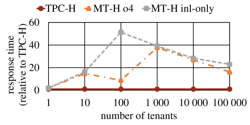
(a) MT-H Query 1

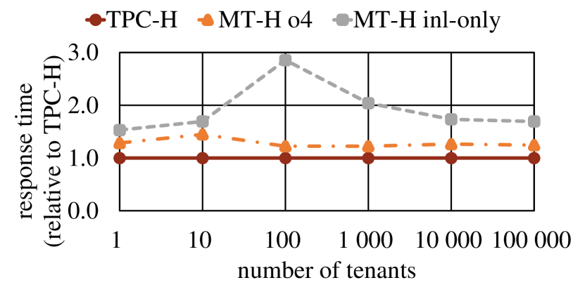
(b) MT-H Query 6

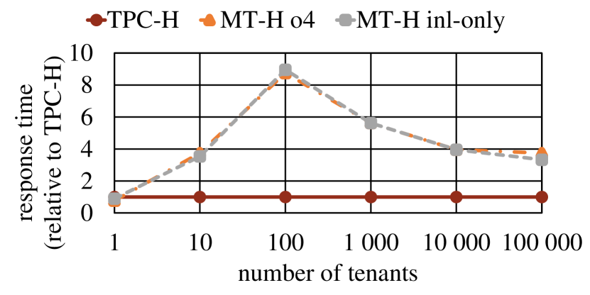
(c) MT-H Query 22

Figure 6: Response times (relative to TPC-H) of o4 and inlining-only optimization levels for selected MT-H queries, $sf=100$,
$T$ scaling from 1 to 100,000 on a log-scale, MTBase-on-System-C

Appendix C Optimizations on System C

As mentioned in Section 6, the performance numbers of MTBase on System C show, all in all, similar trends for optimization passes than to the ones on PostgreSQL. The only difference is that executing conversion functions (which are implemented as UDFs) is much more expensive in System C because results cannot be cached. As a consequence, executing queries without optimizations gets much worse and Q1 can take up to three hours to be processed on a 10 GB dataset. The results for scenario 1 are shown in Tables 8 to 10.

Appendix D Tenant Scaling on System C

An interesting picture can be seen for the tenant scaling experiment in Figure 6. While executing the queries for a small number of tenants ($\leq 10$) or a big one ($\geq 10,000$) seems to be reasonably cheap, executing queries for a mid-sized number of tenants seems to increase the costs dramatically. Looking at the query plans of System C did not reveal much because the plans are (probably intensionally) very coarse-grained. Thus, we can only speculate that for a mid-sized number of tenants, the optimizer does a couple of unfortunate decisions.

References

- [1] Python 2.7.2 Release. https://www.python.org/download/releases/2.7.2.
- [2] Scala Language. http://www.scala-lang.org.
- [3] TenantDB project page. *** Details omitted for double-blind reviewing ***.
- [4] TenantDB Rewrite Algorithm. *** Details omitted for double-blind reviewing ***.
- [5] The Glasgow Haskell Compiler. https://www.haskell.org/ghc.
- [6] The Java Database Connectivity (JDBC). http://www.oracle.com/technetwork/java/javase/jdbc/index.html.
- [7] Amazon Webservices. Amazon Relational Database Service (RDS). https://aws.amazon.com/rds.
- [8] Apache Foundation. Apache Phoenix: High performance relational database layer over HBase for low latency applicationsn - Multi-Tenancy Feature. http://phoenix.apache.org/multi-tenancy.html.
- [9] J. Arulraj, A. Pavlo, P. Menon, J. Arulraj, A. Pavlo, S. R. Dulloor, A. Pavlo, J. DeBrabant, J. Arulraj, A. Pavlo, et al. Bridging the Archipelago between Row-Stores and Column-Stores for Hybrid Workloads. In Proceedings of the 2016 ACM SIGMOD International Conference on Management of Data, volume 19, pages 57–63, 2016.
- [10] S. Aulbach, T. Grust, D. Jacobs, A. Kemper, and J. Rittinger. Multi-tenant databases for software as a service: schema-mapping techniques. In Proceedings of the 2008 ACM SIGMOD international conference on Management of data, pages 1195–1206. ACM, 2008.
- [11] S. Aulbach, M. Seibold, D. Jacobs, and A. Kemper. Extensibility and data sharing in evolving multi-tenant databases. In Data engineering (icde), 2011 ieee 27th international conference on, pages 99–110. IEEE, 2011.
- [12] H. Berenson, P. Bernstein, J. Gray, J. Melton, E. O’Neil, and P. O’Neil. A Critique of ANSI SQL Isolation Levels. SIGMOD Rec., 24(2):1–10, 1995.
- [13] L. Braun, T. Etter, G. Gasparis, M. Kaufmann, D. Kossmann, D. Widmer, A. Avitzur, A. Iliopoulos, E. Levy, and N. Liang. Analytics in Motion: High Performance Event-Processing AND Real-Time Analytics in the Same Database. In Proceedings of the 2015 ACM SIGMOD International Conference on Management of Data, pages 251–264. ACM, 2015.
- [14] J. M. A. Calero, N. Edwards, J. Kirschnick, L. Wilcock, and M. Wray. Toward a Multi-Tenancy Authorization System for Cloud Services. IEEE Security & Privacy, 8(6):48–55, 2010.
- [15] F. Chong, G. Carraro, and R. Wolter. Multi-tenant data architecture. MSDN Library, Microsoft Corporation, pages 14–30, 2006.
- [16] B. Dageville, T. Cruanes, M. Zukowski, V. Antonov, A. Avanes, J. Bock, J. Claybaugh, D. Engovatov, M. Hentschel, J. Huang, A. W. Lee, A. Motivala, A. Q. Munir, S. Pelley, P. Povinec, G. Rahn, S. Triantafyllis, and P. Unterbrunner. The Snowflake Elastic Data Warehouse. In Proceedings of the 2016 International Conference on Management of Data, SIGMOD Conference 2016, San Francisco, CA, USA, June 26 - July 01, 2016, pages 215–226, 2016.
- [17] S. Das, D. Agrawal, and A. El Abbadi. ElasTraS: An elastic, scalable, and self-managing transactional database for the cloud. ACM Transactions on Database Systems (TODS), 38(1):5, 2013.
- [18] S. Das, F. Li, V. R. Narasayya, and A. C. König. Automated Demand-driven Resource Scaling in Relational Database-as-a-Service. In Proceedings of the 2016 International Conference on Management of Data, SIGMOD Conference 2016, San Francisco, CA, USA, June 26 - July 01, 2016, pages 1923–1934, 2016.
- [19] S. D. C. Di Vimercati, S. Foresti, S. Jajodia, S. Paraboschi, and P. Samarati. Over-encryption: management of access control evolution on outsourced data. In Proceedings of the 33rd international conference on Very large data bases, pages 123–134. VLDB endowment, 2007.
- [20] A. J. Elmore, C. Curino, D. Agrawal, and A. El Abbadi. Towards database virtualization for database as a service. Proceedings of the VLDB Endowment, 6(11):1194–1195, 2013.
- [21] R. Fagin, L. M. Haas, M. Hernández, R. J. Miller, L. Popa, and Y. Velegrakis. Clio: Schema mapping creation and data exchange. In Conceptual Modeling: Foundations and Applications, pages 198–236. Springer, 2009.
- [22] J. Gray, S. Chaudhuri, A. Bosworth, A. Layman, D. Reichart, M. Venkatrao, F. Pellow, and H. Pirahesh. Data cube: A relational aggregation operator generalizing group-by, cross-tab, and sub-totals. Data mining and knowledge discovery, 1(1):29–53, 1997.
- [23] L. M. Haas, E. T. Lin, and M. A. Roth. Data integration through database federation. IBM Systems Journal, 41(4):578–596, 2002.
- [24] L. M. Haas, R. J. Miller, B. Niswonger, M. Tork Roth, P. M. Schwarz, and E. L. Wimmers. Transforming heterogeneous data with database middleware: Beyond integration. Data Engineering, page 31, 1999.
- [25] R. Kimball, M. Ross, et al. The data warehouse toolkit: the complete guide to dimensional modelling. Nachdr.]. New York [ua]: Wiley, pages 1–447, 2002.
- [26] S. Krishnan and J. L. U. Gonzalez. Google App Engine. In Building Your Next Big Thing with Google Cloud Platform, pages 83–122. Springer, 2015.
- [27] A. Levy. The information manifold approach to data integration. IEEE Intelligent Systems, 13(5):12–16, 1998.
- [28] S. M. Loesing. Architectures for elastic database services. PhD thesis, Diss., Eidgenössische Technische Hochschule ETH Zürich, Nr. 22441, 2015.
- [29] Microsoft Corporation. Microsoft Azure SQL Database. https://azure.microsoft.com/en-us/services/sql-database.
- [30] B. Mozafari, C. Curino, and S. Madden. DBSeer: Resource and Performance Prediction for Building a Next Generation Database Cloud. In CIDR, 2013.
- [31] V. R. Narasayya, S. Das, M. Syamala, B. Chandramouli, and S. Chaudhuri. SQLVM: Performance Isolation in Multi-Tenant Relational Database-as-a-Service. In CIDR, 2013.
- [32] T. Neumann, T. Mühlbauer, and A. Kemper. Fast serializable multi-version concurrency control for main-memory database systems. In Proceedings of the 2015 ACM SIGMOD International Conference on Management of Data, pages 677–689. ACM, 2015.
- [33] Oracle Corporation. ORACLE cloud. https://cloud.oracle.com/database.
- [34] V. Raman and J. M. Hellerstein. Potter’s wheel: An interactive data cleaning system. In VLDB, volume 1, pages 381–390, 2001.
- [35] SAP, November 2014. SAP HANA SPS 09 - What’s New? https://hcp.sap.com/content/dam/website/saphana/en_us/Technology%20Documents/SPS09/SAP%20HANA%20SPS%2009%20-%20Multitenant%20Database%20Cont.pdf.
- [36] Trasaction Processing Council. TPC-DI. http://www.tpc.org/tpcdi.
- [37] Trasaction Processing Council. TPC-H. http://www.tpc.org/tpch.
- [38] C. D. Weissman and S. Bobrowski. The design of the force. com multitenant internet application development platform. In SIGMOD Conference, pages 889–896, 2009.