Online Learning with Local Permutations and Delayed Feedback

Abstract

We propose an Online Learning with Local Permutations (OLLP) setting, in which the learner is allowed to slightly permute the order of the loss functions generated by an adversary. On one hand, this models natural situations where the exact order of the learner’s responses is not crucial, and on the other hand, might allow better learning and regret performance, by mitigating highly adversarial loss sequences. Also, with random permutations, this can be seen as a setting interpolating between adversarial and stochastic losses. In this paper, we consider the applicability of this setting to convex online learning with delayed feedback, in which the feedback on the prediction made in round $t$ arrives with some delay $\tau$. With such delayed feedback, the best possible regret bound is well-known to be $O(\sqrt{\tau T})$. We prove that by being able to permute losses by a distance of at most $M$ (for $M\geq\tau$), the regret can be improved to $O(\sqrt{T}(1+\sqrt{\tau^{2}/M}))$, using a Mirror-Descent based algorithm which can be applied for both Euclidean and non-Euclidean geometries. We also prove a lower bound, showing that for $M<\tau/3$, it is impossible to improve the standard $O(\sqrt{\tau T})$ regret bound by more than constant factors. Finally, we provide some experiments validating the performance of our algorithm.

1 Introduction

Online learning is traditionally posed as a repeated game where the learner has to provide predictions on an arbitrary sequence of loss functions, possibly even generated adversarially. Although it is often possible to devise algorithms with non-trivial regret guarantees, these have to cope with arbitrary loss sequences, which makes them conservative and in some cases inferior to algorithms not tailored to cope with worst-case behavior. Indeed, an emerging line of work considers how better online learning can be obtained on “easy” data, which satisfies some additional assumptions. Some examples include losses which are sampled i.i.d. from some distribution, change slowly in time, have a consistently best-performing predictor across time, have some predictable structure, mix adversarial and stochastic losses, etc. (e.g. Sani et al. (2014); Karnin and Anava (2016); Bubeck and Slivkins (2012); Seldin and Slivkins (2014); Hazan and Kale (2010); Chiang et al. (2012); Steinhardt and Liang (2014); Hazan and Kale (2011); Rakhlin and Sridharan (2013); Seldin and Slivkins (2014)).

In this paper, we take a related but different direction: Rather than explicitly excluding highly adversarial loss sequences, we consider how slightly perturbing them can mitigate their worst-case behavior, and lead to improved performance. Conceptually, this resembles smoothed analysis Spielman and Teng (2004), in which one considers the worst-case performance of some algorithm, after performing some perturbation to their input. The idea is that if the worst-case instances are isolated and brittle, then a perturbation will lead to easier instances, and better reflect the attainable performance in practice.

Specifically, we propose a setting, in which the learner is allowed to slightly reorder the sequence of losses generated by an adversary: Assuming the adversary chooses losses $h_{1},\ldots,h_{T}$, and before any losses are revealed, the learner may choose a permutation $\sigma$ on $\{1,\ldots,T\}$, satisfying $\max_{t}|t-\sigma(t)|\leq M$ for some parameter $M$, and then play a standard online learning game on losses $h_{\sigma(1)},\ldots,h_{\sigma(T)}$. We denote this as the Online Learning with Local Permutations (OLLP) setting. Here, $M$ controls the amount of power given to the learner: $M=0$ means that no reordering is performed, and the setting is equivalent to standard adversarial online learning. At the other extreme, $M=T$ means that the learner can reorder the losses arbitrarily. For example, the learner may choose to order the losses uniformly at random, making it a quasi-stochastic setting (the only difference compared to i.i.d. losses is that they are sampled without-replacement rather than with-replacement).

We argue that allowing the learner some flexibility in the order of responses is a natural assumption. For example, when the learner needs to provide rapid predictions on a high-frequency stream of examples, it is often immaterial if the predictions are not provided in the exact same order at which the examples arrived. Indeed, by buffering examples for a few rounds before being answered, one can simulate the local permutations discussed earlier.

We believe that this setting can be useful in various online learning problems, where it is natural to change a bit the order of the loss functions. In this paper, we focus on one well-known problem, namely online learning with delayed feedback. In this case, rather than being provided with the loss function immediately after prediction is made, the learner only receives the loss function after a certain number $\tau\geq 1$ of rounds. This naturally models situations where the feedback comes much more slowly than the required frequency of predictions: To give a concrete example, consider a web advertisement problem, where an algorithm picks an ad to display, and then receives a feedback from the user in the form of a click. It is likely that the algorithm will be required to choose ads for new users while still waiting for the feedback from the previous user.

For convex online learning with delayed feedback, in a standard adversarial setting, it is known that the attainable regret is on the order of $O(\sqrt{\tau T})$, and this is also the best possible in the worst case Weinberger and Ordentlich (2002); Mesterharm (2005); Langford et al. (2009); Joulani et al. (2013); Quanrud and Khashabi (2015). On the other hand, in a stochastic setting where the losses are sampled i.i.d. from some distribution, Agarwal and Duchi (2011) show that the attainable regret is much better, on the order of $O(\sqrt{T}+\tau)$. This gap between the worst-case adversarial setting, and the milder i.i.d. setting, hints that this problem is a good fit for our OLLP framework.

Thus, in this paper, we focus on online learning with feedback delayed up to $\tau$ rounds, in the OLLP framework where the learner is allowed to locally permute the loss functions (up to a distance of $M$). First, we devise an algorithm, denoted as Delayed Permuted Mirror Descent, and prove that it achieves an expected regret bound of order $O(\sqrt{T(\tau^{2}/M+1)})$ assuming $M\geq\tau$. As $M$ increases compared to $\tau$, this regret bound interpolates between the standard adversarial $\sqrt{\tau T}$ regret, and a milder $\sqrt{T}$ regret, typical of i.i.d. losses. As its name implies, the algorithm is based on the well-known online mirror descent (OMD) algorithm (see Hazan et al. (2016); Shalev-Shwartz et al. (2012)), and works in the same generality, involving both Euclidean and non-Euclidean geometries. The algorithm is based on dividing the entire sequence of functions into blocks of size $M$ and performing a random permutation within each block. Then, two copies of OMD are ran on different parts of each block, with appropriate parameter settings. A careful analysis, mixing adversarial and stochastic elements, leads to the regret bound.

In addition, we provide a lower bound complementing our upper bound analysis, showing that when $M$ is significantly smaller than $\tau$ (specifically, $\tau/3$), then even with local permutations, it is impossible to obtain a worse-case regret better than $\Omega(\sqrt{\tau T})$, matching (up to constants) the attainable regret in the standard adversarial setting where no permutations are allowed. Finally, we provide some experiments validating the performance of our algorithm.

The rest of the paper is organized as follows: in section 2 we formally define the Online Learning with Local Permutation setting, section 3 describes the Delayed Permuted Mirror Descent algorithm and outlines its regret analysis, section  4 discusses a lower bound for the delayed setting with limited permutation power, section 5 shows experiments, and finally section 6 provides concluding remarks, discussion, and open questions. Appendix A contains most of the proofs.

2 Setting and Notation

Convex Online Learning. Convex online learning is posed as a repeated game between a learner and an adversary (assumed to be oblivious in this paper). First, the adversary chooses $T$ convex losses $h_{1},\ldots,h_{T}$ which are functions from a convex set $\mathcal{W}$ to $\mathbb{R}$. At each iteration $t\in\{1,2,\ldots,T\}$, the learner makes a prediction $w_{t}$, and suffers a loss of $h_{t}\left(w_{t}\right)$. To simplify the presentation, we use the same notation $\nabla h_{t}(w)$ to denote either a gradient of $h_{t}$ at $w$ (if the loss is differentiable) or a subgradient at $w$ otherwise, and refer to it in both cases as a gradient. We assume that both $w\in\mathcal{W}$ and the gradients of any function $h_{t}$ in any point $w\in\mathcal{W}$ are bounded w.r.t. some norm: Given a norm $\|\cdot\|$ with a dual norm $\|\cdot\|_{\ast}$, we assume that the diameter of the space $\mathcal{W}$ is bounded by $B^{2}$ and that $\forall w\in\mathcal{W},\forall h\in\{h_{1},h_{2},...,h_{T}\}:\|\nabla h\left(w\right)\|_{\ast}\leq G$. The purpose of the learner is to minimize her (expected) regret, i.e.

$$R(T)=\mathbb{E}\left[\sum_{t=1}^{T}h_{t}\left(w_{t}\right)-\sum_{t=1}^{T}h_{t}\left(w^{\ast}\right)\right]~{}~{}~{}~{}\text{where}~{}~{}~{}~{}w^{\ast}=\underset{w\in\mathcal{W}}{\text{argmin }}\sum_{t=1}^{T}h_{t}\left(w\right)$$

where the expectation is with respect to the possible randomness of the algorithm.

Learning with Local Permutations. In this paper, we introduce and study a variant of this standard setting, which gives the learner a bit more power, by allowing her to slightly modify the order in which the losses are processed, thus potentially avoiding highly adversarial but brittle loss constructions. We denote this setting as the Online Learning with Local Permutations (OLLP) setting. Formally, letting $M$ be a permutation window parameter, the learner is allowed (at the beginning of the game, and before any losses are revealed) to permute $h_{1},\ldots,h_{T}$ to $h_{\sigma^{-1}(1)},\ldots,h_{\sigma^{-1}(T)}$, where $\sigma$ is a permutation from the set $Perm:=\left\{\sigma:\forall t,|\sigma\left(t\right)-t|\leq M\right\}$. After this permutation is performed, the learner is presented with the permuted sequence as in the standard online learning setting, with the same regret as before. To simplify notation, we let $f_{t}=h_{\sigma^{-1}(t)}$, so the learner is presented with the loss sequence $f_{1},\ldots,f_{T}$, and the regret is the same as the standard regret, i.e. $R(T)=\mathbb{E}\left[\sum_{t=1}^{T}f_{t}(w_{t})-\sum_{t=1}^{T}f_{t}(w^{*})\right]$. Note that if $M=0$ then we are in the fully adversarial setting (no permutation is allowed). At the other extreme, if $M=T$ and $\sigma$ is chosen uniformly at random, then we are in a stochastic setting, with a uniform distribution over the set of functions chosen by the adversary (note that this is close but differs a bit from a setting of i.i.d. losses). In between, as $M$ varies, we get an interpolation between these two settings.

Learning with Delayed Feedback. The OLLP setting can be useful in many applications, and can potentially lead to improved regret bounds for various tasks, compared to the standard adversarial online learning. In this paper, we focus on studying its applicability to the task of learning from delayed feedback.

Whereas in standard online learning, the learner gets to observe the loss $f_{t}$ immediately at the end of iteration $t$, here we assume that at round $t$, she only gets to observe $f_{t-\tau}$ for some delay parameter $\tau<T$ (and if $t<\tau$, no feedback is received). For simplicity, we focus on the case where $\tau$ is fixed, independent of $t$, although our results can be easily generalized (as discussed in subsection 3.3). We emphasize that this is distinct from another delayed feedback scenario sometimes studied in the literature (Agarwal and Duchi (2011); Langford et al. (2009)), where rather than receiving $f_{t-\tau}$ the learner only receives a (sub)gradient of $f_{t-\tau}$ at $w_{t-\tau}$. This is a more difficult setting, which is relevant for instance when the delay is due to the time it takes to compute the gradient.

3 Algorithm and Analysis

Our algorithmic approach builds on the well-established online mirror descent framework. Thus, we begin with a short reminder of the Online Mirror Descent algorithm (see e.g. Hazan et al. (2016) for more details). Readers who are familiar with the algorithm are invited to skip to Subsection 3.1.

The online mirror descent algorithm is a generalization of online gradient descent, which can handle non-Euclidean geometries. The general idea is the following: we start with some point $w_{t}\in\mathcal{W}$, where $\mathcal{W}$ is our primal space. We then map this point to the dual space using a (striclty convex and continuously differentiable) mirror map $\psi$, i.e. $\nabla\psi\left(w_{t}\right)\in\mathcal{W}^{\ast}$, then perform the gradient update in the dual space, and finally map the resulting new point back to our primal space $\mathcal{W}$ again, i.e. we want to find a point $w_{t+1}\in\mathcal{W}$ s.t. $\nabla\psi\left(w_{t+1}\right)=\nabla\psi\left(w_{t}\right)-\eta\cdot g_{t}$ where $g_{t}$ denotes the gradient. Denoting by $w_{t+\frac{1}{2}}$ the point satisfying $\nabla\psi(w_{t+\frac{1}{2}})=\nabla\psi\left(w_{t}\right)-\eta\cdot g_{t}$, it can be shown that $w_{t+\frac{1}{2}}=\left(\nabla\psi^{\ast}\right)\left(\nabla\psi\left(w_{t}\right)-\eta\cdot g_{t}\right)$, where $\psi^{\ast}$ is the dual function of $\psi$. This point, $w_{t+\frac{1}{2}}$, might lie outside our hypothesis class $\mathcal{W}$, and thus we might need to project it back to our space $\mathcal{W}$. We use the Bregman divergence associated to $\psi$ to do this:

$$w_{t+1}=\underset{w\in\mathcal{W}}{argmin}\triangle_{\psi}(w,w_{t+\frac{1}{2}}),$$

where the Bregman divergence $\Delta_{\psi}$ is defined as

$$\triangle_{\psi}\left(x,y\right)=\psi\left(x\right)-\psi\left(y\right)-\langle\nabla\psi(y),x-y\rangle.$$

Specific choices of the mirror map $\psi$ leads to specific instantiations of the algorithms for various geometries. Perhaps the simplest example is $\psi\left(x\right)=\frac{1}{2}\|x\|_{2}^{2}$, with associated Bregman divergence $\triangle_{\psi}\left(x,y\right)=\frac{1}{2}\cdot\|x-y\|^{2}$. This leads us to the standard and well-known online gradient descent algorithm, where $w_{t+1}$ is the Euclidean projection on the set $\mathcal{W}$ of $w_{t}-\eta\cdot g_{t}$.

Another example is the negative entropy mirror map $\psi\left(x\right)=\sum_{i=1}^{n}x_{i}\cdot\log\left(x_{i}\right)$, which is $1$-strongly convex with respect to the $1$-norm on the simplex $\mathcal{W}=\left\{x\in\mathbb{R}^{n}_{+}:\sum_{i=1}^{n}x_{i}=1\right\}$. In that case, the resulting algorithm is the well-known multiplicative updates algorithm, where $w_{t+1,i}=w_{t,i}\cdot\exp(-\eta g_{t,i})/\sum_{j=1}^{n}w_{t,i}\cdot\exp(-\eta g_{t,j})$. Instead of the $1$-norm on the simplex, one can also consider arbitrary $p$-norms, and take $\psi(x)=\frac{1}{2}\cdot\|x\|_{q}^{2}$, where $q$ is the dual norm (satisfying $1/p+1/q=1$).

3.1 The Delayed Permuted Mirror Descent Algorithm

Before describing the algorithm, we note that we will focus here on the case where the permutation window parameter $M$ is larger than the delay parameter $\tau$. If $M<\tau$, then our regret bound is generally no better than the $O(\sqrt{\tau T})$ obtainable by a standard algorithm without any permutations, and for $M<\tau/3$, this is actually tight as shown in Section 4.

We now turn to present our algorithm, denoted as The Delayed Permuted Mirror Descent algorithm (see algorithm 1 below as well as figure 1 for a graphical illustration). First, the algorithm splits the time horizon $T$ into $M$ consecutive blocks, and performs a uniformly random permutation on the loss functions within each block. Then, it runs two online mirror descent algorithms in parallel, and uses the delayed gradients in order to update two separate predictors – $w^{f}$ and $w^{s}$, where $w^{f}$ is used for prediction in the first $\tau$ rounds of each block, and $w^{s}$ is used for prediction in the remaining $M-\tau$ rounds (here, $f$ stands for “first” and $s$ stands for “second”). The algorithm maintaining $w^{s}$ crucially relies on the fact that the gradient of any two functions in a block (at some point $w$) is equal, in expectation over the random permutation within each block. This allows us to avoid most of the cost incurred by delays within each block, since the expected gradient of a delayed function and the current function are equal. A complicating factor is that at the first $\tau$ rounds of each block, no losses from the current block has been revealed so far. To tackle this, we use another algorithm (maintaining $w^{f}$), specifically to deal with the losses at the beginning of each block. This algorithm does not benefit from the random permutation, and its regret scales the same as standard adversarial online learning with delayed feedback. However, as the block size $M$ increases, the proportion of losses handled by $w^{f}$ decreases, and hence its influence on the overall regret diminishes.

The above refers to how the blocks are divided for purposes of prediction. For purposes of updating the predictor of each algorithm, we need to use the blocks a bit differently. Specifically, we let $T_{1}$ and $T_{2}$ be two sets of indices. $T_{1}$ includes all indices from the first $\tau$ time points of every block, and is used to update $w^{f}$. $T_{2}$ includes the first $M-\tau$ indices of every block, and is used to update $w^{s}$ (see figure 1). Perhaps surprisingly, note that $T_{1}$ and $T_{2}$ are not disjoint, and their union does not cover all of $\{1,\ldots,T\}$. The reason is that due to the random permutation in each block, the second algorithm only needs to update on some of the loss functions in each block, in order to obtain an expected regret bound on all the losses it predicts on.

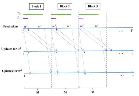
Figure 1: Scheme of predictions and updates of both parallel algorithms (best viewed in color; see text for details). Top color bars mark which iterations are in $T_{1}$ (purple lines) and which are in $T_{2}$ (green lines). Top timeline shows which predictor, $w^{f}$ or $w^{s}$, is used to predict in each iteration. Middle timeline shows where gradients for updating $w^{f}$ come from (first $\tau$ iterations of the previous block), and lower timeline shows where gradients for updating $w^{s}$ come from (first $M-\tau$ iterations of the same block, each gradient from exactly $\tau$ rounds back).

Algorithm 1 Delayed Permuted Mirror Descent

  Input: $M$, $\eta_{f}$, $\eta_{s}$

  Init: $w_{1}^{f}=0$, $w_{1}^{s}=0$, $j_{f}=j_{s}=1$

  Divide $T$ to consecutive blocks of size $M$, and permute the losses uniformly at random within each block. Let $f_{1},\ldots,f_{T}$ denote the resulting permuted losses.

  for $t=1...,T$ do

     if  $t\in$ first $\tau$ rounds of the block then

        Predict using $w_{j_{f}}^{f}$

        Receive a loss function from $\tau$ places back: $f_{t-M}=f_{T_{1}\left(j_{f}-\tau\right)}$. If none exists (in the first $\tau$ iterations), take the $0$ function.

        Compute: $\nabla f_{T_{1}\left(j_{f}-\tau\right)}\left(w_{j_{f}-\tau}^{f}\right)$

        Update: $w_{j_{f}+\frac{1}{2}}^{f}=\left(\nabla\psi^{\ast}\right)\left(\nabla\psi\left(w_{j_{f}}^{f}\right)-\eta_{f}\nabla f_{T_{1}\left(j_{f}-\tau\right)}\left(w_{j_{f}-\tau}^{f}\right)\right)$

        Project: $w_{j_{f}+1}=\underset{w\in\mathcal{W}}{argmin}\triangle_{\psi}\left(w,w_{j_{f}+\frac{1}{2}}^{f}\right)$ $j_{f}=j_{f}+1$

     else

        Predict using $w_{j_{s}}^{s}$

        Receive a loss function from $\tau$ places back: $f_{t-\tau}=f_{T_{2}\left(j_{s}\right)}$

        Compute: $\nabla f_{t-\tau}\left(w_{j_{s}}^{s}\right)=\nabla f_{T_{2}\left(j_{s}\right)}\left(w_{j_{s}}^{s}\right)$

        Update: $w_{j_{s}+\frac{1}{2}}^{s}=\left(\nabla\psi^{\ast}\right)\left(\nabla\psi\left(w_{j_{s}}^{s}\right)-\eta_{s}\cdot\nabla f_{T_{2}\left(j_{s}\right)}\left(w_{j_{s}}^{s}\right)\right)$

        Project: $w_{j_{s}+1}=\underset{w\in\mathcal{W}}{argmin}\triangle_{\psi}\left(w,w_{j_{s}+\frac{1}{2}}^{s}\right)$ $j_{s}=j_{s}+1$

     end if

  end for

3.2 Analysis

The regret analysis of the Delayed Permuted Mirror Descent algorithm is based on a separate analysis of each of the two mirror descent sub-algorithms, where in the first sub-algorithm the delay parameter $\tau$ enters multiplicatively, but doesn’t play a significant role in the regret of the second sub-algorithm (which utilizes the stochastic nature of the permutations). Combining the regret bound of the two sub-algorithms, and using the fact that the portion of losses predicted by the second algorithm increases with $M$, leads to an overall regret bound improving in $M$.

In the proof, to analyze the effect of delay, we need a bound on the distance between any two consequent predictors $w_{t},w_{t+1}$ generated by the sub-algorithm. This depends on the mirror map and Bregman divergence used for the update, and we currently do not have a bound holding in full generality. Instead, we let $\Psi_{(\eta_{f},G)}$ be some upper bound on $\|w_{t+1}-w_{t}\|$, where the update is using step-size $\eta_{f}$ and gradients of norm $\leq G$. Using $\Psi_{\left(\eta_{f},G\right)}$ we prove a general bound for all mirror maps. In Lemmas 3 and 4 in Appendix A.1, we show that for two common mirror maps (corresponding to online gradient descent and multiplicative weights), $\Psi_{(\eta_{f},G)}\leq c\cdot\eta_{f}G$ for some numerical constant $c$, leading to a regret bound of $O(\sqrt{T(\tau^{2}/M+1)})$. Also, we prove theorem 1 for $1$-strongly convex mirror maps, although it can be generalized to any $\lambda$-strongly convex mirror map by scaling.

Theorem 1.

Given a norm $\|\cdot\|$, suppose that we run the Delayed Permuted Mirror Descent algorithm using a mirror map $\psi$ which is $1$-strongly convex w.r.t. $\|\cdot\|$, over a domain $\mathcal{W}$ with diameter $B^{2}$ w.r.t the bregman divergence of $\psi$: $\forall w,v\in\mathcal{W}:\triangle_{\psi}(w,v)\leq B^{2}$, and such that the (sub)-gradient $g$ of each loss function on any $w\in\mathcal{W}$ satisfies $\|g\|_{*}\leq G$ (where $\|\cdot\|_{*}$ is the dual norm of $\|\cdot\|$). Then the expected regret, given a delay parameter $\tau$ and step sizes $\eta_{f},\eta_{s}$ satisfies:

$$\mathbb{E}\left[\sum_{t=1}^{T}f_{t}\left(w_{t}\right)-f_{t}\left(w^{\ast}\right)\right] \leq\frac{B^{2}}{\eta_{f}}+\eta_{f}\cdot\frac{T\tau}{M}\cdot\frac{G^{2}}{2}+\frac{T\tau^{2}}{M}\cdot G\cdot\Psi_{\left(\eta_{f},G\right)}+\frac{B^{2}}{\eta_{s}}+\eta_{s}\cdot\frac{T\cdot\left(M-\tau\right)}{M}\cdot\frac{G^{2}}{2}$$

Furthermore, if $\Psi_{\left(\eta_{f},G\right)}\leq c\cdot\eta_{f}G$ for some constant $c$, and $\eta_{f}=\frac{B\cdot\sqrt{M}}{G\cdot\sqrt{T\cdot\tau\cdot\left(\frac{1}{2}+c\cdot\tau\right)}}$, $\eta_{s}=\frac{B\cdot\sqrt{2M}}{G\cdot\sqrt{T\cdot\left(M-\tau\right)}}$, the regret is bounded by

$$c\sqrt{\frac{T\tau}{M}}\cdot BG\sqrt{\frac{1}{2}+c\cdot\tau}+\sqrt{\frac{2T\left(M-\tau\right)}{M}}\cdot BG~{}=~{}\mathcal{O}\left(\sqrt{T}\cdot\left(\sqrt{\frac{\tau^{2}}{M}}+1\right)\right)$$

When $M=\mathcal{O}(\tau)$, this bound is $O(\sqrt{\tau T})$. similar to the standard adversarial learning case. However, as $M$ increases, the regret gradually improves to $O(\sqrt{T}+\tau)$, which is the regret attainable in a purely stochastic setting with i.i.d. losses. The full proof can be found in appendix A.1.1, and we sketch below the main ideas.

First, using the definition of regret, we show that it is enough to upper-bound the regret of each of the two sub-algorithms separately. Then, by a standard convexity argument, we reduce this to bounding sums of terms of the form $\mathbb{E}[\langle w^{f}_{t}-w_{f}^{\ast},\nabla f_{t}(w^{f}_{t})\rangle]$ for the first sub-algorithm, and $\mathbb{E}\left[\langle w^{s}_{t}-w_{s}^{\ast},\nabla f_{t}\left(w^{s}_{t}\right)\rangle\right]$ for the second sub-algorithm (where $w^{\ast}_{f}$ and $w_{s}^{\ast}$ are the best fixed points in hindsight for the losses predicted on by the first and second sub-algorithms, respectively, and where for simplicity we assume the losses are differentiable). In contrast, we can use the standard analysis of mirror descent, using delayed gradients, to get a bound for the somewhat different terms $\mathbb{E}[\langle w^{f}_{t}-w_{f}^{\ast},\nabla f_{t-\tau}(w^{f}_{t-\tau})\rangle]$ for the first sub-algorithm, and $\mathbb{E}\left[\langle w^{s}_{t}-w_{s}^{\ast},\nabla f_{t-\tau}\left(w^{s}_{t}\right)\rangle\right]$ for the second sub-algorithm. Thus, it remains to bridge between these terms.

Starting with the second sub-algorithm, we note that since we performed a random permutation within each block, the expected value of all loss functions within a block (in expectation over the block, and evaluated at a fixed point) is equal. Moreover, at any time point, the predictor $w^{s}$ maintained by the second sub-algorithm does not depend on the delayed nor the current loss function. Therefore, conditioned on $w^{s}_{t}$, and in expectation over the random permutation in the block, we have that

$$\mathbb{E}[\nabla f_{t}(w_{t}^{s})]=\mathbb{E}[f_{t-\tau}(w_{t}^{s})]$$

from which it can be shown that

$$\mathbb{E}\left[\langle w^{s}_{t}-w_{s}^{\ast},\nabla f_{t}(w^{s}_{t})\rangle\right]=\mathbb{E}\left[\langle w^{s}_{t}-w_{s}^{\ast},\nabla f_{t-\tau}(w^{s}_{t})\rangle\right]$$

Thus, up to a negligible factor having to do with the first few rounds of the game, the second sub-algorithm’s expected regret does not suffer from the delayed feedback.

For the first sub-algorithm, we perform an analysis which does not rely on the random permutation. Specifically, we first show that since we care just about the sum of the losses, it is sufficient to bound the difference between $\mathbb{E}[\langle w^{f}_{t}-w_{f}^{\ast},\nabla f_{t}(w^{f}_{t})\rangle]$ and $\mathbb{E}[\langle w^{f}_{t+\tau}-w_{f}^{\ast},\nabla f_{t}(w^{f}_{t})\rangle]$. Using Cauchy-Shwartz, this difference can be upper bounded by $\|w_{t}^{f}-w_{t+\tau}^{f}\|\cdot\|\nabla f_{t}(w^{f}_{t})\|$, which in turn is at most $c\cdot\tau\cdot\eta_{f}\cdot G^{2}$ using our assumptions on the gradients of the losses and the distance between consecutive predictors produced by the first sub-algorithm.

Overall, we get two regret bounds, one for each sub-algorithm. The regret of the first sub-algorithm scales with $\tau$, similar to the no-permutation setting, but the sub-algorithm handles only a small fraction of the iterations (the first $\tau$ in every block of size $M$). In the rest of the iterations, where we use the second sub-algorithm, we get a bound that resembles more the stochastic case, without such dependence on $\tau$. Combining the two, the result stated in Theorem 1 follows.

3.3 Handling Variable Delay Size

So far, we discussed a setting where the feedback arrives with a fixed delay of size $\tau$. However, in many situations the feedback might arrive with a variable delay size $\tau_{t}$ at any iteration $t$, which may raise a few issues. First, feedback might arrive in an asynchronous fashion, causing us to update our predictor using gradients from time points further in past after already using more recent gradients. This complicates the analysis of the algorithm. A second, algorithmic problem, is that we could also possibly receive multiple feedbacks simultaneously, or no feedback at all, in certain iterations, since the delay is of variable size. One simple solution is to use buffering and reduce the problem to a constant delay setting. Specifically, we assume that all delays are bounded by some maximal delay size $\tau$. We would like to use one gradient to update our predictor at every iteration (this is mainly for ease of analysis, practically one could update the predictor with multiple loss functions in a single iteration). In order to achieve this, we can use a buffer to store loss functions that were received but have not been used to update the predictors yet. We define $Grad_{f}$ and $Grad_{s}$, two buffers that will contain gradients from time points in $T_{1}$ or $T_{2}$, correspondingly. Each buffer is of size $\tau$. If we denote by $\mathcal{F}_{t}$ the set of function that have arrived in time $t$, we can simply store loss functions that have arrived asynchronously in the buffers defined above, sort them in ascending order, and take the delayed loss function from exactly $\tau$ iterations back in the update step. This loss function must be in the appropriate buffer since the maximal delay size is $\tau$. From this moment on, the algorithm can proceed as usual and its analysis still applies.

4 Lower Bound

In this section, we give a lower bound in the setting where $M<\frac{\tau}{3}$ with all feedback having delay of exactly $\tau$. We will show that for this case, the regret bound cannot be improved by more than a constant factor over the bound of the adversarial online learning problem with a fixed delay of size $\tau$, namely $\Omega\left(\sqrt{\tau T}\right)$ for a sequence of length $T$. We hypothesize that this regret bound also cannot be significantly improved for any $M=O(\tau)$ (and not just $\tau/3$). However, proving this remains an open problem.

Theorem 2.

For every (possible randomized) algorithm $A$ with a permutation window of size $M\leq\frac{\tau}{3}$, there exists a choice of linear, $1$-Lipschitz functions over $[-1,1]\subset\mathbb{R}$, such that the expected regret of $A$ after $T$ rounds (with respect to the algorithm’s randomness), is

$$\mathbb{E}\left[\sum_{t=1}^{T}f_{t}\left(w_{t}\right)-\sum_{t=1}^{T}f_{t}\left(w^{\ast}\right)\right]=\Omega\left(\sqrt{\tau T}\right)~{}~{}~{}~{}\text{where }~{}~{}~{}~{}w^{\ast}=\underset{w\in\mathcal{W}}{\text{argmin }}\sum_{t=1}^{T}f_{t}\left(w\right)$$

For completeness, we we also provide in appendix A.2 a proof that when $M=0$ (i.e. no permutations allowed), then the worst-case regret is no better than $\Omega(\sqrt{\tau T})$. This is of course a special case of Theorem 2, but applies to the standard adversarial online setting (without any local permutations), and the proof is simpler. The proof sketch for the setting where no permutation is allowed was already provided in Langford et al. (2009), and our contribution is in providing a full formal proof.

The proof in the case where $M=0$ is based on linear losses of the form $f_{t}=\alpha_{t}\cdot w_{t}$ over $[-1,+1]$, where $\alpha_{t}\in\{-1,+1\}$. Without permutations, it is possible to prove a $\Omega(\sqrt{\tau T})$ lower bound by dividing the $T$ iterations into blocks of size $\tau$, where the $\alpha$ values of all losses at each block is the same and randomly chosen to equal either $+1$ or $-1$. Since the learner does not obtain any information about this value until the block is over, this reduces to adversarial online learning over $T/\tau$ rounds, where the regret at each round scales linearly with $\tau$, and overall regret at least $\Omega(\tau\sqrt{T/\tau})=\Omega(\sqrt{\tau T})$.

In the proof of theorem 2, we show that by using a similar construction, even with permutations, having a permutation window less than $\tau/3$ still means that the $\alpha$ values would still be unknown until all loss functions of the block are processed, leading to the same lower bound up to constants.

The formal proof appears in the appendix, but can be sketched as follows: first, we divide the $T$ iterations into blocks of size $\tau/3$. Loss functions within each block are identical, of the form $f_{t}=\alpha_{t}\cdot w_{t}$, and the value of $\alpha$ per block is chosen uniformly at random from $\{-1,+1\}$, as before. Since here, the permutation window $M$ is smaller than $\tau/3$, then even after permutation, the time difference between the first and last time we encounter an $\alpha$ that originated from a single block is less than $\tau$. This means that by the time we get any information on the $\alpha$ in a given block, the algorithm already had to process all the losses in the block, which leads to the same difficulty as the no-permutation setting. Specifically, since the predictors chosen by the algorithm when handling the losses of the block do not depend on the $\alpha$ value in that block, and that $\alpha$ is chosen randomly, we get that the expected loss of the algorithm at any time point $t$ equals $0$. Thus, the cumulative loss across the entire loss sequence is also $0$. In contrast, for $w^{\ast}$, the optimal predictor in hindsight over the entire sequence, we can prove an expected accumulated loss of $-\Omega(\sqrt{\tau T})$ after $T$ iterations, using Khintchine inequality and the fact that the $\alpha$’s were randomly chosen per block. This leads us to a lower bound of expected regret of order $\sqrt{\tau T}$, for any algorithm with a local permutation window of size $M<\tau/3$.

5 Experiments

We consider the adversarial setting described in section 4, where an adversary chooses a sequence of functions such that every $\tau$ functions are identical, creating blocks of size $\tau$ of identical loss functions, of the form $f_{t}(w_{t})=\alpha_{t}\cdot w_{t}$ where $\alpha_{t}$ is chosen randomly in $\{-1,+1\}$ for each block. In all experiments we use $T=10^{5}$ rounds, a delay parameter of $\tau=200$, set our step sizes according to the theoretical analysis, and report the mean regret value over 1000 repetitions of the experiments.

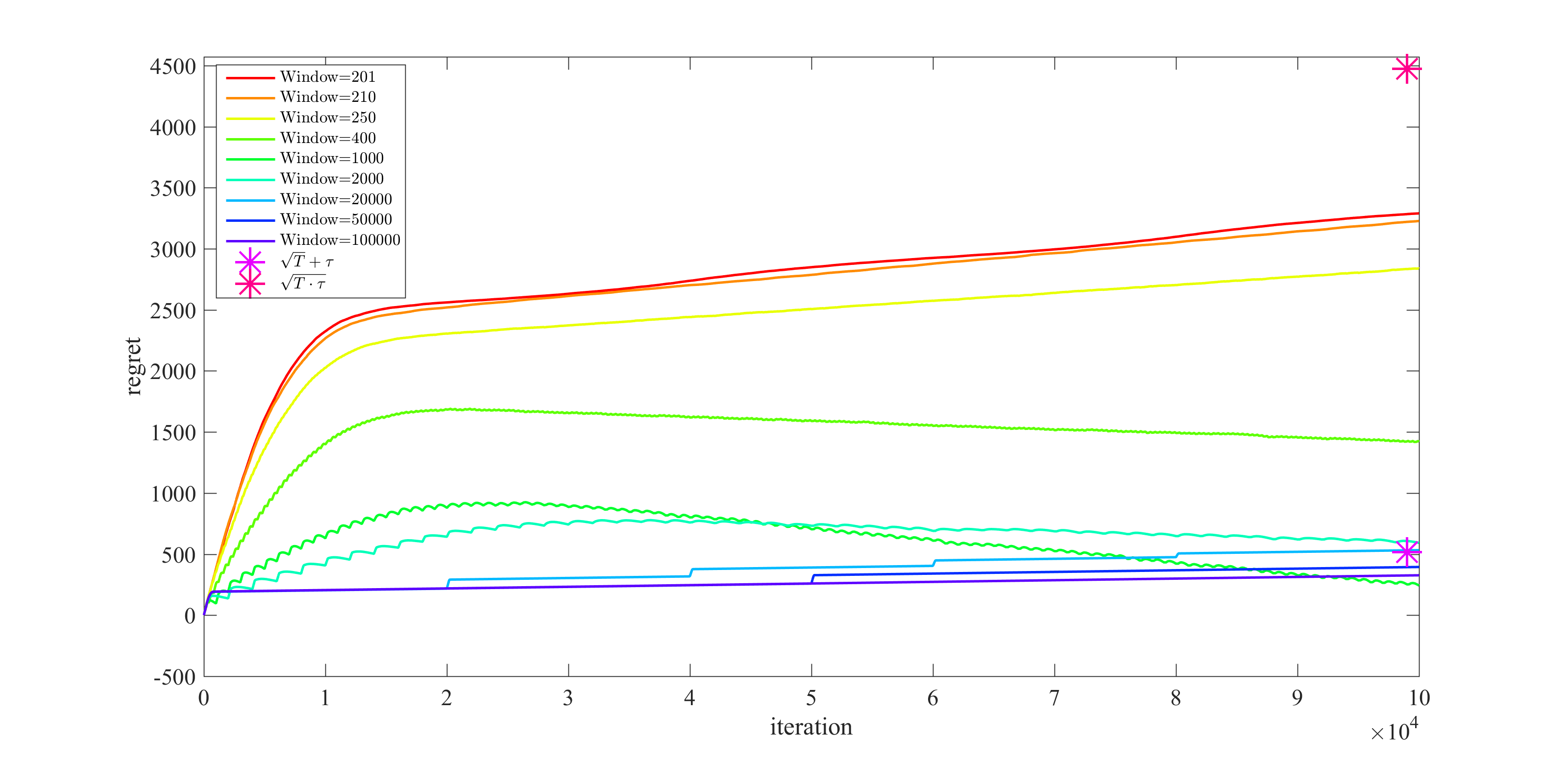
Figure 2: Regret of the Delayed Permuted Mirror Descent algorithm, with local permutation in window sizes ranging from $M=\tau+1$ to $M=T$. A pink $\ast$ indicates the order of the stochastic bound ($\sqrt{T}+\tau$), and a red $\ast$ indicates the order of the adversarial bound ($\sqrt{\tau T}$). Regret is averaged over 1000 repetitions. Best viewed in color.

In our first experiment, we considered the behavior of our Delayed Permuted Mirror Descent algorithm, for window sizes $M>\tau$, ranging from $\tau+1$ to $T$. In this experiment, we chose the $\alpha$ values randomly, while ensuring a gap of 200 between the number of blocks with $+1$ values and the number of blocks with $-1$ values (this ensures that the optimal $w^{\ast}$ is a sufficiently strong competitor, since otherwise the setting is too “easy” and the algorithm can attain negative regret in some situations). The results are shown in Figures 2 and 3, where the first figure presents the accumulated regret of our algorithm over time, whereas the second figure presents the overall regret after $T$ rounds, as a function of the window size $M$.

When applying our algorithm in this setting with different values of $M>\tau$, ranging from $M=\tau+1$ and up to $M=T$, we get a regret that scales from the order of the adversarial bound to the order of the stochastic bound depending on the window size, as expected by our analysis. For all window sizes greater than $5\cdot\tau$, we get a regret that is in the order of the stochastic bound - this is not surprising, since after the permutation we get a sequence of functions that is very close to an i.i.d. sequence, in which case any algorithm can be shown to achieve $O(\sqrt{T})$ regret in expectation. Note that this performance is better than that predicted by our theoretical analysis, which implies an $O(\sqrt{T})$ behavior only when $M\geq\Omega(\tau^{2})$. It is an open and interesting question whether it means that our analysis can be improved, or whether there is a harder construction leading to a tighter lower bound.

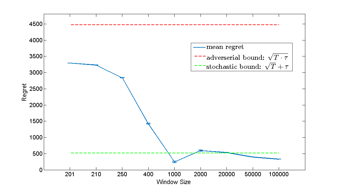
Figure 3: Regret of the Delayed Permuted Mirror Descent algorithm for different window sizes, after $T=10^{5}$ iterations, with local permutation window sizes ranging from $M=\tau+1$ to $M=T$. Red dashed line (top) indicates the order of the adversarial bound ($\sqrt{\tau T}$) and green dashed line (bottom) indicates the order of the stochastic bound ($\sqrt{T}+\tau$). Regret is averaged over 1000 repetitions, error bars indicate standard error of the mean. Best viewed in color.

Figure 4: Regret of the standard Online Gradient Descent algorithm, in a adversarialy designed setting as described in 4, and with local permutation in window sizes ranging from $M=0$ to $M=\frac{9}{10}\tau$. Red dashed line (top) indicates the order of the adversarial bound ($\sqrt{\tau T}$) and green dashed line (bottom) indicates the order of the stochastic bound ($\sqrt{T}+\tau$). Regret is averaged over 1000 repetitions, error bars indicate standard error of the mean. Best viewed in color.

In our second experiment, we demonstrate the brittleness of the lower bound construction for standard online learning with delayed feedback, focusing on the $M<\tau$ regime. Specifically, we create loss functions with blocks as before (where following the lower bound construction, the $\alpha$ values in each block of size $\tau=200$ is chosen uniformly at random). Then, we perform a random permutation over consecutive windows of size $M$ (ranging from $M=0$ up to $M=\frac{9}{10}\tau$ in intervals of $\frac{1}{10}\tau$). Finally, we run standard Online Gradient Descent with delayed gradients (and fixed step size $1/\sqrt{T}$), on the permuted losses. The results are presented in Figure 4.

For window sizes $M<\frac{\tau}{2}$ we see that the regret is close to the adversarial bound, whereas as we increase the window size the regret decreases towards the stochastic bound. This experiment evidently shows that this hardness construction is indeed brittle, and easily breaks in the face of local permutations, even for window sizes $M<\tau$.

6 Discussion

We presented the OLLP setting, where a learner can locally permute the sequence of examples from which she learns. This setting can potentially allow for improved learning in many problems, where the worst-case regret is based on highly adversarial yet brittle constructions. In this paper, we focused on the problem of learning from delayed feedback in the OLLP setting, and showed how it is possible to improve the regret by allowing local permutations. Also, we proved a lower bound in the situation where the permutation window is significantly smaller than the feedback delay, and showed that in this case, permutations cannot allow for a better regret bound than the standard adversarial setting. We also provided some experiments, demonstrating the power of the setting as well as the feasibility of the proposed algorithm. An interesting open question is what minimal permutation size allows non-trivial regret improvement, and whether our upper bound in Theorem 1 is tight. As suggested by our empirical experiments, it is possible that even small local permutations are enough to break highly adversarial sequences and improve performance in otherwise worst-case scenarios. Another interesting direction is to extend our results to a partial feedback (i.e. bandit) setting. Finally, it would be interesting to study other cases where local permutations allow us to interpolate between fully adversarial and more benign online learning scenarios.

Acknowledgements

OS is supported in part by an FP7 Marie Curie CIG grant, the Intel ICRI-CI Institute, and Israel Science Foundation grant 425/13.

Appendix A Proofs

A.1 Analysis Of The Delayed Permuted Mirror Descent Algorithm

We will use throughout the proofs the well known Pythagorean Theorem for Bregman divergences, and the ’projection’ lemma that considers the projection step in the algorithm.

Lemma 1.

Pythagorean Theorem for Bregman divergences
Let $v$ be the projection of $w$ onto a convex set $\mathcal{W}$ w.r.t Bregman divergence $\triangle_{\psi}$: $v=argmin_{u\in\mathcal{W}}\triangle_{\psi}\left(u,w\right)$, then: $\triangle_{\psi}\left(u,w\right)\geq\triangle_{\psi}\left(u,v\right)+\triangle_{\psi}\left(v,w\right)$

Lemma 2.

Projection Lemma
Let $\mathcal{W}$ be a closed convex set and let $v$ be the projection of $w$ onto $\mathcal{W}$, namely,
$v=\underset{x\in\mathcal{W}}{argmin}\|x-w\|^{2}$. Then, for every $u\in\mathcal{W}$, $\|w-u\|^{2}-\|v-u\|^{2}\geq 0$

The following lemma gives a bound on the distance between two consequent predictions when using the Euclidean mirror map:

Lemma 3.

Let $g\in\mathbb{R}^{n}$ s.t. $\|g\|_{2}<G$, $\mathcal{W}$ a convex set, and $\eta>0$ be fixed. Let $w\in\mathcal{W}$ and $w_{2}=w-\eta\cdot g$. Then, for $w^{\prime}=\underset{u\in\mathcal{W}}{argmin}\|w_{2}-u\|_{2}^{2}$, we have that $\|w-w^{\prime}\|\leq\eta\cdot G$

Proof.

From the projection lemma: $\|w_{2}-w\|_{2}^{2}\geq\|w^{\prime}-w\|_{2}^{2}$ and so: $\|w_{2}-w\|_{2}\geq\|w^{\prime}-w\|_{2}$. From definition: $\|w_{2}-w\|_{2}=\|\eta\cdot g\|_{2}\leq\eta\cdot G$. and so we get: $\|w^{\prime}-w\|_{2}\leq\|w_{2}-w\|_{2}\leq\eta\cdot G$ ∎

We prove a modification of Lemma 2 given in Menache et al. [2014] in order to bound the distance between two consequent predictions when using the negative entropy mirror map:

Lemma 4.

Let $g\in\mathbb{R}^{n}$ s.t. $\|g\|_{1}\leq G$ for some $G>0$ and let $\eta>0$ be fixed, with $\eta<\frac{1}{\sqrt{2}\cdot G}$. For any distribution vector $w$ in the $n-simplex$, if we define $w^{\prime}$ to be the new distribution vector

$$\forall i\in\left\{1,...,n\right\},w^{\prime}_{i}=\frac{w_{i}\cdot\exp\left(-\eta\cdot g_{i}\right)}{\sum_{j=1}^{n}w_{j}\cdot\exp\left(-\eta\cdot g_{j}\right)}$$

Then $\|w-w^{\prime}\|_{1}\leq 3\eta G$

Proof.

Since $\|g\|_{\infty}<G$ and $\eta<\frac{1}{\sqrt{2}\cdot G}$ we get that $\forall i:|\eta\cdot g_{i}|<1$. We have that:

$$\|w-w^{\prime}\|_{1}=\sum_{i=1}^{n}|w_{i}-w^{\prime}_{i}|=\sum_{i=1}^{n}\left|w_{i}\cdot\left(1-\frac{\exp\left(-\eta\cdot g_{i}\right)}{\sum_{j=1}^{n}w_{j}\cdot\exp\left(-\eta\cdot g_{j}\right)}\right)\right|$$

Since $\|w\|_{1}=1$, we can apply Holder’s inequality, and upper bound the above by

$$\underset{i}{max}\left|1-\frac{\exp\left(-\eta\cdot g_{i}\right)}{\sum_{j=1}^{n}w_{j}\cdot\exp\left(-\eta\cdot g_{j}\right)}\right|$$

Using the inequality $1-x\leq\exp\left(-x\right)\leq\frac{1}{1+x}$ for all $|x|\leq 1$, we know that

$$1-\eta\cdot g_{i}\leq\exp\left(-\eta\cdot g_{i}\right)\leq\frac{1}{1+\eta\cdot g_{i}}$$

and since $-\eta G\leq\eta\cdot g_{i}\leq\eta G$ we have that

$$1-\eta\cdot g_{i}\leq\exp\left(-\eta\cdot g_{i}\right)\leq\frac{1}{1+\eta\cdot g_{i}}\leq\frac{1}{1-\eta G}$$

and so we get:

$$1-\frac{\frac{1}{1+\eta g_{i}}}{1+\eta G}\leq 1-\frac{\exp\left(-\eta\cdot g_{i}\right)}{\sum_{j=1}^{n}w_{j}\cdot\exp\left(-\eta\cdot g_{j}\right)}\leq 1-\frac{1-\eta\cdot g_{i}}{\frac{1}{1-\eta G}}$$

Using again the fact that $-\eta G\leq\eta\cdot g_{i}\leq\eta G$, we have

$$1-\frac{\frac{1}{1-\eta G}}{1+\eta G}\leq 1-\frac{\exp\left(-\eta\cdot g_{i}\right)}{\sum_{j=1}^{n}w_{j}\cdot\exp\left(-\eta\cdot g_{j}\right)}\leq 1-\frac{1-\eta G}{\frac{1}{1-\eta G}}$$

$$\Longrightarrow\frac{-\eta^{2}G^{2}}{1-\eta^{2}G^{2}}=1-\frac{1}{1-\eta^{2}G^{2}}\leq 1-\frac{\exp\left(-\eta\cdot g_{i}\right)}{\sum_{j=1}^{n}w_{j}\cdot\exp\left(-\eta\cdot g_{j}\right)}\leq 1-\left(1-\eta G\right)^{2}=2\eta G+\eta^{2}G^{2}$$

Now, since $\eta G<1$, we get that:

$$\frac{-\eta^{2}G^{2}}{1-\eta^{2}G^{2}}\leq 1-\frac{\exp\left(-\eta\cdot g_{i}\right)}{\sum_{j=1}^{n}w_{j}\cdot\exp\left(-\eta\cdot g_{j}\right)}\leq 2\eta G+\eta G=3\eta G$$

and so we can conclude that

$$\underset{i}{max}\left|1-\frac{\exp\left(-\eta\cdot g_{i}\right)}{\sum_{j=1}^{n}w_{j}\cdot\exp\left(-\eta\cdot g_{j}\right)}\right|\leq\underset{i}{max}\left(\left|\frac{-\eta^{2}G^{2}}{1-\eta^{2}G^{2}}\right|,\left|3\eta G\right|\right)\leq\underset{i}{max}\left(\frac{\eta G}{1-\eta^{2}G^{2}},3\eta G\right)$$

Since $\eta<\frac{1}{\sqrt{2}G}$, we get $\left(\eta\cdot G\right)^{2}<\frac{1}{2}$. Thus we get:

$$\underset{i}{max}\left|1-\frac{\exp\left(-\eta\cdot g_{i}\right)}{\sum_{j=1}^{n}w_{j}\cdot\exp\left(-\eta\cdot g_{j}\right)}\right|\leq\underset{i}{max}\left(2\eta G,3\eta G\right)\leq 3\eta G$$

which gives us our desired bound. ∎

With the above two lemmas in hand, we bound the distance between consequent predictors by $c\eta G$, where $c$ is a different constant in each mirror map: $c=1$ for the euclidean case, and $c=3$ for the negative entropy mirror map.
Note that both mapping are $1$-strongly convex with respect to their respective norms. For other mappings with a different strong convexity constant, one would need to scale the step sizes according to the strong convexity parameter in order to get the bound.

A.1.1 Proof of Theorem 1

We provide an upper bound on the regret of the algorithm, by competing against the best fixed action in each one of the sets of iterations- the first $\tau$ iterations and the last $M-\tau$ iterations in each block. This is an upper bound on competing against the best fixed predictor in hindsight for the entire sequence. Formally, we bound:

$$R(T) =\mathbb{E}\left[\sum_{t=1}^{T}f_{t}\left(w_{t}\right)-\sum_{t=1}^{T}f_{t}\left(w^{\ast}\right)\right]$$

$$\leq\mathbb{E}\left[\sum_{i=0}^{\frac{T}{M}-1}\left(\sum_{t=M\cdot i+1}^{M\cdot i+\tau}f_{t}\left(w_{t}\right)-f_{t}\left(w_{f}^{\ast}\right)+\sum_{t=M\cdot i+\tau+1}^{M\cdot\left(i+1\right)}f_{t}\left(w_{t}\right)-f_{t}\left(w_{s}^{\ast}\right)\right)\right]$$

where

$$w_{f}^{\ast}=\underset{w\in\mathcal{W}}{\text{argmin }}\sum_{i=0}^{\frac{T}{M}-1}\sum_{t=M\cdot i+1}^{M\cdot i+\tau}f_{t}\left(w\right)\text{and }w_{s}^{\ast}=\underset{w\in\mathcal{W}}{\text{argmin }}\sum_{i=0}^{\frac{T}{M}-1}\sum_{t=M\cdot i+\tau+1}^{M\cdot\left(i+1\right)}f_{t}\left(w\right)$$

where expectation is taken over the randomness of the algorithm.

The diameter of the domain $\mathcal{W}$ is bounded by $B^{2}$, and so $\triangle_{\psi}\left(w_{f}^{\ast},w^{f}_{0}\right)\leq B^{2}$ and $\triangle_{\psi}\left(w_{s}^{\ast},w^{s}_{0}\right)\leq B^{2}$. We start with a general derivation that will apply both for $w^{s}$ and for $w^{f}$ simultaneously. For the following derivation we use the notation $w_{j},w_{j+1}$ omitting the $f,s$ superscript, for denoting subsequent updates of the predictor vector, whether it is $w^{s}$ or $w^{f}$.

Denote by $g_{j}$ the gradient used to update $w_{j}$, i.e., $\nabla\psi\left(w_{j+\frac{1}{2}}\right)=\nabla\psi\left(w_{j}\right)-\eta\cdot g_{j}$, and $w_{j+1}=\underset{w\in\mathcal{W}}{argmin}\triangle_{\psi}\left(w,w_{j+\frac{1}{2}}\right)$.
Looking at the update step in the algorithm, we have that $g_{j}=\frac{1}{\eta}\cdot\left(\nabla\psi\left(w_{j}\right)-\nabla\psi\left(w_{j+\frac{1}{2}}\right)\right)$ and thus:

$$\left\langle w_{j}-w^{\ast},g_{j}\right\rangle =\frac{1}{\eta}\cdot\left\langle w_{j}-w^{\ast},\left(\nabla\psi\left(w_{j}\right)-\nabla\psi\left(w_{j+\frac{1}{2}}\right)\right)\right\rangle$$

$$=\frac{1}{\eta}\cdot\left(\triangle_{\psi}\left(w^{\ast},w_{j}\right)+\triangle_{\psi}\left(w_{j},w_{j+\frac{1}{2}}\right)-\triangle_{\psi}\left(w^{\ast},w_{j+\frac{1}{2}}\right)\right)$$

We now use the Pythagorean Theorem to get:

$$\leq\frac{1}{\eta}\cdot\left(\triangle_{\psi}\left(w^{\ast},w_{j}\right)+\triangle_{\psi}\left(w_{j},w_{j+\frac{1}{2}}\right)-\triangle_{\psi}\left(w^{\ast},w_{j+1}\right)-\triangle_{\psi}\left(w_{j+1},w_{j+\frac{1}{2}}\right)\right)$$

When we sum terms for all updates of the predictor, $w^{f}$ or $w^{s}$ respectively, the terms $\triangle_{\psi}\left(w^{\ast},w_{j}\right)-\triangle_{\psi}\left(w^{\ast},w_{j+1}\right)$ will result in a telescopic sum, canceling all terms expect the first and last. Thus we now concentrate on bounding the term: $\triangle_{\psi}\left(w_{j},w_{j+\frac{1}{2}}\right)-\triangle_{\psi}\left(w_{j+1},w_{j+\frac{1}{2}}\right)$.

$$\triangle_{\psi}\left(w_{j},w_{j+\frac{1}{2}}\right)-\triangle_{\psi}\left(w_{j+1},w_{j+\frac{1}{2}}\right)=\psi\left(w_{j}\right)-\psi\left(w_{j+1}\right)-\left\langle w_{j}-w_{j+1},\nabla\psi\left(w_{j+\frac{1}{2}}\right)\right\rangle$$

$$\underset{\mbox{ $\psi$ 1-strong convex}}{\leq}\left\langle w_{j}-w_{j+1},\nabla\psi\left(w_{j}\right)-\nabla\psi\left(w_{j+\frac{1}{2}}\right)\right\rangle-\frac{1}{2}\cdot\|w_{j}-w_{j+1}\|^{2}$$

$$=\left\langle w_{j}-w_{j+1},\eta\cdot g_{j}\right\rangle-\frac{1}{2}\cdot\|w_{j}-w_{j+1}\|^{2}$$

$$\leq\eta\cdot G\cdot\|w_{j}-w_{j+1}\|-\frac{1}{2}\cdot\|w_{j}-w_{j+1}\|^{2}$$

$$\leq\frac{\left(\eta\cdot G\right)^{2}}{2}$$

where the last inequality stems from the fact that $\left(\|w_{j}-w_{j+1}\|\cdot\frac{\sqrt{1}}{\sqrt{2}}-\frac{\eta\cdot G}{\sqrt{2}}\right)^{2}\geq 0$

We now continue with the analysis referring to $w^{f}$ and $w^{s}$ separately. Summing over $j=\tau+1$ to $\left(\frac{T}{M}+1\right)\cdot\tau$ for $w^{f}$ (these are the $\frac{T}{M}\tau$ iterations in which the first sub-algorithm is in use), and from $j=1$ to $\frac{T}{M}\cdot\left(M-\tau\right)$ for $w^{s}$ (these are the $\frac{T}{M}(M-\tau)$ iterations in which the second sub-algorithm is in use) we get:

For $w^{f}$:

$$\sum_{j=\tau+1}^{\left(\frac{T}{M}+1\right)\cdot\tau}\left\langle w^{f}_{j}-w_{f}^{\ast},g_{j}\right\rangle$$

$$=\sum_{j=\tau+1}^{\left(\frac{T}{M}+1\right)\cdot\tau}\left\langle w^{f}_{j}-w_{f}^{\ast},\nabla f_{T_{1}\left(j-\tau\right)}\left(w_{j-\tau}^{f}\right)\right\rangle$$

$$=\sum_{j=\tau+1}^{\left(\frac{T}{M}+1\right)\cdot\tau}\frac{1}{\eta}\cdot\left\langle w^{f}_{j}-w_{f}^{\ast},\left(\nabla\psi\left(w^{f}_{j}\right)-\nabla\psi\left(w^{s}_{j+\frac{1}{2}}\right)\right)\right\rangle$$

$$=\sum_{j=\tau+1}^{\left(\frac{T}{M}+1\right)\cdot\tau}\frac{1}{\eta}\cdot\left(\triangle_{\psi}\left(w_{f}^{\ast},w^{f}_{j}\right)+\triangle_{\psi}\left(w^{f}_{j},w^{f}_{j+\frac{1}{2}}\right)-\triangle_{\psi}\left(w_{f}^{\ast},w^{f}_{j+\frac{1}{2}}\right)\right)$$

$$\leq\sum_{j=\tau+1}^{\left(\frac{T}{M}+1\right)\cdot\tau}\frac{1}{\eta}\cdot\left(\triangle_{\psi}\left(w_{f}^{\ast},w^{f}_{j}\right)+\triangle_{\psi}\left(w^{f}_{j},w^{f}_{j+\frac{1}{2}}\right)-\triangle_{\psi}\left(w_{f}^{\ast},w^{f}_{j+1}\right)-\triangle_{\psi}\left(w^{f}_{j+1},w^{f}_{j+\frac{1}{2}}\right)\right)$$

$$\leq\frac{1}{\eta}\cdot\sum_{j=\tau+1}^{\left(\frac{T}{M}+1\right)\cdot\tau}\triangle_{\psi}\left(w_{f}^{\ast},w^{f}_{j}\right)-\triangle_{\psi}\left(w_{f}^{\ast},w^{f}_{j+1}\right)+\frac{1}{\eta}\cdot\sum_{j=\tau+1}^{\left(\frac{T}{M}+1\right)\cdot\tau}\triangle_{\psi}\left(w^{f}_{j},w^{f}_{j+\frac{1}{2}}\right)-\triangle_{\psi}\left(w^{f}_{j+1},w^{f}_{j+\frac{1}{2}}\right)$$

$$=\frac{1}{\eta}\cdot\triangle_{\psi}\left(w_{f}^{\ast},w^{f}_{\tau+1}\right)-\triangle_{\psi}\left(w_{f}^{\ast},w^{f}_{\left(\frac{T}{M}+1\right)\cdot\tau}\right)+\frac{1}{\eta}\cdot\sum_{j=\tau+1}^{\left(\frac{T}{M}+1\right)\cdot\tau}\triangle_{\psi}\left(w_{j}^{f},w^{f}_{j+\frac{1}{2}}\right)-\triangle_{\psi}\left(w^{f}_{j+1},w^{f}_{j+\frac{1}{2}}\right)$$

$$\leq\frac{1}{\eta_{f}}\cdot\triangle_{\psi}\left(w_{f}^{\ast},w^{f}_{\tau+1}\right)+\frac{1}{\eta_{f}}\cdot\frac{T}{M}\cdot\tau\cdot\frac{\left(\eta_{f}\cdot G\right)^{2}}{2}$$

$$\leq\frac{1}{\eta_{f}}\cdot B^{2}+\frac{T}{M}\cdot\tau\cdot\frac{\eta_{f}\cdot G^{2}}{2}$$

For $w^{s}$:

$$\sum_{j=1}^{\frac{T}{M}\cdot\left(M-\tau\right)}\left\langle w^{s}_{j}-w_{s}^{\ast},g_{j}\right\rangle$$

$$=\sum_{j=1}^{\frac{T}{M}\cdot\left(M-\tau\right)}\left\langle w^{s}_{j}-w_{s}^{\ast},\nabla f_{T_{2}\left(j\right)}\left(w_{j}^{s}\right)\right\rangle$$

$$=\sum_{j=1}^{\frac{T}{M}\cdot\left(M-\tau\right)}\frac{1}{\eta}\cdot\left\langle w^{s}_{j}-w_{s}^{\ast},\left(\nabla\psi\left(w^{s}_{j}\right)-\nabla\psi\left(w^{s}_{j+\frac{1}{2}}\right)\right)\right\rangle$$

$$=\sum_{j=1}^{\frac{T}{M}\cdot\left(M-\tau\right)}\frac{1}{\eta}\cdot\left(\triangle_{\psi}\left(w_{s}^{\ast},w^{s}_{j}\right)+\triangle_{\psi}\left(w^{s}_{j},w^{s}_{j+\frac{1}{2}}\right)-\triangle_{\psi}\left(w_{s}^{\ast},w^{s}_{j+\frac{1}{2}}\right)\right)$$

$$\leq\sum_{j=1}^{\frac{T}{M}\cdot\left(M-\tau\right)}\frac{1}{\eta}\cdot\left(\triangle_{\psi}\left(w_{s}^{\ast},w^{s}_{j}\right)+\triangle_{\psi}\left(w^{s}_{j},w^{s}_{j+\frac{1}{2}}\right)-\triangle_{\psi}\left(w_{s}^{\ast},w^{s}_{j+1}\right)-\triangle_{\psi}\left(w^{s}_{j+1},w^{s}_{j+\frac{1}{2}}\right)\right)$$

$$\leq\frac{1}{\eta}\cdot\sum_{j=1}^{\frac{T}{M}\cdot\left(M-\tau\right)}\triangle_{\psi}\left(w_{s}^{\ast},w^{s}_{j}\right)-\triangle_{\psi}\left(w_{s}^{\ast},w^{s}_{j+1}\right)+\frac{1}{\eta}\cdot\triangle_{\psi}\left(w^{s}_{j},w^{s}_{j+\frac{1}{2}}\right)-\triangle_{\psi}\left(w^{s}_{j+1},w^{s}_{j+\frac{1}{2}}\right)$$

$$=\frac{1}{\eta}\cdot\triangle_{\psi}\left(w_{s}^{\ast},w^{s}_{1}\right)-\triangle_{\psi}\left(w_{s}^{\ast},w^{s}_{\left(\frac{T}{M}+1\right)\cdot\tau}\right)+\frac{1}{\eta}\cdot\sum_{j=1}^{\frac{T}{M}\cdot\left(M-\tau\right)}\triangle_{\psi}\left(w^{s}_{j},w^{s}_{j+\frac{1}{2}}\right)-\triangle_{\psi}\left(w^{s}_{j+1},w^{s}_{j+\frac{1}{2}}\right)$$

$$\leq\frac{1}{\eta_{s}}\cdot\triangle_{\psi}\left(w_{s}^{\ast},w^{s}_{1}\right)+\frac{1}{\eta_{s}}\cdot\frac{T}{M}\cdot\left(M-\tau\right)\cdot\frac{\left(\eta_{s}\cdot G\right)^{2}}{2}$$

$$\leq\frac{1}{\eta_{s}}\cdot B^{2}+\frac{T}{M}\cdot\left(M-\tau\right)\cdot\frac{\eta_{s}\cdot G^{2}}{2}$$

We are after bounding the regret, which in itself is upper bounded by the sum of the regret accumulated by each sub-algorithm, considering iterations in the first $\tau$ and last $M-\tau$ per block separately, as mentioned above. Using the convexity of $f_{t}$ for all $t$, we bound these terms:

$$\mathbb{E} \left[\sum_{i=0}^{\frac{T}{M}-1}\sum_{t=M\cdot i+1}^{M\cdot i+\tau}f_{t}\left(w_{t}\right)-f_{t}\left(w_{f}^{\ast}\right)+\sum_{i=0}^{\frac{T}{M}-1}\sum_{t=M\cdot i+\tau+1}^{M\cdot\left(i+1\right)}f_{t}\left(w_{t}\right)-f_{t}\left(w_{s}^{\ast}\right)\right]$$

$$\leq\mathbb{E} \left[\sum_{i=0}^{\frac{T}{M}-1}\sum_{t=M\cdot i+1}^{M\cdot i+\tau}\left\langle w_{t}-w_{f}^{\ast},\nabla f_{t}\left(w_{t}\right)\right\rangle+\sum_{i=0}^{\frac{T}{M}-1}\sum_{t=M\cdot i+\tau+1}^{M\cdot\left(i+1\right)}\left\langle w_{t}-w_{s}^{\ast},\nabla f_{t}\left(w_{t}\right)\right\rangle\right]$$

$$=\mathbb{E} \left[\sum_{j=1}^{\frac{T}{M}\cdot\tau}\left\langle w_{j}^{f}-w_{f}^{\ast},\nabla f_{T_{1}\left(j\right)}\left(w_{j}^{f}\right)\right\rangle+\sum_{j=1}^{\frac{T}{M}\cdot\left(M-\tau\right)}\left\langle w_{j}^{s}-w_{s}^{\ast},\nabla f_{T_{2}\left(j\right)+\tau}\left(w_{j}^{s}\right)\right\rangle\right]$$

In the last equality of the above derivation, we simply replace notations, writing the gradient $\nabla f_{t}\left(w_{t}\right)$ in notation of $T_{1}$ and $T_{2}$. $T_{1}$ contains all time points in the first $\tau$ iterations of each block, and $T_{2}$ contains all time points in the first $M-\tau$ iterations of each block.

Note that what we have bounded so far is $\sum_{j=\tau+1}^{(\frac{T}{M}+1)\cdot\tau}\langle w^{f}_{j}-w_{f}^{\ast},\nabla f_{T_{1}\left(j-\tau\right)}(w_{j-\tau}^{f})\rangle$ for $w^{f}$ and $\sum_{j=1}^{\frac{T}{M}\cdot\left(M-\tau\right)}\left\langle w^{s}_{j}-w_{s}^{\ast},\nabla f_{T_{2}\left(j\right)}\left(w_{j}^{s}\right)\right\rangle$ for $w^{s}$, which are not the terms we need to bound in order to get a regret bound since they use the delayed gradient, and so we need to take a few more steps in order to be able to bound the regret.

We begin with $w^{f}$:

$$\sum_{i=0}^{\frac{T}{M}-1}\sum_{t=M\cdot i+1}^{M\cdot i+\tau}\left\langle w_{t}-w_{f}^{\ast},\nabla f_{t}\left(w_{t}\right)\right\rangle =\sum_{j=1}^{\frac{T}{M}\cdot\tau}\left\langle w_{j}^{f}-w_{f}^{\ast},\nabla f_{T_{1}\left(j\right)}\left(w_{j}^{f}\right)\right\rangle$$

$$=\sum_{j=1}^{\frac{T}{M}\cdot\tau}\left\langle w_{j+\tau}^{f}-w_{f}^{\ast},\nabla f_{T_{1}\left(j\right)}\left(w_{j}^{f}\right)\right\rangle+\left\langle w_{j}^{f}-w^{f}_{j+\tau},\nabla f_{T_{1}\left(j\right)}\left(w_{j}^{f}\right)\right\rangle$$

$$=\sum_{j=\tau+1}^{\left(\frac{T}{M}+1\right)\cdot\tau}\left\langle w_{j}^{f}-w_{f}^{\ast},\nabla f_{T_{1}\left(j-\tau\right)}\left(w_{j-\tau}^{f}\right)\right\rangle+\left\langle w_{j-\tau}^{f}-w^{f}_{j},\nabla f_{T_{1}\left(j-\tau\right)}\left(w_{j-\tau}^{f}\right)\right\rangle$$

$$\leq\frac{1}{\eta_{f}}\cdot B^{2}+\frac{T}{M}\cdot\tau\cdot\frac{\eta_{f}\cdot G^{2}}{2}+\sum_{j=\tau+1}^{\left(\frac{T}{M}+1\right)\cdot\tau}\left\langle w_{j-\tau}^{f}-w^{f}_{j},\nabla f_{T_{1}\left(j-\tau\right)}\left(w_{j-\tau}^{f}\right)\right\rangle$$

$$\leq\frac{1}{\eta_{f}}\cdot B^{2}+\frac{T}{M}\cdot\tau\cdot\frac{\eta_{f}\cdot G^{2}}{2}+\sum_{j=\tau+1}^{\left(\frac{T}{M}+1\right)\cdot\tau}\|w_{j-\tau}^{f}-w^{f}_{j}\|\cdot\|\nabla f_{T_{1}\left(j-\tau\right)}\left(w_{j-\tau}^{f}\right)\|$$

$$\leq\frac{1}{\eta_{f}}\cdot B^{2}+\frac{T}{M}\cdot\tau\cdot\frac{\eta_{f}\cdot G^{2}}{2}+\sum_{j=\tau+1}^{\left(\frac{T}{M}+1\right)\cdot\tau}\sum_{i=1}^{\tau}\|w^{f}_{j-i}-w^{f}_{j-i+1}\|\cdot G$$

The last term in the above derivation, is the sum of differences between consecutive predictors. This difference, is determined by the mirror map in use, the step size $\eta_{f}$, and the bound over the norm of the gradient used in the update stage of the algorithm, $G$. This is because every consecutive predictor is received by taking a gradient step from the previous predictor, in the dual space, with a step size $\eta_{f}$, and projecting back to the primal space by use of the bregman divergence with the specific mirror map in use. We denote the bound on this difference by $\Psi_{\left(\eta_{f},G\right)}$, i.e., $\forall j,j+1:\|w^{f}_{j}-w^{f}_{j+1}\|\leq\Psi_{\left(\eta_{f},G\right)}$. Continuing our derivation, we have:

$$\leq\frac{1}{\eta_{f}}\cdot B^{2}+\frac{T}{M}\cdot\tau\cdot\frac{\eta_{f}\cdot G^{2}}{2}+\sum_{j=\tau+1}^{\left(\frac{T}{M}+1\right)\cdot\tau}\sum_{i=1}^{\tau}\Psi_{\left(\eta_{f},G\right)}\cdot G$$

$$\leq\frac{1}{\eta_{f}}\cdot B^{2}+\frac{T}{M}\cdot\tau\cdot\frac{\eta_{f}\cdot G^{2}}{2}+\frac{T}{M}\cdot\tau^{2}\cdot\Psi_{\left(\eta_{f},G\right)}\cdot G$$

Since this upper bound does not depend on the permutation,and holds for every sequence, it holds also in expectation, i.e.

$$\mathbb{E}\left[\sum_{i=0}^{\frac{T}{M}-1}\sum_{t=M\cdot i+1}^{M\cdot i+\tau}f_{t}\left(w_{t}\right)-f_{t}\left(w_{f}^{\ast}\right)\right]\leq\frac{1}{\eta_{f}}\cdot B^{2}+\frac{T}{M}\cdot\tau\cdot\frac{\eta_{f}\cdot G^{2}}{2}+\frac{T}{M}\cdot\tau^{2}\cdot\Psi_{\left(\eta_{f},G\right)}\cdot G$$

We now turn to $w^{s}$

$$\sum_{i=0}^{\frac{T}{M}-1}\sum_{t=M\cdot i+\tau+1}^{M\cdot\left(i+1\right)}f_{t}\left(w_{t}\right)-f_{t}\left(w_{s}^{\ast}\right)$$

$$\leq\sum_{i=0}^{\frac{T}{M}-1}\sum_{t=M\cdot i+\tau+1}^{M\cdot\left(i+1\right)}\left\langle w_{t}-w_{s}^{\ast},\nabla f_{t}\left(w_{t}\right)\right\rangle$$

$$=\sum_{j=1}^{\frac{T}{M}\cdot\left(M-\tau\right)}\left\langle w_{j}^{s}-w_{s}^{\ast},\nabla f_{T_{2}\left(j\right)+\tau}\left(w_{j}^{s}\right)\right\rangle$$

$$=\sum_{j=1}^{\frac{T}{M}\cdot\left(M-\tau\right)}\left\langle w^{s}_{j}-w_{s}^{\ast},\nabla f_{T_{2}\left(j\right)}\left(w_{j}^{s}\right)\right\rangle+\sum_{j=1}^{\frac{T}{M}\cdot\left(M-\tau\right)}\left\langle w^{s}_{j}-w_{s}^{\ast},\nabla f_{T_{2}\left(j\right)+\tau}\left(w_{j}^{s}\right)-\nabla f_{T_{2}\left(j\right)}\left(w_{j}^{s}\right)\right\rangle$$

$$\leq\frac{1}{\eta_{s}}\cdot B^{2}+\frac{T}{M}\cdot\left(M-\tau\right)\cdot\frac{\eta_{s}\cdot G^{2}}{2}+\sum_{j=1}^{\frac{T}{M}\cdot\left(M-\tau\right)}\left\langle w^{s}_{j}-w_{s}^{\ast},\nabla f_{T_{2}\left(j\right)+\tau}\left(w_{j}^{s}\right)-\nabla f_{T_{2}\left(j\right)}\left(w_{j}^{s}\right)\right\rangle$$

We now look at the expression $\left\langle w^{s}_{j}-w_{s}^{\ast},\nabla f_{T_{2}\left(j\right)+\tau}\left(w_{j}^{s}\right)-\nabla f_{T_{2}\left(j\right)}\left(w_{j}^{s}\right)\right\rangle$ for any $j$.

We first notice that for any j, $w_{j}^{s}$ only depends on gradients of time points: $T_{2}\left(1\right),T_{2}\left(2\right),...,T_{2}\left(j-1\right)$.
We also notice that given the functions received at these time points, i.e, given $f_{T_{2}\left(1\right)},f_{T_{2}\left(2\right)},...,f_{T_{2}\left(j-1\right)}$, $w_{j}^{s}$ is no longer a random variable.
We have that for all $j$, $T_{2}\left(j\right)$ and $T_{2}\left(j\right)+\tau$ are both time points that are part of the same $M$-sized block. Suppose we have observed $n$ functions of the block to which $T_{2}\left(j\right)$ and $T_{2}\left(j\right)+\tau$ belong. All of these $n$ functions are further in the past than both $T_{2}\left(j\right)$ and $T_{2}\left(j\right)+\tau$, because of the delay of size $\tau$. We have $M-n$ functions in the block that have not been observed yet, and since we performed a random permutation within each block, all remaining functions in the block have the same expected value. Formally, given $w_{j}^{s}$, the expected value of the current and delayed gradient are the same, since we have: $\mathbb{E}[\nabla f_{T_{2}\left(j\right)+\tau}\left(w_{j}^{s}\right)|w_{j}^{s}]=\frac{1}{M-n}\cdot\sum_{i=1}^{M-n}\nabla f_{T_{2}\left(j\right)+i}\left(w_{j}^{s}\right)=\mathbb{E}[\nabla f_{T_{2}\left(j\right)}\left(w_{j}^{s}\right)|w_{j}^{s}]$. As mentioned above, this stems from the random permutation we performed within the block - all $M-n$ remaining functions (that were not observed yet in this block) have an equal (uniform) probability of being in each location, and thus the expected value of the gradients is equal. From the law of total expectation we have that

$$\mathbb{E}[\nabla f_{T_{2}\left(j\right)+\tau}\left(w_{j}^{s}\right)]=\mathbb{E}[\mathbb{E}[\nabla f_{T_{2}\left(j\right)+\tau}\left(w_{j}^{s}\right)|w_{j}^{s}]]=\mathbb{E}[\mathbb{E}[\nabla f_{T_{2}\left(j\right)}\left(w_{j}^{s}\right)|w_{j}^{s}]]=\mathbb{E}[\nabla f_{T_{2}\left(j\right)}\left(w_{j}^{s}\right)]$$

ans thus $\mathbb{E}[\nabla f_{T_{2}\left(j\right)+\tau}\left(w_{j}^{s}\right)-\nabla f_{T_{2}\left(j\right)}\left(w_{j}^{s}\right)]=0$.

We get that $\mathbb{E}[\left\langle w^{s}_{j}-w_{s}^{\ast},\nabla f_{T_{2}\left(j\right)+\tau}\left(w_{j}^{s}\right)-\nabla f_{T_{2}\left(j\right)}\left(w_{j}^{s}\right)\right\rangle]=0$

So we have that the upper bound on the expected regret of the time point in which we predict with $w^{s}$ is:

$$\mathbb{E}\left[\sum_{i=0}^{\frac{T}{M}-1}\sum_{t=M\cdot i+\tau+1}^{M\cdot\left(i+1\right)}f_{t}\left(w_{t}\right)-f_{t}\left(w_{s}^{\ast}\right)\right]\leq\frac{1}{\eta_{s}}\cdot B^{2}+\frac{T}{M}\cdot\left(M-\tau\right)\cdot\frac{\eta_{s}\cdot G^{2}}{2}$$

Summing up the regret of the two sub-algorithms, we get:

$$\mathbb{E}\left[\sum_{t=1}^{T}f_{t}\left(w_{t}\right)-f_{t}\left(w^{\ast}\right)\right] \leq\mathbb{E}\left[\sum_{i=0}^{\frac{T}{M}-1}\sum_{t=M\cdot i+1}^{M\cdot i+\tau}f_{t}\left(w_{t}\right)-f_{t}\left(w_{f}^{\ast}\right)+\sum_{i=0}^{\frac{T}{M}-1}\sum_{t=M\cdot i+\tau+1}^{M\cdot\left(i+1\right)}f_{t}\left(w_{t}\right)-f_{t}\left(w_{s}^{\ast}\right)\right]$$

$$\leq\frac{B^{2}}{\eta_{f}}+\eta_{f}\cdot\frac{T\tau}{M}\cdot\frac{G^{2}}{2}+\frac{T\tau^{2}}{M}\cdot G\cdot\Psi_{\left(\eta_{f},G\right)}+\frac{B^{2}}{\eta_{s}}+\eta_{s}\cdot\frac{T\cdot\left(M-\tau\right)}{M}\cdot\frac{G^{2}}{2}$$

which gives us the bound.
For $\Psi_{\left(\eta_{f},G\right)}\leq c\cdot\eta_{f}\cdot G$ where $c$ is some constant, choosing the step sizes, $\eta_{f},\eta_{s}$ optimally:

$$\eta_{f}=\frac{B\cdot\sqrt{M}}{G\cdot\sqrt{T\cdot\tau\cdot\left(\frac{1}{2}+c\cdot\tau\right)}},\eta_{s}=\frac{B\cdot\sqrt{2M}}{G\cdot\sqrt{T\cdot\left(M-\tau\right)}}$$

we get the bound:

$$\mathbb{E}\left[\sum_{t=1}^{T}f_{t}\left(w_{t}\right)-f_{t}\left(w^{\ast}\right)\right]$$

$$=\sqrt{\frac{T\cdot\tau}{M}}\cdot B\cdot G\cdot\sqrt{\frac{1}{2}+c\cdot\tau}+\sqrt{\frac{T\cdot\tau}{M}}\cdot B\cdot G\cdot\frac{1}{\sqrt{\frac{1}{2}+c\tau}}+\sqrt{\frac{T\cdot\tau}{M}}\cdot B\cdot G\cdot\frac{c\tau}{\sqrt{\frac{1}{2}+c\tau}}$$

$$+\sqrt{\frac{2\cdot T\cdot\left(M-\tau\right)}{M}}\cdot B\cdot G$$

$$\leq c\cdot\sqrt{\frac{T\cdot\tau}{M}}\cdot B\cdot G\cdot\sqrt{\frac{1}{2}+c\cdot\tau}+\sqrt{\frac{2\cdot T\cdot\left(M-\tau\right)}{M}}\cdot B\cdot G$$

$$=\mathcal{O}\left(\sqrt{\frac{T\cdot\tau^{2}}{M}}+\sqrt{\frac{T\cdot\left(M-\tau\right)}{M}}\right)=\mathcal{O}\left(\sqrt{T}\cdot\left(\sqrt{\frac{\tau^{2}}{M}}+1\right)\right)$$

A.2 Lower Bound For Algorithms With No Permutation Power

Theorem 3.

For every (possible randomized) algorithm $A$, there exists a choice of linear, $1$-Lipschitz functions over $[-1,1]\subset\mathbb{R}$, with $\tau$ a fixed size delay of feedback, such that the expected regret of $A$ after $T$ rounds (with respect to the algorithm’s randomness), is

$$\mathbb{E}\left[R_{A}\left(T\right)\right]=\mathbb{E}\left[\sum_{t=1}^{T}f_{t}\left(w_{t}\right)-\sum_{t=1}^{T}f_{t}\left(w^{\ast}\right)\right]=\Omega\left(\sqrt{\tau T}\right)\text{, where }w^{\ast}=\underset{w\in\mathcal{W}}{\text{argmin }}\sum_{t=1}^{T}f_{t}\left(w\right)$$

Proof.

First, we note that in order to show that for every algorithm, there exists a choice of loss functions by an oblivious adversary, such that the expected regret of the algorithm is bounded from below, it is enough to show that there exists a distribution over loss function sequences such that for any algorithm, the expected regret is bounded from below, where now expectation is taken over both the randomness of the algorithm and the randomness of the adversary. This is because if there exists such a distribution over loss function sequences, then for any algorithm, there exists some sequence of loss functions that can lead to a regret at least as high. To put it formally, if we mark $\underset{alg}{\mathbb{E}}$ the expectation over the randomness of the algorithm, and $\underset{f_{1},...,f_{T}}{\mathbb{E}}$ the expectation over the randomness of the adversary, then:

$$\exists\mbox{ a (randomized) adversary s.t. }\forall\mbox{ algorithm A, }\underset{f_{1},...,f_{T}}{\mathbb{E}}\mbox{ }\underset{alg}{\mathbb{E}}\left[R_{A}\left(T\right)\right]>\Omega\left(\sqrt{\tau T}\right)\rightarrow$$

$$\forall\mbox{ algorithm A, }\exists f_{1},...,f_{T}\mbox{ s.t. }\underset{alg}{\mathbb{E}}\left[R_{A}\left(T\right)\right]>\Omega\left(\sqrt{\tau T}\right)$$

Thus, we prove the first statement above, that immediately gives us the second statement which gives the lower bound.

We consider the setting where $\mathcal{W}=\left[-1,1\right]$, and $\forall t\in[1,T]:f_{t}\left(w_{t}\right)=\alpha_{t}\cdot w_{t}$ where $\alpha_{t}\in\{1,-1\}$. We divide the $T$ rounds to blocks of size $\tau$. $\alpha_{t}$ is chosen in the following way: if $\alpha_{t}$ is the first $\alpha$ in the block, it is randomly picked, i.e, $\Pr\left(\alpha=\pm 1\right)=\frac{1}{2}$. Following this random selection, the next $\tau-1$ $\alpha$’s of the block will be identical to the first $\alpha$ in it, so that we now have a block of $\tau$ consecutive functions in which $\alpha$ is identical. We wish to lower bound the expected regret of any algorithm in this setting.

Consider a sequence of predictions by the algorithm $w_{1},w_{2},...,w_{T}$. Denote by $\alpha_{i,j}$ the j’th $\alpha$ in the i’th block, and similarly for $w_{i,j},f_{i,j}$. We denote the entire sequence of $\alpha$’s by $\bar{\alpha}_{\left(1\rightarrow T\right)}$, and the sequence of $\alpha$’s until time point $j$ in block $i$ by $\bar{\alpha}_{\left(1\rightarrow i,j\right)}$. Notice that $w_{i,j}$ is a function of the $\alpha$’s that arrive up until time point $i\cdot\tau+j-\tau-1$. We denote these $\alpha$’s as $\bar{\alpha}_{\left(1\rightarrow i,j-\tau-1\right)}$.

Then the expected sum of losses is:

$$\mathbb{E}\left[\sum_{t=1}^{T}f_{t}\left(w_{t}\right)\right] =\mathbb{E}\left[\sum_{i=1}^{\frac{T}{\tau}}\sum_{j=1}^{\tau}f_{i,j}\left(w_{i,j}\right)\right]$$

$$=\sum_{i=1}^{\frac{T}{\tau}}\sum_{j=1}^{\tau}\mathbb{E}\left[f_{i,j}\left(w_{i,j}\right)\right]$$

$$=\sum_{i=1}^{\frac{T}{\tau}}\sum_{j=1}^{\tau}\mathbb{E}_{\bar{\alpha}_{\left(1\rightarrow T\right)}}\left[\alpha_{i,j}\cdot w_{i,j}\right]$$

$$=\sum_{i=1}^{\frac{T}{\tau}}\sum_{j=1}^{\tau}\mathbb{E}_{\bar{\alpha}_{\left(1\rightarrow i,j-\tau-1\right)}}\left[\mathbb{E}_{\bar{\alpha}_{\left(i,j-\tau\rightarrow T\right)}}\left[\alpha_{i,j}\cdot w_{i,j}|\bar{\alpha}_{\left(1\rightarrow i,j-\tau-1\right)}\right]\right]$$

$$=\sum_{i=1}^{\frac{T}{\tau}}\sum_{j=1}^{\tau}\mathbb{E}_{\bar{\alpha}_{\left(1\rightarrow i,j-\tau-1\right)}}\left[w_{i,j}\cdot\mathbb{E}_{\bar{\alpha}_{\left(i,j-\tau\rightarrow T\right)}}\left[\alpha_{i,j}|\bar{\alpha}_{\left(1\rightarrow i,j-\tau-1\right)}\right]\right]$$

$$=\sum_{i=1}^{\frac{T}{\tau}}\sum_{j=1}^{\tau}\mathbb{E}_{\bar{\alpha}_{\left(1\rightarrow i,j-\tau-1\right)}}\left[w_{i,j}\cdot\mathbb{E}_{\bar{\alpha}_{\left(i,1\rightarrow i,j\right)}}\left[\alpha_{i,j}|\bar{\alpha}_{\left(1\rightarrow i,j-\tau-1\right)}\right]\right]$$

$$=\sum_{i=1}^{\frac{T}{\tau}}\sum_{j=1}^{\tau}\mathbb{E}_{\bar{\alpha}_{\left(1\rightarrow i,j-\tau-1\right)}}\left[w_{i,j}\cdot\mathbb{E}_{\alpha_{i,1}}\left[\alpha_{i,1}\right]\right]$$

$$=\sum_{i=1}^{\frac{T}{\tau}}\sum_{j=1}^{\tau}\mathbb{E}_{\bar{\alpha}_{\left(1\rightarrow i,j-\tau-1\right)}}\left[w_{i,j}\cdot\left(\frac{1}{2}\cdot 1+\frac{1}{2}\cdot\left(-1\right)\right)\right]=0$$

The last equality is true because every first $\alpha$ in any block has probability $\frac{1}{2}$ to be either $+1$ or $-1$.

We now continue to the expected sum of losses for the optimal choice of $w^{\ast}=argmin_{w\in\mathcal{W}}\left(\sum_{t=1}^{T}f_{t}\left(w\right)\right)$. Note that in this setting, $w^{\ast}\in\{+1,-1\}$ and is with opposite sign to the majority of $\alpha$’s in the sequence.

$$\mathbb{E}\left[\sum_{t=1}^{T}f_{t}\left(w^{\ast}\right)\right] =\mathbb{E}\left[\sum_{i=1}^{\frac{T}{\tau}}\sum_{j=1}^{\tau}f_{i,j}\left(w^{\ast}\right)\right]=\mathbb{E}\left[\sum_{i=1}^{\frac{T}{\tau}}\sum_{j=1}^{\tau}\alpha_{i,j}\cdot w^{\ast}\right]$$

$$=\mathbb{E}\left[\sum_{i=1}^{\frac{T}{\tau}}\tau\cdot\alpha_{i,1}\cdot w^{\ast}\right]=\tau\cdot\mathbb{E}\left[\sum_{i=1}^{\frac{T}{\tau}}\alpha_{i,1}\cdot w^{\ast}\right]$$

$$=-\tau\cdot\mathbb{E}\left[|\sum_{i=1}^{\frac{T}{\tau}}\alpha_{i,1}|\right]$$

Using Khintchine inequality we have that:

$$-\tau\cdot\mathbb{E}\left[|\sum_{i=1}^{\frac{T}{\tau}}\alpha_{i,1}\cdot 1|\right]\leq-\tau\cdot C\cdot\sqrt{\left(\sum_{i=1}^{\frac{T}{\tau}}1^{2}\right)}=-\tau\cdot C\cdot\sqrt{\frac{T}{\tau}}=-\Omega\left(\sqrt{\tau\cdot T}\right)$$

where $C$ is some constant.

Thus we get that for a sequence of length $T$ the expected regret is:

$$\mathbb{E}\left[\sum_{t=1}^{T}f_{t}\left(w_{t}\right)\right]-\mathbb{E}\left[\sum_{t=1}^{T}f_{t}\left(w^{\ast}\right)\right]=\Omega\left(\sqrt{\tau\cdot T}\right)$$

∎

A.3 Proof of Theorem 2

Proof.

First, we note that to show that for every algorithm, there exists a choice of loss functions by an oblivious adversary, such that the expected regret of the algorithm is bounded from below, it is enough to show that there exists a distribution over loss function sequences such that for any algorithm, the expected regret is bounded from below, where now expectation is taken over both the randomness of the algorithm and the randomness of the adversary. This is because if there exists such a distribution over loss function sequences, then for any algorithm, there exists some sequence of loss functions that can lead to a regret at least as high. To put it formally, if we mark $\underset{alg}{\mathbb{E}}$ the expectation over the randomness of the algorithm, and $\underset{f_{1},...,f_{T}}{\mathbb{E}}$ the expectation over the randomness of the adversary, then:

$$\exists\mbox{ a (randomized) adversary s.t. }\forall\mbox{ algorithm A, }\underset{f_{1},...,f_{T}}{\mathbb{E}}\mbox{ }\underset{alg}{\mathbb{E}}\left[R_{A}\left(T\right)\right]>\Omega\left(\sqrt{\tau T}\right)\rightarrow$$

$$\forall\mbox{ algorithm A, }\exists f_{1},...,f_{T}\mbox{ s.t. }\underset{alg}{\mathbb{E}}\left[R_{A}\left(T\right)\right]>\Omega\left(\sqrt{\tau T}\right)$$

Thus, we prove the first statement above, that immediately gives us the second statement which is indeed our lower bound.

We consider the setting where $\mathcal{W}=\left[-1,1\right]$, and $\forall t\in[1,T]:f_{t}\left(w_{t}\right)=\alpha_{t}\cdot w_{t}$ where $\alpha_{t}\in\{1,-1\}$. We start by constructing our sequence of $\alpha$’s. We divide the $T$ iterations to blocks of size $\frac{\tau}{3}$. In each block, all $\alpha$’s are identical, and are chosen to be $+1$ or $-1$ w.p. $\frac{1}{2}$. This choice gives us blocks of $\frac{\tau}{3}$ consecutive functions in which $\alpha$ is identical within each block. Let $M$ be a permutation window of size smaller than $\frac{\tau}{3}$. We notice first that since $M<\frac{\tau}{3}$ and the sequence of $\alpha$’s is organized in blocks of size $\frac{\tau}{3}$, then even after permutation, the time difference between the first and last time we encounter an $\alpha$ is $\leq\tau$, which means we will not get the feedback from the first time we encountered this $\alpha$ before encountering the next one, and we will not be able to use it for correctly predicting $\alpha$’s of this (original) block that arrive later. This is the main idea that stands in the basis of this lower bound.

Formally, consider a sequence of $w_{1},w_{2},...,w_{T}$ chosen by the algorithm. Denote by $\alpha_{i,j}$ the j’th $\alpha$ in the i’th block, and similarly for $w_{i,j},f_{i,j}$. We denote the entire sequence of $\alpha$’s by $\bar{\alpha}_{\left(1\rightarrow T\right)}$, and the sequence of $\alpha$’s until time point $j$ in block $i$ by $\bar{\alpha}_{\left(1\rightarrow i,j\right)}$. For simplicity we will denote $\beta_{t}$ as the $\alpha$ that was presented at time $t$, after permutation, i.e. $\beta_{t}:=\alpha_{\sigma^{-}1\left((\right)t)}$. Notice that $w_{i,j}$ is a function of the $\beta$’s that arrive up until time point $i\cdot\left(\frac{\tau}{3}\right)+j-\tau-1$. We denote these $\beta$’s as $\bar{\beta}_{\left(1\rightarrow i,j-\tau-1\right)}$. I.e $w_{i,j}=g\left(\bar{\beta}_{\left(1\rightarrow i,j-\tau-1\right)}\right)$ where $g$ is some function.

Going back to our main idea of the construction, we can put it in this new terminology- since the delay is $\tau$ and the permutation window is $M<\frac{\tau}{3}$, for any $i,j$, the first time we encountered $\alpha_{\sigma^{-1}\left(i,j\right)}$ is less than $\tau$ iterations ago, and thus, $\beta_{i,j}$ is independent of $\bar{\beta}_{\left(1\rightarrow i,j-\tau-1\right)}$, while $w_{i,j}$ is a function of it: $w_{i,j}=g\left(\bar{\beta}_{\left(1\rightarrow i,j-\tau-1\right)}\right)$.

With this in hand, we look at the sum of losses of the predictions of the algorithm, $w_{1},w_{2},...,w_{T}$:

$$\mathbb{E}\left[\sum_{t=1}^{T}f_{t}\left(w_{t}\right)\right] =\mathbb{E}\left[\sum_{i=1}^{\nicefrac{{T}}{{\frac{\tau}{3}}}}\sum_{j=1}^{\frac{\tau}{3}}f_{i,j}\left(w_{i,j}\right)\right]$$

$$=\sum_{i=1}^{\nicefrac{{T}}{{\frac{\tau}{3}}}}\sum_{j=1}^{\frac{\tau}{3}}\mathbb{E}\left[f_{i,j}\left(w_{i,j}\right)\right]$$

$$=\sum_{i=1}^{\nicefrac{{T}}{{\frac{\tau}{3}}}}\sum_{j=1}^{\frac{\tau}{3}}\mathbb{E}_{\bar{\beta}_{\left(1\rightarrow T\right)}}\left[\beta_{i,j}\cdot w_{i,j}\right]$$

$$=\sum_{i=1}^{\nicefrac{{T}}{{\frac{\tau}{3}}}}\sum_{j=1}^{\frac{\tau}{3}}\mathbb{E}_{\bar{\beta}_{\left(1\rightarrow i,j-\tau-1\right)}}\left[\mathbb{E}_{\bar{\beta}_{\left(i,j-\tau\rightarrow T\right)}}\left[\beta_{i,j}\cdot w_{i,j}|\bar{\beta}_{\left(1\rightarrow i,j-\tau-1\right)}\right]\right]$$

$$=\sum_{i=1}^{\nicefrac{{T}}{{\frac{\tau}{3}}}}\sum_{j=1}^{\frac{\tau}{3}}\mathbb{E}_{\bar{\beta}_{\left(1\rightarrow i,j-\tau-1\right)}}\left[w_{i,j}\cdot\mathbb{E}_{\bar{\beta}_{\left(i,j-\tau\rightarrow T\right)}}\left[\beta_{i,j}|\bar{\beta}_{\left(1\rightarrow i,j-\tau-1\right)}\right]\right]$$

$$=\sum_{i=1}^{\nicefrac{{T}}{{\frac{\tau}{3}}}}\sum_{j=1}^{\frac{\tau}{3}}\mathbb{E}_{\bar{\beta}_{\left(1\rightarrow i,j-\tau-1\right)}}\left[w_{i,j}\cdot\mathbb{E}_{\bar{\beta}_{\left(i,j-\tau\rightarrow T\right)}}\left[\alpha_{\sigma^{-1}\left(i,j\right)}\right]\right]$$

$$=\sum_{i=1}^{\nicefrac{{T}}{{\frac{\tau}{3}}}}\sum_{j=1}^{\frac{\tau}{3}}\mathbb{E}_{\bar{\beta}_{\left(1\rightarrow i,j-\tau-1\right)}}\left[w_{i,j}\cdot\left(\frac{1}{2}\cdot 1+\frac{1}{2}\cdot\left(-1\right)\right)\right]=0$$

where the last equality stems from the fact that $\beta_{i,j}=\alpha_{\sigma^{-1}\left(i,j\right)}$ is equal to the expected value of the first time we encountered the $\alpha$ that corresponds to $\alpha_{\sigma^{-1}\left(i,j\right)}$, i.e, the first $\alpha$ that came from the same block of $\alpha_{\sigma^{-1}\left(i,j\right)}$. This expectation is 0 since we choose $\alpha=1$ or $\alpha=-1$ with probability $\frac{1}{2}$ for each block.

We now continue to the expected sum of losses for the optimal choice of $w^{\ast}=argmin_{w\in\mathcal{W}}\left(\sum_{t=1}^{T}f_{t}\left(w\right)\right)$. Note that after permutation, the expected sum of losses of the optimal $w$ remains the same since it is best predictor over the entire sequence, and so for simplicity we look at the sequence of $\alpha$’s as it is chosen initially. Also, in this setting, $w^{\ast}\in\{+1,-1\}$ and is with opposite sign to the majority of $\alpha$’s in the sequence.

$$\mathbb{E}\left[\sum_{t=1}^{T}f_{t}\left(w^{\ast}\right)\right] =\mathbb{E}\left[\sum_{i=1}^{\nicefrac{{T}}{{\frac{\tau}{3}}}}\sum_{j=1}^{\frac{\tau}{3}}f_{i,j}\left(w^{\ast}\right)\right]=\mathbb{E}\left[\sum_{i=1}^{\nicefrac{{T}}{{\frac{\tau}{3}}}}\sum_{j=1}^{\frac{\tau}{3}}\alpha_{i,j}\cdot w^{\ast}\right]$$

$$=\mathbb{E}\left[\sum_{i=1}^{\nicefrac{{T}}{{\frac{\tau}{3}}}}\frac{\tau}{3}\cdot\alpha_{i,1}\cdot w^{\ast}\right]=\frac{\tau}{3}\cdot\mathbb{E}\left[\sum_{i=1}^{\nicefrac{{T}}{{\frac{\tau}{3}}}}\alpha_{i,1}\cdot w^{\ast}\right]$$

$$=-\frac{\tau}{3}\cdot\mathbb{E}\left[|\sum_{i=1}^{\nicefrac{{T}}{{\frac{\tau}{3}}}}\alpha_{i,1}|\right]$$

Using Khintchine inequality we have that:

$$-\frac{\tau}{3}\cdot\mathbb{E}\left[|\sum_{i=1}^{\nicefrac{{T}}{{\frac{\tau}{3}}}}\alpha_{i,1}\cdot 1|\right] \leq-\frac{\tau}{3}\cdot C\cdot\sqrt{\left(\sum_{i=1}^{\nicefrac{{T}}{{\frac{\tau}{3}}}}1^{2}\right)}=-\frac{\tau}{3}\cdot C\cdot\sqrt{\frac{T}{\frac{\tau}{3}}}$$

$$=-\Omega\left(\sqrt{\frac{\tau}{3}\cdot T}\right)=-\Omega\left(\sqrt{\tau\cdot T}\right)$$

where $C$ is some constant.

Thus we get that overall expected regret for any algorithm with permutation power $M<\frac{\tau}{3}$ is:

$$\mathbb{E}\left[\sum_{t=1}^{T}f_{t}\left(w_{t}\right)\right]-\mathbb{E}\left[\sum_{t=1}^{T}f_{t}\left(w^{\ast}\right)\right]=\Omega\left(\sqrt{\tau\cdot T}\right)$$

as in the adversarial case.

∎

References

- Agarwal and Duchi (2011) Alekh Agarwal and John C Duchi. Distributed delayed stochastic optimization. In Advances in Neural Information Processing Systems, pages 873–881, 2011.
- Bubeck and Slivkins (2012) Sébastien Bubeck and Aleksandrs Slivkins. The best of both worlds: Stochastic and adversarial bandits. In COLT, pages 42–1, 2012.
- Chiang et al. (2012) Chao-Kai Chiang, Tianbao Yang, Chia-Jung Lee, Mehrdad Mahdavi, Chi-Jen Lu, Rong Jin, and Shenghuo Zhu. Online optimization with gradual variations. In COLT, pages 6–1, 2012.
- Hazan and Kale (2010) Elad Hazan and Satyen Kale. Extracting certainty from uncertainty: Regret bounded by variation in costs. Machine learning, 80(2-3):165–188, 2010.
- Hazan and Kale (2011) Elad Hazan and Satyen Kale. Better algorithms for benign bandits. Journal of Machine Learning Research, 12(Apr):1287–1311, 2011.
- Hazan et al. (2016) Elad Hazan et al. Introduction to online convex optimization. Foundations and Trends® in Optimization, 2(3-4):157–325, 2016.
- Joulani et al. (2013) Pooria Joulani, András György, and Csaba Szepesvári. Online learning under delayed feedback. In ICML (3), pages 1453–1461, 2013.
- Karnin and Anava (2016) Zohar S Karnin and Oren Anava. Multi-armed bandits: Competing with optimal sequences. In NIPS, 2016.
- Langford et al. (2009) John Langford, Alexander Smola, and Martin Zinkevich. Slow learners are fast. arXiv preprint arXiv:0911.0491, 2009.
- Menache et al. (2014) Ishai Menache, Ohad Shamir, and Navendu Jain. On-demand, spot, or both: Dynamic resource allocation for executing batch jobs in the cloud. In 11th International Conference on Autonomic Computing (ICAC 14), pages 177–187, 2014.
- Mesterharm (2005) Chris Mesterharm. On-line learning with delayed label feedback. In International Conference on Algorithmic Learning Theory, pages 399–413. Springer, 2005.
- Quanrud and Khashabi (2015) Kent Quanrud and Daniel Khashabi. Online learning with adversarial delays. In Advances in Neural Information Processing Systems, pages 1270–1278, 2015.
- Rakhlin and Sridharan (2013) Alexander Rakhlin and Karthik Sridharan. Online learning with predictable sequences. In COLT, pages 993–1019, 2013.
- Sani et al. (2014) Amir Sani, Gergely Neu, and Alessandro Lazaric. Exploiting easy data in online optimization. In Advances in Neural Information Processing Systems, pages 810–818, 2014.
- Seldin and Slivkins (2014) Yevgeny Seldin and Aleksandrs Slivkins. One practical algorithm for both stochastic and adversarial bandits. In Proceedings of the 31st International Conference on Machine Learning (ICML-14), pages 1287–1295, 2014.
- Shalev-Shwartz et al. (2012) Shai Shalev-Shwartz et al. Online learning and online convex optimization. Foundations and Trends® in Machine Learning, 4(2):107–194, 2012.
- Spielman and Teng (2004) Daniel A Spielman and Shang-Hua Teng. Smoothed analysis of algorithms: Why the simplex algorithm usually takes polynomial time. Journal of the ACM (JACM), 51(3):385–463, 2004.
- Steinhardt and Liang (2014) Jacob Steinhardt and Percy Liang. Adaptivity and optimism: An improved exponentiated gradient algorithm. In ICML, pages 1593–1601, 2014.
- Weinberger and Ordentlich (2002) Marcelo J Weinberger and Erik Ordentlich. On delayed prediction of individual sequences. IEEE Transactions on Information Theory, 48(7):1959–1976, 2002.