Poisson multi-Bernoulli mixture filter: direct derivation and implementation

Abstract

We provide a derivation of the Poisson multi-Bernoulli mixture (PMBM) filter for multi-target tracking with the standard point target measurements without using probability generating functionals or functional derivatives. We also establish the connection with the $\delta$-generalised labelled multi-Bernoulli ($\delta$-GLMB) filter, showing that a $\delta$-GLMB density represents a multi-Bernoulli mixture with labelled targets so it can be seen as a special case of PMBM. In addition, we propose an implementation for linear/Gaussian dynamic and measurement models and how to efficiently obtain typical estimators in the literature from the PMBM. The PMBM filter is shown to outperform other filters in the literature in a challenging scenario.

I Introduction

Multiple target tracking (MTT) is an important problem with many different uses, for example, in aerospace applications, surveillance, air traffic control, computer vision and autonomous driving [1, 2, 3, 4, 5, 6]. In MTT, a variable and unknown number of targets appear, move and disappear from a scene of interest. At each time step, these targets are observed through noisy measurements, possibly coming from multiple sensors [7, 8], and the aim is to infer where the targets are at each time step.

The random finite set (RFS) framework is widely used to model this problem in a Bayesian way [9]. Here, the usual set-up is to consider the state of the system at the current time as a set of targets. There are a variety of dynamic models [10] for this set of targets but it is usually assumed that it evolves in time according to a Markov process, which also accounts for target births/deaths. There are also different widely used measurement models, for example, standard (point target) [9], extended target [11, 12] or track-before-detect [13, 14] measurement models.

As in any Bayesian setting, the information of interest about the targets at the current time step is contained in the (multitarget) density of the current set of targets given present and past measurements. In theory, this density can be computed via the prediction and update steps of the Bayesian filtering recursion. However, in general, this computation is intractable and general, computationally expensive approximations such as particle filters should be used [15]. Nevertheless, as we explain next, there are families of multi-target densities that are conjugate prior for some models that enable easier and more efficient computation.

In Bayesian probability theory, a family of probability distributions is conjugate for a given likelihood function if the posterior distribution for any member of this family also belongs to the same family [16]. In MTT filtering, it is especially useful for computational reasons to consider conjugate priors in which the posterior distributions can be written explicitly in terms of single target Bayesian updates, which might not admit a closed-form expression [17, 18]. Additionally, in MTT, it is convenient to introduce conjugacy for the prediction step. That is, a multi-target density is conjugate with respect to a dynamic model if the same family is preserved after performing the prediction step. This conjugacy property for the prediction and update steps is quite important in the RFS context as it allows the posterior to be written in terms of single target predictions and updates, which are much easier to compute/approximate than full multi-target predictions and updates. Due to this important characteristic, in general, when we refer to MTT conjugacy, we are referring to a family of distributions which is closed under both prediction and update steps. Note that, in MTT, we are generally dealing with conjugate prior mixtures in which the number of mixture components can grow, due to the data association. This implies that the conjugate prior does not have a fixed dimensional sufficient statistic, even if the single target densities have it.

We proceed to describe the two conjugate priors in the literature for the standard (point target) measurement model, in which the set of measurements at a given time comprises clutter and one or zero measurements per target. The first conjugate prior consists of the union of a Poisson process and a multi-Bernoulli mixture (PMBM) [18]. Importantly, the multi-Bernoulli mixture, which considers all the data association hypotheses, can be implemented efficiently using a track-oriented multiple hypotheses tracking (MHT) formulation [19]. The Poisson part considers all targets that have never been detected and enables an efficient management of the number of hypotheses covering potential targets [18]. The second conjugate prior was presented for labelled targets in [17]. In the usual radar tracking case, in which targets do not have a unique ID, labels are artificial variables that are added to the target states with the objective of estimating target trajectories [20, 13, 17, 21, 22]. With them, we can also obtain conjugate priors, as in the $\delta$-generalised labelled multi-Bernoulli ($\delta$-GLMB) filter [17, 21].

The PMBM filter in [18], which is based on the previously mentioned conjugate prior, was derived by using probability generating functionals (PGFLs) and functional derivatives [23]. These are very important tools for deriving RFS filters, such as the probability hypothesis density (PHD) or cardinalised PHD (CPHD) filters [24, 23]. However, non-PGFL derivations are also useful as they can provide insights about the structure of the filter and make the understanding of the filter accessible to more researchers, as was done in [25] for the PHD and CPHD filters.

The main aim of this paper is to make the PMBM filter accessible to a wider audience from a theoretical and practical point of view. In order to do so, we make the following contributions: 1. In Section III, we provide a derivation of the PMBM filter for point measurements that does not rely on PGFLs or functional derivatives, improving the accessibility of these results and providing more insight into the structure of the solution. 2. In Section IV, we show that the $\delta$-GLMB (multi-target) density can be seen as a special case of a PMBM on a labelled state space, and discuss the benefits of the PMBM form. 3. Section V proposes an implementation of the PMBM filter for linear/Gaussian dynamic and measurement models. 4. In Section VI, we provide tractable methods for obtaining the estimators used in MHT and the $\delta$-GLMB filter using the PMBM distribution form. We also provide a third estimator that improves performance for high probability of detection. 5. Finally, Section VII demonstrates the PMBM implementation on a challenging scenario, comparing performance between the three estimators and other multi-target filters.

II Bayesian filtering with random finite sets

In Section II-A, we review the Bayesian filtering recursion with random finite sets. In Section II-B, we present the likelihood function for the standard point target measurement model.

II-A Filtering recursion

In this section we review the Bayesian filtering recursion with RFSs, which consists of the usual prediction and update steps. As we only need to consider one prediction and update step, we omit the time index of the filtering recursion for notational simplicity.

In the standard RFS framework for target tracking, we have a single target state $x\in\mathbb{R}^{n_{x}}$ and a multi-target state $X\in\mathcal{F}\left(\mathbb{R}^{n_{x}}\right)$, where $X$ is a set whose elements are single target state vectors and $\mathcal{F}\left(\mathbb{R}^{n_{x}}\right)$ denotes the space of all finite subsets of $\mathbb{R}^{n_{x}}$. In the update step, the state is observed by measurements that are represented as a set $Z\in\mathcal{F}\left(\mathbb{R}^{n_{z}}\right)$. Given a prior (multi-target) density $f\left(\cdot\right)$ and the (multi-target) density $l(Z|X)$ of the measurement $Z$ given the state $X$, the posterior multi-target density of $X$ after observing $Z$ is given by Bayes’ rule [24]

$$q(X) =\frac{l(Z|X)f(X)}{\rho(Z)}$$ (1)

where the normalising constant is

$$\rho(Z) =\int l(Z|X)f(X)\delta X$$ (2)

$$=\sum_{n=0}^{\infty}\frac{1}{n!}\int l\left(Z\left|\left\{x_{1},...,x_{n}\right\}\right.\right)$$

$$\quad\times f\left(\left\{x_{1},...,x_{n}\right\}\right)d\left(x_{1},...,x_{n}\right).$$ (3)

The Bayesian filtering recursion is completed with the prediction step. Given a posterior density $q\left(\cdot\right)$, the prior density $\omega\left(\cdot\right)$ at the next time step is given by the Chapman-Kolmogorov equation

$$\omega\left(X^{\prime}\right) =\int\gamma\left(X^{\prime}|X\right)q\left(X\right)\delta X$$ (4)

where $X^{\prime}\in\mathcal{F}\left(\mathbb{R}^{n_{x}}\right)$ denotes the state at the next time step and $\gamma\left(X^{\prime}|X\right)$ is the transition density of the state $X^{\prime}$ given the state $X$. We consider the conventional dynamic assumptions for MTT used in the RFS framework [26]: at each time step, a target follows a Markovian process such that it survives with a probability $p_{s}\left(\cdot\right)$ and moves with a transition density $g\left(\cdot\left|\cdot\right.\right)$. New born targets follow a Poisson RFS with intensity $\lambda^{b}\left(\cdot\right)$.

II-B Standard point target measurement model

In this section, we provide the likelihood $l(Z|X)$ for the standard point target measurement model, which is described next. At different parts of this paper, we will make use of different representations of the likelihood, which require the introduction of extra notation. To aid the reader, a summary of this notation is found in Table I.

Given the set $X=\left\{x_{1},...,x_{n}\right\}$ of targets, the set $Z$ of measurements is $Z=Z^{c}\uplus Z_{1}\uplus...\uplus Z_{n}$ where $Z^{c}$, $Z_{1}$,…, $Z_{n}$ are independent sets, $Z^{c}$ is the set of clutter measurements, $Z_{i}$ is the set of measurements produced by target $i$. Symbol $\uplus$ stands for disjoint union, which is used to represent that $Z=Z^{c}\cup Z_{1}\cup...\cup Z_{n}$ and $Z^{c},Z_{1},...,Z_{n}$ are mutually disjoint (and possibly empty) [9]. Set $Z^{c}$ is a Poisson point process with intensity/PHD $c\left(\cdot\right)$. We get $Z_{i}=\emptyset$ with probability $1-p_{d}\left(x_{i}\right)$, which corresponds to the case where the target is not detected, and $Z_{i}=\left\{z\right\}$ where $z$ has a density $p\left(z|x_{i}\right)$ with probability $p_{d}\left(x_{i}\right)$, which corresponds to the case where the target is detected.

Using the convolution formula for multi-object densities [9, Eq. (4.17)], the resulting density $l\left(\cdot|\cdot\right)$ of $Z$ given $X$ can be written as

$$l\left(Z|\left\{x_{1},...,x_{n}\right\}\right) =e^{-\lambda_{c}}\sum_{Z^{c}\uplus Z_{1}...\uplus Z_{n}=Z}\left[c\left(\cdot\right)\right]^{Z^{c}}\prod_{i=1}^{n}\hat{l}\left(Z_{i}|x_{i}\right)$$ (5)

$$\hat{l}\left(Z|x\right) =\begin{cases}p_{d}\left(x\right)p\left(z|x\right)&Z=\left\{z\right\}\\ 1-p_{d}\left(x\right)&Z=\emptyset\\ 0&\left|Z\right|>1\end{cases}$$ (6)

where $\lambda_{c}=\int c\left(z\right)dz$ and we use the multi-object exponential notation $\left[c\left(\cdot\right)\right]^{Z}=\prod_{z\in Z}c\left(Z\right)$, $\left[c\left(\cdot\right)\right]^{\emptyset}=1$ [17]. The notation in (5) means that for a given $Z$, we perform a sum that goes through all possible sets $Z^{c}$, $Z_{1}$,…, $Z_{n}$ that meet the requirement $Z^{c}\uplus Z_{1}\uplus...\uplus Z_{n}=Z$. In other words, each term of the sum considers a measurement-to-target association hypothesis. Note that any hypothesis that assigns more than one measurement to a target has zero likelihood, as indicated in the last row of (6). In the next example, we illustrate how the sum in (5) is interpreted as it is widely used in this paper.

Example 1.

Let us consider $Z=\left\{z_{1},z_{2}\right\}$ and $n=1$ so the sum in (5) goes through all possible sets $Z^{c}$ and $Z_{1}$ such that $Z^{c}\uplus Z_{1}=\left\{z_{1},z_{2}\right\}$. These are: 1) $Z^{c}=\emptyset$ and $Z_{1}=\left\{z_{1},z_{2}\right\}$, 2) $Z^{c}=\left\{z_{1}\right\}$ and $Z_{1}=\left\{z_{2}\right\}$, 3) $Z^{c}=\left\{z_{2}\right\}$ and $Z_{1}=\left\{z_{1}\right\}$, 4) $Z^{c}=\left\{z_{1},z_{2}\right\}$ and $Z_{1}=\emptyset$. Nevertheless, as pointed out before, hypotheses that assign two measurements to a target have probability zero so case 1) can be removed.

Table I: Notations in different likelihood representations

• $l\left(Z|X\right)$: Density of measurement set $Z$ given set $X$ of targets, defined in (5).

• $\hat{l}\left(Z|x\right)$: Density of measurement set $Z$ given target $x$, defined in (6).

• $\tilde{l}\left(z|Y\right)$: Likelihood of set $Y$ after observing measurement $z$, defined in (14).

• $l_{o}\left(Z|Y,X_{1},...,X_{n}\right)$: Density of measurement set $Z$ given sets $Y,X_{1},...,X_{n}$ $\left|X_{i}\right|\leq 1$, defined in (25).

• $t\left(Z_{i}|X_{i}\right)$: Density of measurement $Z_{i}$ without clutter given set $X_{i}$, $\left|X_{i}\right|\leq 1$ , defined in (26).

III Proof of the conjugacy of the PMBM

In this section, we provide a non-PGFL proof of the conjugate prior in [18] for the standard point target measurement model. We first review the conjugate prior in Section III-A. Then, we proceed to derive the update for a Poisson prior in Section III-B. Based on this preliminary derivation, we perform a Bayesian update on the conjugate prior to show its conjugacy in Section III-C. The prediction step is addressed in Section III-D. We also establish the conjugacy property for multi-Bernoulli mixtures in Section III-E.

III-A Conjugate prior

It was proved in [18] using PGFLs that the union of two independent RFS, one Poisson and another a multi-Bernoulli mixture, is conjugate with respect to the standard point target measurement model. Before reviewing the mathematical form of the conjugate prior, we give an overview of its key components and the underlying structure.

III-A1 Interpretation

The Poisson part of the conjugate prior models the undetected targets, which represent targets that exist at the current time but have never been detected. Each measurement at each time step gives rise to a new potentially detected target. That is, there is the possibility that a new measurement is the first detection of a target, but it can also correspond to another previously detected target or clutter, in which case there is no new target. As this target may exist or not, its resulting distribution is Bernoulli and we refer to it as “potentially detected target”.

In addition, for each potentially detected target, there are single target association history hypotheses (single target hypotheses), which represent possible histories of target-to-measurement (or misdetections) associations. A single target hypothesis along with the existence probability of the corresponding Bernoulli RFS incorporates information about the events: the target never existed, the target exists at the current time, the target did exist but death occurred at some point since the last detection. Finally, a global association history hypothesis (global hypothesis) contains one single target hypotheses for each potential target with the constraints that each of the measurements has to be contained in only one of the single target hypotheses.

III-A2 Mathematical representation

Due to the independence property, the considered density is [9]

$$f\left(X\right) =\sum_{Y\uplus W=X}f^{p}\left(Y\right)f^{mbm}\left(W\right)$$ (7)

where $f^{p}\left(\cdot\right)$ is a Poisson density and $f^{mbm}\left(\cdot\right)$ is a multi-Bernoulli mixture [18]. The Poisson density is

$$f^{p}\left(X\right) =e^{-\int\mu\left(x\right)dx}\left[\mu\left(\cdot\right)\right]^{X}$$ (8)

where $\mu\left(\cdot\right)$ represents its intensity. The multi-Bernoulli mixture has multiplicative weights such that

$$f^{mbm}\left(X\right) \propto\sum_{j}\sum_{X_{1}\uplus...\uplus X_{n}=X}\prod_{i=1}^{n}w_{j,i}f_{j,i}\left(X_{i}\right)$$ (9)

where $\propto$ stands for proportionality, $j$ is an index over all global hypotheses (components of the mixtures) [18], $n$ is the number of potentially detected targets and, $w_{j,i}$ and $f_{j,i}\left(\cdot\right)$ are the weight and the Bernoulli density of potentially detected target $i$ under the $j$th global hypothesis. The Bernoulli densities have the expression

$$f_{j,i}\left(X\right) =\begin{cases}1-r_{j,i}&X=\emptyset\\ r_{j,i}p_{j,i}\left(x\right)&X=\left\{x\right\}\\ 0&\mathrm{otherwise}\end{cases}$$ (10)

where $r_{j,i}$ is the probability of existence and $p_{j,i}\left(\cdot\right)$ is the state density given that it exists. Note that if there is only one mixture component in the multi-Bernoulli mixture in (9), i.e., $j$ can only take value $1$, we obtain a multi-Bernoulli density

$$f^{mb}\left(X\right) =\sum_{X_{1}\uplus...\uplus X_{n}=X}\prod_{i=1}^{n}f_{1,i}\left(X_{i}\right).$$ (11)

The derivation demonstrates that a new Bernoulli component should be created for each new measurement, where its existence corresponds to the event that the measurement is the first detection of a new target (which, prior to detection, was modelled by the Poisson component), and non-existence corresponds to the event that the measurement is a false alarm, or it corresponded to a different, previously detected target. In addition, as each target can create at maximum one measurement, the number of potentially detected targets corresponds to the number of measurements up to the current time. The weight of global hypothesis $j$ is proportional to the product of the hypothesis weights $\prod_{i=1}^{n}w_{j,i}$ for the $n$ potentially detected targets. If potentially detected target $i$ is not considered in global hypothesis $j$, which implies that its originating measurement was assigned to another target, $w_{j,i}=1$ and the probability of existence of $f_{j,i}\left(\cdot\right)$ is zero. We do not make global hypotheses explicit in the notation as it is not necessary to prove conjugacy. A notation that explicitly states both these hypotheses and the data association history is provided in [18].

Plugging (9) into (7), we can also write (7) as

$$f\left(X\right) \propto\sum_{Y\uplus X_{1}\uplus...\uplus X_{n}=X}f^{p}\left(Y\right)\sum_{j}\prod_{i=1}^{n}w_{j,i}f_{j,i}\left(X_{i}\right).$$ (12)

Note that, given $X$, $X_{i}$ can be either empty or a single element set (otherwise the density $f_{j,i}\left(\cdot\right)$ is zero) and $Y$ can have any cardinality that meets the constraint $Y\uplus X_{1}\uplus...\uplus X_{n}=X$.

III-B Update of a Poisson prior

In this section, we prove the update for a Poisson prior using the likelihood (5). This result will be used in Section III-C to update the Poisson component of the conjugate prior (12).

III-B1 Likelihood representation

For $Z=\left\{z_{1},...,z_{m}\right\}$, we prove in Appendix A that we can write the likelihood (5) as

$$l\left(\left\{z_{1},...,z_{m}\right\}|X\right) =e^{-\lambda_{c}}\sum_{U\uplus Y_{1}\uplus...\uplus Y_{m}=X}\left[1-p_{d}\left(\cdot\right)\right]^{U}$$

$$\quad\times\prod_{i=1}^{m}\tilde{l}\left(z_{i}|Y_{i}\right)$$ (13)

where

$$\tilde{l}\left(z|Y\right) =\begin{cases}p_{d}\left(y\right)p\left(z|y\right)&Y=\left\{y\right\}\\ c\left(z\right)&Y=\emptyset\\ 0&\left|Y\right|>1.\end{cases}$$ (14)

The interpretation of (13) is as follows. We decompose the set $X$ of targets into all possible sets $U$, $Y_{1}$,…, $Y_{m}$ such that $X=U\uplus Y_{1}...\uplus Y_{m}$. Set $U$ represents the undetected targets and set $Y_{i}$ represents the origin of the $i$th measurement, which can be a single-element set containing the state of the target that gave rise to the measurement, or an empty set if the measurement is clutter. This is a different but equivalent way of expressing the data association hypotheses considered in (5). An example is illustrated in Figure 1.

Figure 1: Example of the likelihood decomposition for $\left\{z_{1},z_{2}\right\}$. Each measurement may have been produced by a target or clutter. The likelihood also accounts for the set of undetected targets.

III-B2 Update

Given a Poisson prior $f^{p}\left(\cdot\right)$ and $Z=\left\{z_{1},...,z_{m}\right\}$, we use Bayes’ rule to compute the posterior $q^{p}\left(\cdot|Z\right)$ given the measurement set $Z$:

$$q^{p}\left(X|Z\right) \propto l\left(Z|X\right)f^{p}\left(X\right).$$ (15)

Note that $q^{p}\left(X|Z\right)$ denotes the updated Poisson process with set $Z$ but this density is not Poisson unless $Z$ is empty. We show in Appendix B that substituting (8) and (13) into (15), we find that the updated posterior is a union of a Poisson process and a multi-Bernoulli RFS such that

$$q^{p}\left(X|Z\right)$$

$$\propto\sum_{U\uplus Y_{1}\uplus...\uplus Y_{m}=X}q^{p}\left(U\right)\prod_{i=1}^{m}\rho^{p}\left(z_{i}\right)q^{p}\left(Y_{i}|z_{i}\right)$$ (16)

$$\propto\sum_{U\uplus Y_{1}\uplus...\uplus Y_{m}=X}q^{p}\left(U\right)\prod_{i=1}^{m}q^{p}\left(Y_{i}|z_{i}\right)$$ (17)

where the Poisson component has the intensity of the prior multiplied by $\left(1-p_{d}\left(\cdot\right)\right)$

$$q^{p}\left(U\right) \propto\left[\left(1-p_{d}\left(\cdot\right)\right)\mu\left(\cdot\right)\right]^{U}$$ (18)

and the Bernoulli components are given by

$$q^{p}\left(Y_{i}|z_{i}\right) =\tilde{l}\left(z_{i}|Y_{i}\right)f^{p}\left(Y_{i}\right)/\left(e^{-\int\mu\left(x\right)dx}\rho^{p}\left(z_{i}\right)\right)$$ (19)

$$=\begin{cases}1-r^{p}\left(z_{i}\right)&Y_{i}=\emptyset\\ r^{p}\left(z_{i}\right)p^{p}\left(y|z_{i}\right)&Y_{i}=\left\{y\right\}\\ 0&\mathrm{otherwise}\end{cases}$$ (20)

where

$$\rho^{p}\left(z_{i}\right) =\int\tilde{l}\left(z_{i}|Y_{i}\right)f^{p}\left(Y_{i}\right)\delta Y_{i}/e^{-\int\mu\left(x\right)dx}$$

$$=c\left(z_{i}\right)+e\left(z_{i}\right)$$ (21)

$$e\left(z_{i}\right) =\int p\left(z_{i}|y\right)p_{d}\left(y\right)\mu\left(y\right)dy$$ (22)

$$r^{p}\left(z_{i}\right) =e\left(z_{i}\right)/\rho^{p}\left(z_{i}\right)$$ (23)

$$p^{p}\left(y|z_{i}\right) =p_{d}\left(y\right)p\left(z_{i}|y\right)\mu\left(y\right)/e\left(z_{i}\right).$$ (24)

Note that we define $\rho^{p}\left(z_{i}\right)$ by normalising it by $e^{-\int\mu\left(x\right)dx}$ as (21) will be used later on and there is no need to compute this exponential in the resulting filter.

The explanation of the resulting updated density (17) is as follows. Given $Z=\left\{z_{1},...,z_{m}\right\}$ and a Poisson process with intensity $\mu\left(\cdot\right)$, the updated density is the union of $m+1$ independent random finite sets, represented by $U,Y_{1},...,Y_{m}$. RFS $U$ is Poisson with intensity $\left(1-p_{d}\left(\cdot\right)\right)\mu\left(\cdot\right)$ and represents the undetected part of the prior. RFS $Y_{j}$ is the Bernoulli RFS coming from the $j$th measurement. Its density is given by (19), which has a probability of existence given by (23).

III-C Update of conjugate prior

In order to show the update of the conjugate prior, we first propose another likelihood representation in Section III-C1. Then, we show the update of one Bernoulli component in Section III-C2 and utilise this result to obtain the whole update in Section III-C3.

III-C1 Likelihood representation

Here we represent the likelihood in a way that is suitable to update the Poisson multi-Bernoulli mixture. For any sets $Y,X_{1},...,X_{n}$ such that $\left|X_{i}\right|\leq 1$ for $i=1,...,n$ we define the function

$$l_{o}\left(Z|Y,X_{1},...,X_{n}\right) =\sum_{Z_{1}\uplus...\uplus Z_{n}\uplus Z^{y}=Z}l\left(Z^{y}|Y\right)$$

$$\quad\times\prod_{i=1}^{n}t\left(Z_{i}|X_{i}\right).$$ (25)

where $Z^{y}$ represents both measurements from targets in $Y$ and clutter, and $t\left(Z_{i}|X_{i}\right)$ is the likelihood for a set with zero or one measurement elements without clutter

$$t\left(Z_{i}|X_{i}\right) =\begin{cases}p_{d}\left(x\right)l\left(z|x\right)&Z_{i}=\left\{z\right\},X_{i}=\left\{x\right\}\\ 1-p_{d}\left(x\right)&Z_{i}=\emptyset,X_{i}=\left\{x\right\}\\ 1&Z_{i}=\emptyset,X_{i}=\emptyset\\ 0&\mathrm{otherwise}.\end{cases}$$ (26)

We show in Appendix C that for any sets $Y,X_{1},...,X_{n}$, such that $\left|X_{i}\right|\leq 1$ for $i=1,...,n$, we have

$$l_{o}\left(Z|Y,X_{1},...,X_{n}\right) =l\left(Z|X\right)$$ (27)

where $X=Y\uplus X_{1}\uplus...\uplus X_{n}$. That is, the evaluation of function $l_{o}\left(Z|\cdot,\cdot,...,\cdot\right)$ at any sets $Y,X_{1},...,X_{n}$, such that $\left|X_{i}\right|\leq 1$ for $i=1,...,n$, is equivalent to the evaluation of the likelihood $l\left(Z|\cdot\right)$ at set $X=Y\uplus X_{1}\uplus...\uplus X_{n}$.

III-C2 Update of one Bernoulli component

As will be seen in the next subsection, one part of the update of the conjugate prior requires the update of the Bernoulli components. Therefore, we proceed to derive this update in this subsection so that we have the result available for the next subsection. In the update of the conjugate prior, we will need to compute the update of Bernoulli component $f_{j,i}\left(\cdot\right)$, which is given by (10), by measurement $Z_{i}$ considering the likelihood $t\left(Z_{i}|\cdot\right)$. We denote the corresponding updated density as

$$q_{j,i}\left(X_{i}|Z_{i}\right) =t\left(Z_{i}|X_{i}\right)f_{j,i}\left(X_{i}\right)/\rho_{j,i}\left(Z_{i}\right)$$ (28)

where the numerator is the joint density of $Z_{i}$ and $X_{i}$ and

$$\rho_{j,i}\left(Z_{i}\right) =\int t\left(Z_{i}|X\right)f_{j,i}\left(X\right)\delta X.$$ (29)

According to $t\left(Z_{i}|X\right)$ in (26), $Z_{i}$ can only take values $Z_{i}=\left\{z\right\}$ or $Z_{i}=\emptyset$ so that the likelihood is different from zero so we proceed to compute (28) in these two cases. For $Z_{i}=\left\{z\right\}$, $t\left(Z_{i}|X\right)$ is only different from zero if $X=\left\{x\right\}$ so, using (29), (26) and (10), we obtain

$$\rho_{j,i}\left(\left\{z\right\}\right) =r_{j,i}\int p_{d}\left(x\right)l\left(z|x\right)p_{j,i}\left(x\right)dx.$$ (30)

Substituting the previous equations into (28) we find that $q_{j,i}\left(\cdot|\left\{z\right\}\right)$ is Bernoulli with probability of existence 1 and target state density proportional to $p_{d}\left(x\right)l\left(z|x\right)p_{j,i}\left(x\right)$. For $Z_{i}=\emptyset$, $t\left(Z_{i}|X\right)$ can be different from zero if $X=\left\{x\right\}$ or $X=\emptyset$. Now, using (29), (26) and (10), we have

$$\rho_{j,i}\left(\emptyset\right) =1-r_{j,i}+r_{j,i}\int\left(1-p_{d}\left(x\right)\right)p_{j,i}\left(x\right)dx.$$ (31)

Then, substituting the previous equations into (28), we find that $q_{j,i}\left(\cdot|\emptyset\right)$ is Bernoulli with probability of existence

$$r_{j,i}\left[\int\left(1-p_{d}\left(x\right)\right)p_{j,i}\left(x\right)dx\right]/\rho_{j,i}\left(\emptyset\right)$$

and target state density proportional to $\left(1-p_{d}\left(x\right)\right)p_{j,i}\left(x\right)$.

III-C3 Update of the conjugate prior

Substituting the prior (12) into Bayes’ rule (1), we have that

$$q\left(X|Z\right)$$

$$\propto\sum_{Y\uplus X_{1}\uplus...\uplus X_{n}=X}l\left(Z|X\right)f^{p}\left(Y\right)\sum_{j}\prod_{i=1}^{n}w_{j,i}f_{j,i}\left(X_{i}\right)$$

$$=\sum_{Y\uplus X_{1}\uplus...\uplus X_{n}=X}l\left(Z|Y\uplus X_{1}\uplus...\uplus X_{n}\right)f^{p}\left(Y\right)$$

$$\quad\times\sum_{j}\prod_{i=1}^{n}w_{j,i}f_{j,i}\left(X_{i}\right).$$

As $f_{j,i}\left(\cdot\right)$ is Bernoulli, the corresponding term in the previous sum is different from zero if and only if $\left|X_{i}\right|\leq 1$. Therefore, we can add this constraint to the sum:

$$q\left(X|Z\right)$$

$$\propto\sum_{Y\uplus X_{1}\uplus...\uplus X_{n}=X:\left|X_{i}\right|\leq 1,\forall i}l\left(Z|Y\uplus X_{1}\uplus...\uplus X_{n}\right)f^{p}\left(Y\right)$$

$$\quad\times\sum_{j}\prod_{i=1}^{n}w_{j,i}f_{j,i}\left(X_{i}\right).$$ (32)

Now, substitute (27) in (32) so that

$$q\left(X|Z\right)$$

$$\propto\sum_{Y\uplus X_{1}\uplus...\uplus X_{n}=X:\left|X_{i}\right|\leq 1,\forall i}l_{o}\left(Z|Y,X_{1},...,X_{n}\right)f^{p}\left(Y\right)$$

$$\quad\times\sum_{j}\prod_{i=1}^{n}w_{j,i}f_{j,i}\left(X_{i}\right).$$

$$=\sum_{Y\uplus X_{1}\uplus...\uplus X_{n}=X}\sum_{Z=Z_{1}\uplus...\uplus Z_{n}\uplus Z^{y}}\left[l\left(Z^{y}|Y\right)f^{p}\left(Y\right)\right]$$

$$\quad\times\sum_{j}\left[\prod_{i=1}^{n}w_{j,i}t\left(Z_{i}|X_{i}\right)f_{j,i}\left(X_{i}\right)\right].$$ (33)

Factor $l\left(Z^{y}|Y\right)f^{p}\left(Y\right)$ in (33) represents the unnormalised update of a Poisson prior. In (16), we obtained the result for such an update so we can apply it in (33). Therefore, we have that

$$q\left(X|Z\right)$$

$$\propto\sum_{Y\uplus X_{1}\uplus...\uplus X_{n}=X}\sum_{Z=Z_{1}\uplus...\uplus Z_{n}\uplus Z^{y}}\sum_{U\uplus Y_{1}...\uplus Y_{m}=Y}q^{p}\left(U\right)$$

$$\>\times\prod_{i=1}^{m}\left[\chi_{Z^{y}}\left(z_{i}\right)\rho^{p}\left(z_{i}\right)q^{p}\left(Y_{i}|z_{i}\right)+\left(1-\chi_{Z^{y}}\left(z_{i}\right)\right)\delta_{\emptyset}\left(Y_{i}\right)\right]$$

$$\>\times\sum_{j}\left[\prod_{i=1}^{n}w_{j,i}t\left(Z_{i}|X_{i}\right)f_{j,i}\left(X_{i}\right)\right]$$ (34)

where $\chi_{A}\left(\cdot\right)$ denotes the indicator function on set $A$

$$\chi_{A}\left(z\right) =\begin{cases}0&z\notin A\\ 1&z\in A\end{cases}$$

and $\delta_{\emptyset}\left(\cdot\right)$ is the multi-target Dirac delta centered at $\emptyset$ [26, Eq. (11.124)]:

$$\delta_{\emptyset}\left(Y\right) =\begin{cases}0&Y\neq\emptyset\\ 1&Y=\emptyset.\end{cases}$$

We should note that for the update of the Poisson RFS $Y$, we only consider the measurements that are hypothesised to be coming from $Y$, which are represented by $Z^{y}$ in (34). Therefore, in the third line of (34), we use a product over measurements $z_{1},...,z_{m}$ but setting the probability of existence of the Bernoulli RFS associated to $z_{i}$ to zero if $z_{i}$ is not included in $Z^{y}$, $\chi_{Z^{y}}\left(z_{i}\right)=0$.

Simplifying (34), we have

$$q\left(X|Z\right)$$

$$\propto\sum_{U\uplus X_{1}\uplus...\uplus X_{n}\uplus Y_{1}\uplus...\uplus Y_{m}=X}q^{p}\left(U\right)\sum_{j}\sum_{Z_{1}\uplus...\uplus Z_{n}\uplus Z^{y}=Z}$$

$$\>\times\prod_{i=1}^{m}\left[\chi_{Z^{y}}\left(z_{i}\right)\rho^{p}\left(z_{i}\right)q\left(Y_{i}|z_{i}\right)+\left(1-\chi_{Z^{y}}\left(z_{i}\right)\right)\delta_{\emptyset}\left(Y_{i}\right)\right]$$

$$\>\times\left[\prod_{i=1}^{n}w_{j,i}\rho_{j,i}\left(Z_{i}\right)q_{j,i}\left(X_{i}|Z_{i}\right)\right].$$ (35)

Merging the two inner summations into one, rearranging the indices and comparing with the prior (12), we see that the posterior is also the union of two independent processes: one Poisson and the other a multi-Bernoulli mixture. This proves that this density is conjugate with respect to the standard point target measurement model.

We would also like to comment on the weights of the new potentially detected targets, which are considered in the product over $m$ factors in (35). If a new potentially detected target $i$ does not exist in a new global hypothesis, which implies that $\chi_{Z^{y}}\left(z_{i}\right)=0$, then, its hypothesis weight is one and its density $\delta_{\emptyset}\left(Y_{i}\right)$ can also be represented as Bernoulli with zero probability of existence. On the contrary, if a new potentially detected target $i$ exists in a new global hypothesis, $\chi_{Z^{y}}\left(z_{i}\right)=1$, its hypothesis weight is $\rho^{p}\left(z_{i}\right)$ and its Bernoulli density is given by $q\left(Y_{i}|z_{i}\right)$. The weight for a previous potentially detected target corresponds to the same weight $w_{j,i}$ multiplied by $\rho_{j,i}\left(Z_{i}\right)$, see (29). Depending on the hypothesis $Z_{i}$ can be either empty or has one element, the resulting weights and Bernoulli components in these two cases are discussed after (29).

III-D Prediction of the conjugate prior

In this section, we prove that, if the posterior is a PMBM of the form (7)-(9), then the prior at the next time step is also PMBM with the following parameters. The Poisson part of the predicted density is obtained using the PHD filter prediction equation [24] so that its intensity is

$$\mu\left(x\right) =\lambda^{b}\left(x\right)+\int g\left(x|y\right)p_{s}\left(y\right)\lambda^{u}\left(y\right)dy$$

where $\lambda^{u}\left(\cdot\right)$ denotes the intensity of the Poisson part of the posterior. In addition, if the parameters of the posterior multi-Bernoulli mixture are $w_{j,i}^{u}$, $p_{j,i}^{u}\left(\cdot\right)$, $r_{j,i}^{u}$, the predicted parameters are given by the multi-target multi-Bernoulli (MeMBer) filter prediction equation [23]

$$w_{j,i} =w_{j,i}^{u}$$

$$r_{j,i} =r_{j,i}^{u}\int p_{j,i}^{u}\left(y\right)p_{s}\left(y\right)dy$$

$$p_{j,i}\left(x\right) \propto\int g\left(x|y\right)p_{s}\left(y\right)p_{j,i}^{u}\left(y\right)dy.$$

In order to prove this result, we first note the equivalences between the dynamic/measurement processes [26, Chap. 13]. In the standard models, each target is detected/survives with probability $p_{d}\left(\cdot\right)/p_{s}\left(\cdot\right)$ and generates a measurement/new target state according to $l\left(\cdot|\cdot\right)/g\left(\cdot|\cdot\right)$ and there are additional independent clutter measurements/new born targets distributed according to a Poisson process with intensity $c\left(\cdot\right)/\lambda^{b}\left(\cdot\right)$. In other words, the density of the measurement, denoted as $\rho(\cdot)$ in (2), is equivalent to the predicted density, denoted as $\omega\left(\cdot\right)$ in (4), by making the previous equivalences [25]. As we have explained the notation for proving the update step, we will first compute the density of the measurements and then establish the equivalence with the prediction step. Before doing so, we establish the following corollary.

Corollary 2.

Let us consider an RFS $X=X_{1}\uplus...\uplus X_{n}$ where $X_{1},...,$$X_{n}$ are independent so the density $f\left(\cdot\right)$ of $X$ can be written as

$$f\left(X\right) =\sum_{X_{1}\uplus...\uplus X_{n}=X}\prod_{i=1}^{n}f_{i}\left(X_{i}\right)$$

where $f_{i}\left(\cdot\right)$ is the density of $X_{i}$. For an arbitrary set-valued function $v\left(\cdot\right)$, then

$$\int v\left(X\right)f\left(X\right)\delta X$$

$$\quad=\int...\int v\left(X_{1}\cup...\cup X_{n}\right)\prod_{i=1}^{n}f_{i}\left(X_{i}\right)\delta X_{1}...\delta X_{n}.$$

The proof of the corollary is straightforward using [27, Eq. (63)] $n-1$ times. Substituting (12) into (2), we obtain

$$\rho\left(Z\right) \propto\sum_{j}\left[\prod_{i=1}^{n}w_{j,i}\right]\int l(Z|X)$$

$$\quad\times\sum_{Y\uplus X_{1}\uplus...\uplus X_{n}=X}f^{p}\left(Y\right)\prod_{i=1}^{n}f_{j,i}\left(X_{i}\right)\delta X.$$

where $l(\cdot|X)$ is the density of the measurements (including clutter) given $X$. Using Corollary 2, we find

$$\rho\left(Z\right) \propto\sum_{j}\left[\prod_{i=1}^{n}w_{j,i}\right]\int\int...\int l(Z|Y\cup X_{1}\cup...\cup X_{n})$$

$$\quad\times f^{p}\left(Y\right)\prod_{i=1}^{n}f_{j,i}\left(X_{i}\right)\delta Y\delta X_{1}...\delta X_{n}.$$

As $f_{j,i}\left(\cdot\right)$ are Bernoulli, we can apply (27) and then (25) so that

$$\rho\left(Z\right) \propto\sum_{j}\left[\prod_{i=1}^{n}w_{j,i}\right]\int\int...\int l_{o}\left(Z|Y,X_{1},...,X_{n}\right)$$

$$\quad\times f^{p}\left(Y\right)\prod_{i=1}^{n}f_{j,i}\left(X_{i}\right)\delta Y\delta X_{1}...\delta X_{n}$$

$$=\sum_{j}\sum_{Z_{1}\uplus...\uplus Z_{n}\uplus Z^{y}=Z}\int l\left(Z^{y}|Y\right)f^{p}\left(Y\right)\delta Y$$

$$\quad\times\left[\prod_{i=1}^{n}w_{j,i}\int t\left(Z_{i}|X_{i}\right)f_{j,i}\left(X_{i}\right)\delta X_{i}\right]$$

$$=\sum_{j}\sum_{Z_{1}\uplus...\uplus Z_{n}\uplus Z^{y}=Z}\int l\left(Z^{y}|Y\right)f^{p}\left(Y\right)\delta Y$$

$$\quad\times\left[\prod_{i=1}^{n}w_{j,i}\rho_{j,i}\left(Z_{i}\right)\right]$$

where we recall that $\rho_{j,i}\left(\cdot\right)$ is a Bernoulli density previously specified in (30) and (31) and $t\left(\cdot|X\right)$ is the density of the measurement generated by a set $X$, which can have cardinality zero or one, without clutter. From the PHD filter recursion [24, 25], we know that $\int l\left(Z^{y}|Y\right)f^{p}\left(Y\right)\delta Y$ is a Poisson density on $Z^{y}$ with intensity $c\left(x\right)+\int p\left(x|y\right)p_{d}\left(y\right)\mu\left(y\right)dy$.

In summary, the density of the measurement is the union of a Poisson process and a multi-Bernoulli mixture with the same weights as the prior and the parameters specified above. Due to the equivalence of parameters in the prediction/update steps mentioned at the beginning of this section, the proof of the conjugacy of the PMBM is finished.

III-E Conjugacy for multi-Bernoulli mixtures

In this section, we establish the conjugacy property of multi-Bernoulli mixtures (MBM), which results in the MBM filter. This result will help us establish relations between PMBM and labelled conjugate priors, see Section IV.

Corollary 3.

If the birth process is multi-Bernoulli or MBM, the family of MBM is a conjugate prior for the standard point target measurement and dynamic models.

The update step can be performed as above by setting the intensity of the Poisson density to zero and the prediction step is proved in Appendix D. In the prediction step, for multi-Bernoulli birth, we incorporate additional multi-Bernoulli components to each term in the mixture. For multi-Bernoulli mixture birth, a new term is created for each combination of a term in the old mixture and a term in the birth mixture, where the new term combines the Bernoulli components from each.

IV Connection between the PMBM filter and the $\delta$-GLMB filter

In this section, we establish the connection between the PMBM filter and the $\delta$-GLMB filter. In order to do so, we first discuss an alternative parameterisation of multi-Bernoulli mixtures in Section IV-A. Then, we introduce the conjugacy properties of labelled MBMs in Section IV-B. Section IV-C proves that the $\delta$-GLMB density is in fact a labelled multi-Bernoulli mixture, but with a less efficient parameterisation from a storage and computational point of view. A discussion on both parameterisations and the advantages of the PMBM form is given in Section IV-D.

IV-A Multi-Bernoulli mixture 01 parameterisation

In this subsection, we explain the MBM₀₁ parameterisation, which is an alternative parameterisation of an MBM in which the Bernoulli densities have existence probabilities that are either zero or one. The MBM₀₁ parameterisation is relevant to the connection between the PMBM filter and the $\delta$-GLMB filter, as will be explained in the following subsections. The MBM parameterisation in (9) is simply referred to as the MBM parameterisation.

We first explain the MBM₀₁ parameterisation of a single Bernoulli density. A Bernoulli density $f_{j,i}\left(\cdot\right)$, see (10), can be written as a mixture of Bernoulli densities with existence probabilities that are either zero or one as

$$f_{j,i}\left(X_{i}\right) =\left(1-r_{j,i}\right)f_{j,i}^{0}\left(X_{i}\right)+r_{j,i}f_{j,i}^{1}\left(X_{i}\right)$$ (36)

where

$$f_{j,i}^{\theta_{i}}\left(X_{i}\right) =\begin{cases}1-\theta_{i}&X_{i}=\emptyset\\ \theta_{i}p_{j,i}\left(x\right)&X_{i}=\left\{x\right\}\\ 0&\mathrm{otherwise}\end{cases}$$ (37)

for $\theta_{i}\in\left\{0,1\right\}$. It should be noted that if $r_{j,i}\in(0,1)$, the mixture in (36) has two components, otherwise, it has one component. We say that $f_{j,i}^{0}\left(\cdot\right)$ and $f_{j,i}^{1}\left(\cdot\right)$ have deterministic existence, since $X_{i}=\emptyset$ and $\left|X_{i}\right|=1$ have probability one for $f_{j,i}^{0}\left(\cdot\right)$ and $f_{j,i}^{1}\left(\cdot\right)$, respectively.

In an MBM, we can expand all Bernoulli densities in a similar way, such that existence probabilities of all Bernoulli densities are either 0 or 1. For instance, the MBM in (9) can be written in MBM₀₁ parameterisation as

$$f^{mbm}\left(X\right) \propto\sum_{j}\sum_{\theta\in\left\{0,1\right\}^{n}}\sum_{X_{1}\uplus...\uplus X_{n}=X}\prod_{i=1}^{n}w_{j,i}v_{j,i,\theta_{i}}f_{j,i}^{\theta_{i}}\left(X_{i}\right),$$ (38)

where $\theta=\left(\theta_{1},...,\theta_{n}\right)$, $v_{j,i,\theta_{i}}=\left(1-r_{j,i}\right)^{1-\theta_{i}}r_{j,i}^{\theta_{i}}$ and $\left\{0,1\right\}^{n}$ represents $n$ Cartesian products of $\left\{0,1\right\}$. From (38), we can directly establish the following proposition.

Proposition 4.

Consider an MBM with $m$ mixture components. Let $n_{j}$ denote the number of Bernoulli densities, in component $j$ of the MBM, with existence probability in the interval $(0,1)$. Then, the MBM₀₁ parameterisation of the MBM requires $\sum{}_{j=1}^{m}2^{n_{j}}$ mixture components.

Let us illustrate the increase in the number of mixture components (global hypotheses) with the following example.

Example 5.

Consider an MB density (MBM with one mixture component) with three targets and existence probabilities $r_{1,1}=0.8$, $r_{1,2}=0.2$ and $r_{1,3}=1$. The corresponding MBM₀₁ parameterisation contains 4 mixture components (global hypotheses) with weights $r_{1,1}r_{1,2}$, $\left(1-r_{1,1}\right)r_{1,2}$, $r_{1,1}\left(1-r_{1,2}\right)$ and $\left(1-r_{1,1}\right)\left(1-r_{1,2}\right)$.

It should be noted that, according to Proposition 4, the MBM₀₁ parameterisation can give rise to a tremendous increase in the number of components in the mixture (global hypotheses), which is an inefficient way to represent an MBM distribution. In fact, we can use the PMBM filter with an MBM₀₁ parameterization, but a standard brute-force implementation would yield much higher computational complexity due to the increase in the number of global hypotheses. For instance, as will be clarified in Section V, we need to solve a data-association problem for each global hypothesis so it is desirable to have as few global hypotheses as possible.

IV-B Conjugacy of labelled multi-Bernoulli mixtures

In this section, we prove the conjugacy for labelled multi-Bernoulli mixtures. In the labelled approach, we augment the single target state space with a label, which is a variable that is unique for each new born target and fixed with time [13, 17]. A labelled MBM is therefore obtained by adding (unique) labels to an MBM, see (9), which results in a density of the form

$$f\left(X\right) \propto\sum_{j}\sum_{X_{1}\uplus...\uplus X_{n}=X}\prod_{i=1}^{n}w_{j,i}f_{j,i}^{lb}\left(X_{i}\right)$$ (39)

where $f_{j,i}^{lb}\left(\cdot\right)$ is the labelled Bernoulli density for target $i$ for mixture component $j$ given by

$$f_{j,i}^{lb}\left(X\right) =\begin{cases}1-r_{j,i}&X=\emptyset\\ r_{j,i}p_{j,i}\left(x\right)\delta\left[\ell-\ell_{i}\right]&X=\left\{\left(x,\ell\right)\right\}\\ 0&\mathrm{otherwise}.\end{cases}$$ (40)

Here, $\delta\left[\cdot\right]$ represents a Kronecker delta, $\ell_{i}$ is the deterministic label of target $i$, and $r_{j,i}$ and $p_{j,i}\left(\cdot\right)$ are its existence probability and state density for global hypothesis $j$. In addition, in (39), we have $\ell_{i}\neq\ell_{i^{\prime}}$ for $i\neq i^{\prime}$ to ensure unique labels. The main difference between (40) and its unlabelled counterpart (10) is that the state space has been expanded to incorporate a unique label that is known for each $i$. Note that the labelled MBM in (39) can also be written in (labelled) MBM₀₁ parameterisation analogously to how (9) was expressed in (38).

We establish the following corollary.

Corollary 6.

If the birth process is labelled multi-Bernoulli or labelled MBM, whose targets have unique labels, and labels are fixed with time, the family of labelled MBM is a conjugate prior for the standard point target measurement and dynamic models.

As we explain in this paragraph, Corollary 6 is a particular case of Corollary 3 by considering the specific properties of the labels: they are unique and fixed with time. Note that, in this paper, we have denoted the single target state as $x$, without any assumptions on it so it is flexible enough to include a label, without specifying it explicitly. In order to prove conjugacy for labelled MBM, we just need to model that one component of the target state (the label) is unique and fixed using the general birth/dynamic models. This is done by considering labelled MB or MBM birth process and a single target transition density $g\left(\cdot|\cdot\right)$ that has the constraint that the label does not change with time. Therefore, the conjugacy for labelled MBM is just a particular case of MBM conjugacy, with the previous constraints in the birth model and single transition density. As a result, the prediction and update equations for the general MBM filter are also valid for the labelled MBM filter.

IV-C Relation between $\delta$-GLMB densities and labelled multi-Bernoulli mixtures

The most common conjugate prior for labeled RFSs is the $\delta$-GLMB density [17], and in the following proposition, which is proved in Appendix E, we relate a $\delta$-GLMB density to a labelled MBM density.

Proposition 7.

$\delta$-GLMB and labelled MBM with MBM₀₁ parameterisation can represent the same labelled multi-target densities with the same number of global hypotheses, in which target existence is deterministic.

As indicated in the previous proposition, $\delta$-GLMB and labelled MBM with MBM₀₁ parameterisations have the same type of global hypotheses, in the sense that both consider global hypotheses with deterministic target existence and labelled targets. One difference, however, is that the $\delta$-GLMB notation [17, 21] can only consider labelled targets, while the MBM₀₁ notation can handle labelled and unlabelled targets. According to Proposition 7, the number of global hypotheses (mixture components) in the $\delta$-GLMB density in relation to a (labelled) MBM parameterisation is the same as in the (labelled) MBM₀₁ parameterisation, which is given by Proposition 4. This is illustrated in the next example.

Example 8.

Suppose distinct labels $\ell_{1}$, $\ell_{2}$, $\ell_{3}$ are added to the three Bernoulli components in Example 5, such that we have a labelled MB density (labelled MBM with one mixture component). As in Example 5, its MBM₀₁/ $\delta$-GLMB parameterisations have four mixture components (global hypotheses), with the same weights as in Example 5.

IV-D Discussion

We proceed to discuss some computational and implementational advantages of the MBM parameterisation (either labelled or not) compared to the MBM₀₁ and $\delta$-GLMB parameterisations with multi-Bernoulli births. In the MBM filter (either labelled or not), the prediction step is straightforward, see Section III-D. This is in stark contrast with the $\delta$-GLMB filter prediction implementation in [21], which truncates the predicted density by a $K$-shortest path algorithm. This approximation is introduced due to an inefficient representation of the MBM. For instance, for probability of survival lower than one, Bernoulli components that have existence probability 1 have a smaller existence probability after the prediction step, see Section III-D. Because of this, a multi-Bernoulli density that contains $n$ Bernoulli components, all with existence probability 1, is represented after the prediction step by an MBM₀₁/$\delta$-GLMB with $2^{n}$ global hypotheses, see Proposition 4. These MBM₀₁/$\delta$-GLMB representations are highly inefficient as the predicted density is simply one multi-Bernoulli process with existence probabilities in (0,1).

In the update step, as can be seen in Equation (35), we need to solve a data-association problem for each mixture component, that is, for every global hypothesis in the prior. In this case, the MBM parameterisation is also advantageous due to the lower number of mixture components, compared to the MBM₀₁/$\delta$-GLMB parameterisations. The reason for these advantages in the prediction and update steps in the MBM filter is mainly due to the inefficient MBM₀₁/$\delta$-GLMB parameterisations. One MBM global hypothesis can efficiently represent many $\delta$-GLMB global hypotheses and this extra degree of flexibility in the MBM filter simplifies the prediction and update steps and it is independent of whether or not we use labels.

In addition, if there are Poisson births, the PMBM characterises the Poisson part by its intensity, which is an efficient way of representing a Poisson distribution. In contrast, if we were to use a labelled Poisson process to model target births, the $\delta$-GLMB parameterisation would need an infinite number of global hypotheses to represent the Poisson part, since each global hypothesis in the $\delta$-GLMB density has a deterministic cardinality.

V Implementation for linear/Gaussian dynamic and measurement models

In this section we propose an implementation of the PMBM filter for linear Gaussian dynamic and measurement models with Poisson births. We first provide an overview of the structure of the hypotheses in Section V-A. Then, we explain the prediction and update in Sections V-B and V-C, respectively.

V-A Structure of the hypotheses

In the conjugate prior, see (12), there is an index $j$ for the multi-Bernoulli mixture. Each $j$ corresponds to a global hypothesis, which represents possible association of measurements to potentially detected targets. As explained in [18], global hypotheses can be expressed in terms of single-target hypothesis. A single-target hypothesis corresponds to a sequence of measurements associated to a potentially detected target. Given a single-target hypothesis, this potentially detected target follows a Bernoulli distribution, as explained in Section III. Therefore, each measurement starts a new single-target hypothesis. At following time steps, new single-target hypotheses are created by associating previous single-target hypotheses with current measurements or with a misdetection. By doing this, global hypotheses are a collection of these single-target hypotheses, with the conditions that no measurement is left without being associated and a measurement can only be assigned to one single target hypothesis. This hypothesis structure resembles the one in track-oriented MHT [19] and is illustrated in Figure 2. We proceed to explain the prediction and update steps.

Figure 2: Illustration of the single-target hypothesis tree. We consider there is one measurement at time 1 (M1T1) and two measurements at time 2 (M1T2 and M2T2). The hypothesis tree at time 2 considers that potentially detected target 1 is associated to M1T1 at time 1. At time 2, it can be associated with a misdetection (Mis) or with M1T2 or M2T2. Potentially detected target 2 might not exist (N.E.) or be associated to M1T2. Potentially detected target 3 might not exist or be associated to M2T2. There are 3 global hypotheses at time 2. All the global hypotheses associate M1T1 to potentially detected target 1. At time 2, the measurement associations to potentially detected targets 1, 2 and 3 in the global hypotheses are: (Mis, M1T2, M2T2), (M1T2, N.E, M2T2) and (M2T2,M1T2, N.E).

V-B Prediction

We assume that, in the posterior at the previous time step, the Poisson component is a Gaussian mixture

$$\lambda^{u}\left(x\right) =\sum_{i=1}^{N_{u}}w_{u,i}\mathcal{N}\left(x;\overline{x}_{u,i}^{p},P_{u,i}^{p}\right)$$

and the multi-Bernoulli mixture parameters are $w_{j,i}^{u}$, $p_{j,i}^{u}\left(x\right)=\mathcal{N}\left(x;\overline{x}_{j,i}^{u},P_{j,i}^{u}\right)$, $r_{j,i}^{u}$.

We also assume constant probability of survival $p_{s}$, linear/Gaussian dynamics $g\left(x\left|y\right.\right)=\mathcal{N}\left(x;Fy,Q\right)$ and new born target intensity

$$\lambda^{b}\left(x\right) =\sum_{i=1}^{N_{b}}w_{b,i}^{p}\mathcal{N}\left(x;\overline{x}_{b,i}^{p},P_{b,i}^{p}\right).$$

Then, from Section III-D and using known results from the Kalman filter prediction step [28], we find that the predicted intensity is a Gaussian mixture

$$\mu\left(x\right) =\lambda^{b}\left(x\right)+p_{s}\sum_{i=1}^{N_{u}}w_{u,i}\mathcal{N}\left(x;F\overline{x}_{u,i}^{p},FP_{u,i}^{p}F^{T}+Q\right).$$ (41)

The predicted Bernoulli components have the same weights as in the previous time step with existence $r_{j,i}=r_{j,i}^{u}p_{s}$ and

$$p_{j,i}\left(x\right) =\mathcal{N}\left(x;F\overline{x}_{j,i}^{u},FP_{j,i}^{u}F^{T}+Q\right).$$

Clearly, the implementation of the prediction step is straightforward, contrary to the prediction step of the $\delta$-GLMB filter in [21], as discussed in Section IV-D.

V-C Update

We assume that $p_{d}$ is constant and $p\left(z|x\right)=\mathcal{N}\left(z;Hx,R\right)$. We rewrite the predicted intensity of the Poisson part (41) as

$$\mu\left(x\right) =\sum_{i=1}^{N_{\mu}}w_{\mu,i}\mathcal{N}\left(x;\overline{x}_{\mu,i},P_{\mu,i}\right)$$ (42)

and the multi-Bernoulli mixture parameters as $w_{j,i}$, $p_{j,i}\left(x\right)=\mathcal{N}\left(x;\overline{x}_{j,i},P_{j,i}\right)$, $r_{j,i}$.

From the conjugate prior update, see Section III-C3, we have that three different types of updates: update for undetected targets (Poisson component), update for potential targets detected for the first time and update for previously potentially detected targets. The update of the Poisson component is straightforward. Using (18), the updated intensity for undetected targets is (42) multiplied by $1-p_{d}$. We proceed to explain the other two updates.

V-C1 Potential targets detected for the first time

We first go through all components of the Poisson prior and perform ellipsoidal gating [19] on the measurements to lower the computational complexity. For those measurements that can create a new track according to the gating output, we perform the Bayesian update (19). For measurement $z$, this gives a Bernoulli component with existence $r^{p}\left(z\right)$ and target state density $p^{p}\left(x|z\right)$ such that

$$r^{p}\left(z\right) =e\left(z\right)/\rho^{p}\left(z\right)$$ (43)

$$p^{p}\left(y|z\right) =p_{d}p\left(z|y\right)\mu\left(y\right)/e\left(z\right)$$

$$=\sum_{i=1}^{N_{\mu}}w_{i}\left(z\right)\mathcal{N}\left(x;\overline{x}_{\mu,i}^{u}\left(z\right),P_{\mu,i}^{u}\right)$$ (44)

where

$$e\left(z\right) =p_{d}\int p\left(z|y\right)\mu\left(y\right)dy$$

$$=p_{d}\sum_{i=1}^{N_{\mu}}w_{\mu,i}\mathcal{N}\left(z;H\overline{x}_{\mu,i},S_{\mu,i}\right)$$

$$\rho^{p}\left(z\right) =e\left(z\right)+c\left(z\right)$$ (45)

$$w_{i}\left(z\right) \propto w_{\mu,i}\mathcal{N}\left(z;H\overline{x}_{\mu,i},S_{\mu,i}\right)$$

$$\overline{x}_{\mu,i}^{u}\left(z\right) =\overline{x}_{\mu,i}+\Psi_{\mu,i}S_{\mu,i}^{-1}\left(z-H\overline{x}_{\mu,i}\right)$$

$$P_{\mu,i}^{u} =P_{\mu,i}-\Psi_{\mu,i}S_{\mu,i}^{-1}\Psi_{\mu,i}^{T}$$

$$\Psi_{\mu,i} =P_{\mu,i}H^{T}$$

$$S_{\mu,i} =HP_{\mu,i}H^{T}+R$$

and we recall that $c\left(\cdot\right)$ is the clutter intensity. Note that $\overline{x}_{\mu,i}^{u}\left(z\right),P_{\mu,i}^{u}$ are the updated mean and covariance matrix of a Kalman filter with prior $\overline{x}_{\mu,i}$ and $P_{\mu,i}$ [28]. For computational complexity, we approximate the Gaussian mixture in (44) as a Gaussian by performing moment matching.

We still have to determine the hypothesis weight of the newly created components of the multi-Bernoulli mixture. According to (35), the hypothesis weight $w_{j,i}$ of a potential target detected for the first time with measurement $z$ in a global hypothesis $j$ that considers it is $\rho^{p}\left(z\right)$, which is given by (45). If the global hypothesis $j$ does not consider this potentially detected target $w_{j,i}=1$ and its existence probability is set to zero.

V-C2 Previous potentially detected targets

According to Section III-C2, we go through all potentially detected targets and their single target hypotheses in (9) and create the new single target hypotheses. In order to explain this procedure, let us consider that a single target hypothesis with indices $j,i$ which has weight $w_{j,i}$, existence probability $r_{j,i}$ and Gaussian density for the target

$$p_{j,i}\left(x\right) =\mathcal{N}\left(x;\overline{x}_{j,i},P_{j,i}\right).$$ (46)

For this single target hypothesis, we first create a new misdetection hypothesis, which has a weight $w_{j,i}\left(1-r_{j,i}+r_{j,i}\left(1-p_{d}\right)\right)$. The associated Bernoulli component has an existence probability $r_{j,i}\left(1-p_{d}\right)/\left(1-r_{j,i}+r_{j,i}\left(1-p_{d}\right)\right)$ and the density given that the target exists remains the same, $p_{j,i}\left(\cdot\right)$. We then perform ellipsoidal gating [19] using (46) to consider only the relevant measurements. For each of the chosen measurements and this Bernoulli component, we perform the update (28), which has a closed-form expression given by the update step of the Kalman filter[28]. For measurement $z$, we have that the corresponding hypothesis weight is

$$w_{j,i}r_{j,i}p_{d}\mathcal{N}\left(z;H\overline{x}_{j,i},S_{j,i}\right)$$

and the Bernoulli component has existence probability one and density

$$\mathcal{N}\left(x;\overline{x}_{j,i}^{u}\left(z\right),P_{j,i}^{u}\right)$$

where

$$\overline{x}_{j,i}^{u}\left(z\right) =\overline{x}_{j,i}+\Psi_{j,i}S_{j,i}^{-1}\left(z-H\overline{x}_{j,i}\right)$$

$$P_{j,i}^{u} =P_{j,i}-\Psi_{j,i}S_{j,i}^{-1}\Psi_{j,i}^{T}$$

$$\Psi_{j,i} =P_{j,i}H^{T}$$

$$S_{j,i} =HP_{j,i}H^{T}+R.$$

V-C3 Selection of $k$-best global hypotheses

At this point, we have calculated all possible new single-target hypotheses but we still have to form the global hypotheses. We can see in (35) that, for each global hypothesis $j$ at the previous time step, we must go through all possible data association hypotheses that give rise to the updated global hypotheses. This high increase in the number the global hypotheses is the bottleneck of the computation of the conjugate prior. However, based on the literature on labelled RFSs and MHT, we approximate this update by pruning the number of hypotheses using Murty’s algorithm [29]. With this algorithm, we can select the $k$ new global hypotheses with highest weight for a given global hypothesis $j$ without evaluating all the newly generated global hypotheses [17, 21, 30, 31]. An interesting alternative would be to use the generalised Murty’s algorithm for multiple frames [32].

For global hypothesis $j$, all measurements (excluding those removed by gating) must be associated either to an existing track in hypothesis $j$ or to a new track, i.e., no measurement is left unassigned. We can then construct the corresponding cost matrix using the updated weights of the conjugate prior. Let us assume there are $n_{o}$ old tracks in global hypothesis $j$ and $m$ measurements $z_{1},...,z_{m}$ after gating. The cost matrix is

$$C =-\left[\begin{array}[]{cc}\ln\left(W_{ot}\right),&\ln\left(W_{nt}\right)\end{array}\right]$$ (48)

where

$$W_{nt} =\mathrm{diag}\left(\rho^{p}\left(z_{1}\right),...,\rho^{p}\left(z_{m}\right)\right)$$

with $\rho^{p}\left(z_{i}\right)$ given by (45). Matrix $W_{nt}$ represents the weight matrix for new potentially detected targets and $W_{ot}\in\mathbb{R}^{m\times n_{j}}$ represents the weight matrix for old targets, where $n_{j}$ are the number of potentially detected targets at the previous time steps in global hypothesis $j$. Component $p,i$ of $W_{ot}$ represents the weight of the $p$th measurement associated to $i$th target, which is

$$w_{j,i}\rho_{j,i}\left(\left\{z_{p}\right\}\right)/\rho_{j,i}\left(\emptyset\right)$$

$$\quad=\frac{w_{j,i}r_{j,i}p_{d}\mathcal{N}\left(z_{p};H\overline{x}_{j,i},S_{j,i}\right)}{w_{j,i}\left(1-r_{j,i}+r_{j,i}\left(1-p_{d}\right)\right)},$$

according to Section V-C2. Note that we normalise the previous weights by $\rho_{j,i}\left(\emptyset\right)$ so that the weight of a hypothesis that does not assign a measurement to a target is the same for an old and a new target. This is just done so that we can obtain the $k$-best global hypotheses efficiently using Murty’s algorithm but we do not alter the real weights, which are unnormalised. Each new global hypothesis that originates from hypothesis $j$ can be written as an $m\times\left(m+n_{0}\right)$ assignment matrix $S$ consisting of 0 or 1 entries such that each row sums to one and each column sums to zero or one. Then, we select the $k$ best global hypotheses that minimise $\mathrm{tr}\left(S^{T}C\right)$ using Murty’s algorithm [29]. For global hypothesis $j$, whose weight is $w_{j}\propto\prod_{i=1}^{n}w_{j,i}$, we suggest choosing $k=\left\lceil N_{h}\cdot w_{j}\right\rceil$, where it is assumed that we want a maximum number $N_{h}$ of global hypotheses as in [21]. This way, global hypotheses with higher weights will give rise to more global hypotheses. Note that this part of the algorithm is quite similar to the $\delta$-GLMB filter update with just some modifications in the cost matrix [21, Sec. IV]. Finally, the pseudo-code of a prediction and an update is given in Algorithm 1.

Algorithm 1 Pseudo-code for one prediction and update for PMBM filter

Input: Parameters of the PMBM posterior at the previous time step, see Section V-B, and measurement set $Z$ at current time step.

Output: Parameters of the PMBM posterior at the current time step.

- Perform prediction, see Section V-B.

$\triangleright$ Update

for $z\in Z$ do $\triangleright$ Targets detected for first time

     - Perform ellipsoidal gating of $z$ w.r.t. Gaussian components of Poisson prior (42).

     if $z$ meets ellipsoidal gating for at least one component then

         - Create a new Bernoulli component, see Section V-C1.

     end if

end for

for $i=1$ to $n$ do $\triangleright$ We go through all possible targets

     for $j_{i}=1$ to $l_{i}$ do $\triangleright$ $l_{i}$ is the number of single-target hypotheses for possible target $i$

         - Create new misdetection hypothesis, see Section V-C2.

         - Perform gating on $Z$ and create new detection hypotheses, see Section V-C2.

     end for

end for

for all $j$ do $\triangleright$ We go through all previous global hypotheses

     - Create cost matrix (48).

     - Run Murty’s algorithm to select $k=\left\lceil N_{h}\cdot w_{j}\right\rceil$ new global hypotheses, see Section V-C3.

end for

- Estimate target states, see Section VI.

$\triangleright$ Pruning

- Prune the Poisson part by discarding components whose weight is below a threshold.

- Prune global hypotheses by keeping the highest $N_{h}$ global hypotheses.

- Remove Bernoulli components whose existence probability is below a threshold or do not appear in the pruned global hypotheses.

VI Estimation

In this section, we discuss how to perform target state estimation in the PMBM filter. In a multiple target system, an optimal estimator is given by minimising a multi-target metric, for example, the optimal subpattern assignment (OSPA) metric [33, 34, 27]. Nevertheless, there are suboptimal estimators that are easy to compute and can work very well in many cases. In this section, we provide tractable methods for obtaining the (suboptimal) estimators used in MHT (Estimator 3) and the $\delta$-GLMB filter (Estimator 2) using the PMBM distribution form. We also propose an additional estimator based on the PMBM (Estimator 1).

VI-A Estimator 1

In Estimator 1, we first select the global hypothesis of the multi-Bernoulli mixture in (9) with highest weight, which corresponds to obtaining index

$$j^{*}=\arg\max_{j}\prod_{i=1}^{n}w_{j,i}.$$

Then, we report the mean of the Bernoulli components in hypothesis $j^{*}$ whose existence probability is above a threshold $\Gamma$. Given the probabilities of detection and survival, this threshold determines the number of consecutive misdetections we can have from a target to report its estimate, see prediction and update for missed targets in Sections III-D and III-C2.

VI-B Estimator 2

Estimator 2 is the same kind of estimator as the one proposed in the $\delta$-GLMB filter [21], which we proceed to describe. The $\delta$-GLMB filter estimator first obtains the maximum a posteriori (MAP) estimate of the cardinality. Then, it finds the global hypothesis with this cardinality with highest weight and reports the mean of the targets in this hypothesis.

The same type of estimate can be constructed from the multi-Bernoulli mixture in (7) by first calculating its cardinality distribution [26, Eq. (11.115)]

$$p(n)\propto\sum_{j}\left[\prod_{i}w_{j,i}\right]p_{j}(n)$$ (49)

where $p_{j}(n)$ is the cardinality distribution of term $j$ of the mixture. The cardinality distribution $p_{j}(n)$ can be calculated efficiently using a discrete Fourier transform as the cardinality distribution of a multi-Bernoulli RFS is the convolution of the cardinality distributions of its Bernoulli components [35]. By finding the value of $n$ that maximises (49), we obtain the MAP cardinality $n^{*}$. We can then obtain the highest weight global hypothesis with deterministic cardinality, implicitly represented by the multi-Bernoulli mixture, from the global hypothesis

$$j^{*}=\arg\max_{j}\prod_{l=1}^{n^{*}}w_{j,i_{l}}r_{j,i_{l}}\prod_{l=n^{*}+1}^{n}w_{j,i_{l}}(1-r_{j,i_{l}})$$ (50)

where $i_{1},\dots,i_{n}$ is an ordering such that $r_{j,i_{l}}\geq r_{j,i_{l+1}}\;\forall\;l$. Note that given a MBM hypothesis $j$, the weight of the deterministic hypothesis with highest weight is given by the term inside the argmax in (50), Once we have found the global hypothesis $j^{*}$, the set estimate is formed by the means of the $n^{*}$ Bernoulli components with highest existence in this hypothesis.

VI-C Estimator 3

Estimator 3 is the same type of estimator as the one proposed in the MHT of [36, 37], which has also been suggested for the $\delta$-GLMB filter [21]. This estimate first obtains the global hypothesis with a deterministic cardinality with highest weight, i.e., the MAP estimate of the global hypotheses with deterministic cardinality. Note that the global hypotheses (and their weights) with deterministic cardinality (no uncertainty in the cardinality distribution) can be obtained from the multi-Bernoulli mixture (9) by expanding each Bernoulli component so that, in each of the resulting mixture components, either a target exists or not. Then, the estimate is constructed by reporting the mean of the targets in this hypothesis.

We proceed to explain how to obtain this kind of estimate directly from the multi-Bernoulli mixture. We obtain the MAP estimate of the global hypotheses with deterministic cardinality by finding

$$j^{*}=\arg\max_{j}\prod_{i|r_{j,i}\geq 0.5}w_{j,i}r_{j,i}\prod_{i|r_{j,i}<0.5}w_{j,i}(1-r_{j,i}).$$ (51)

It should be noted that the term inside the argmax in (51) corresponds to the the weight of the deterministic hypothesis with highest weight for the $j$th MBM hypothesis. The set estimate is formed by the means of the Bernoulli components for global hypothesis $j^{*}$ whose existences are above 0.5, as indicated in (51). In summary, we find that both the $\delta$-GLMB style and the MHT style estimators can be easily constructed from the multi-Bernoulli mixture representation.

VII Simulations

In this section, we show simulation results that compare the PMBM filter with the Gaussian mixture PHD, CPHD filters [38, 39] and, track-oriented and measurement-oriented multi-Bernoulli/Poisson (TOMB/MOMB) filters in [18]. We also analyse the behaviours of the three estimators proposed in Section VI. We consider an area $\left[0,300\right]\times\left[0,300\right]$ and all the units in this section are in international system. Target states consist of 2D position and velocity $\left[p_{x},v_{x},p_{y},v_{y}\right]^{T}$ and are born according to a Poisson process of intensity 0.005 and Gaussian density with mean $\left[100,0,100,0\right]^{T}$ and covariance $\mathrm{diag}\left(\left[150^{2},1,150^{2},1\right]\right)$, which covers the region of interest. We use the following parameters for the simulation:

$$F=I_{2}\otimes\left(\begin{array}[]{cc}1&T\\ 0&1\end{array}\right), \,Q=qI_{2}\otimes\left(\begin{array}[]{cc}T^{3}/3&T^{2}/2\\ T^{2}/2&T\end{array}\right)$$

$$H=I_{2}\otimes\left(\begin{array}[]{cc}1&0\end{array}\right), \,R=I_{2}$$

where $\otimes$ is the Kronecker product, $q=0.01$, $T=1$, $p_{s}=0.99$. We also consider Poisson clutter uniform in the region of interest with $\lambda_{c}=10$, which implies 10 expected false alarms per time step, and $p_{d}=0.9$. The filters consider that there are no targets at time 0.

The PMBM filter implementation uses a maximum number of global hypotheses $N_{h}=200$, estimation threshold for estimator 1 is $\Gamma=0.4$, which allows two consecutive misdetections for $p_{d}=0.9$ and $p_{s}=0.99$ to report an estimate, see Section VI. In the Poisson part, we use a pruning threshold of $10^{-5}$. For the MB part, we remove Bernoulli components whose existence probability is lower than $10^{-5}$. We also use ellipsoidal gating [19] with threshold 20. TOMB/MOMB report estimates for targets with existence probability higher than 0.7.

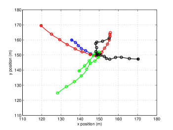
Figure 3: Scenario of simulations. There are four targets, all born at time step 1 and alive throughout the simulation, except the blue target that dies at time step 40, when all targets are in close proximity. Initial target positions have a cross and target positions every 5 time steps have a circle.

We consider 81 time steps and the scenario in Figure 3. These trajectories were generated as indicated in [18, Sec. VI]. For each trajectory, we initiate the midpoint (state at time step 41) from a Gaussian with mean $\left[150,0,150,0\right]^{T}$ and covariance matrix $0.1I_{4}$ and the rest of the trajectory is generated running forward and backward dynamics. This scenario is challenging due to the broad Poisson prior that covers the region of interest, the high number of targets in close proximity and the fact that one target dies when they are in close proximity. We perform 100 Monte Carlo runs and obtain the root mean square optimal subpattern assignment (OSPA) error $\left(p=2,\,c=10\right)$ [33, 40] at each time step for each algorithm, as shown in Figure 4. Estimator 1 applied to the PMBM filter provides the lowest errors followed by Estimators 2 and 3, which behave similarly. MOMB performs as accurately as Estimators 2 and 3 of the PMBM. It takes TOMB a long time to determine that one target disappears at time step 40. PHD and CPHD are rougher approximations and do not perform well in this scenario.

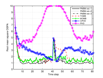
Figure 4: Mean OSPA error for the algorithms for $p_{d}=0.9$ and . The PMBM filter outperforms the rest of the algorithms. Estimator 1 of the PMBM filter provides lowest error and Estimators 2 and 3 perform similarly.

We also show the root mean square OSPA error averaged over all time steps of the algorithms for different values of $p_{d}$ and $\lambda_{c}=10$ in Table II. On the whole, the PMBM filter performs better than the rest regardless of the estimator. Estimator 1 has lower error than Estimator 2 and 3 for $p_{d}$ equal or higher than 0.9. For lower values of $p_{d}$, Estimator 2 provides lowest errors. The MOMB has the second best performance followed by the TOMB algorithm. The CPHD and PHD filters perform much worse than the other filters.

Table II: Root mean square OSPA error for the algorithms at all time steps

$\left(p_{d},\lambda_{c}\right)$	PMBM Est 1	PMBM Est 2	PMBM Est 3	TOMB	MOMB	CPHD	PHD
$\left(0.95,10\right)$	2.10	2.10	2.10	2.32	2.10	2.83	6.34
$\left(0.95,15\right)$	2.15	2.17	2.15	2.48	2.17	2.97	6.44
$\left(0.95,20\right)$	2.26	2.27	2.26	2.61	2.27	3.00	6.51
$\left(0.9,10\right)$	2.23	2.34	2.36	2.65	2.37	3.39	7.05
$\left(0.9,15\right)$	2.30	2.42	2.44	2.75	2.45	3.45	7.04
$\left(0.9,20\right)$	2.37	2.48	2.50	2.80	2.53	2.57	7.18
$\left(0.8,10\right)$	2.67	2.64	2.66	2.95	2.78	4.19	8.22
$\left(0.8,15\right)$	2.80	2.78	2.80	3.15	2.88	4.25	8.23
$\left(0.8,20\right)$	2.93	2.90	2.92	3.18	3.00	4.48	8.34
$\left(0.7,10\right)$	3.02	2.99	3.01	3.47	3.15	4.83	8.80
$\left(0.7,15\right)$	3.10	3.07	3.09	3.57	3.24	4.99	8.86
$\left(0.7,20\right)$	3.29	3.25	3.28	3.67	3.41	5.09	8.87
$\left(0.6,10\right)$	3.42	3.39	3.42	3.81	3.55	5.30	9.09
$\left(0.6,15\right)$	3.62	3.60	3.62	4.03	3.72	5.52	9.14
$\left(0.6,20\right)$	3.71	3.69	3.71	4.09	3.82	5.61	9.18

VIII Conclusions

In this paper, we have first provided a non-PGFL derivation of the Poisson multi-Bernoulli mixture filter in [18], showing its conjugacy property. In order to attain this, we have used a suitable representation of the prior density, which is the union of a Poisson and a multi-Bernoulli mixture, as well as different representations of the likelihood function at several steps. In addition, we have also proved that this derivation can be directly extended to the labelled case by removing the Poisson component and adding unique labels to the Bernoulli components. We have also explained that the PMBM filter parameterisation has important benefits compared to the $\delta$-GLMB filter parameterisation, which considers hypotheses with deterministic cardinality.

We have also provided an implementation of the Poisson multi-Bernoulli mixture filter for linear/Gaussian measurement models and Poisson births and clutter. The multi-Bernoulli mixture is a more efficient parameterisation of the filtering density than the $\delta$-GLMB form and, consequently, the prediction step is greatly simplified. Based on the multiple target tracking literature on MHT and labelled random finite sets, we have suggested three suboptimal estimators for the PMBM filter and how they can be obtained efficiently. Finally, we have compared the performance of the PMBM filter with other RFS filters in a challenging scenario, in which new born targets are distributed according to a Poisson RFS with an intensity that covers the surveillance area and several targets get in close proximity. PMBM outperforms the rest of the filters in this scenario.

Appendix A

In this appendix, we prove (13). We denote

$$l_{s}\left(\left\{z_{1},...,z_{m}\right\}|X\right) =e^{-\lambda_{c}}\sum_{U\uplus Y_{1}...\uplus Y_{m}=X}\left[1-p_{d}\left(\cdot\right)\right]^{U}$$

$$\quad\times\prod_{i=1}^{m}\tilde{l}\left(z_{i}|Y_{i}\right).$$ (52)

We perform a proof by induction. In the rest of this appendix, we denote $Z=\left\{z_{1},...,z_{m}\right\}$ and $X=\left\{x_{1},...,x_{n}\right\}$ for notational simplicity. First, we note that

$$l\left(\emptyset|\emptyset\right) =l_{s}\left(\emptyset|\emptyset\right)=e^{-\lambda_{c}}.$$ (53)

The result is proved if we prove that

$$l\left(\left\{z_{1},...,z_{j}\right\}|\left\{x_{1},...,x_{i}\right\}\right) =l_{s}\left(\left\{z_{1},...,z_{j}\right\}|\left\{x_{1},...,x_{i}\right\}\right)$$ (54)

for $j\leq m$ and $i\leq n$, implies that

$$l\left(Z\uplus\left\{z_{m+1}\right\}|X\right) =l_{s}\left(Z\uplus\left\{z_{m+1}\right\}|X\right)$$ (55)

and

$$l\left(Z|X\uplus\left\{x_{n+1}\right\}\right) =l_{s}\left(Z|X\uplus\left\{x_{n+1}\right\}\right).$$ (56)

A-A First part

We proceed to prove (55). We have that

$$l_{s}\left(Z\uplus\left\{z_{m+1}\right\}|X\right)$$

$$=e^{-\lambda_{c}}\sum_{U\uplus Y_{1}...\uplus Y_{m}\uplus Y_{m+1}=X}\left[1-p_{d}\left(\cdot\right)\right]^{U}\prod_{i=1}^{m+1}\tilde{l}\left(z_{i}|Y_{i}\right)$$

$$=e^{-\lambda_{c}}\sum_{Y_{m+1}\subseteq X}\tilde{l}\left(z_{m+1}|Y_{m+1}\right)\sum_{U\uplus Y_{1}\uplus...\uplus Y_{m}=X\setminus Y_{m+1}}$$

$$\;\times\left[1-p_{d}\left(\cdot\right)\right]^{U}\prod_{i=1}^{m}\tilde{l}\left(z_{i}|Y_{i}\right)$$

$$=\sum_{Y_{m+1}\subseteq X}\tilde{l}\left(z_{m+1}|Y_{m+1}\right)l_{s}\left(Z|X\setminus Y_{m+1}\right)$$

$$=\tilde{l}\left(z_{m+1}|\emptyset\right)l_{s}\left(Z|X\right)+\sum_{j=1}^{n}\tilde{l}\left(z_{m+1}|\left\{x_{j}\right\}\right)l_{s}\left(Z|X\setminus\left\{x_{j}\right\}\right).$$ (57)

We also have

$$l\left(Z\uplus\left\{z_{m+1}\right\}|X\right)$$

$$=e^{-\lambda_{c}}\sum_{Z^{c}\uplus Z_{1}...\uplus Z_{n}=Z\uplus\left\{z_{m+1}\right\}}\left[c\left(\cdot\right)\right]^{Z^{c}}\prod_{i=1}^{n}\hat{l}\left(Z_{i}|x_{i}\right)$$

$$=e^{-\lambda_{c}}\left[\sum_{Z^{c}\uplus Z_{1}...\uplus Z_{n}=Z\uplus\left\{z_{m+1}\right\}:z_{m+1}\in Z^{c}}\left[c\left(\cdot\right)\right]^{Z^{c}}\prod_{i=1}^{n}\hat{l}\left(Z_{i}|x_{i}\right)\right.$$

$$\;\left.+\sum_{j=1}^{n}\sum_{Z^{c}\uplus Z_{1}...\uplus Z_{n}=Z\uplus\left\{z_{m+1}\right\}:z_{m+1}\in Z_{j}}\left[c\left(\cdot\right)\right]^{Z^{c}}\prod_{i=1}^{n}\hat{l}\left(Z_{i}|x_{i}\right)\right]$$

$$=e^{-\lambda_{c}}\left[\tilde{l}\left(z_{m+1}|\emptyset\right)\sum_{Z^{c}\uplus Z_{1}...\uplus Z_{n}=Z}\left[c\left(\cdot\right)\right]^{Z^{c}}\prod_{i=1}^{n}\hat{l}\left(Z_{i}|x_{i}\right)\right.$$

$$\;+\sum_{j=1}^{n}\hat{l}\left(\left\{z_{m+1}\right\}|x_{j}\right)\sum_{Z^{c}\uplus Z_{1}...\uplus Z_{n}=Z:Z_{j}=\emptyset}\left[c\left(\cdot\right)\right]^{Z^{c}}$$

$$\left.\;\times\prod_{i=1:i\neq j}^{n}\hat{l}\left(Z_{i}|x_{i}\right)\right]$$

$$=\tilde{l}\left(z_{m+1}|\emptyset\right)l\left(Z|X\right)+\sum_{i=1}^{n}\tilde{l}\left(z_{m+1}|\left\{x_{i}\right\}\right)l\left(Z|X\setminus\left\{x_{i}\right\}\right).$$ (58)

Using the induction hypothesis (54), (58) equals (57), so we finish the proof of (55).

A-B Second part

We proceed to prove (56). In this part, we denote $p_{d}^{\prime}\left(\cdot\right)=1-p_{d}\left(\cdot\right)$. We have that

$$l_{s}\left(Z|X\uplus\left\{x_{n+1}\right\}\right)$$

$$=e^{-\lambda_{c}}\sum_{U\uplus Y_{1}...\uplus Y_{m}=X\uplus\left\{x_{n+1}\right\}}\left[p_{d}^{\prime}\left(\cdot\right)\right]^{U}\prod_{i=1}^{m}\tilde{l}\left(z_{i}|Y_{i}\right)$$

$$=e^{-\lambda_{c}}\left[\sum_{U\uplus Y_{1}...\uplus Y_{m}=X\uplus\left\{x_{n+1}\right\}:x_{n+1}\in U}\left[p_{d}^{\prime}\left(\cdot\right)\right]^{U}\prod_{i=1}^{m}\tilde{l}\left(z_{i}|Y_{i}\right)\right.$$

$$\;\left.+\sum_{j=1}^{m}\sum_{U\uplus Y_{1}...\uplus Y_{m}=X\uplus\left\{x_{n+1}\right\}:x_{n+1}\in Y_{j}}\left[p_{d}^{\prime}\left(\cdot\right)\right]^{U}\prod_{i=1}^{m}\tilde{l}\left(z_{i}|Y_{i}\right)\right]$$

$$=e^{-\lambda_{c}}\left[p_{d}^{\prime}\left(x_{n+1}\right)\sum_{U\uplus Y_{1}...\uplus Y_{m}=X}\left[p_{d}^{\prime}\left(\cdot\right)\right]^{U}\prod_{i=1}^{m}\tilde{l}\left(z_{i}|Y_{i}\right)\right.$$

$$\;+\sum_{j=1}^{m}\tilde{l}\left(z_{j}|\left\{x_{n+1}\right\}\right)\sum_{U\uplus Y_{1}...\uplus Y_{m}=X:Y_{j}=\emptyset}\left[p_{d}^{\prime}\left(\cdot\right)\right]^{U}$$

$$\left.\;\times\prod_{i=1:i\neq j}^{n}\tilde{l}\left(z_{i}|Y_{i}\right)\right]$$

$$=p_{d}^{\prime}\left(x_{n+1}\right)l_{s}\left(Z|X\right)+\sum_{j=1}^{m}\tilde{l}\left(z_{j}|\left\{x_{n+1}\right\}\right)l_{s}\left(Z\setminus\left\{z_{j}\right\}|X\right).$$ (59)

We also have that

$$l\left(Z|X\uplus\left\{x_{n+1}\right\}\right)$$

$$=e^{-\lambda_{c}}\sum_{Z^{c}\uplus Z_{1}...\uplus Z_{n+1}=Z}\left[c\left(\cdot\right)\right]^{Z^{c}}\prod_{i=1}^{n+1}\hat{l}\left(Z_{i}|x_{i}\right)$$

$$=e^{-\lambda_{c}}\sum_{Z_{n+1}\subseteq Z}\hat{l}\left(Z_{n+1}|x_{n+1}\right)$$

$$\;\times\sum_{Z^{c}\uplus Z_{1}...\uplus Z_{n}=Z\setminus Z_{n+1}}\left[c\left(\cdot\right)\right]^{Z^{c}}\prod_{i=1}^{n}\hat{l}\left(Z_{i}|x_{i}\right)$$

$$=e^{-\lambda_{c}}\left[p_{d}^{\prime}\left(x_{n+1}\right)\sum_{Z^{c}\uplus Z_{1}...\uplus Z_{n}=Z}\left[c\left(\cdot\right)\right]^{Z^{c}}\prod_{i=1}^{n}\hat{l}\left(Z_{i}|x_{i}\right)\right.$$

$$\left.\;+\sum_{j=1}^{m}\tilde{l}\left(z_{j}|\left\{x_{n+1}\right\}\right)\sum_{Z^{c}\uplus Z_{1}...\uplus Z_{n}=Z\setminus\left\{z_{j}\right\}}\left[c\left(\cdot\right)\right]^{Z^{c}}\prod_{i=1}^{n}\hat{l}\left(Z_{i}|x_{i}\right)\right]$$

$$=p_{d}^{\prime}\left(x_{n+1}\right)l\left(Z|X\right)+\sum_{j=1}^{m}\tilde{l}\left(z_{j}|\left\{x_{n+1}\right\}\right)l\left(Z\setminus\left\{z_{j}\right\}|X\right).$$ (60)

Given that the induction hypothesis (54) holds, (59) and (60) are identical, so we finish the proof of (56).

Appendix B

In this appendix, we show how to update a Poisson prior, whose result is given in (16)-(24). Substituting (13) into (15), we find

$$q^{p}\left(X|Z\right)$$

$$\propto f^{p}\left(X\right)\sum_{U\uplus Y_{1}...\uplus Y_{m}=X}\left[1-p_{d}\left(\cdot\right)\right]^{U}\prod_{i=1}^{m}\tilde{l}\left(z_{i}|Y_{i}\right)$$

$$=\sum_{U\uplus Y_{1}...\uplus Y_{m}=X}\left[1-p_{d}\left(\cdot\right)\right]^{U}\left[\prod_{i=1}^{m}\tilde{l}\left(z_{i}|Y_{i}\right)\right]$$

$$\quad\times f^{p}\left(U\uplus Y_{1}...\uplus Y_{m}\right)$$

$$\propto\sum_{U\uplus Y_{1}...\uplus Y_{m}=X}\left[1-p_{d}\left(\cdot\right)\right]^{U}f^{p}\left(U\right)\left[\prod_{i=1}^{m}\tilde{l}\left(z_{i}|Y_{i}\right)f^{p}\left(Y_{i}\right)\right]$$

$$\propto\sum_{U\uplus Y_{1}\uplus...\uplus Y_{m}=X}q^{p}\left(U\right)\left[\prod_{i=1}^{m}\rho^{p}\left(z_{i}\right)q^{p}\left(Y_{i}|z_{i}\right)\right].$$

In the previous derivation, we have used that $f^{p}\left(U\uplus Y_{1}...\uplus Y_{m}\right)\propto f^{p}\left(U\right)\prod_{i=1}^{m}f^{p}\left(Y_{i}\right)$, see (8), and Equations (18) and (19). The specific form of $q^{p}\left(Y_{i}|z_{i}\right)$, which is given in (20), is obtained straightforwardly by calculating (19).

Appendix C

In this appendix, we prove (27). By definition, we know that (27) is met for $n=0$ as $l_{o}\left(Z|Y\right)=l\left(Z|Y\right)$. By induction, Equation (27) is proved if the equality

$$l_{o}\left(Z|Y,X_{1},...,X_{n}\right) =l\left(Z|Y\uplus X_{1}\uplus...\uplus X_{n}\right)$$

implies

$$l_{o}\left(Z|Y,X_{1},...,X_{n},X_{n+1}\right) =l\left(Z|Y\uplus X_{1}\uplus...\uplus X_{n}\uplus X_{n+1}\right).$$

We have to prove two cases: $X_{n+1}=\emptyset$ and $X_{n+1}=\left\{x\right\}$. For $X_{n+1}=\emptyset$, we have that $Z_{n+1}=\emptyset$ so that $t\left(Z_{n+1}|X_{n+1}\right)\neq 0$. Therefore,

$$l_{o}\left(Z|Y,X_{1},...,X_{n},\emptyset\right)$$

$$\quad=\sum_{Z_{1}\uplus...\uplus Z_{n}\uplus Z^{y}=Z}l\left(Z^{y}|Y\right)\prod_{i=1}^{n}t\left(Z_{i}|X_{i}\right)$$

$$\quad=l_{o}\left(Z|Y,X_{1},...,X_{n}\right)$$

$$\quad=l\left(Z|X\uplus\emptyset\right)$$

where $X=Y\uplus X_{1}\uplus...\uplus X_{n}$. This proves the first case.

For $X_{n+1}=\left\{x\right\}$, we have

$$l_{o}\left(Z|Y,X_{1},...,X_{n},\left\{x\right\}\right)$$

$$=\sum_{Z_{1}...\uplus Z_{n}\uplus Z_{n+1}\uplus Z^{y}=Z}l\left(Z^{y}|Y\right)t\left(Z_{i}|\left\{x\right\}\right)\prod_{i=1}^{n}t\left(Z_{i}|X_{i}\right)$$

$$=t\left(\emptyset|\left\{x\right\}\right)\sum_{Z_{1}...\uplus Z_{n}\uplus Z^{y}=Z}l\left(Z^{y}|Y\right)t\left(Z_{i}|\left\{x\right\}\right)\prod_{i=1}^{n}t\left(Z_{i}|X_{i}\right)$$

$$+\sum_{z\in Z}t\left(\left\{z\right\}|\left\{x\right\}\right)\sum_{Z_{1}\uplus...\uplus Z_{n}\uplus Z^{y}=Z\setminus\left\{z\right\}}l\left(Z^{y}|Y\right)t\left(Z_{i}|\left\{x\right\}\right)$$

$$\quad\times\prod_{i=1}^{n}t\left(Z_{i}|X_{i}\right)$$

$$=\left(1-p_{d}\left(x\right)\right)l\left(Z|X\right)$$

$$+p_{d}\left(x\right)\sum_{z\in Z}l\left(z|x\right)l\left(Z\setminus\left\{z\right\}|X\right)$$

$$=l\left(Z|X\uplus\left\{x\right\}\right)$$

where $X=Y\uplus X_{1}\uplus...\uplus X_{n}$. This proves the second case.

Appendix D

In this appendix, we prove the prediction step of Corollary 3. We consider that the new born targets follow an MBM with parameters

$$f_{b}^{mbm}\left(Y\right) \propto\sum_{j_{b}}\sum_{Y_{1}\uplus...\uplus Y_{n_{b}}=Y}\prod_{i_{b}=1}^{n_{b}}w_{j_{b},i_{b}}^{b}f_{j_{b},i_{b}}^{b}\left(Y_{i}\right).$$ (61)

As indicated in Section III-D, the predicted density of the survival targets when the Poisson intensity is zero is an MBM. We denote the parameters of this MBM as in (9). Then, the output of the prediction step is the multi-target density of the union of the survival targets and the new born targets, which can be computed using the convolution formula [9, Eq. (4.17)]

$$f_{pred}\left(W\right) =\sum_{X\uplus Y=W}f^{mbm}\left(X\right)f_{b}^{mbm}\left(Y\right)$$

$$\propto\sum_{X\uplus Y=W}\left[\sum_{j}\sum_{X_{1}\uplus...\uplus X_{n}=X}\prod_{i=1}^{n}w_{j,i}f_{j,i}\left(X_{i}\right)\right]$$

$$\quad\times\left[\sum_{j_{b}}\sum_{Y_{1}\uplus...\uplus Y_{n_{b}}=Y}\prod_{i_{b}=1}^{n_{b}}w_{j_{b},i_{b}}^{b}f_{j_{b},i_{b}}^{b}\left(Y_{i}\right)\right]$$

$$=\sum_{j}\sum_{j_{b}}\sum_{X_{1}\uplus...\uplus X_{n}\uplus Y_{1}\uplus...\uplus Y_{n_{b}}=W}$$

$$\quad\left[\prod_{i=1}^{n}w_{j,i}f_{j,i}\left(X_{i}\right)\right]\left[\prod_{i_{b}=1}^{n_{b}}w_{j_{b},i_{b}}^{b}f_{j_{b},i_{b}}^{b}\left(Y_{i}\right)\right]$$

which corresponds to an MBM.

Appendix E

In this appendix, we prove Proposition 7. We first prove how a labelled MBM, which contains the labelled MBM₀₁ as a particular case, can be written as a $\delta$-GLMB density. We write (39) as

$$f\left(X\right) =\sum_{j}w_{j}\sum_{X_{1}\uplus...\uplus X_{n}=X}\prod_{i=1}^{n}f_{j,i}^{lb}\left(X_{i}\right)$$ (62)

where we have normalised the weights of the global hypotheses such that $\sum_{j}w_{j}=1$ and $w_{j}\propto\prod_{i=1}^{n}w_{j,i}$. Let $\mathbb{L}=\left\{\ell_{1},...,\ell_{n}\right\}$ denote the set with all the possible target labels according to the density (39).

Both the $\delta$-GLMB density and the labelled multi-Bernoulli mixture are zero if 1) they are evaluated on a set that includes more than one target with the same label, or 2) if they are evaluated on a set that includes a target whose label does not belong to the label space $\mathbb{L}$. Therefore, the case of interest is when we evaluate the density with a set of targets with distinct labels that belong to $\mathbb{L}$. We evaluate the labelled multi-Bernoulli mixture (62) on a labelled set $\left\{\left(x_{1},\ell_{a_{1}}\right),...,\left(x_{p},\ell_{a_{p}}\right)\right\}$ where $\ell_{a_{1}},...,\ell_{a_{p}}$ are $p$ distinct labels that belong to $\mathbb{L}$. We also denote by $\ell_{a_{p+1}},...,\ell_{a_{n}}$ the rest of distinct labels in $\mathbb{L}$. As labels $\ell_{a_{1}},...,\ell_{a_{p}}$ are distinct, there is only one combination in the sum over $X_{1}\uplus...\uplus X_{n}=X$ that is non-zero. This yields

$$f\left(\left\{\left(x_{1},\ell_{a_{1}}\right),...,\left(x_{p},\ell_{a_{p}}\right)\right\}\right)$$

$$=\sum_{j}w_{j}\left[\prod_{m=1}^{p}r_{j,a_{m}}p_{j,a_{m}}\left(x_{m}\right)\right]\prod_{i=p+1}^{n}\left(1-r_{j,a_{i}}\right).$$ (63)

We proceed to write this density in the $\delta$-GLMB form [21]. We denote

$$w_{j}\left(\left\{\ell_{a_{1}},...,\ell_{a_{p}}\right\}\right) =w_{j}\left[\prod_{m=1}^{p}r_{j,a_{m}}\right]\prod_{i=p+1}^{n}\left(1-r_{j,a_{i}}\right).$$ (64)

In the $\delta$-GLMB filter, this weight is written as (see sentence that contains Eq. (9) in [21])

$$w_{j}\left(\left\{\ell_{a_{1}},...,\ell_{a_{p}}\right\}\right) =\sum_{I\subseteq\mathbb{L}}w_{j}\left(I\right)\delta_{I}\left(\left\{\ell_{a_{1}},...,\ell_{a_{p}}\right\}\right),$$ (65)

where [21]

$$\delta_{I}\left(L\right) \triangleq\begin{cases}1&\mathrm{if}\;I=L\\ 0&\mathrm{otherwise}\end{cases}$$

and it can be verified that $\sum_{j}\sum_{I\subseteq\mathbb{L}}w_{j}\left(I\right)=1$. The previous step is direct, as there is only one summand in (65) that is different from zero, which corresponds to (64). Following [21], we also denote $p_{\xi}\left(x,\ell\right)=p_{\xi,i\left(\ell\right)}\left(x\right)$ where $i\left(\ell\right)=i$ such that $\ell=\ell_{i}$ and index $j$ is denoted as $\xi$. Substituting this notation into (63), we find

$$f\left(\left\{\left(x_{1},\ell_{a_{1}}\right),...,\left(x_{p},\ell_{a_{p}}\right)\right\}\right)$$

$$=\sum_{\xi}\sum_{I\subseteq\mathbb{L}}w_{\xi}\left(I\right)\delta_{I}\left(\left\{\ell_{a_{1}},...,\ell_{a_{p}}\right\}\right)\prod_{m=1}^{p}p_{\xi}\left(x_{m},\ell_{a_{m}}\right),$$ (66)

which corresponds to the $\delta$-GLMB density [21, Eq. (9)] evaluated on a set of targets with different labels.

In order to finish the proof of Proposition 7, we write a $\delta$-GLMB density as a labelled MBM with MBM₀₁ parameterisation.

We consider that the label space is $\mathbb{L}=\left\{\ell_{1},...,\ell_{n}\right\}$, the $\delta$-GLMB single target densities are $p_{\xi}\left(\cdot,\ell_{i}\right)$ for all $\xi$ and $\ell_{i}\in\mathbb{L},$ and the global hypothesis weights are $w_{\xi}\left(I\right)$ for $I\subseteq\mathbb{L}$. In order to prove the equivalence, we evaluate a $\delta$-GLMB density $f\left(\cdot\right)$ at $\left\{\left(x_{1},\ell_{a_{1}}\right),...,\left(x_{p},\ell_{a_{p}}\right)\right\}$, which is given by (66), with $\left\{\ell_{a_{1}},...,\ell_{a_{p}}\right\}\subseteq\mathbb{L}$. We also denote by $\ell_{a_{p+1}},...,\ell_{a_{n}}$ the rest of distinct labels in $\mathbb{L}$. It should be noted that the pair $\left(\xi,I\right)$ represents a $\delta$-GLMB global hypothesis [21] and that, in this global hypothesis, all targets whose label belongs to $I$ exist and the rest do not exist, which is represented by $\delta_{I}\left(\left\{\ell_{a_{1}},...,\ell_{a_{p}}\right\}\right)$ in (66). For global hypothesis $\left(\xi,I\right)$, this factor can be written as a product of existence probabilities, which are either 0 or 1, as

$$\delta_{I}\left(\left\{\ell_{a_{1}},...,\ell_{a_{p}}\right\}\right)$$

$$\>=\left[\prod_{m=1}^{p}r_{\left(\xi,I\right),a_{m}}\right]\left[\prod_{i=p+1}^{n}\left(1-r_{\left(\xi,I\right),a_{i}}\right)\right],$$ (67)

where $r_{\left(\xi,I\right),a_{m}}=1$ if $\ell_{a_{m}}\in I$ and $r_{\left(\xi,I\right),a_{m}}=0$ if $\ell_{a_{m}}\notin I$ for $m\in\left\{1,...,n\right\}$. We can write the two sums in (66) as one sum over $j=\left(\xi,I\right)$ such that

$$f\left(\left\{\left(x_{1},\ell_{a_{1}}\right),...,\left(x_{p},\ell_{a_{p}}\right)\right\}\right)$$

$$=\sum_{j}w_{j}\left[\prod_{m=1}^{p}r_{j,a_{m}}\right]\left[\prod_{i=p+1}^{n}\left(1-r_{j,a_{i}}\right)\right]\prod_{m=1}^{p}p_{j,a_{m}}\left(x_{m}\right)$$ (68)

where $p_{\left(\xi,I\right),a_{m}}\left(\cdot\right)=p_{\xi}\left(\cdot,\ell_{a_{m}}\right)$, $w_{\left(\xi,I\right)}=w_{\xi}\left(I\right)$. It should be noted that, in the $\delta$-GLMB density, we have $\sum_{\xi}\sum_{I\subseteq\mathbb{L}}w_{\xi}\left(I\right)=1$, which implies that $\sum_{j}w_{j}=1$, as required. Also note that $r_{j,i}$ is the existence probability of Bernoulli component $i$, with label $\ell_{i}$, and global hypothesis $j$, which is either 0 or 1. Equation (68) corresponds to the evaluation of a labelled multi-Bernoulli mixture, see Equation (63). In particular, the resulting global hypotheses (mixture components) of the $\delta$-GLMB density are equivalent to the global hypotheses in an MBM₀₁ parameterisation, which have deterministic target existence.

References

• [1] S. S. Blackman, “Multiple hypothesis tracking for multiple target tracking,” IEEE Aerospace and Electronic Systems Magazine, vol. 19, no. 1, pp. 5–18, Jan. 2004.
• [2] W. Koch and F. Govaers, “On accumulated state densities with applications to out-of-sequence measurement processing,” IEEE Transactions on Aerospace and Electronic Systems, vol. 47, no. 4, pp. 2766–2778, 2011.
• [3] J. García, A. Berlanga, and J. M. M. López, “Effective evolutionary algorithms for many-specifications attainment: Application to air traffic control tracking filters,” IEEE Transactions on Evolutionary Computation, vol. 13, no. 1, pp. 151–168, Feb. 2009.
• [4] H. Bhaskar, K. Dwivedi, D. P. Dogra, M. Al-Mualla, and L. Mihaylova, “Autonomous detection and tracking under illumination changes, occlusions and moving camera,” Signal Processing, vol. 117, pp. 343–354, 2015.
• [5] A. Petrovskaya and S. Thrun, “Model based vehicle detection and tracking for autonomous urban driving,” Autonomous Robots, vol. 26, no. 2, pp. 123–139, 2009.
• [6] F. Kunz et al., “Autonomous driving at Ulm university: A modular, robust, and sensor-independent fusion approach,” in IEEE Intelligent Vehicles Symposium, June 2015, pp. 666–673.
• [7] C. Fantacci and F. Papi, “Scalable multisensor multitarget tracking using the marginalized $\delta$-GLMB density,” IEEE Signal Processing Letters, vol. 23, no. 6, pp. 863–867, June 2016.
• [8] F. Meyer, P. Braca, P. Willett, and F. Hlawatsch, “A scalable algorithm for tracking an unknown number of targets using multiple sensors,” IEEE Transactions on Signal Processing, vol. 65, no. 13, pp. 3478–3493, July 2017.
• [9] R. P. S. Mahler, Advances in Statistical Multisource-Multitarget Information Fusion.   Artech House, 2014.
• [10] X. Li and V. Jilkov, “Survey of maneuvering target tracking. Part I: Dynamic models,” IEEE Transactions on Aerospace and Electronic Systems, vol. 39, no. 4, pp. 1333–1364, Oct. 2003.
• [11] A. Swain and D. Clark, “Extended object filtering using spatial independent cluster processes,” in 13th Conference on Information Fusion, July 2010, pp. 1–8.
• [12] K. Granström, C. Lundquist, and O. Orguner, “Extended target tracking using a Gaussian-mixture PHD filter,” IEEE Transactions on Aerospace and Electronic Systems, vol. 48, no. 4, pp. 3268–3286, October 2012.
• [13] A. F. García-Fernández, J. Grajal, and M. R. Morelande, “Two-layer particle filter for multiple target detection and tracking,” IEEE Transactions on Aerospace and Electronic Systems, vol. 49, no. 3, pp. 1569–1588, July 2013.
• [14] S. J. Davey, M. G. Rutten, and B. Cheung, “A comparison of detection performance for several track-before-detect algorithms,” in EURASIP Journal on Advances in Signal Processing, vol. 2008, 2008, pp. 1–10.
• [15] B. Ristic, S. Arulampalam, and N. Gordon, Beyond the Kalman Filter: Particle Filters for Tracking Applications.   Artech House, 2004.
• [16] C. P. Robert, The Bayesian Choice.   Springer, 2007.
• [17] B. T. Vo and B. N. Vo, “Labeled random finite sets and multi-object conjugate priors,” IEEE Transactions on Signal Processing, vol. 61, no. 13, pp. 3460–3475, July 2013.
• [18] J. L. Williams, “Marginal multi-Bernoulli filters: RFS derivation of MHT, JIPDA and association-based MeMBer,” IEEE Transactions on Aerospace and Electronic Systems, vol. 51, no. 3, pp. 1664–1687, July 2015.
• [19] T. Kurien, “Issues in the design of practical multitarget tracking algorithms,” in Multitarget-Multisensor Tracking: Advanced Applications, Y. Bar-Shalom, Ed.   Artech House, 1990.
• [20] A. F. García-Fernández and J. Grajal, “Multitarget tracking using the joint multitrack probability density,” in 12th International Conference on Information Fusion, July 2009, pp. 595–602.
• [21] B.-N. Vo, B.-T. Vo, and D. Phung, “Labeled random finite sets and the Bayes multi-target tracking filter,” IEEE Transactions on Signal Processing, vol. 62, no. 24, pp. 6554–6567, Dec. 2014.
• [22] E. H. Aoki, P. K. Mandal, L. Svensson, Y. Boers, and A. Bagchi, “Labeling uncertainty in multitarget tracking,” IEEE Transactions on Aerospace and Electronic Systems, vol. 52, no. 3, pp. 1006–1020, June 2016.
• [23] R. Mahler, “PHD filters of higher order in target number,” IEEE Transactions on Aerospace and Electronic Systems, vol. 43, no. 4, pp. 1523–1543, October 2007.
• [24] R. P. S. Mahler, “Multitarget Bayes filtering via first-order multitarget moments,” IEEE Transactions on Aerospace and Electronic Systems, vol. 39, no. 4, pp. 1152–1178, Oct. 2003.
• [25] A. F. García-Fernández and B.-N. Vo, “Derivation of the PHD and CPHD filters based on direct Kullback-Leibler divergence minimization,” IEEE Transactions on Signal Processing, vol. 63, no. 21, pp. 5812–5820, Nov. 2015.
• [26] R. P. S. Mahler, Statistical Multisource-Multitarget Information Fusion.   Artech House, 2007.
• [27] J. L. Williams, “An efficient, variational approximation of the best fitting multi-Bernoulli filter,” IEEE Transactions on Signal Processing, vol. 63, no. 1, pp. 258–273, Jan. 2015.
• [28] S. Särkkä, Bayesian filtering and smoothing.   Cambridge University Press, 2013.
• [29] K. G. Murty, “An algorithm for ranking all the assignments in order of increasing cost.” Operations Research, vol. 16, no. 3, pp. 682–687, 1968.
• [30] I. J. Cox and M. L. Miller, “On finding ranked assignments with application to multitarget tracking and motion correspondence,” IEEE Transactions on Aerospace and Electronic Systems, vol. 31, no. 1, pp. 486–489, Jan 1995.
• [31] I. J. Cox and S. L. Hingorani, “An efficient implementation of Reid’s multiple hypothesis tracking algorithm and its evaluation for the purpose of visual tracking,” IEEE Transactions on Pattern Analysis and Machine Intelligence, vol. 18, no. 2, pp. 138–150, Feb 1996.
• [32] E. Fortunato, W. Kreamer, S. Mori, C.-Y. Chong, and G. Castanon, “Generalized Murty’s algorithm with application to multiple hypothesis tracking,” in International Conference on Information Fusion, July 2007.
• [33] D. Schuhmacher, B.-T. Vo, and B.-N. Vo, “A consistent metric for performance evaluation of multi-object filters,” IEEE Transactions on Signal Processing, vol. 56, no. 8, pp. 3447–3457, Aug. 2008.
• [34] M. Guerriero, L. Svensson, D. Svensson, and P. Willett, “Shooting two birds with two bullets: How to find minimum mean OSPA estimates,” in 13th Conference on Information Fusion, July 2010, pp. 1–8.
• [35] M. Fernandez and S. Williams, “Closed-form expression for the Poisson-binomial probability density function,” IEEE Transactions on Aerospace and Electronic Systems, vol. 46, no. 2, pp. 803–817, April 2010.
• [36] D. Reid, “An algorithm for tracking multiple targets,” IEEE Transactions on Automatic Control, vol. 24, no. 6, pp. 843–854, Dec. 1979.
• [37] S. Mori, C.-Y. Chong, E. Tse, and R. Wishner, “Tracking and classifying multiple targets without a priori identification,” IEEE Transactions on Automatic Control, vol. 31, no. 5, pp. 401–409, May 1986.
• [38] B.-N. Vo and W.-K. Ma, “The Gaussian mixture probability hypothesis density filter,” IEEE Transactions on Signal Processing, vol. 54, no. 11, pp. 4091–4104, Nov. 2006.
• [39] B.-T. Vo, B.-N. Vo, and A. Cantoni, “Analytic implementations of the cardinalized probability hypothesis density filter,” IEEE Transactions on Signal Processing, vol. 55, no. 7, pp. 3553–3567, July 2007.
• [40] A. S. Rahmathullah, A. F. García-Fernández, and L. Svensson, “Generalized optimal sub-pattern assignment metric,” in 20th International Conference on Information Fusion, 2017.