The Effect of Reactive Social Distancing on the 1918 Influenza Pandemic

Abstract

The 1918 influenza pandemic was characterized by multiple epidemic waves. We investigated into reactive social distancing, a form of behavioral responses, and its effect on the multiple influenza waves in the United Kingdom. Two forms of reactive social distancing have been used in previous studies: Power function, which is a function of the proportion of recent influenza mortality in a population, and Hill function, which is a function of the actual number of recent influenza mortality. Using a simple epidemic model with a Power function and one common set of parameters, we provided a good model fit for the observed multiple epidemic waves in London boroughs, Birmingham and Liverpool. Our approach is different from previous studies where separate models are fitted to each city. We then applied these model parameters obtained from fitting three cities to all 334 administrative units in England and Wales and including the population sizes of individual administrative units. We computed the Pearson’s correlation between the observed and simulated data for each administrative unit. We achieved a median correlation of 0.636, indicating our model predictions perform reasonably well. Our modelling approach which requires reduced number of parameters resulted in computational efficiency gain without over-fitting the model. Our works have both scientific and public health significance.

1 Introduction

The influenza pandemic of 1918 had been regarded as the deadliest pandemic in recorded history, as it had caused 50 million deaths worldwide [1]. Due to its exceptional lethality and unusual epidemiological features, an in-depth understanding of the 1918 pandemic can provide insights to future influenza pandemic control planning. The 1918 pandemic was characterized by multiple waves of mortality. In the United Kingdom, the pandemic took place as three distinct waves: the first wave in the summer of 1918, the second wave in autumn of the same year and the third wave in the spring of 1919. Earlier studies attempted to identify the underlying causes of multiple waves [2, 3, 4, 5]. They all pointed towards human behavioral responses being a key factor in the exhibition of multiple waves in the 1918 influenza pandemic. Human behavioral responses had been considered as a crucial factor that could influence the transmission of infectious diseases [6, 7, 8, 9, 10, 11, 12]. When an infectious disease invaded a population, people behaved reactively to reduce the probability of being infected, such as avoidance of mass gathering, putting on face masks and actively maintaining personal hygiene. He et al. showed that the temporal changes in transmission rates could be the most likely explanation for the three epidemic waves in England and Wales, and human behavioral changes had the largest effect on the epidemic waves of weekly cases [3, 4]. Poletti et al. studied the 2009 H1N1 influenza pandemic and concluded that human behavioral changes could have a significant impact on the timing, dynamics and magnitude of the epidemic spread [12]. Bootsma and Ferguson found that the effect of reactive social distancing could have a stronger impact on the epidemic waves of the weekly cases than on the overall mortality [2]. However, the impact of reactive social distancing on the final epidemic size remained unknown. In previous studies, an epidemic model with a common set of parameters for different cities did not fit the observed data well [2]. Here, we compare two mathematical functions of reactive social distancing: Power function, which is a function of the proportion of recent influenza mortality in a population, and Hill function, which is a function of the actual number of recent influenza mortality. This manuscript is arranged as follows: We fitted out model with the same set of input parameters to the observed data in London boroughs, Birmingham and Liverpool. We applied these model parameter values obtained from fitting three cities to all 334 administrative units in England and Wales and including the population sizes of individual administrative units. We demonstrated the impact of reactive social distancing on the final epidemic size. In the appendix, we showed the theoretical results of the oscillations induced by reactive social distancing.

2 Methods

2.1 Data

We analyzed data on weekly influenza deaths (either influenza was recorded as contributing or death has been assigned to influenza) between June 29, 1918 and May 10, 1919 from 334 Administrative units in England for London boroughs, Birmingham and Liverpool based on the publicly available data [13]. We obtained the daily temperatures from the UK Met Office (http://www.metoffice.gov.uk).

2.2 Model

Figure 1: Schematic diagram shows the transmission dynamics during a disease outbreak. $S$ denotes the number of susceptible individuals, $I$ denotes the number of infectious individuals, $R$ denotes the number of recovered individuals, $D$ denotes the number of individuals who are no longer infectious and are progressing to death of influenza or pneumonia causes, $M$ denotes the cumulative number of influenza-related deaths, and $W$ denotes recent influenza mortality.

Bootsma and Ferguson [2] proposed that people reduce their exposure to potentially infectious contacts in response to high mortality rates during an influenza pandemic. In this study, we assumed the perceived risk of influenza is proportional to the number of recent deaths, and that people practised social distancing in response to this perceived risk. Here, we employed a simple Susceptible-Infectious-Recovered (SIR) model to account for such behavioral changes in the population [4]. Our earlier study shows that similar results are achieved if an additional “exposed” class is included [4]. The model is represented as follows:

$$\begin{split}&\dot{S}=-\frac{\beta(t)}{N}SI,\\ &\dot{I}=\frac{\beta(t)}{N}SI-\gamma I,\\ &\dot{R}=\gamma(1-\phi)I,\\ &\dot{D}=\gamma\phi I-gD,\\ &\dot{M}=gD,\\ &\dot{W}=gD-\lambda W.\end{split}$$ (1)

Here, $S$ denotes the number of susceptible individuals, $I$ denotes the number of infectious individuals, $R$ denotes the number of individuals who are immune to the disease. $D$ denotes the number of individuals who are no longer infectious and are progressing to deaths of influenza or pneumonia causes. $M$ denotes the number of influenza deaths. $W$ denotes the recent influenza mortality, and we assume that the general public’s risk perception is based on W. $N$ is the population size which is assumed to be constant. The population sizes for London Borough, Birmingham and Liverpool were approximately 4,484,523, 919,444 and 802,940 during the study period, respectively. Parameter $\phi$ stands for case-fatality-ratio (CFR).

Parameters $\gamma$, $g$ and $\lambda$ are rates at which individuals move from one class to the next class. $\gamma^{-1}$ and $g^{-1}$ are the mean infectious period (to be fixed at 4 days [14]) and the mean time from loss-of-infectiousness to death (to be fixed at 8 days). Thus the mean duration from infection to death is 12 days [2]. $\lambda^{-1}$ is the duration of human risk-reduction behavior in days. Following [4], $\beta(t)$ is the transmission rate and takes the following form:

$$\begin{split}\beta(t)&=\beta_{0}\cdot e^{-\xi T(t)}\cdot[1+\alpha H(t)]\cdot\left[1-\frac{W(t)}{N}\right]^{\kappa}\end{split}$$ (2)

where there are four components

(i) $\beta_{0}$ is the constant baseline transmission rate.

(ii) $e^{-\xi T(t)}$ is the term representing the temperature effect, $T(t)$ is time series of daily temperature (the model is simulated with a step size of 1 day), the parameter $\xi$ controls the intensity of the temperature effect.

(iii) $1+\alpha H(t)$ is the factor of school terms with amplitude parameter $\alpha$ and school day function $H(t)$ (a step function takes a large value on school days and a small value otherwise, see [4]); Easter and Christmas holiday dates are known. However, the summer vacation period ($t_{1}$, $t_{2}$) is unknown, therefore the start date ($t_{1}$) and end date ($t_{2}$) are to be estimated. During the 1910’s, a large number of people, including both adults and school children, are involved in summer harvesting. Thus there is a substantial impact on influenza transmission. This was discussed in [4]).

(iv) The last factor is the human behavioral term, where $W(t)$ denotes the recent influenza mortality, and $\kappa$ represents the intensity of human behavioral response in relation to the risk of influenza infection.

Finally, we define the basic reproductive number $\mathcal{R}_{0}=\frac{\left\langle\beta(t)\right\rangle}{\gamma}$ with $W(t)=0$ (see [4], we have $W=0$ at disease-free equilibrium). Note that $\left\langle\beta(t)\right\rangle<\beta_{0}$, since the temperature effect has an average value of smaller than 1. However, with human behavioral reaction, it is more effective to estimate the effective reproductive number, $\mathcal{R}_{\text{eff}}(t)$ instead, which is defined as the actual average number of secondary cases per primary case of infection at time $t$ [15]. We have $\mathcal{R}_{\text{eff}}(t)=\beta(t)S(t)/(\gamma N)$[16]. If $\mathcal{R}_{\text{eff}}(t)\leq 1$, it indicates that the epidemic is under control.

Here, we use the formula $[1-\frac{W(t)}{N}]^{\kappa}$ to represent the effect of reactive social distancing on transmission rate. Bootsma and Ferguson [2] modelled the reactive social distancing as a Hill function $\frac{\kappa}{\kappa+W(t)}$. If we compare the Taylor’s series expansion in the Power function and the Hill function, we noted that $N/\kappa$ in the Hill function is equivalent to the $\kappa$ in the Power function. Furthermore, if we replace $\kappa$ with $N/\kappa$ in the Hill function, we will obtain a modified-Hill function. The first two terms in the Taylor’s series expansion in both the Power function and the modified-Hill function are almost the same.

Power $$\left[1-\frac{W(t)}{N}\right]^{\kappa} =1-\frac{\kappa}{N}W(t)+\frac{1}{2}\frac{\kappa(\kappa-1)}{N^{2}}W(t)^{2}+\cdots$$ (3a)

Hill $$\frac{\kappa}{\kappa+W(t)} =1-\frac{1}{\kappa}W(t)+\frac{1}{\kappa^{2}}W(t)^{2}+\cdots$$ (3b)

Modified Hill $$\frac{N/\kappa}{N/\kappa+W(t)} =1-\frac{\kappa}{N}W(t)+\frac{\kappa^{2}}{N^{2}}W(t)^{2}+\cdots$$ (3c)

The above suggests that the Power function and the modified-Hill function will lead to almost the same results. The key point is whether $W(t)$ is scaled by $N$ or not in the behavioral term.

2.3 Model Fitting and Parameter estimates

We fit the model as described in Figure  1 to the reported weekly influenza deaths from the three largest administrative units: London boroughs, Birmingham and Liverpool during the 1918-1919 influenza pandemic. We assumed the epidemiological parameters remained the same for all three cities, and then further modelled for all 334 administrative units in England and Wales by incorporating their respective population sizes $N$. Previous studies [2, 4] assumed that key parameter values being distinct for different cities or administrative units. Thus we greatly reduce the number of free parameters and computational time in this work. Our assumption is also biologically plausible as previous studies showed that the transmissibility during the pandemic showed little spatial variations [17, 18].

Partially observed Markov process (POMP) model within a plug-and-play framework [19] was applied to simulate the epidemic dynamics in equation 1. Parameters including baseline transmission rate ($\beta_{0}$), case-fatality-ratio ($\phi$), school-term impact intensity ($\alpha$), air temperature impact intensity ($\xi$), reactive social distancing intensity ($\kappa$) and rate of recovery of social distancing ($\lambda$) are estimated by the Iterated Filtering method, allowing us to compute the maximum likelihood [20, 21].

Using this method, stochastic perturbation is added to the unknown parameters for the exploration of parameter space. This allows us to extend the range of global search, to avoid local minima and to construct an approximation to derive the log-likelihood. Selection of the estimates is achieved by Sequential Monte Carlo(SMC) or particle filtering, which keeps the results to be consistent with the data. With well-constructed procedures and continually decreasing perturbations, the iterations will converge to the maximum likelihood estimates. This method has been widely used in infectious disease modelling studies, including Ebola, cholera, malaria, influenza, as well as studies in finance and ecological dynamics. The ’pomp’ package in R is used for implementation (http://kingaa.github.io/pomp/).

3 Results

Figure 2 shows the best-fitting simulation models using three different functions, i.e. a model with the Power function (panels a-c), the Hill function (panels d-f) and the modified-Hill function (panels h-j). The inset panels show the log-likelihood profile of each model as a function of the parameter $\kappa$. Since the numbers of parameters of the three models (i.e. their model complexity) are the same, we can directly compare their Maximum Log Likelihoods (MLL). The MLLs for the Power function, the Hill function and the modified-Hill function are -596.12, -659.58 and -596.34 respectively. Since a larger MLL indicates a better model fit, we conclude that both the Power function and the modified-Hill function provide the best model choice. Thus, we identify a unified model (with the Power function or the modified-Hill function) for the three waves in these three cities. The Power function and the modified-Hill function virtually achieve the same goodness-of-fit levels, and both are superior to the Hill function used in [2], using our current dataset.

In previous studies [2, 4], key parameters such as $\mathcal{R}_{0}$ and $\kappa$ are assumed to be different for each city in order to achieve the best model fit. Our model fit as shown in Figure 2(a-c) are reasonably well, which use a unified model that estimated the same set of epidemiological parameters (i.e., the same $\kappa$ in all three cities), but using different population sizes and initial conditions for each of the three cities.

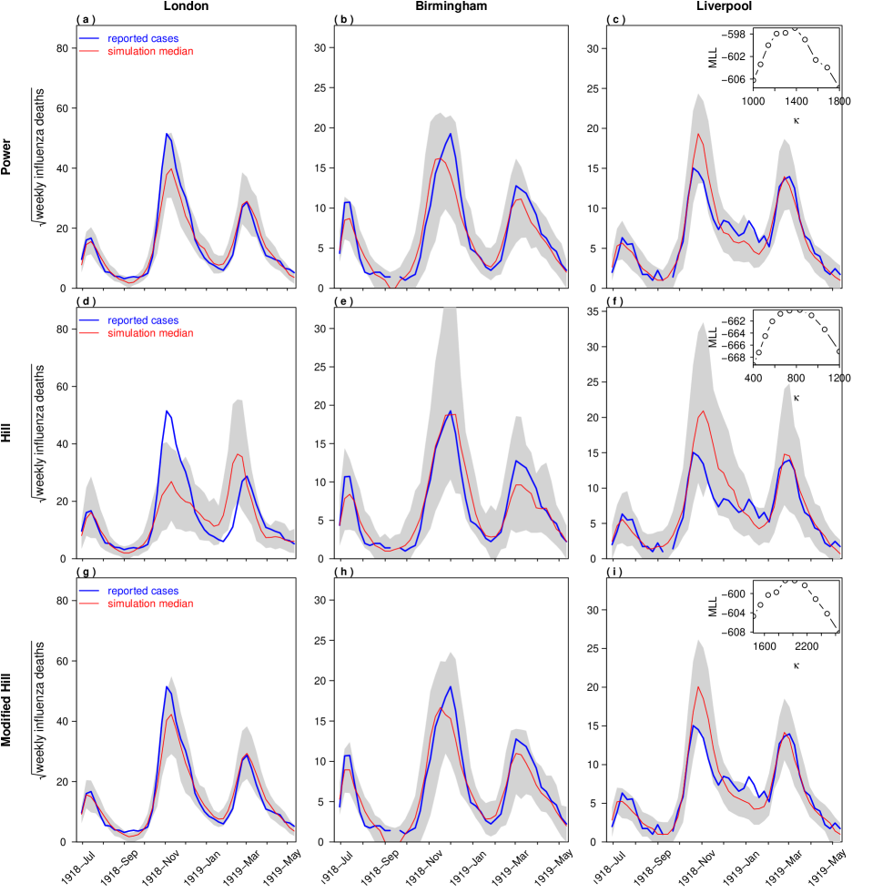
Figure 2: Simulation comparisons of the weekly influenza deaths during the 1918 pandemic in London, Birmingham and Liverpool. We used human behavioral terms of the (a-c) Power function, (d-f) Hill function, and (g-i) modified-Hill function. Blue bold line depicts the reported cases. Red thin line depicts the simulation median. The shaded area indicates the 95% confidence interval. The inset panels show the profile log-likelihood as a function of $\kappa$.

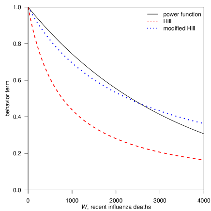
Figure 3: Comparison among the value of three behavioral functions with their best-fitted $\kappa$.

Figure 3 compares the three behavioral functions with the maximum likelihood estimates of $\kappa$. We can see that the Power function and the modified-Hill function largely overlaps, while the Hill function is clearly different from the other two functions.

Figure 4 shows the estimated daily reproductive number $\mathcal{R}_{0}$ (red thin curve) and the effective reproductive number $\mathcal{R}_{\text{eff}}$ (blue bold curve). The estimated daily reproductive number is identical in the three cities, since we assume all related parameters to be identical. The fluctuations in the daily reproductive number are due to school term and daily temperature, whereas we set $W=0$ (see [4]). In the effective reproductive number, we use the estimated $W(t)$ and susceptible $S(t)$. Thus $\mathcal{R}_{\text{eff}}$ is distinct among the cities and when it is greater than 1 (or less than 1), the mortality curve increases (or decreases) with a time delay of about 12 days.

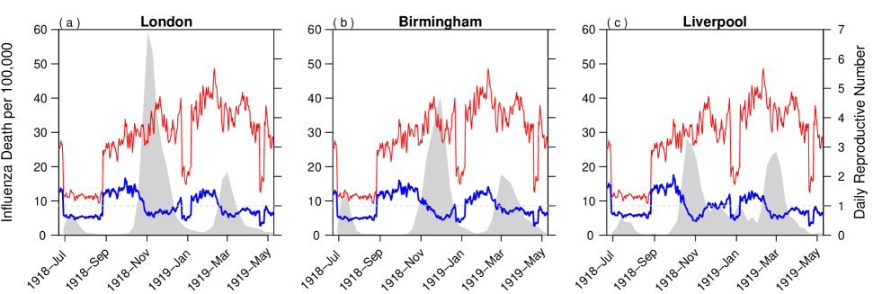
Figure 4: Estimated daily basic reproductive number $\mathcal{R}_{0}$ (red thin curve), effective reproductive number $\mathcal{R}_{\text{eff}}$ (blue bold curve) and weekly influenza deaths (shaded region). The average basic reproductive number is 3.24 in the three cities.

Table 1 summarizes all parameters used in the model with the Power function. All parameters values are largely biologically reasonable [2, 4]. Thus, we successfully find a model with common parameter values for all three cities. The only differences are in the population sizes and the initial conditions. We denote the initial susceptible population and initial population size to be $S_{0}$ and $I_{0}$, respectively. Note that the estimated initial conditions are similar among the three cities.

Table 1: Summary of all parameters estimated in the best-fitted model with a Power function.

Parameter	London boroughs	Birmingham	Liverpool	Type
initial, $S_{0}/N$	0.685 (0.503, 0.836)	0.677 (0.450,0.806)	0.632 (0.253, 0.950)	distinct
initial, $I_{0}$	9552 (7116, 14611)	3760 (2302, 4964)	927 (610, 1521)	distinct
behavioral, $\kappa$	1323.2 (1185.9, 1484.8)			common
delay, $\lambda^{-1}$ (days)	12.43 (10.73, 14.55)			common
CFR, $\phi$	0.0118 (0.0108, 0.0129)			common
baseline, $\beta_{0}$	4153.8 (3067.9, 8424.1			common
school-term, $\alpha$	0.437 (0.377, 0.498)			common
temperature, $\xi$	0.04048 (0.03441, 0.04568)			common
summer vacation start	June 23 (May 24, June 28)			common
summer vacation end	August 21 (Aug 12, August 31)			common

3.1 Applying the model to 334 administrative units

We apply our model with parameter values from fitting the three largest cities to all 334 administrative units in England and Wales. The only parameter we need to incorporate into this model is the population size of each administrative unit. As the three cities had similar initial conditions, we use that of Liverpool’s. We display our results in Figure 5. We compute the Pearson’s correlations between the observed (panel (a)) and simulated values (panel (b), with all three factors) for each administrative unit. The median correlation is 0.636. This shows that our model performs reasonably well in at least half of the 334 administrative units while only using data from three major cities. If the effects of behavioral changes are removed, previous studies [2, 4] show that the model cannot fit the data well even when the cities are being fitted separately. In panel (c), we show the simulation results of the 334 administrative units by setting $W=0$ and using other parameters from panel (b). It can been seen that model can only yield two wave, with the winter wave mmissed. Furthermore, we compare the overall attack rates in the two scenarios: Using all three factors, the estimated infection attack rate is about 28.5% (95% confidence interval: 14.1%, 35.9%). Without behavioral changes, the estimated infection attack rate is about 40.8% (95% CI: 34.0%, 46.9%). Thus the reduction due to behavioral changes is substantial.

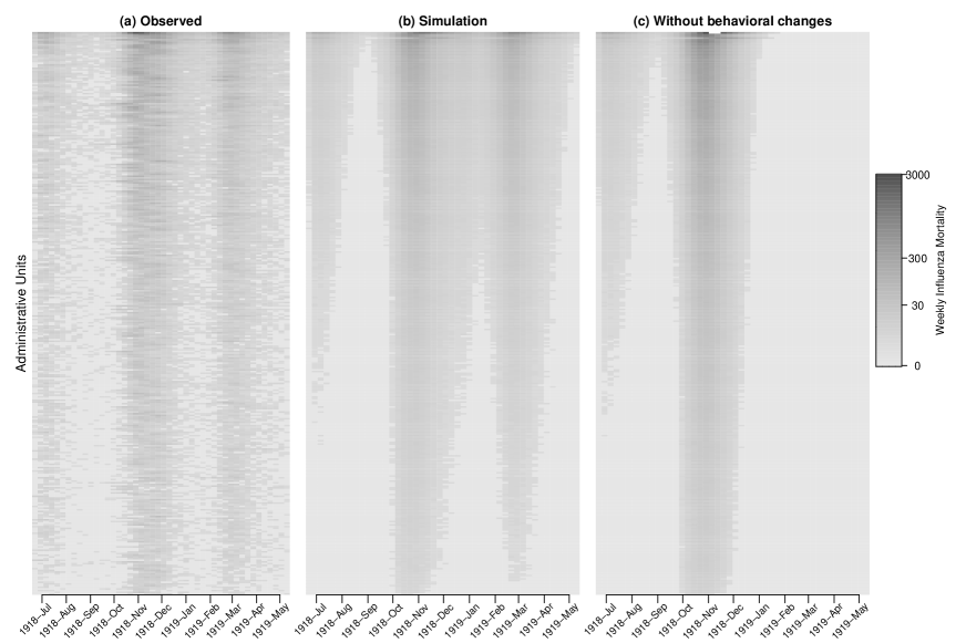
Figure 5: Comparison between the observed and simulated patterns of influenza deaths in 334 administrative units. (a) Observed. (b) Simulation with all three factors (school term, temperature, and behavioral changes). (c) Without behavioral changes. Administrative units are ordered in descending population sizes from top to bottom.

Discussion and Conclusions

Through a simple epidemic model with a Power function as behavioral term and a common set of parameters, we provided a good model fit for the observed multiple waves of influenza deaths in London boroughs, Birmingham and Liverpool. Our results are novel compared with earlier works by Bootsma and Ferguson [2] and He et al [4]. We also showed that the same set of parameters can be used for modelling the 334 administrative units. Furthermore, through given parameter values of mean infectious period and mean time from loss-of-infectiousness-to-death, we showed that there is an almost perfect linear relationship between the mean period of damping oscillation and the duration of reactive social distancing. Our theoretical damping oscillation results provided a plausible explanation to the observed multiple waves, where by reactively responding to the high proportion of influenza deaths with social distancing, the epidemic waves will be dampened. However, with the decline in the proportion of influenza deaths, public risk perception will be lowered as well, and the reduced social distancing could induce another epidemic wave. We also showed that reactive social distancing leads to a reduction in final epidemic size.

Our findings are plausible and are consistent with earlier mathematical modelling studies on the 1918 influenza pandemic [14, 22]. Bootsma and Ferguson [2] developed an epidemic model to study the impacts of public health interventions on the 1918 influenza pandemic in 16 U.S. cities. He et al [4] proposed another epidemic model which incorporates school opening and closing, temperature changes and changes in human behavioral response during the 1918 influenza pandemic in 334 administrative units of England and Wales. However, in both of these studies, instead of using a common set of model input parameters, unique model input parameters were needed for model fitting of each city or administrative units. Here, our model requires only a common set of parameters for the three-city or the subsequent 334-administrative model-fitting procedure, and the reduced number of model input parameters used represented significant improvement in computational efficiency and resulted in more robust estimates. Caley et al [5] studied the 1918 influenza pandemic in Australia, showing that reactive social distancing had a significant impact on the observed multiple epidemic waves and final epidemic size. Our effective reproductive numbers are comparable to these studies.

Compared to previous studies, our methods provide several improvements. Our study has the following strengths. First, by using a common set of model parameters for fitting the three-city model, we have greatly enhanced our computational efficiencies and have also resulted in more robust estimates of the final epidemic size. Second, we have identified an almost perfect linear relationship between the mean period of damping oscillations and duration of reactive social distancing on various combinations of mean infectious period and mean time from loss-of-infectiousness-to-death, which will be useful for future studies on the time between influenza epidemic waves. Major limitations of our study include the lack of direct historical behavioral data on quantifying the extent of reactive social distancing. Also, other non-pharmaceutical interventions could have played a role on the influenza pandemic patterns observed, but these measures are not considered in our model. There could be differences in summer vacation periods and daily temperature data in the three cities. However, such detailed data are not accessible to us. We could only make a simplifying assumption that they are the same across all locations. In future epidemics or pandemics, such information will be available and could be incorporated into the framework developed in this work.

In conclusion, a simple model with reactive social distancing, weather conditions, and school term could explain the observed multiple waves and final epidemic size in London boroughs, Birmingham and Liverpool during the 1918 influenza pandemic. Despite societal changes, our historical analyses on the 1918 pandemic could still serve as an important reference for future pandemic planning.

References

- [1] N.P. Johnson and J. Mueller. Bull. Hist. Med. 76, 105 (2002).
- [2] M.C. Bootsma and N.M. Ferguson. Proc Natl Acad Sci U S A. 104, 7588 (2007).
- [3] D. He et al. Theor. Ecol. 4, 283 (2011).
- [4] D. He et al. Proc Biol Sci. 280, 20131345 (2013).
- [5] P. Caley, D.J. Philp and K. McCracken. J R Soc Interface. 23, 631 (2008).
- [6] N. Ferguson. Nature. 446, 733 (2007).
- [7] S. Funk, M. Salathe and V.A. Jansen. 7, 1247 (2010).
- [8] S. Del Valle et al. Math Biosci. 195, 228 (2005).
- [9] J.M. Epstein et al. PLoS One. 3, e3955 (2008).
- [10] S. Funk, et al. Proc Natl Acad Sci U S A. 106, 6872 (2009).
- [11] T.C. Reluga. PLoS Comput Biol. 6, e1000793 (2010).
- [12] P. Poletti, et al. J Theor Biol. 260, 31 (2009).
- [13] N. Johnson. UK Data Service. SN: 4350, (2011).
- [14] C.E. Mills, J.M. Robins and M. Lipsitch. Nature. 432, 904 (2004).
- [15] H. Nishiura and G. Chowell. Euro Surveill. 19, 20894 (2014).
- [16] G. Chowell, et al. J Theor Biol. 229, 119 (2004).
- [17] G. Chowell et al. Proc. R. Soc. B. 275, 501 (2008).
- [18] R.M. Eggo, S. Cauchemez and N.M. Ferguson. J. R. Soc. Interface 8, 233 (2011).
- [19] D. He, E.L. Ionides and A.A. King. J R Soc Interface. 7, 271 (2010).
- [20] E.L. King, C. Breto and A.A. King. Proc Natl Acad Sci U S A. 103, 18438 (2006).
- [21] E. Ionides, et al. Ann Stat. 39, 1776 (2011).
- [22] N. M. Ferguson, D. Cummings, et al. Nature. 437, 7056 (2005).
Acknowledgment
We were supported by General Research Fund (Early Career Scheme) from Hong Kong Research Grants Council (PolyU 251001/14M) and Start-up Fund for New Recruits from Hong Kong Polytechnic University.