DRAFT: Numerical Integration and Dynamic Discretization in Heuristic Search Planning over Hybrid Domains

I.   Introduction

A central research topic in domain–independent automated planning is that of seeking plans over hybrid domain descriptions that feature both discrete and numeric state variables, as well as discrete instantaneous and continuous durative change via actions and processes Fox  Long (2006). A purely continuous dynamical system is defined by a set differential equations (ode’s) that specifies how the system evolves over time Scheinerman (2001). Hybrid planning problems correspond to control of switched dynamical systems, which are driven by different dynamics (set of ode’s) in different modes. A mode can be defined by the values of discrete state variables, a region of the continuous state space, or a combination of both Goebel . (2009); Ogata (2010). Planning languages, such as pddl$+$ and our extension of FSTRIPS, model switched dynamical systems compactly in a factored way, avoiding the explicit enumeration of modes.

This paper introduces a heuristic search hybrid planner, FS+. Like McDermott’s 2003 hybrid planner, OpTop, ours branches over the set of applicable instantaneous actions plus a special “waiting” action $sim$, that simulates continuous state evolution with the passing of time. The duration of the waiting action, that discretises time, is not fixed to a single value or a suitably chosen set like in Fox . (2012), but rather FS+ decides to use a smaller one than the initially set planning time step, $\Delta_{max}$. The successor state that results from applying the waiting action is the result of simulating system evolution, according to the dynamics of its current mode, for the duration of the step; computing it is known as the initial value problem in control theory Ogata (2010). For general dynamics there is no analytical solution to this problem, but approximate solutions can be obtained with a variety of numerical integration methods Butcher (2008). Such methods apply a finer discretisation, using a simulation time step $\Delta z$. Finally, a validation step verifies that the invariant condition of the mode  Howey  Long (2003) remains true throughout each simulation step. If it does not – which we refer to as a zero crossing event, following Shin & Davies 2005 – the interval is cut short. Thus, FS+, in an adaptive and to a high degree, unsupervised manner, breaks the time line around specific time points, or happenings Fox  Long (2006), effectively determining the right discretisation at each point in the plan on-line. This contrasts with previous work on hybrid planning, which either performs plan validation (i.e., checking for zero crossings) off–line Howey . (2005); DellaPenna . (2009), or is restricted to specific classes of ode’s Shin  Davis (2005); Löhr . (2012); Coles  Coles (2014); Bryce . (2015); Cashmore . (2016). A second feature is that FS+ examines modes of the hybrid system only as they are encountered in the search, in a manner similar to Kuiper’s 1986 qualitative simulation. Since planning languages can compactly express hybrid systems with an exponential number of modes as combinations of processes, it is crucial to avoid generating or analysing all modes up front Löhr . (2012).

The paper starts by illustrating a classical problem in control theory that motivated this research. After that, we introduce the language supported by FS+, very similar to pddl$+$, but more succinct, that extends recently revisited classical planning languages Frances  Geffner (2015). Then the contributions of this paper are presented. First, we present the semantics of our planning language, that departs from Fox  Long (2006) in some important aspects. Second, we show how a deterministic state model can account for the semantics given for hybrid planning, describing the role played by numerical integration and the on–line detection of zero crossing events. Third, we discuss very briefly how we integrate two recent heuristics to construct $h_{\text{{\small FS+}}}$, a novel heuristic, FS+ uses to guide the search for plans. The first of these heuristics is the Interval-Based Relaxation heuristic for classical numeric and hybrid planning Scala . (2016), the other is the Constraint Relaxed Planning Graph heuristic developed by Frances  Geffner (2015). Last, we discuss the performance of FS+ over a diverse set of benchmarks featuring both with linear and non–linear dynamics, and compare FS+ with hybrid planners that can handle such a diverse range of problems. We finish discussing the significance of our results and future work.

II.   Example: Zermelo’s Navigation Problem

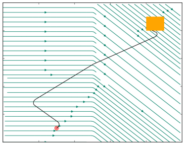
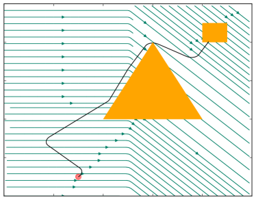
Figure 1: Trajectory found by FS+ for two instances of the Zermelo navigation problem with non-homogeneous wind conditions (arrows show wind direction), and non–convex constraints in the instance on the right. The circle denotes the initial state $s_{0}$, the box the set of goal states $s_{G}$ and the triangle is constraint.

Zermelo’s navigation problem, proposed by Ernst Zermelo 1931, is a classic optimal control problem that deals with a boat navigating on a body of water, starting from a point $s_{0}$ to end up within a designated goal region $s_{G}$. While simple, it has a vast number of real-world applications, such as planning fuel efficient routes for commercial aircraft Soler . (2010). The boat moves with speed $v$, its agility is given by the turning rate $\rho$; both remain constant over time. It is desired to reach $s_{G}$ in the least possible time, yet the ship has to negotiate variable wind conditions, given by the position dependant drift vector $\mathbf{w}(x,y)$ $=$ $\langle u(x,y)$, $v(x,y)\rangle$. States consist of three variables, the current location of the boat $(x,y)\in\mathbb{R}^{2}$ and its heading $\theta$. For fixed heading $\theta$, we have that the location of the boat changes according to the ode:

$$\dot{x} =v\,cos\,\theta+u(x,y)$$ (1)

$$\dot{y} =v\,sin\,\theta+v(x,y)$$ (2)

The agent can steer the boat towards goal states $s_{G}$

$$s_{G}\models x_{G}^{min}\leq x\leq x_{G}^{max}\land y_{G}^{min}\leq y\leq y_{G}^{max}$$

by altering the angle $\theta$ in a suitably defined manner. The function of $\theta$ over time is in effect the control signal Ogata (2010) for this dynamical system. In this paper, we account for the range of possible signals by having instantaneous actions to switch on, off or modulate continuous change over certain state variables. In this example, the agent has available three instantaneous actions $ahead$, $port$, $starboard$ that account respectively for keeping the boat rudder steady, push it towards the right, and to the left. Each of these actions sets an auxiliary variable ctl to the values straight, left and right. These instantaneous actions cannot be executed in any order, so we impose a further (logical) restriction by requiring to keep the rudder straight before being able to push it either towards the left and the right. These actions account for the possible control switches connecting the set of control modes of a Hybrid Automata Henzinger (2000). The variable ctl is then used to define the rate of change of $\theta$ in the following manner: $\dot{\theta}$ $=$ $-\rho$ when ctl $=$ left, $\dot{\theta}$ $=$ $\rho$ when ctl $=$ right, and $\dot{\theta}$ $=$ $0$ otherwise. We note that angles are given in radians.

Time(secs)	0	100	500	600	2030	2130
Action	$starboard$	$ahead$	$port$	$ahead$	$starboard$	$ahead$

Table 1: Plan for the left image on Figure 1, reaching goal area in $2,430$ seconds of simulated time, that required $0.32$ seconds of real time to be computed. $\Delta_{max}$ was set to $100$ seconds, and a zero crossing event was detected at $t=2,030$.

On the left of Figure 1 we can see the trajectory following from the plan in Table 1. The rudder is left alone for quite some time, until the boat almost sails past the goal, and then goes upwind towards $s_{G}$. Global constraints in that scenario require to keep the boat within the bounding box, that coincides with the image extent. On the right in Figure 1 we can see the path that complies with an additional constraint: to stay outside of the golden triangle.

III.   $\smallint$-pddl$+$

The planning language we will use in this work, $\smallint$-pddl$+$, is the result of integrating Functional STRIPS (FSTRIPS) Geffner (2000), and specific fragments of pddl 2.1 Level 2 Fox  Long (2003) and pddl 2.1 Level 5 Fox  Long (2006), also known as pddl$+$. FSTRIPS is a general modeling language for classical planning based on the fragment of First Order Logic (FOL) involving constant, functional and relational symbols (predicates), but no variable symbols, as originally proposed by Geffner, and recently augmented with support for quantification and conditional effects Frances  Geffner (2016), thus becoming practically equivalent to the finite–domain fragment of adl Pednault (1986). Its syntax is essentially the same as that of the “unofficial” revision of pddl, pddl 3.1, first proposed by Helmert 2008 as the official pddl variant of the 2008 International Planning Competition, and fully formalised later by Kovács 2011. To this we have added support for features proposed in pddl 2.1 Level 2 Fox  Long (2003) to handle arithmetic expressions, arbitrary algebraic and trigonometric functions Scala . (2016), and the notion of autonomous processes in pddl 2.1 Level 5 Fox  Long (2006) to account continuous change over time. The implementation of $\smallint$-pddl$+$ is built on top of that in the recent classical planner FS Frances  Geffner (2016).

States, preconditions and goals in $\smallint$-pddl$+$ are described using fluent symbols, whose denotation changes as a result of doing actions or the natural effect of processes over time. Those symbols whose denotation does not change are fixed symbols and include finite sets of object names, integer and real constants, the arithmetic operators ’$+$’, ’$-$’, ’$\times$’, ’$\div$’, exponentiaton, n–th roots, $sin()$, $cos()$ and $tan()$, as well as the relational symbols ’$=$’, ’$>$’, ’$<$’, ’$\geq$’ and ’$\leq$’, all of them following a standard interpretation. Terms, atoms and formulas are defined from constant, function and relation symbols, with both terms and symbols being typed. Types are given by finite sets of fixed constant symbols. Terms $f(\alpha)$, where $f$ is a fluent symbol and $\alpha$ is a tuple of fixed constant symbols, are called state variables, and states are determined by their values. Primitive Numeric Expressions (PNE) Fox  Long (2003) correspond exactly with well formed arithmetic terms combining constants, state variables, arithmetic operators and other functions.

Instantaneous actions $a$ and processes $p$ are described by the type of their arguments and two sets, the (pre)condition and the effects. Action $a$’s preconditions $Pre(a)$ and process $p$’s conditions $K(p)$ are both formulae. Actions and processes differ in the definition of their effects. Action $a$ effects update instantly the denotation of state variables $f(\alpha)$ as a result of applying $a$. Process $p$ effects describe how the denotation of state variables $f(\alpha)$ changes as time goes by. State variables $f(\alpha)$ that appear only in the left hand side of action effects are effectively inertial fluents Gelfond  Lifschitz (1998). On the other hand, those variables $f(\alpha)$ appearing on the left hand side of process effects, and possibly as well in the effects of instantaneous actions, are non–inertial Giunchiglia  Lifschitz (1998) as their denotation can change even when left alone. Formally, the effect of an action $a$ is a set of updates of the form $g(\beta):=\xi_{a}$, where $g(\beta)$ and $\xi_{a}$ are terms of the same type, expressing how $g(\beta)$ changes when $a$ is taken. The effects of a process $p$ is also a set of update rules, but process updates, instead of an assignment, are ode’s $\dot{f}(\alpha)=\xi_{p}$. The value of a time-dependent state variable $f(\alpha)$ after $t^{\prime}-t_{0}$ time units, provided that $p$ is the only process affecting $f(\alpha)$ as prescribed by the update rule $\dot{f}(\alpha)=\xi_{p}$, is given by the following integral equation

$$f^{\prime}(\alpha)=f_{0}(\alpha)+\int_{t_{0}}^{t^{\prime}}\xi_{p}\,\partial t$$ (3)

where $t^{\prime}$ $>$ $t_{0}$ is a positive finite number, $f^{\prime}(\alpha)$ is the value of state variable $f(\alpha)$ at time $t^{\prime}$, and $t_{0}$ is the time associated with the initial conditions $f_{0}(\alpha)$. The type allowed for $f(\alpha)$ and $\xi_{p}$ is restricted to be the real numbers. We impose a further restriction on $\xi_{p}$, namely that it needs to be an integrable function in the interval $[t_{0},t^{\prime}]$, so the rightmost term in Equation 3 is finite.

Global (state) constraints ${\cal C}$ Lin  Reiter (1994) allow to describe compactly restrictions on the values that state variables $f(\alpha)$ can take over time. FS+  currently supports global constraints ${\cal C}$ given as CNF formulae, where each clause $\varphi$ is a disjunction of relational formulae. This allows us to model state constraints similar to those proposed 2014. Since $\smallint$-pddl$+$ supports disjunctive formulae, by extension it accounts for implication as required by Ivankovic’s switched constraints $P\supset S$, where $P$ is a conjunction of literals of so–called primary variables, equivalent to our state variables $f(\alpha)$, and $S$ is an arbitrary formula over so–called secondary variables. However $\smallint$-pddl$+$ cannot represent the latter, as their denotation in any given state is not fixed, as their value is given by those featured in the models (satisfying assignments over $S$) of the constraints.

Last, the planning tasks we consider are tuples ${\cal P}$ $=$ $\langle F,$ $I,$ $O,$ $P,$ $G,$ ${\cal C}\rangle$ where $I$ and $G$ are the initial state and goal formula, $O$ is a set of instantaneous actions, $P$ is a set of processes, ${\cal C}$ is a set of state constraints and $F$ describes the fluent symbols and their types. $I$ must define a unique denotation for each of the symbols in $F$, and satisfy every $C\in{\cal C}$.

IV.   Semantics of $\smallint$-pddl$+$

We first briefly review the semantics of FSTRIPS, following Francès and Geffner 2015; 2016. Then we discuss continuous change on state variables as the timeline is broken into a finite set of intervals, each with an associated set of active processes Fox  Long (2006), or mode Ogata (2010).

The logical interpretation of a state $s$ is described as follows in a bottom–up fashion. The denotation of a symbol or term $\phi$ in the state $s$ is written as $[\phi]^{s}$. The denotation of objects or constants symbols $r$, is fixed and independent from $s$. Objects $o$ denote themselves and the denotation of constants (e.g. $3.14$) is given by the underlying programming language. The denotation of fixed (typed) function and relational symbols can be provided extensionally, by enumeration in $I$, or intensionally, by attaching external procedures Dornhege . (2012). The dynamic part of states $s$ is represented as the value of a finite set of state variables $f(\alpha)$. From the fixed denotation of constant symbols and the changing denotation of fluent symbols $f$ captured by the values $[f(\alpha)]^{s}$, the denotation of arbitrary terms, atoms and formulas follows in a standard way. An instantaneous action $a$ is deemed applicable in a state $s$ when $[Pre(a)]^{s}$ $=$ $\top$, and the state $s_{a}$ resulting from applying $a$ to $s$ is such that, 1) all state constraints are satisfied, $[C]^{s_{a}}$ $=$ $\top$ for every state constraint $C\in{\cal C}$, and 2) $[g(\beta)]^{s_{a}}=[\xi_{a}]^{s}$ for every update $g(\beta):=\xi_{a}$ triggered by $a$, and $[f(\alpha)]^{s_{a}}$ $=$ $[f(\alpha)]^{s}$ otherwise. A sequence of instantaneous actions $act$ $=$ $(a_{1},$ $\ldots,$ $a_{j},$ $\ldots,$ $a_{n})$, $a_{j}\in O$, is applicable in a state $s$ when $[Pre(a_{1})]^{s}$ $=$ $\top$, and for every intermediate state $s_{a_{j}}$, $j>1$, resulting from applying action $a_{j-1}$ in $s_{a_{j-1}}$, it also holds that $[Pre(a_{j})]^{s_{a_{j}}}$. We write $s[act]$ for the state resulting from applying sequence $act$ on state $s$.

Because our time domain, $\mathbb{R}^{+}_{0}$, is dense, the number of states is infinite. We introduce structure into this line by borrowing Fox & Long’s 2006 notion of happenings $\eta$, distinguished points on the time line where an event takes place or an instantaneous action is executed. In between each pair of happenings is a steady interval during which the state evolves continuously according to the set of active processes, or modes, that characterize a dynamical system. We require happenings to exist at any point where processes start or end, thus ensuring the set of active processes is constant throughout each interval.

Formally, a happening $\eta$ is characterised by its timing, $T(\eta)$, mapping $\eta$ to $t\in\mathbb{R}^{+}_{0}$, the state $s(\eta)$ at that time, and a sequence $act(\eta)$ of instantaneous actions applied at the happening. Note that $s(\eta)$ is the state before $act(\eta)$ is applied. An interval is characterised by the two happenings that mark its start and end: $H_{i}=\langle\eta^{-}_{i},\eta^{+}_{i}\rangle$, where the end happening has no associated actions, i.e., $act(\eta^{+}_{i})=\langle\rangle$. The duration of $H_{i}$ is the difference $\Delta_{i}=T(\eta^{+}_{i})-T(\eta^{-}_{i})$ and we assume a finite upper and lower bounds on the duration of each interval, i.e., $\Delta_{min}$ $\leq$ $\Delta_{i}$ $\leq$ $\Delta_{max}$, are provided as part of the problem description. The lower bound $\Delta_{min}$ can indeed be set to $0$, but in that case we observe that introduces the possibility of plans with infinite length, their execution being referred to as a Zeno’s execution in existing literature in hybrid control theory Goebel . (2009). The values of state variables $f(\alpha)$ at the start of the interval $H_{i}$ are given by the state $s^{i}_{0}$ that results from applying the sequence of actions $act(\eta^{-}_{i})$ associated with the start happening to the state $s(\eta^{-}_{i})$, i.e. $s^{i}_{0}\equiv s(\eta^{-}_{i})[act(\eta^{-}_{i})]$. During the interval $H_{i}$, continuous state variables may be affected by the set of processes that are active in $H_{i}$. The state at the end of $H_{i}$, $s(\eta^{+}_{i})$, is defined by integrating the active processes’ effects, following the general form of Equation 3. We define the set of active processes $\mu_{i}\subseteq P$, or mode, associated with interval $H_{i}$, as those whose conditions hold in the state at the interval’s beginning:

$$\mu_{i}=\{p\,\mid\,p\in P,\,\,s^{i}_{0}\models K(p)\}$$

We note that $\langle s^{i}_{0},\mu_{i}\rangle$ is the dynamical system associated to $H_{i}$. Several active processes can affect the same state variable $f(\alpha)$. Recall that process effects specify the rate of change: we follow the standard convention that process effects superimpose, by adding together the rates of change of all active processes affecting $f(\alpha)$ Ogata (2010). The value of state variable $f(\alpha)$ in state $s(\eta^{+}_{i})$ is then given by

$$[f(\alpha)]^{s(\eta^{+}_{i})}=[f(\alpha)]^{s^{i}_{0}}+\int_{T(\eta^{-}_{i})}^{T(\eta^{+}_{i})}\sum_{p\in{\cal R}_{f(\alpha)}}\delta_{p}^{i}\,\,\xi_{p}\,\,\partial t$$ (4)

where ${\cal R}_{f(\alpha)}\subseteq P$ is the set of processes $p$ where $f(\alpha)$ appears on the left hand side of some effect $\xi_{p}$, and the activation variable, $\delta_{p}^{i}$, for each process $p$ is the characteristic function of the mode $\mu_{i}$, meaning that $\delta_{p}^{i}=1$ if $p\in\mu_{i}$ and $0$ otherwise. Equation 4 can be simplified. First, note that as long as $\mu_{i}$ remains stable, that is, the set of active processes does not change over the duration of interval $H_{i}$, $\delta_{p}^{i}$ does not depend on time $t$. Second, the restriction on $\xi_{p}$ imposed in the previous Section, i.e. that $\xi_{p}$ is a continuous function over $[T(\eta^{-}_{i})$, $T(\eta^{+}_{i})]$, enables the direct application of Fubini’s Theorem 1907. Provided that $\mu_{i}$ is stable we can rewrite Equation 4 as

$$[f(\alpha)]^{s(\eta^{+}_{i})}=[f(\alpha)]^{s^{i}_{0}}+\sum_{p\in{\cal R}_{f(\alpha)}\cap\mu_{i}}\int_{T(\eta^{-}_{i})}^{T(\eta^{+}_{i})}\xi_{p}\partial t$$ (5)

Next, we define a condition that implies the interval $H_{i}$ is stable, i.e., that $\mu_{i}$ does not change during $H_{i}$. To do this, we verify that none of the following happens at any point $t$ $\in$ $[T(\eta^{-}_{i}),T(\eta^{+}_{i})]$: (1) the truth of the conditions $K(p)$ of some process $p\in P$ changes, (2) some state constraint $C\in{\cal C}$ is violated, and (3) we do not “shoot through” sets of states where the goal $G$ is true. The absence of each of these events can be expressed as a condition, the conjunction of these three conditions is the invariant formula

$${\cal I}(H_{i}):\neg G\land\bigwedge_{p\in\mu_{i}}K(p)\land\bigwedge_{p^{\prime}\in P\setminus\mu_{i}}\neg K(p^{\prime})\land\bigwedge_{C\in{\cal C}}C$$ (6)

Howey  Long (2003); Howey . (2005). If the invariant ${\cal I}(H_{i})$ holds throughout $H_{i}$, then $H_{i}$ is stable. Note that sub-formulae of ${\cal I}(H_{i})$ that mention only state variables $f(\alpha)$ not affected by any process always remain true over $H_{i}$. Following Shin & Davies’ 2005, we refer to a change in the truth value of ${\cal I}(H_{i})$ as a zero crossing event.

Definition 1.

(Zero Crossing Event) Let $H_{i}$ be a interval with timings $T(\eta^{-}_{i})$ and $T(\eta^{+}_{i})$, and invariant ${\cal I}(H_{i})$. A zero crossing event occurs whenever for some $t^{\prime}$ s.t. $T(\eta^{-}_{i})$ $<$ $t^{\prime}$ $<$ $T(\eta^{+}_{i})$, ${\cal I}(H_{i})$ is false.

Definition 2.

(Steady Intervals) Let $H_{i}$ be a interval with timings $T(\eta^{-}_{i})$ and $T(\eta^{+}_{i})$, state $s^{i}_{0}$ and mode $\mu_{i}$. Whenever zero crossing event occurs for some $t^{\prime}$ s.t. $T(\eta^{-}_{i})$ $<$ $t^{\prime}$ $<$ $T(\eta^{+}_{i})$, then the interval $H_{i}$ is a steady interval, whose dynamics are fully described by the dynamical system $\langle s^{i}_{0},\mu_{i}\rangle$.

We are now ready to define what is a solution for our planning tasks. A valid plan $\pi$ for hybrid planning task ${\cal P}$ is a finite sequence

$$\pi=(H_{0},H_{1},\ldots,H_{i},\ldots,H_{m})$$

of steady intervals $H_{i}$, such that (1) $s(\eta^{+}_{m})\models G$, and (2) $T(\eta^{-}_{m})=T(\eta^{+}_{i-1})$. The optimality of plans depends on the metric the modeller specifies for ${\cal P}$ as evaluated on $s(\eta^{+}_{m})$: our extended FSTRIPS language, like pddl 3.1, enables the modeller to specify both obvious metrics such as the overall duration of $\pi$ (i.e. $\sum\Delta_{i}$) and more intricate ones as needed.

i.   Comparison with pddl$+$

The planning language we define is very similar to, and certainly owes many of its core concepts to, the specification of pddl$+$  given by Fox & Long  2006. However, it separates in two ways, in the interpretation of plans and not accounting for the pddl$+$ notion of events completely.

First, we consider only the computation of plans with finite duration and representation, consisting of a finite but unbounded number of happenings. Our interpretation of happenings is that they break the continuous timeline into a finite sequence of intervals during which the continuous effects on state variables are stationary. The number of states in each interval is infinite, but all such intermediate states are cataloged implicitly by the states at the happenings that mark the extent of the interval Pednault (1986).

Second, we allow the planner to execute a finite but unbounded sequence of instantaneous actions at a happening $\eta$ without any restriction, such as commutativity, on their effects. This allows us to model, for instance, the network of valves in the rocket engine discussed in the classic work of Williams & Nayak 1996 without an explosion in the number of instantaneous actions required to represent all possible combinations of valve positions. In contrast, pddl$+$  mandates a non-zero time separation (known as the “$\epsilon$”) between non-commutative instantaneous actions. This restriction is motivated by the assumption that actions, although modelled as instantaneous, cannot actually be executed in zero time Fox  Long (2006). However, for those cases in which a temporal separation, or “cool down” period, between actions is motivated by the application domain, this can be modelled (using an auxiliary process representing a timer, for instance) also in our setting. Thus, no expressivity is lost when it comes to model limitations in the execution of plans.

Finally pddl$+$  considers events to be “first–class citizens” in the language, with semantics best described as “exogenous” instantaneous actions, rather than implicitly defined as points where invariant conditions change. Although events are in some cases a natural and convenient modeling device, some of their effects can also be captured by introducing suitably defined global constraints or compiled into process preconditions. For instance in the Mars Solar Rover domain proposed by 2005, one can do away with the events sunset and sunrise by having a global timer for the whole day, and modifying accordingly the preconditions of the processes day time and night time. This also avoids some of the problems Fox et al observe to be associated with plan validation in the presence of events. On the other hand, uses of events to model spontaneous changes in the dynamics, are not accounted for. A natural and familiar example of such phenomena is that of ellastic collisions between bodies with the same mass, where the direction of acceleration changes as consequence of the collision. Accounting for these would be necessary to model accurately as a hybrid domain real-world tasks such as playing solitaire pool.

V.   Branching and Computing Successor States

As outlined in the Introduction, FS+ searches for plans $\pi$ of hybrid planning task $P$ via forward search over a deterministic state model $M({\cal P})=\langle S$, $s_{I}$, $A^{\prime}$, $S_{G}$, $App$, $f$ $\rangle$ where each element is defined as follows. The state space $S$ is given by all the possible combinations of denotations for fluents $F$ plus an auxiliary state variable $t()$ to represent the location of states $s$ on the time line. Actions $A^{\prime}=$ $O$ $\cup$ $\{sim\}$ include the instantaneous actions $O$ in ${\cal P}$ and a $sim$ action that updates $t()$ and simulates the world dynamics as given by the continuous effects of processes $P$. Goal states $S_{G}\subseteq S$ are those states $s$ s.t. $[G]^{s}=\top$; $s_{I}$ is like $I$.The applicability function $App$ corresponds exactly with the notion of applicable actions discussed in the previous Section, while $sim$ actions can be applied in every state $s\in S$. $f(a,s)=s_{a}$ for instantaneous actions $a$; we devote the rest of this Section to define $f(sim,s)$. Solutions to $M({\cal P})$ are paths $\pi^{\prime}$ $=$ $(a_{0}$, $\ldots$, $a_{n})$ connecting $s_{I}$ with some $s\in S_{G}$. The plan $\pi$ made up of intervals $H_{j}$ is obtained from paths $\pi^{\prime}$ by observing that (1) for every action $a_{j}$ $=$ $sim$ action in $\pi^{\prime}$, there is an interval $H_{j}$ in $\pi$, (2) the timing of happening $\eta^{-}_{j}$ is $[t()]^{s_{l}}$, where $s_{l}$ $=$ $s_{0}$ or $s_{l}$ = $f(a_{l},s_{l-1})$, $a_{l}$ $\in$ $\pi^{\prime}$ $a_{l}$ $=$ $sim$, $l<j$, (3) the timing of happening $\eta^{+}_{j}$ is $[t()]^{s_{j}}$, $s_{j}$ $=$ $f(s_{j-1},sim)$, and (4) $act(\eta^{-}_{j})$ $\subset$ $\pi^{\prime}$, defined as $act(\eta^{-}_{j})$ $=$ $($ $a_{k}$, $\ldots$, $a_{j-1}$ $)$, $k=0$ or $a_{k-1}$ $=$ $sim$. As suggested by this mapping of paths between initial and goal states in $M({\cal P})$ into sequences of intervals $H_{i}$, the action $sim$ (1) predicts successor states by solving Equation 5 for every state variable $f(\alpha)$ appearing on the left–hand side of effects of processes $p$ $\in$ $\mu_{i}$, and (2) validates the assumption that $\mu_{i}$ is stable checking whether for some $t_{zc}$ in the interval $[T(\eta^{-}_{i})$, $T(\eta^{-}_{i})$ $+$ $\Delta_{max}]$ the truth of ${\cal I}(H_{i})$ changes. When that is the case, auxiliary variable $t()$ is set to $t_{zc}$ instead of $T(\eta^{-}_{i})$ $+$ $\Delta_{max}$, in turn setting $T(\eta^{+}_{i})$ to $t_{zc}$ as well.

We note that both of these problems cannot be solved exactly in general, as both state prediction, or general symbolic integration, and validation, or finding roots of real–valued functions Howey  Long (2003), can be shown to be undecidable by Richardson’s Theorem 1968. Consequently, it will never be possible to guarantee that plans are valid, but that is not necessary to compute plans that are accurate enough to inform the solution of real-world engineering problems. While exact, general solutions are out of reach, we can turn to numerical approximation methods for both prediction and validation. We discuss how we approximate the prediction of successor states and their validation next.

i.   Related Work: Analytical Solutions and Linear Dynamics

The implications of Richardson’s Theorem on the validity of plans are indeed quite negative, and it has motivated the planning community to look into less expressive, yet still powerful and widely applicable, fragments of hybrid planning, where the form of processes effects is restricted in some way. We devote this Section to briefly discuss existing work on a fragment that, while still undecidable, does not require to explicitly discretise time.

A substantial part of the existing literature on hybrid planning studies domains where the right–hand side $\xi_{p}$ of processes $p$ in modes $\mu_{i}$ reachable from the initial state, and hence the dynamical systems associated with such modes $\langle s^{i}_{0},\mu_{i}\rangle$, has a specific form: that of general linear expressions,

$$\xi_{p} :\,\,b_{p}+\sum_{f(\alpha)\in F}w_{f(\alpha)}^{p}f(\alpha)$$ (7)

In that case, the combined effects of processes in $\mu_{i}$ can be written compactly in matrix form as follows:

$$\dot{\mathbf{x}}=\mathbf{A}\mathbf{x}+\mathbf{b}$$ (8)

where $\mathbf{x}$ is made of (time–varying) state variables $f(\alpha)$ and both $\mathbf{A}$ and $\mathbf{b}$ follow from the coefficients in Equation 7. The dynamical systems Equation 8 accounts for are a useful and well known class of dynamical systems, known as Linear Time–Invariant (LTI) systems Scheinerman (2001); Ogata (2010), for which there exists an analytical solution to Equation 8. LTI systems are good models for a huge range of domains Löhr . (2012), yet still lack generality since linear approximations of physical processes are not always reasonable. From a practical standpoint, solving the initial value problem amounts to computing the exponential of matrix $\mathbf{A}$. Matrix exponentiation is a non–trivial linear algebra problem Horn  Johnson (2013), that needs to be solved for every possible system $\langle s^{i}_{0},\mu_{i}\rangle$. Existing approaches rely on precomputing the closed form for Equation 8, something which is tricky in domains like McDermott’s Convoys 2003 where enumeration can be impractical.

ii.   To Successor States via Numerical Integration

Computing the state corresponding to the happening $\eta^{+}_{i}$ requires $sim$ to solve the initial value problem Butcher (2008), for the dynamical system $\langle s^{i}_{0},\mu_{i}\rangle$ associated with the interval $H_{i}$. FS+ does so relying on numerical integration methods Butcher (2008) that do not require syntactic restrictions on the effects $\xi_{p}$ of processes $p\in P$ in order to be applicable. This generality comes at a cost: since numerical integration relies on discretization of the free variable, time $t$ in this case, and we need to introduce a new parameter, $\Delta z$, the simulation step. The computation of the state $s(\eta_{i}^{+})$ for a given interval $H_{i}$, proceeds as follows. We start observing that given any happening $\eta$, a mode $\mu_{i}$ and the state $s(\eta)$, the state $s(\eta^{\prime})$ of another happening $\eta^{\prime}$ s.t. $T(\eta^{\prime})$ $=$ $T(\eta)+\Delta z$ is defined as

$$s(\eta^{\prime})=\Phi[s(\eta),\mu_{i},\Delta z]$$

where $\Phi[\cdot]$ is the specific numerical integration method being used to predict the values of state variables $f(\alpha)$ being changed by processes $p\in\mu_{i}$. Computing the state $s(\eta_{i}^{+})$ amounts to integrate Equation 5 over intervals of duration $\Delta z$, and repeat this $k$ times where

$$k=\left\lfloor\frac{T(\eta_{i}^{+})-T(\eta_{i}^{-})}{\Delta z}\right\rfloor$$

Whenever $k$ $\Delta z$ $<$ $\Delta_{i}$ an additional call to the integration method $\Phi[\cdot]$ using $\Delta z^{\prime}$ as the simulation step is needed and

$$\Delta z^{\prime}=T(\eta_{i}^{+})-(T(\eta_{i}^{-})+k\Delta z)$$

The simplest integrator $\Phi[\cdot]$ implemented in FS+ is the Explicit Euler Method Butcher (2008), that determines the values of $f(\alpha)$ in state $s_{k}$ following Equation

$$[f(\alpha)]^{s(\eta^{\prime})}=[f(\alpha)]^{s(\eta)}+\Delta z\sum_{p\in\mu_{i}}[\xi_{p}]^{s(\eta)}$$ (9)

which is the recurrence relation for integral Equation 5. The convergence of numerical integration methods like the one in Equation 9 is very sensitive to the choice of $\Delta z$, and for non–linear $\xi_{p}$ these methods can be easily shown to diverge even for small values of $\Delta z$. On the other hand, more robust numerical integration methods, such as the Runge–Kutta integrators Butcher (2008), are significantly more complicated than Equation 9 yet still much cheaper than matrix exponentiation. Amongst these, FS+ currently implements the midpoint rule, the 2nd order Runge–Kutta integrator that Butcher refers to as $RK22$. FS+ also implements the iterative or multi–step Implicit Euler method

$$[f(\alpha)]^{s_{j+1}(\eta^{\prime})}=[f(\alpha)]^{s(\eta)}+\Delta z\sum_{p\in\mu_{i}}[\xi_{p}]^{s_{j}(\eta^{\prime})}$$ (10)

where $[f(\alpha)]^{s_{0}(\eta^{\prime})}$ is given by Equation 9, and iteration continues until the following fixed–point is reached:

$$|\,[f(\alpha)]^{s(\eta^{\prime})}_{j+1}-[\xi_{p}]^{s(\eta^{\prime})}_{j}\,|<\epsilon$$ (11)

Last, for problems where all process effects are linear expressions, we note that the “messy” numerical integrator $\Phi[\cdot]$ currently available in FS+ could be readily substituted with the analytical solution of the LTI system given by $\mu_{i}$, calling an external solver online instead of doing so as pre–processing step, during the search. Such a change would entail significant gains in precision, but we suspect the cost of computing the analytical solution would have a significant negative effect on run–times.

iii.   Testing for Zero Crossings

The invariant ${\cal I}(H_{i})$ is a conjunction of parts, each of which can be evaluated separately. Some parts may be disjunctive (thus non-convex) as a result of negating conjunctive goals $G$ or process conditions $K(p)$ Howey  Long (2003), or from disjunctive global constraints. Recall, however, that the main aim of validation is to prove the absence of a zero-crossing event in the simulated time interval. This allows us to simplify the problem by testing necessary conditions for a zero-crossing event to occur; if those are not satisfied, we can conclude no such event happened, and hence that the interval is steady. If a zero-crossing event may have occured, it is sufficient to find an time point $t$ in the interval such that the event is necessarily after $t$. The length of the steady interval is then shortened, and the planner inserts a new happening at $t$ from which it can branch.

To validate a disjunctive formula $\varphi=\phi_{1}\lor\ldots\lor\phi_{l}$ over an interval starting from state $s$, we test instead $\varphi^{s}=\bigwedge_{j\text{s.t.}s\models\phi_{j}}\phi_{j}$, that is, the conjunction of the disjuncts that are true in $s$, since the falsification of at least one of those disjuncts is a necessary condition for $\varphi$ to become false. After strengthening ${\cal I}(H_{i})$ in this fashion, we introduce $k$ happenings $\eta_{i}^{j}$ with timings $T(\eta_{i}^{j})$ $=$ $T(\eta_{i}^{-})$ $+$ $j$ $\Delta z$, and $T(\eta_{i}^{-})$ $+$ $k$ $\Delta z$ $<$ $T(\eta_{i}^{+})$, and states resulting from calls to an integrator $\Phi[\cdot]$ using a finer grained simulation step $\Delta h$. Where $\xi_{l}$, $\xi_{r}$ are arithmetic terms and $\oplus$ is a relational symbol, the truth of an atomic formula $\psi=\xi_{l}\oplus\xi_{r}$, in state $s$ is tied to the sign of the function $f_{\psi}$

$$f_{\psi}(s)=[\xi_{l}-\xi_{r}]^{s}$$ (12)

– $\psi$ can only change from true to false if $f_{\psi}(s)$ changes sign. Whether this occurs in the interval between two consecutive happenings $\eta_{i}^{j}$, $\eta_{i}^{j+1}$ can be determined by direct application of the following classical result from mathematical analysis:

Theorem 3.

(Intermediate Value Theorem) Let $f$ be continuous on the closed interval $[a,b]$. If $f(a)$ $\leq$ $y$ $\leq$ $f(b)$ or $f(b)$ $\leq$ $y$ $\leq$ $f(a)$ then there exists point $c$ such that $a$ $\leq$ $c$ $\leq$ $b$ and $f(c)$ $=$ $y$.

We observe that (1) $f_{\psi}$ is a continuous function, following from the constraint on effects of processes $\xi_{p}$ to be integrable, and (2) if $f_{\psi}(\eta_{i}^{j})$ $<$ $0$ ($>$ $0$) and $f_{\psi}(\eta_{i}^{j+1})$ $>0$ ( $<$ $0$), then there necessarily exists a happening $\eta_{zc}$, $T(\eta_{zc})\in[T(\eta_{i}^{j}),T(\eta_{i}^{j+1})]$ such that $f_{\psi}(\eta_{zc})$ $=$ $0$, i.e. a zero–crossing event for $\psi$ takes place at time $T(\eta_{zc})$. The earlier strengthening of disjunctions implies that $\varphi^{s}$ is falsified as soon as this happens for any atomic formula $\psi$ is. In this case, the interval $H_{i}$ is shortened by setting $\eta^{+}_{i}=\eta^{j}_{i}$.

The treatment of disjunctive invariants means that happenings may be inserted where not truly needed, since a disjunction can remain true even if one of its disjuncts is falsified. This may lead to a deeper search than necessary, but any path found will still be valid. If the dynamics in the interval oscillate rapidly, the indicator function $f_{\psi}$ may change sign several times within the validation time step $\Delta h$; thus, the procedure may also fail to detect a zero-crossing event. As noted earlier, this is an unavoidable consequence of the undecidability of the root-finding problem in general.

VI.   Searching for Plans

In the previous Section we have mapped our take on planning over hybrid systems into the problem of finding a path in a deterministic state model $M({\cal P})$. This enables us to use, off–the–shelf without modifications, any known blind or heuristic search algorithm, such as Breadth–First Search or Greedy Best First Search, to seek plans. Still, heuristic guidance is essential for scaling up over these domains: none of the instances discussed in the next Section are solvable by Breadth–First Search when doing on–line validation of successor states. In order to obtain a heuristic, FS+ follows Scala et al. 2016, and compiles away processes $p$ as instantaneous actions $a_{p}$. That is, for each update rule $\dot{f}(\alpha):=\xi_{p}$ we introduce an action effect that mimicks Equation 9

$$f(\alpha):=f(\alpha)+\Delta_{max}\,\xi_{p}$$ (13)

where $\Delta_{max}$ is the planning step. Then, on the resulting classical planning task $P_{num}$, which is like ${\cal P}$ but with $P$ $=$ $\emptyset$, we apply a novel heuristic, $h_{\text{{\small FS+}}}$, that integrates two recent works. One is the Aibr relaxation Scala . (2016) that generalizes the notion of value–accumulation semantics  Gregory . (2012) to dense intervals defined over numeric variables. The other is the Crpg heuristic by Francès and Geffner 2015, developed to exploit the structure of planning tasks exposed by FSTRIPS. $h_{\text{{\small FS+}}}$ extends the constraint language supported by Crpg to support real–valued variables, defined over intensionally represented domains, i.e. intervals instead of sets. Scala et al ’s convex union operator is then used to succinctly accumulate the intervals revised after applying actions on each layer of the Crpg, thus propagating upper and lower bounds over numeric variables along with atomic formulae across layers. $h_{\text{{\small FS+}}}$ estimate corresponds to the number of actions and processes that are needed to get into a layer of the Crpg where the goal is satisfied. FS+ relies on the Cp framework GeCode as the latest versions of Francès and Geffner 2016 planners do.

VII.   Experimental Evaluation

Domain	P & G	Dyn	Source
Agile Robot	L	L, H	Löhr (2014)
Orbital Rendezvous	L	L, G	Löhr (2014)
Convoys	L	L,NH	McDermott (2003)
Intercept	NL	L, NH	Scala . (2016)
Zermelo	L	NL	Zermelo (1931)
1D Powered Descent	L	L, G	2016
Non Linear Car	L	NL	Bryce . (2015)
Dino’s Car	L	NL	Piotrowski . (2016)

Table 2: Taxonomy of domains according to expressions, in preconditions, process conditions, goals (P & G) and process effects (Dyn), being linear (L) or non–linear (NL) . We further distinguish three different sub-clases for Linear dynamics: general (G), homogenous (H), non–homogeneous (NH). See text for details.

In order to evaluate FS+ we have selected a number of benchmarks already proposed in the literature on hybrid and numeric planning, as well as the Zermelo’s navigation problem (Zermelo) discussed in Section II. The criterion used to select benchmarks was first and foremost to consider a diverse representation of the kind of linear and non–linear that can be modeled with $\smallint$-pddl$+$, and pddl$+$, with non–trivial branching factor. Table 2 lists the domains considered, along with the pointers to the publication describing them and a classification of their dynamics. Benchmarks are considered to have linear dynamics (L) when every reachable $\langle s^{i}_{0},\mu_{i}\rangle$ is a LTI system. Two special cases of LTI systems Scheinerman (2001) are considered, namely, homogenous (H) systems, where $\mathbf{b}$ $=$ $\mathbf{0}$, and non–homogenous (NH) systems, where $\mathbf{A}$ $=$ $\mathbf{0}$. Convoys and Non Linear Car instances were taken from Scala . (2016). For two of the domains, namely Agile Robot and Orbital Rendezvous, no pddl$+$ formulation was available for us to use, so we coded them up from scratch following Löhr’s description in his PhD dissertation 2014.

We next briefly discuss some interesting features of the domains and how events and durative actions were handled when present in existing pddl$+$ formulations. In McDermott’s Convoys the number of possible modes is given by the possible combinations of assignments of convoys and point-to-point routes in the navigation graph. This potential combinatorial explosion was something intended, as McDermott’s points in his paper 2003. Orbital Rendezvous required us to compile away the durative actions present in Löhr’s model following the discussion in Section 4 of Fox & Long paper on pddl$+$ 2006, but instead of introducing a “stop“ action, we introduce an auxiliary “timer” variable set by the “start” action, whose value decreases as an effect of the process being triggered. Besides Löhr’s five hand crafted instances, we have generated a number of random ones, following a Gaussian distribution around the initial states featured in Löhr’s instances. We report the results of the planners on each set to show the robustness of the planners when slight perturbations are introduced in initial states. Last, the instances of Agile Robot we consider have no obstacles, but do have dead–ends: when (if) the robot velocity reaches the value of $0$, there is no way to put it back into motion. Events in the domains Powered Descent and Dino’s Car were used to introduce dead end states when the trajectories induced by plans hit a region of the state space where a given property $\phi$ holds. We translated these directly as global constraints $\neg\phi$, doing away with no longer necessary auxiliary predicates present in Piotrowski’s model that enable actions and processes. Conversely, global constraints $\psi$ in Zermelo, Agile Robot, Orbital Rendezvous and Non Linear Car were translated into events with precondition $\neg\psi$ and effects that delete irrevocably auxiliary predicates in the preconditions of actions and processes. FSTRIPS and pddl$+$ domains and sample instances.

			UPMurphi			DiNo			ENHSP			FS+ RK22,NV			FS+ RK22
Domain	$\Delta_{max}$	I	S	R	D	S	R	D	S	R	D	S	R	D	S	R	D
Agile Robot	0.5	100	82	1.11	14.46	82	21.10	18.68	100	10.55	8.5	100	0.47	7.0	100	8.00	6.5
	1.0	100	0	n/a	n/a	0	n/a	n/a	0	n/a	n/a	100	0.14	10.0	97	0.89	7.4
Convoys	1	6	2	2.58	18.50	3	99.31	15.33	6	4.21	11.7	6	3.57	12.3	6	4.78	11.6
Dino Car	1	10	10	1.78	15.00	10	176.00	16.80	10	0.07	12.0	10	0.01	11.0	10	0.03	11.0
Intercept	0.1	10	12	204.16	62.17	0	n/a	n/a	10	5.68	10.6	8	39.00	10.3	10	28.28	10.4
	1	10	0	n/a	n/a	0	n/a	n/a	0	n/a	n/a	0	n/a	n/a	10	85.93	10.5
Non Linear Car	1	8	10	1.78	15.00	10	176.00	16.80	8	0.55	10.4	8	1.68	10.5	8	0.72	10.2
Orb. Rend. (Löhr)	100	5	1	35.92	9900	0	n/a	n/a	5	0.36	2300.0	5	0.26	2900.0	5	0.46	2223.4
(Random)	100	100	1	34.20	2100	0	n/a	n/a	100	0.31	2104.0	100	0.09	2534.0	100	0.34	2059.8
Powered Descent	1	20	10	209.64	26.10	18	47.25	40.33	20	1.99	31.4	19	2.75	31.1	16	1.80	28.5
Zermelo	100	100	0	n/a	n/a	0	n/a	n/a	92	6.16	2284.8	98	1.04	2225.5	94	1.23	2098.9

Table 3: Coverage of UPMurphi, DiNo, ENHSP and FS+ over the domains in Table 2. Timeout (TO) was set to $1,800$ seconds and physical memory limited to $4$ GBytes. $\Delta_{max}$ is the planning time step used, $I$ is the number of instances for each domain, $S$ is the number of instances solved by the planner, $R$ is the average run-time (in seconds) and $D$ is the average duration of the plans in seconds for all the domains but Convoys, where it is given in hours. UPMurphi, DiNo and ENHSP all use $\Delta_{max}$ as their discretisation step. Two variants of FS+ are considered, FS+ _RK22 uses the $RK22$ integrator checking for zero crossings of Equation 6, FS+ _RK22,NV uses the same integrator but does not check for zero crossings. $\Delta z$ is set to $0.1\Delta_{max}$ for the FS+ planners. NS indicates that the planner did not support the domain, “Crashes” that the planner crashed during execution.

We have compared FS+ with four state–of–the–art hybrid planners, UPMurphi DellaPenna . (2009), DiNo Piotrowski . (2016), ENHSP Scala . (2016) and SMTPlan+ Cashmore . (2016). Table VII shows coverage and run times for the three first planners. We have only managed to run SMTPlan+ on Intercept, where it solved all the instances in less than a second. Its authors reported, via personal communication, that dynamics other than non–homogenous linear ($NH$) are not supported at the time of writing this. In Convoys SMTPlan+ failed to generate a formula. We used the planning step $\Delta_{max}$ as the discretization parameter for UPMurphi   DiNo and ENHSP. The values for $\Delta_{max}$ follow either from the values used in the papers discussing each domain, in the case of Zermelo we performed an analysis similar to the one perfiormed by Piotrowski’s for Powered Descent 2016. In addition, DiNo requires bounds on plan duration to be supplied as a parameter for its heuristic estimator. We used the values given by Piotrowski et al when available, otherwise we used the duration obtained by the FS+ planner. We show in Table VII two of out of six configurations of FS+ tested, where we considered each of the three integration methods implemented, turning on and off the testing for zero crossings. The two configurations chosen showed the best trade–off between run times, coverage and plan duration over these benchmarks. In all cases we used a generic implementation of Greedy Best First Search.

Table VII shows that the two best performing FS+ configurations clearly dominate UPMurphi and DiNo on every domain but Powered Descent. We consider this results to be indicative, we have observed the performance of UPMurphi and DiNo to be very sensitive to the parameters used to discretise time and any numeric variables. Compared with ENHSP, we can see that by doing considerably more computation while searching for plans, the FS+ planners have similar or superior runtimes and coverages across all the domains considered. Also, FS+ plans reach goal states faster when on–line zero crossing detection is enabled. This provides evidence that the numerical integration and on–line discretization mechanisms proposed in this planner can pay off over a broad class of domains. We also note that the FS+ planners can solve the same domains by increasing $\Delta_{max}$, doing less work to find better plans in Agile Robot, but in three instances where our dynamic discretization strategy results in very deep searches, and solving all instances of Intercept. Somewhat surprisingly, $\text{{\small FS+}}_{RK22}$ solves less problems than $\text{{\small FS+}}_{RK22,NV}$ in Agile Robot, when $\Delta_{max}$ $=$ $1$. Testing for zero crossings not only avoids generating unsound plans, sometimes resulting on the search abandoning a very deep plan prefix, in which case $\text{{\small FS+}}_{RK22}$ finds fewer plans as it times out. On other occasions, it does create opportunities to reach a goal state by interrupting an interval $H_{i}$, bringing about shallower searches, in which case $\text{{\small FS+}}_{RK22}$ finds more plans. The latter follows from considering zero crossings for the goal formula in Equation 6 and preventing the planner from overshooting and ruling out plan prefixes which result in “orbiting” the goal region. The most dramatic impact of this observation becomes apparent in the Intercept when $\Delta_{max}$ is $1$. We consider this to be a strength of our approach, and also highlights the limitations of the classic search method used, Greedy Best First Search.

Validation of hybrid plans is still problematic, and warrants further attention from the community. The well–known hybrid plan validator Val Howey . (2005) does not handle most of the types differential equations listed in Table 2. Of the domains listed there, we could only use Val on Intercept. In the rest, we verified offline the plans generated by FS+ with our own validator, which is FS+ itself loading up a given plan like Val does and executing it using the most precise integrator available, the Implicit Euler method in Equation 10 and the smallest $\Delta_{max}$ allowed by the precision of the floating point representation used, $0.001$. This value follows from multiplying by $100$ the smallest value of $\Delta z$ for which the C++ type float produces reliable results,$\leavevmode\nobreak\ 1e^{-5}$. We found no invalid plans for the $\text{{\small FS+}}_{RK22}$ configuration. For $\text{{\small FS+}}_{RK22,NV}$ configuration, that does not perform any checks for zero crossings for the invariant in Equation 6, we did indeed detect invalid plans being generated in every of the domains considered.

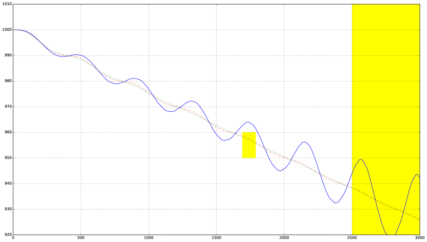
Figure 2: Convergence of integration methods on the Sailplane domain, that implements the phugoids model of glider flight. Lines represent the trajectory that follows from the plans considered during search. Trajectories induced by Explicit Euler (solid line), $RK22$ (dashed) and Implicit Euler (dotted) is shown. See https://goo.gl/SdwafF for details and the text for discussion. $x$-axis indicates distance from the origin and the $y$-axis is the height of the glider, both measured in meters. Curves represent the trajectory of the glider as predicted by each numerical integration method.

The challenge posed by arbitrary, non–trivial non–linear dynamics is illustrated next. Figure 2 depicts the trajectories obtained with the numerical integrators discussed in Section V over a domain that makes apparent the trade-off between good convergence properties of the numerical integrator and run time. $\Delta z$ is set to $0.5$ in all three cases. We note that successor generation of UPMurphi, DiNo and ENHSP can be interpreted as using the Explicit Euler method directly with fixed $\Delta z$ $=$ $\Delta_{max}$. When the set of goal states is the larger rectangle on the right hand side of Figure 2 the three integrators discussed seem equivalent: they all result in trajectories that reach the goal. But, when the set of goal states is the smaller rectangle, none of these planners would “see” the goal without considerably reducing the rates at which time is discretized. While the explicit Euler method requires trivial amounts of computation, the trajectories obtained by the Runge–Kutta and Implicit Euler methods in Figure 2 are significantly more expensive, with the Implicit Euler method being about $100$ times slower than the Runge–Kuta method we have implemented, which in turn is $3$ times slower than the Explicit Euler method.

VIII.   Discussion

To sum up, this paper develops formally and practically the notions of on–line numerical integration and dynamic discretization in the context of hybrid planning. The resulting planner, FS+, seeks plans by means of heuristic forward search, and is shown to perform robustly and compare favorably with existing similar planners, over a varied set of benchmarks. We propose alternative semantics for hybrid planning, but the purpose of doing so is not to supersede pddl$+$, but rather, to offer a complementary and useful view on the problem, compatible with existing tools to a great degree. We hope this work will help to draw interest from the greater classical planning community onto this very challenging and interesting form of planning, since we think the model presented in Section V suggests that existing techniques developed for classical propositional planning could be adapted to operate on it.

In this work we have only accounted partially for natural examples motivating the use of pddl$+$ events to model real–world control tasks, we look forward to incorporate events as future work, introducing syntactic restrictions to avoid complicating even more the validation of plans. Further exploring the impact of syntactic restrictions looks to us as a promising future line of work, which allows to take a more positive look at the questions posed by the difficulties of validating the plans produced than initially suggested by the somewhat discouraging Richardson’s undecidability results. First, it is obvious to us that fragments of hybrid planning that are decidable do exist. For instance, those domains where the expressions used in the effects of processes are such that the trajectory induced by plans for specific tasks can be mapped into the traces of Timed Automata Alur  Dill (1994). That opens up the possibility that planning algorithms can be used to solve realizability queries over such automata scaling up as the number of state variables grows, better than existing approaches. Second, and after acknowledging that there is a temporal planning problem in every hybrid one, it becomes apparent to us that a significant part of global constraints and preconditions typically featured by many domains are about the timing of actions or, indirectly, of events which result in sets of simple linear numeric constraints the planner needs to check for zero crossings. In that case, zero crossing checking can be done symbolically as first shown by Shin & Davies’ in their planner  TM-LPSAT 2005. This suggests in turn that the on-line validation techniques described in Section V could be specialised to deal with specific types of constraints in the invariant ${\cal I}(H_{i})$. Both Satisfiability Modulo Theory (SMT) Barrett . (2008) and Constraint Programming (CP) Marriott  Stuckey (1998); Gange  Stuckey (2016) look to us as complementary and ready to use frameworks facilitating such hybrid reasoning, with plenty of available solvers to experiment with. Doing so would allow to offer more solid guarantees on the validity of plans, at least when we have to deal with such types of constraints exclusively.

Our planner can be readily extended and is easy to interface with existing solvers and simulators either via semantic attachments that enhance the fidelity of the domain model, or by embedding an instance of the planner into existing simulation software via run–time dynamic linking or statically if access to the source code is available. Such a capability, while purely practical, suggest that FS+ can be used to develop intelligent and highly interactive computer–assisted design (CAD) tools for complex engineering problems, significantly improving the ability to explore the design space over existing ad-hoc solutions developed for specific problems like Nasa Jpl’s Astrodynamics Toolkit JPL (2013) or general-purpose, off-the-shelf sofware packages such as Matlab’s Simulink MATLAB (2016). We are actively working on developing a broader set of benchmarks: in this paper we have all but considered a tiny sample from the set of tasks that can be modelled. This will allow us to further stress FS+, and to identify stakeholders and use cases for such CAD tools.

Last, we acknowledge that some of the problems modeled by $\smallint$-pddl$+$  domains considered have been approached using the models, tools and algorithms widely used by the community of robotic motion and path planning. We are actively engaging with existing motion planning frameworks such as OMPL Şucan . (2012), simulators and benchmarks, and we look forward to bridge to some extent, the methodological and theoretical gap between “task” and “motion” planning as isolated disciplines.

Acknowledgements

This work has been partially supported by ARC project DP140104219, “Robust AI Planning for Hybrid Systems”.

References

- Alur \BBA Dill (\APACyear1994) \APACinsertmetastaralur:94:theory{APACrefauthors}Alur, R.\BCBT \BBA Dill, D\BPBIL. \APACrefYearMonthDay1994. \BBOQ\APACrefatitleA theory of timed automata A theory of timed automata.\BBCQ \APACjournalVolNumPagesTheoretical computer science1262183–235. \PrintBackRefs\CurrentBib
- Barrett \BOthers. (\APACyear2008) \APACinsertmetastarbarrett:08:smt{APACrefauthors}Barrett, C., Sebastiani, R., Seshia, S\BPBIA.\BCBL \BBA Tinelli, C. \APACrefYearMonthDay2008. \BBOQ\APACrefatitleSatisfiability Modulo Theories Satisfiability modulo theories.\BBCQ \BIn \APACrefbtitleHandbook of Satisfiability Handbook of satisfiability (\BPGS 737–797). \APACaddressPublisherIOS Press. \PrintBackRefs\CurrentBib
- Bryce \BOthers. (\APACyear2015) \APACinsertmetastarbryce:15:aaai{APACrefauthors}Bryce, D., Gao, S., Musliner, D.\BCBL \BBA Goldman, R. \APACrefYearMonthDay2015. \BBOQ\APACrefatitleSMT-based nonlinear PDDL+ planning SMT-based nonlinear PDDL+ planning.\BBCQ \BIn \APACrefbtitleProc. of the National Conference on Artificial Intelligence (AAAI). Proc. of the national conference on artificial intelligence (aaai). \PrintBackRefs\CurrentBib
- Butcher (\APACyear2008) \APACinsertmetastarbutcher:08:numerical_methods{APACrefauthors}Butcher, J\BPBIC. \APACrefYear2008. \APACrefbtitleNumerical Methods or Ordinary Differential Equations Numerical methods or ordinary differential equations (\PrintOrdinal2nd \BEd). \APACaddressPublisherWiley & Sons. \PrintBackRefs\CurrentBib
- Cashmore \BOthers. (\APACyear2016) \APACinsertmetastarcashmore:16:icaps{APACrefauthors}Cashmore, M., Fox, M., Long, D.\BCBL \BBA Magazzeni, D. \APACrefYearMonthDay2016. \BBOQ\APACrefatitleA Compilation of the Full PDDL+ Language into SMT A compilation of the full PDDL+ language into SMT.\BBCQ \BIn \APACrefbtitleProc. of the Int’l Conf. in Automated Planning and Scheduling (ICAPS). Proc. of the int’l conf. in automated planning and scheduling (icaps). \PrintBackRefs\CurrentBib
- Coles \BBA Coles (\APACyear2014) \APACinsertmetastarcoles:14:icaps{APACrefauthors}Coles, A.\BCBT \BBA Coles, A. \APACrefYearMonthDay2014. \BBOQ\APACrefatitlePDDL+ Planning with Events and Linear Processes Pddl+ planning with events and linear processes.\BBCQ \BIn \APACrefbtitleProc. of the Int’l Conf. in Automated Planning and Scheduling (ICAPS). Proc. of the int’l conf. in automated planning and scheduling (icaps). \PrintBackRefs\CurrentBib
- DellaPenna \BOthers. (\APACyear2009) \APACinsertmetastardellapenna:09:icaps{APACrefauthors}DellaPenna, G., Magazzeni, D., Mercorio, F.\BCBL \BBA Intrigila, B. \APACrefYearMonthDay2009. \BBOQ\APACrefatitleUPMurphi: a tool for universal planning on PDDL+ problems Upmurphi: a tool for universal planning on pddl+ problems.\BBCQ \BIn \APACrefbtitleProc. of the Int’l Conf. in Automated Planning and Scheduling (ICAPS). Proc. of the int’l conf. in automated planning and scheduling (icaps). \PrintBackRefs\CurrentBib
- Dornhege \BOthers. (\APACyear2012) \APACinsertmetastardornhege:12:semantic{APACrefauthors}Dornhege, C., Eyerich, P., Keller, T., Trüg, S., Brenner, M.\BCBL \BBA Nebel, B. \APACrefYearMonthDay2012. \BBOQ\APACrefatitleSemantic Attachments for Domain-Independent Planning Systems Semantic attachments for domain-independent planning systems.\BBCQ \BIn \APACrefbtitleTowards Service Robots for Everyday Environments Towards service robots for everyday environments (\BPGS 99–115). {APACrefURL} http://dx.doi.org/10.1007/978-3-642-25116-0_9 {APACrefDOI} \doi10.1007/978-3-642-25116-0_9 \PrintBackRefs\CurrentBib
- Fox \BOthers. (\APACyear2005) \APACinsertmetastarhowey:05:aaai{APACrefauthors}Fox, M., Howey, R.\BCBL \BBA Long, D. \APACrefYearMonthDay2005. \BBOQ\APACrefatitleValidating Plans in the Context of Processes and Exogenous Events Validating plans in the context of processes and exogenous events.\BBCQ \BIn \APACrefbtitleProc. of the National Conference on Artificial Intelligence (AAAI). Proc. of the national conference on artificial intelligence (aaai). \PrintBackRefs\CurrentBib
- Fox \BBA Long (\APACyear2003) \APACinsertmetastarfox:03:pddl{APACrefauthors}Fox, M.\BCBT \BBA Long, D. \APACrefYearMonthDay2003. \BBOQ\APACrefatitlePDDL2.1: An extension to PDDL for expressing temporal planning domains PDDL2.1: An extension to PDDL for expressing temporal planning domains.\BBCQ \APACjournalVolNumPagesJournal of Artificial Intelligence Research2061-124. \PrintBackRefs\CurrentBib
- Fox \BBA Long (\APACyear2006) \APACinsertmetastarfox:pddl_plus{APACrefauthors}Fox, M.\BCBT \BBA Long, D. \APACrefYearMonthDay2006. \BBOQ\APACrefatitleModelling Mixed Discrete-Continous Domains for Planning Modelling mixed discrete-continous domains for planning.\BBCQ \APACjournalVolNumPagesJournal of Artificial Intelligence Research27235–297. \PrintBackRefs\CurrentBib
- Fox \BOthers. (\APACyear2012) \APACinsertmetastarfox:12:batteries{APACrefauthors}Fox, M., Long, D.\BCBL \BBA Magazzeni, D. \APACrefYearMonthDay2012. \BBOQ\APACrefatitlePlan-based Policies for Efficient Multiple Battery Load Management. Plan-based policies for efficient multiple battery load management.\BBCQ \APACjournalVolNumPagesJournal of Artificial Intelligence Research44335–382. \PrintBackRefs\CurrentBib
- Frances \BBA Geffner (\APACyear2015) \APACinsertmetastarfrances:15:icaps{APACrefauthors}Frances, G.\BCBT \BBA Geffner, H. \APACrefYearMonthDay2015. \BBOQ\APACrefatitleModeling and Computation in Planning: Better Heuristics from More Expressive Languages Modeling and computation in planning: Better heuristics from more expressive languages.\BBCQ \BIn \APACrefbtitleProc. of the Int’l Conf. in Automated Planning and Scheduling (ICAPS). Proc. of the int’l conf. in automated planning and scheduling (icaps). \PrintBackRefs\CurrentBib
- Frances \BBA Geffner (\APACyear2016) \APACinsertmetastarfrances:16:ijcai{APACrefauthors}Frances, G.\BCBT \BBA Geffner, H. \APACrefYearMonthDay2016. \BBOQ\APACrefatitle-STRIPS: Existential Quantification in Planning and Constraint Satisfaction -strips: Existential quantification in planning and constraint satisfaction.\BBCQ \BIn \APACrefbtitleProc. of Int’l Joint Conf. in Artificial Intelligence (IJCAI). Proc. of int’l joint conf. in artificial intelligence (ijcai). \PrintBackRefs\CurrentBib
- Fubini (\APACyear1907) \APACinsertmetastarfubini:07:calculus{APACrefauthors}Fubini, G. \APACrefYearMonthDay1907. \BBOQ\APACrefatitleSugli integrale multipli Sugli integrale multipli.\BBCQ \APACjournalVolNumPagesRom. Acc. L. Rend516608–614. \PrintBackRefs\CurrentBib
- Gange \BBA Stuckey (\APACyear2016) \APACinsertmetastarstuckey:16:cp{APACrefauthors}Gange, G.\BCBT \BBA Stuckey, P\BPBIJ. \APACrefYearMonthDay2016. \BBOQ\APACrefatitleConstraint propagation and explanation over novel types by abstract compilation Constraint propagation and explanation over novel types by abstract compilation.\BBCQ \APACjournalVolNumPages52OpenAccess Series in Informatics. \PrintBackRefs\CurrentBib
- Geffner (\APACyear2000) \APACinsertmetastargeffner:00:fstrips{APACrefauthors}Geffner, H. \APACrefYearMonthDay2000. \BBOQ\APACrefatitleFunctional STRIPS: a more flexible language for planning and problem solving Functional strips: a more flexible language for planning and problem solving.\BBCQ \BIn J. Minker (\BED), \APACrefbtitleLogic-based artificial intelligence Logic-based artificial intelligence (\BPGS 187–209). \APACaddressPublisherSpringer. \PrintBackRefs\CurrentBib
- Gelfond \BBA Lifschitz (\APACyear1998) \APACinsertmetastargelfond:98:action{APACrefauthors}Gelfond, M.\BCBT \BBA Lifschitz, V. \APACrefYearMonthDay1998. \BBOQ\APACrefatitleAction Languages Action languages.\BBCQ \APACjournalVolNumPagesComputer and Information Science316. \PrintBackRefs\CurrentBib
- Giunchiglia \BBA Lifschitz (\APACyear1998) \APACinsertmetastargiunchiglia:98:aaai{APACrefauthors}Giunchiglia, E.\BCBT \BBA Lifschitz, V. \APACrefYearMonthDay1998. \BBOQ\APACrefatitleAn action language based on causal explanation: Preliminary report An action language based on causal explanation: Preliminary report.\BBCQ \BIn \APACrefbtitleProc. of the National Conference on Artificial Intelligence (AAAI) Proc. of the national conference on artificial intelligence (aaai) (\BPGS 623–630). \PrintBackRefs\CurrentBib
- Goebel \BOthers. (\APACyear2009) \APACinsertmetastargoebel:09:hybrid_dynamical_systems{APACrefauthors}Goebel, R., Sanfelice, R\BPBIG.\BCBL \BBA Teel, A\BPBIR. \APACrefYearMonthDay2009. \BBOQ\APACrefatitleHybrid Dynamical Systems Hybrid dynamical systems.\BBCQ \APACjournalVolNumPagesIEEE Control Systems Magazine29228–93. \PrintBackRefs\CurrentBib
- Gregory \BOthers. (\APACyear2012) \APACinsertmetastargregory:12:icaps{APACrefauthors}Gregory, P., Long, D., Fox, M.\BCBL \BBA Beck, C. \APACrefYearMonthDay2012. \BBOQ\APACrefatitlePlanning Modulo Theories: Extending the Planning paradigm Planning modulo theories: Extending the planning paradigm.\BBCQ \BIn \APACrefbtitleProc. of the Int’l Conf. in Automated Planning and Scheduling (ICAPS). Proc. of the int’l conf. in automated planning and scheduling (icaps). \PrintBackRefs\CurrentBib
- Helmert (\APACyear2008) \APACinsertmetastarhelmert:08:pddl31{APACrefauthors}Helmert, M. \APACrefYearMonthDay2008. \APACrefbtitleChanges in PDDL 3.1. Changes in PDDL 3.1. {APACrefURL} http://icaps-conference.org/ipc2008/deterministic/PddlExtension.html \APACrefnoteAccessed: 2017-03-02 \PrintBackRefs\CurrentBib
- Henzinger (\APACyear2000) \APACinsertmetastarhenzinger:00:hybrid_automata{APACrefauthors}Henzinger, T\BPBIA. \APACrefYearMonthDay2000. \BBOQ\APACrefatitleThe Theory of Hybrid Automata The theory of hybrid automata.\BBCQ \BIn \APACrefbtitleVerification of Digital and Hybrid Systems Verification of digital and hybrid systems (\BVOL 170). \APACaddressPublisherSpringer. \PrintBackRefs\CurrentBib
- Horn \BBA Johnson (\APACyear2013) \APACinsertmetastarhorn:matrix_analysis{APACrefauthors}Horn, R\BPBIA.\BCBT \BBA Johnson, C\BPBIR. \APACrefYear2013. \APACrefbtitleMatrix Analysis Matrix analysis (\PrintOrdinal2nd \BEd). \APACaddressPublisherCambridge University Press. \PrintBackRefs\CurrentBib
- Howey \BBA Long (\APACyear2003) \APACinsertmetastarhowey:03:sigplan{APACrefauthors}Howey, R.\BCBT \BBA Long, D. \APACrefYearMonthDay2003. \BBOQ\APACrefatitleValidating Plans with Continuous Effects Validating plans with continuous effects.\BBCQ \BIn \APACrefbtitleWorkshop of the UK Planning and Scheduling SIG. Workshop of the uk planning and scheduling sig. \PrintBackRefs\CurrentBib
- Howey \BOthers. (\APACyear2005) \APACinsertmetastarhowey:05:ictai{APACrefauthors}Howey, R., Long, D.\BCBL \BBA Fox, M. \APACrefYearMonthDay2005. \BBOQ\APACrefatitleVAL: Automatic Plan Validation, Continuous Effects and Mixed Initiative Planning using PDDL VAL: Automatic plan validation, continuous effects and mixed initiative planning using pddl.\BBCQ \BIn \APACrefbtitleIEEE International Conference on Tools with Artificial Intelligence. Ieee international conference on tools with artificial intelligence. \PrintBackRefs\CurrentBib
- Ivankovic \BOthers. (\APACyear2014) \APACinsertmetastarivankovic:14:icaps{APACrefauthors}Ivankovic, F., Haslum, P., Thiébaux, S., Shivashankar, V.\BCBL \BBA Nau, D\BPBIS. \APACrefYearMonthDay2014. \BBOQ\APACrefatitleOptimal Planning with Global Numerical State Constraints Optimal planning with global numerical state constraints.\BBCQ \BIn \APACrefbtitleProc. of the Int’l Conf. in Automated Planning and Scheduling (ICAPS). Proc. of the int’l conf. in automated planning and scheduling (icaps). \PrintBackRefs\CurrentBib
- JPL (\APACyear2013) \APACinsertmetastarJAT:2013{APACrefauthors}JPL, N. \APACrefYearMonthDay2013. \APACrefbtitleJPL Astrodynamics Toolkit. JPL astrodynamics toolkit. {APACrefURL} http://jat.sourceforge.net/ \APACrefnoteAccessed: 2017-03-03 \PrintBackRefs\CurrentBib
- Kovacs (\APACyear2011) \APACinsertmetastarkovacs:11:pddl31{APACrefauthors}Kovacs, D\BPBIL. \APACrefYearMonthDay2011. \APACrefbtitleBNF Definition of PDDL 3.1. BNF definition of PDDL 3.1. {APACrefURL} http://www.plg.inf.uc3m.es/ipc2011-deterministic/attachments/OtherContributions/kovacs-pddl-3.1-2011.pdf \APACrefnoteAccessed: 2017-03-02 \PrintBackRefs\CurrentBib
- Kuipers (\APACyear1986) \APACinsertmetastarkuipers:86:qsim{APACrefauthors}Kuipers, B. \APACrefYearMonthDay1986. \BBOQ\APACrefatitleQualitative Simulation Qualitative simulation.\BBCQ \APACjournalVolNumPagesArtificial Intelligence Journal329289–338. \PrintBackRefs\CurrentBib
- Lin \BBA Reiter (\APACyear1994) \APACinsertmetastarlin:94:state_constraints{APACrefauthors}Lin, F.\BCBT \BBA Reiter, R. \APACrefYearMonthDay1994. \BBOQ\APACrefatitleState constraints revisited State constraints revisited.\BBCQ \APACjournalVolNumPagesJournal of Logic and Computation45655–677. \PrintBackRefs\CurrentBib
- Löhr (\APACyear2014) \APACinsertmetastarlohr:14:dissertation{APACrefauthors}Löhr, J. \APACrefYear2014. \APACrefbtitlePlanning in Hybrid Domains: Domain Predictive Control Planning in hybrid domains: Domain predictive control \APACtypeAddressSchool\BUPhD. \APACaddressSchoolAlbert-Ludwigs-Universität Freiburg. \PrintBackRefs\CurrentBib
- Löhr \BOthers. (\APACyear2012) \APACinsertmetastarlohr:12:mpc{APACrefauthors}Löhr, J., Eyerich, P., Keller, T.\BCBL \BBA Nebel, B. \APACrefYearMonthDay2012. \BBOQ\APACrefatitleA Planning Based Framework for Controlling Hybrid Systems A planning based framework for controlling hybrid systems.\BBCQ \BIn \APACrefbtitleProc. of the Int’l Conf. in Automated Planning and Scheduling (ICAPS). Proc. of the int’l conf. in automated planning and scheduling (icaps). \PrintBackRefs\CurrentBib
- Marriott \BBA Stuckey (\APACyear1998) \APACinsertmetastarmarriott:98:cp{APACrefauthors}Marriott, K.\BCBT \BBA Stuckey, P\BPBIJ. \APACrefYear1998. \APACrefbtitleProgramming with constraints: an introduction Programming with constraints: an introduction. \APACaddressPublisherMIT press. \PrintBackRefs\CurrentBib
- MATLAB (\APACyear2016) \APACinsertmetastarMATLAB:2016{APACrefauthors}MATLAB. \APACrefYear2016. \APACrefbtitleversion 9.1 version 9.1. \APACaddressPublisherNatick, MassachusettsThe MathWorks Inc. \PrintBackRefs\CurrentBib
- McDermott (\APACyear2003) \APACinsertmetastarmcdermott:03:icaps{APACrefauthors}McDermott, D\BPBIV. \APACrefYearMonthDay2003. \BBOQ\APACrefatitleReasoning about Autonomous Processes in an Estimated-Regression Planner Reasoning about autonomous processes in an estimated-regression planner.\BBCQ \BIn \APACrefbtitleProc. of the Int’l Conf. in Automated Planning and Scheduling (ICAPS). Proc. of the int’l conf. in automated planning and scheduling (icaps). \PrintBackRefs\CurrentBib
- Ogata (\APACyear2010) \APACinsertmetastarogata:control{APACrefauthors}Ogata, K. \APACrefYear2010. \APACrefbtitleModern Control Engineering Modern control engineering (\PrintOrdinal5th \BEd). \APACaddressPublisherPrentice-Hall. \PrintBackRefs\CurrentBib
- Pednault (\APACyear1986) \APACinsertmetastarpednault:86:adl{APACrefauthors}Pednault, E\BPBIP\BPBID. \APACrefYearMonthDay1986. \BBOQ\APACrefatitleFormulating Multiagent, Dynamic World Problems in the Classical Planning Framework Formulating multiagent, dynamic world problems in the classical planning framework.\BBCQ \BIn M\BPBIP. Georgieff \BBA A\BPBIL. Lansky (\BEDS), \APACrefbtitleReasoning About Actions & Plans Reasoning about actions & plans (\BPGS 47–82). \PrintBackRefs\CurrentBib
- Piotrowski \BOthers. (\APACyear2016) \APACinsertmetastarpiotrowski:16:ijcai{APACrefauthors}Piotrowski, W\BPBIM., Fox, M., Long, D., Magazzeni, D.\BCBL \BBA Mercorio, F. \APACrefYearMonthDay2016. \BBOQ\APACrefatitleHeuristic Planning for PDDL+ Domains Heuristic planning for PDDL+ domains.\BBCQ \BIn \APACrefbtitleProc. of Int’l Joint Conf. in Artificial Intelligence (IJCAI). Proc. of int’l joint conf. in artificial intelligence (ijcai). {APACrefURL} http://www.ijcai.org/Abstract/16/455 \PrintBackRefs\CurrentBib
- Richardson (\APACyear1968) \APACinsertmetastarrichardson:68:undecidable{APACrefauthors}Richardson, D. \APACrefYearMonthDay1968. \BBOQ\APACrefatitleSome Undecidable Problems Involving Elementary Functions of a Real Variable Some undecidable problems involving elementary functions of a real variable.\BBCQ \APACjournalVolNumPagesJournal of Symbolic Logic334514–520. \PrintBackRefs\CurrentBib
- Scala \BOthers. (\APACyear2016) \APACinsertmetastarscala:16:ecai{APACrefauthors}Scala, E., Haslum, P., Thiebaux, S.\BCBL \BBA Ramirez, M. \APACrefYearMonthDay2016. \BBOQ\APACrefatitleInterval–Based Relaxation for General Numeric Planning Interval–based relaxation for general numeric planning.\BBCQ \BIn \APACrefbtitleProc. of ECAI. Proc. of ecai. \PrintBackRefs\CurrentBib
- Scheinerman (\APACyear2001) \APACinsertmetastarscheinerman:96:book{APACrefauthors}Scheinerman, E\BPBIR. \APACrefYear2001. \APACrefbtitleAn Invitation to Dynamical Systems An invitation to dynamical systems (\PrintOrdinal2nd \BEd). \APACaddressPublisherPrentice Hall. \PrintBackRefs\CurrentBib
- Shin \BBA Davis (\APACyear2005) \APACinsertmetastarshin:05:tmlpsat{APACrefauthors}Shin, J\BHBIA.\BCBT \BBA Davis, E. \APACrefYearMonthDay2005. \BBOQ\APACrefatitleProcesses and continuous change in a SAT-based planner Processes and continuous change in a SAT-based planner.\BBCQ \APACjournalVolNumPagesArtificial Intelligence Journal1661194–253. \PrintBackRefs\CurrentBib
- Soler \BOthers. (\APACyear2010) \APACinsertmetastarsoler:10:aircraft_trajectory{APACrefauthors}Soler, M., Olivares, A.\BCBL \BBA Staffetti, E. \APACrefYearMonthDay2010. \BBOQ\APACrefatitleHybrid Optimal Control Approach to Commercial Aircraft Trajectory Planning Hybrid optimal control approach to commercial aircraft trajectory planning.\BBCQ \APACjournalVolNumPagesJournal of Guidance, Control, and Dynamics333985–991. \PrintBackRefs\CurrentBib
- Şucan \BOthers. (\APACyear2012) \APACinsertmetastarsucan:12:ompl{APACrefauthors}Şucan, I\BPBIA., Moll, M.\BCBL \BBA Kavraki, L\BPBIE. \APACrefYearMonthDay2012December. \BBOQ\APACrefatitleThe Open Motion Planning Library The Open Motion Planning Library.\BBCQ \APACjournalVolNumPagesIEEE Robotics & Automation Magazine19472–82. \APACrefnotehttp://ompl.kavrakilab.org {APACrefDOI} \doi10.1109/MRA.2012.2205651 \PrintBackRefs\CurrentBib
- Williams \BBA Nayak (\APACyear1996) \APACinsertmetastarwilliams:96:aaai{APACrefauthors}Williams, B\BPBIC.\BCBT \BBA Nayak, P\BPBIP. \APACrefYearMonthDay1996. \BBOQ\APACrefatitleA model-based approach to reactive self-configuring systems A model-based approach to reactive self-configuring systems.\BBCQ \BIn \APACrefbtitleProc. of the National Conference on Artificial Intelligence (AAAI). Proc. of the national conference on artificial intelligence (aaai). \PrintBackRefs\CurrentBib
- Zermelo (\APACyear1931) \APACinsertmetastarzermelo:31:navigation{APACrefauthors}Zermelo, E. \APACrefYearMonthDay1931. \BBOQ\APACrefatitleÜber das Navigationsproblem bei ruhender oder veränderlicher Windverteilung Über das navigationsproblem bei ruhender oder veränderlicher windverteilung.\BBCQ \APACjournalVolNumPagesZAMM – Journal of Applied Mathematics and Mechanic Zeitschrift für Angewandte Mathematik und Mechanik211. \PrintBackRefs\CurrentBib