Light curve and SED modeling of the gamma-ray binary 1FGL J1018.6$-$5856: constraints on the orbital geometry and relativistic flow

Abstract

We present broadband spectral energy distributions (SEDs) and light curves of the gamma-ray binary 1FGL J1018.6$-$5856 measured in the X-ray and the gamma-ray bands. We find that the orbital modulation in the low-energy gamma-ray band is similar to that in the X-ray band, suggesting a common spectral component. However, above a GeV the orbital light curve changes significantly. We suggest that the GeV band contains significant flux from a pulsar magnetosphere, while the X-ray to TeV light curves are dominated by synchrotron and Compton emission from an intrabinary shock (IBS). We find that a simple one-zone model is inadequate to explain the IBS emission, but that beamed Synchrotron-self Compton radiation from adiabatically accelerated plasma in the shocked pulsar wind can reproduce the complex multiband light curves, including the variable X-ray spike coincident with the gamma-ray maximum. The model requires inclination $\sim$50^∘ and orbital eccentricity $\sim$0.35, consistent with the limited constraints from existing optical observations. This picture motivates searches for pulsations from the energetic young pulsar powering the wind shock.

1. Introduction

High-energy gamma-ray emission in the GeV to TeV band has been observed in several high-mass X-ray binaries. These so-called gamma-ray binaries are bright in all electromagnetic wavebands. Aside from the star-dominated optical, they show significant orbital flux modulation across the electromagnetic spectrum. High-energy emission of gamma-ray binaries is theorized to be from the intrabinary shock (IBS, pulsar model) or the jet (black hole model, see Mirabel, 2012; Dubus, 2015, for reviews). There are only a handful of these objects known, and in only one of them is the compact source type securely identified (PSR B1259$-$63; Johnston et al., 1992). However models of orbital flux modulation are important for constraining the nature of the other sources.

Gamma-ray binaries PSR B1259$-$63 and LS I +61^∘ 303 have Be star companions, and their emission is modeled via episodic crossing of the compact object (pulsar) of the equatorial outflow of the stellar companion (Tavani et al., 1994). The other sources have O-star companions and are explained via a wind-wind interaction or a microquasar model (Bosch-Ramon & Paredes, 2004). The prototypical object in this class is LS 5039. It has been extensively studied over all electromagnetic wavelengths, and its orbital parameters are relatively well measured.

1FGL J1018.6$-$5856 (3FGL J1018.9$-$5856, hereafter J1018) is another gamma-ray binary with an O-star companion. The source has similar properties to those of LS 5039 but is less well studied because of its longer 16.5 d orbital period and X-ray faintness. Recently, modulated TeV emission was detected from the source (Abramowski et al., 2015). Furthermore, X-ray and optical observations of the source were able to constrain the nature of the compact object and the orbital parameters (Waisberg & Romani, 2015; An et al., 2015; Strader et al., 2015; Williams et al., 2015), making this a likely neutron star in a mildly eccentric binary.

J1018 has several properties which challenge current spectral energy distribution (SED) emission models. Strader et al. (2015) found that the orbital phase of the maximum gamma-ray flux coincides with inferior conjunction (compact object is in front of the stellar companion). This is puzzling because in these sources gamma rays are believed to be produced via inverse-Compton up-scattering of the stellar UV photons; the gamma-ray flux is expected to be maximum when the compact object is behind because the collision geometry is favorable. In addition, the X-ray light curve of J1018 exhibits two peaks, one being narrow and highly variable, and the other being broad and stable in time (An et al., 2013, 2015). The double-peaked X-ray light curve cannot be easily explained with simple orbital modulation of the binary. Further studies of these intriguing properties of J1018 can give us new insights into gamma-ray binaries.

In this paper, we use archival IR/UV/X-ray data and a new Fermi Large Area Telescope (LAT) analysis of J1018 to find a scenario that explains the observed properties. In Section 2, we describe the observations and the data reduction. We then present results of the data analysis and modeling in Sections 3 and 4. The model-inferred orbital/physical parameters are then compared with the observed and theoretical values to verify the model. Finally, we discuss and conclude in Section 5.

2. Observations and Data Reduction

We use 7-yr Fermi-LAT data obtained between 2008 August 4 and 2015 August 27 to measure the gamma-ray properties of J1018. The Pass 8 (Atwood et al., 2013) processed data were downloaded from the Fermi Science Support Center (FSSC), then reduced and analyzed with the Fermi-LAT Science Tools v10r0p5 along with the instrument response functions (irfs) P8R2_V6. We selected source class events with Front/Back event type in the 100 MeV–500 GeV band using an $R=5^{\circ}$ circular region of interest (ROI), and applied $<90^{\circ}$ zenith angle and $<52^{\circ}$ rocking angle cuts.

For the UV band, we use archival Swift/UVOT (Poole et al., 2008) data taken between MJD 55103 and MJD 56992. The source flux was calculated in the six Swift/UVOT bands with the uvotsource tool integrated in Heasoft 6.16 along with the HEASARC remote CALDB. We used a 5^′′ and a 15^′′ aperture for the source and the background, respectively. For other wavebands, especially the X-ray band, we use catalog data and previously reported results (Ackermann et al., 2012; An et al., 2013, 2015; Abramowski et al., 2015).

3. Data Analysis and Results

3.1. Orbital Modulation in the Fermi-LAT band

With the new Pass 8 Fermi-LAT data, we verify the orbital period measured in the X-ray and the gamma-ray bands (An et al., 2015; Coley et al., 2014) using the epoch folding method developed by Leahy (1987). Because the LAT’s point spread function (PSF) is broad and the source is in a crowded region, a large number of background events is expected. We therefore weight each event with the probability that the event is from the source using the gtsrcprob tool (considering all the sources within $R=15^{\circ}$; see Section 3.2). We then selected events in a small aperture ($R\leq 0.5^{\circ}-2^{\circ}$) to have good signal to background ratio, and folded the probability-weighted event time series on various test periods to produce orbital light curves. In doing so, the exposure is separately calculated and folded on the same test periods, and the light curves are corrected for exposure variations. We calculated $\chi^{2}$ for a constant function for each test period and fit the measured $\chi^{2}$’s to find the best orbital period ($P_{\rm orb}$). We do this for various energy bands, apertures and source probability thresholds (obtained with gtsrcprob), and find that the resulting $P_{\rm orb}$ is 16.539–16.555 days which is consistent with the X-ray measurement ($P_{\rm orb}=16.544\pm 0.008$ days; An et al., 2015). Therefore, we use $P_{\rm orb}=16.544$ days and $T_{\rm 0}=55403.4$ MJD for $\phi_{\rm orb}=0$ (corresponding to the gamma-ray maximum and inferior conjunction) throughout this paper.

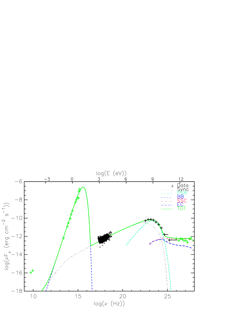
Figure 1.— Phase-averaged broadband SED and an emission model (Section 4.2). Note that X-ray flux varies significantly over the phases, and we show all the X-ray data here. All the Fermi-LAT data points are detected significantly with the TS values greater than 15 and the H.E.S.S. points are denoted in green for better visibility. The model is calculated for 40 phase bins and is averaged. The summed model is shown in solid green, and each component is also shown. Note that we do not attempt to model the low-energy (presumably cooled, large-scale) electron population producing the radio emission. See Section 4.2 and Table 2 for the model and the parameters.

3.2. Fermi-LAT data analysis

We first measure the phase-averaged gamma-ray spectrum of the source using the binned likelihood analysis with the Fermi-LAT gtlike tool. We used a 5^∘ aperture and fit all the bright 3FGL sources (Acero et al., 2015) within the aperture (detected with confidence greater than 5$\sigma$) and the diffuse/isotropic emission (gll_iem_v06; Acero et al., 2016, iso_P8R2_SOURCE_V6_v06). We consider energy dispersion in the analysis. J1018’s emission is modeled with the log-parabola function $dN/dE=N_{\rm 0}(E/E_{\rm b})^{-\alpha-\beta\mathrm{log}(E/E_{\rm b})}$. After this study, we gradually freeze parameters for faint sources until the fit statistic ($k-\mathrm{log}\mathscr{L}$; Akaike, 1974) is minimized in order to remove unnecessary fit parameters. We find that the central values for the best-fit parameters for J1018 do not change in this case, and the best fit is obtained when we fit parameters for five bright sources and the diffuse/isotropic emission. J1018 is detected with high significance (test statistic $TS=14520$) and the new best-fit parameters are very similar to those reported in the 3FGL catalog (Acero et al., 2015). We verified that the results (Table 1) agree with those measured using a large aperture (e.g., $R=15^{\circ}$).

We then estimated systematic uncertainties due to variations of effective area and the interstellar diffuse model (gll_iem_v06). We varied the effective area using the bracketing scales and the normalization of the interstellar diffuse emission by $\pm$6%, and performed gtlike analysis as we did above. The measured SED is shown in Figure 1, and the results of the likelihood fit are presented in Table 1.

Table 1Fit results for the 100 MeV–500 GeV phase-averaged Fermi-LAT data with a log-parabola model

parameter	units	value
$\alpha$	$\cdots$	$2.496\pm 0.013\pm 0.015$
$\beta$	$\cdots$	$0.229\pm 0.009\pm 0.011$
$E_{\rm b}$	GeV	1350.210
$F_{\rm 100\,MeV-500\,GeV}$	$\rm ph\ cm^{-2}\ s^{-1}$	$3.67\pm 0.08\pm 0.12\times 10^{-7}$

^aFixed.
^bStatistical and systematic uncertainties are reported. For the systematic uncertainties, those of the LAT response functions and of the interstellar emission model are summed in quadrature.

We then performed a phase-resolved spectral analysis on 20 orbital phase bins to measure spectral variability of the source. We folded the data on the orbital period ($P_{\rm orb}=16.544$ days) and selected events for each of the 20 phase bins. We performed a binned likelihood analysis using the same parameters for the phase-averaged analysis above, but held all background (diffuse and source) parameters fixed at the phase-averaged values, varying only those for J1018. For each of the 20 phase bins, we generated an SED. These were used to produce energy-resolved orbital light curves (Figure 2). The low-energy $<$400 MeV light curves show structure similar to that seen in the X-ray band; there is a sharp peak at phase 0, and a relatively broad hump at phases 0.2–0.7 (with possibly peaked substructure). At higher LAT energies the broad hump disappears, resulting in a light curve resembling that measured at very high energy (VHE) with H.E.S.S. (Abramowski et al., 2015). We infer that a separate component contributes to the Fermi-LAT band below $\sim$400 MeV.

3.3. Constructing broadband SEDs

We assemble the spectral energy distribution of the source in the radio to the TeV band. The radio, X-ray and TeV data are taken from Ackermann et al. (2012), An et al. (2015), and Abramowski et al. (2015), respectively. We also use the IR-band flux taken from the WISE and the 2MASS catalogs. For the Swift/UVOT data we verified that there is no orbital flux modulation. Therefore, we take the phase-averaged UV flux for the SED. The IR-to-UV magnitudes are properly converted into fluxes and corrected for extinction ($E(B-V)=1.35$; Waisberg & Romani, 2015) with the Schlafly & Finkbeiner (2011) calibration. Note that the IR-to-UV data are well described by a blackbody model having $kT=3.8$ eV and bolometric luminosity $9\times 10^{38}\rm\ erg\ s^{-1}$, typical for an O star (Figure 1). The phase-averaged Fermi-LAT SED was produced as described above (Section 3.2), and we show the broadband SED in Figure 1. Note that the X-ray spectrum varies significantly depending on the orbital phase (An et al., 2013).

In Figure 1, we also show an emission model (see Section 4.2). In this model, X-rays are produced by the synchrotron from shock-accelerated electrons. The H.E.S.S. emission is then produced by external Compton (EC) and synchrotron-self Compton (SSC) up-scattering of the stellar photons and synchrotron photons. In the emission zone, the photon density of the synchrotron emission is $\sim$10 times larger than that of the blackbody emission, which causes SSC to dominate at the highest energies. The Fermi-LAT data are hard to explain with the simple synchro-Compton model. In stochastic shock acceleration theories, the maximum electron energy is limited by the radiation reaction, and the shock accelerated electrons cannot emit synchrotron photons above $\sim$160 MeV. Even with bulk acceleration in the shock (see Section 4), it is hard to explain the full Fermi-LAT data. Furthermore, if the Fermi-LAT photons are produced by the synchrotron process, the light curve should correlate well with the X-ray light curve. However, the high-energy Fermi-LAT light curve does not correlate with the X-ray light curve, hence there must be some other processes responsible for the Fermi-LAT photons. We attribute this to pulsar magnetosphere emission at a few GeV and to EC at the highest energies as we discuss below (Section 4).

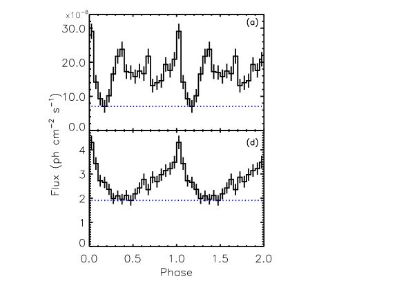
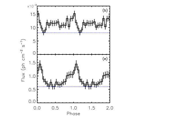
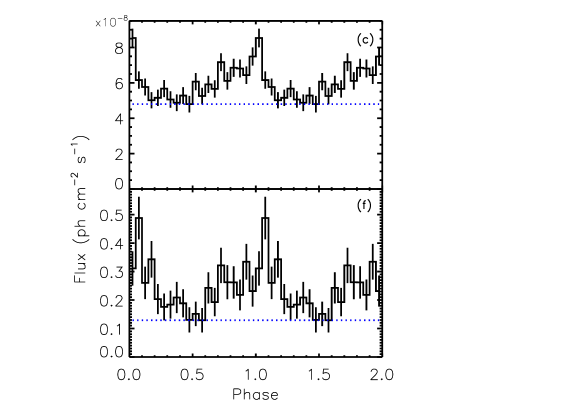
Figure 2.— Energy-resolved Fermi-LAT light curves. Flux is shown as a function of orbital phase. The energy bands are (a) 100–200 MeV, (b) 200–400 MeV, (c) 400-800 MeV, (d) 800–1600 MeV, (e)1600–3200 MeV, and (f) 3200–6400 MeV. The blue line shows the minimum flux level. Note that variability is minimal at intermediate gamma-ray energies. No significant modulation is seen above 6400 MeV due to the paucity of counts.

3.4. Gamma-ray variability

We first checked for secular variation of the gamma-ray flux. This is particularly interesting as the X-ray flux at phase 0 (the spike) is seen to be highly variable, and the other phases are relatively stable. The 3FGL variability index (Acero et al., 2015) is 42, implying no significant phase-averaged variability on a month timescale. Here we investigate variability on shorter time scales, $1-16$ days.

We divided the observation into individual orbits (16.544-day interval). For each time interval, we performed a likelihood fit while holding all the parameters fixed at the mission-averaged values for the corresponding phase (Section 3.2) except for the J1018’s normalization. We measured the source flux for each time interval and constructed the light curve. We then calculated $\chi^{2}$ for a constant flux for the time intervals where the fit successfully converged and the TS value for J1018 is greater than 1. We also varied the model to include other nearby bright sources and/or to let the J1018 spectral shape parameters vary, and find that the best fit was obtained when freeing only the J1018’s normalization. In this case, the $\chi^{2}$/dof for a constant flux is 173.7/142, implying 3% chance that the source flux is constant in time.

We next attempted to study the variability in phase, binning into 1.65-day intervals and then assembling light curves for each of these 10 orbital phase bins. We find no significant ($3\sigma$) flux variability in any phase bins, although the chance probability at phase 9 is relatively low ($p=3$%). Combining phase bins 0 and 9 yields a similar low ($p=3$%) variability significance.

4. Emission modeling

There is growing evidence that the compact object in J1018 is a neutron star, although no study is yet conclusive (Waisberg & Romani, 2015; An et al., 2015; Strader et al., 2015; Williams et al., 2015). Below we model the emission from J1018 under the assumption that the compact object is a neutron star.

If the compact object in J1018 is an energetic spin-powered neutron star, there should be winds from both the neutron star and the optical companion. The two winds form a contact discontinuity (CD) where the ram pressures of the two winds balance. If the stellar wind momentum flux is larger than that of the pulsar wind, the CD curves towards the pulsar. Particles are accelerated to high energy in the shocked pulsar wind. We additionally expect some adiabatic acceleration (e.g., Bogovalov et al., 2008; Dubus et al., 2015) as this shocked wind flows away from the apex along the CD. This is enhanced by the increasingly tangential orientation of the pulsar wind shock as one moves downstream. The net effect is a growing bulk Lorentz factor ($\Gamma$) for the radiating shocked wind. The particles in the shock emit photons via synchrotron and inverse-Compton processes (synchro-Compton model). In this picture the X-ray synchrotron emission is strong at two orbital phases: the periastron and the inferior conjunction of the compact object. This may be able to explain the peculiar X-ray light curve of J1018 (An et al., 2015).

The observed Fermi-LAT light curves (Figure 2) suggest that there should be at least two emission components in that band as noted above (Section 3.2). Furthermore, the substantial steady component in the Fermi-LAT band suggests the existence of an additional “DC” component which we attribute to the pulsar magnetosphere. Keeping these in mind, we model the light curve and the SED of J1018 below.

4.1. Light curve modeling

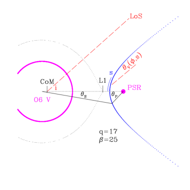
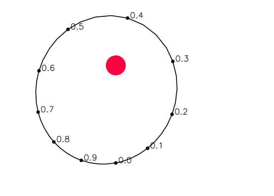
Figure 3.— Left: A vertical cross section of the system. Various geometrical parameters are denoted. Right: A horizontal cross section of the orbit. The position of the neutron star (black dots) in the orbit is shown as a function of orbital phase $\phi_{\rm orb}$. The observer looks at the system from the bottom of the page at an inclination of 50^∘.

We model the X-ray light curve with the synchrotron emission produced by particles flowing along the CD. Near the apex of the CD, the shocked wind has small $\Gamma$ and so emits a nearly isotropic component whose strength varies with the particle and field energy density variations due to the varying IBS standoff distance in the eccentric orbit. The isotropic emission is $F_{\rm iso}\propto B^{2}\propto r_{\rm psr}^{-2}$ (for the assumed synchrotron radiation and a transverse $B$ in a stripped wind), where $r_{\rm psr}$ is the distance from the pulsar to the apex of the CD. The distance is given by the ram pressure balance and is

$$r_{\rm psr}=\frac{a(1-e)}{(1+e\mathrm{\ cos}\phi)}\frac{1}{(1+\sqrt{\eta})},$$

where $a$ is the semi-major axis, $e$ is the eccentricity, $\phi$ is the phase angle (true anomaly), and $\eta$ is the momentum flux ratio of the stellar and pulsar winds. We assume that the masses of the pulsar and the companion are $1.4M_{\odot}$ and $23M_{\odot}$, that the winds of both stars are isotropic and that the wind momentum flux ratio is $\eta=25$. We choose these parameters to be roughly consistent with previous studies (Strader et al., 2015; Dubus, 2006b).

Table 2Parameters used for the light curve and the SED models.

Parameter	Symbol	Value
Eccentricity	$e$	0.35
Inclination (deg.)	$i$	50
Semi-major axis (cm)	$a$	$5.5\times 10^{12}$
Momentum flux ratio	$\eta$	25
Max. bulk Lorentz factor	$\Gamma_{\rm max}$	7
Magnetic field strength (G)	$B$	1.5
Low-energy spectral index	$p_{\rm 1}$	$1.93$
High-energy spectral index	$p_{\rm 2}$	2.15
Minimum electron energy	$\gamma_{\rm e,min}$	$5\times 10^{3}$
Maximum electron energy	$\gamma_{\rm e,max}$	$10^{8}$
Break electron energy	$\gamma_{\rm e,b}$	$5\times 10^{7}$
Injected particle energy ($\rm erg\ s^{-1}$)	$\dot{E}_{\rm P}$	$6\times 10^{35}$
Injected magnetic energy ($\rm erg\ s^{-1}$)	$\dot{E}_{\rm B}$	$3\times 10^{34}$

^aVaries along the shock.

The shape of the CD is calculated following Canto et al. (1996) (see Figure 3 left). Note that, with a synchrotron cooling time $\tau_{c}\approx\frac{3m^{3}c^{5}}{2e^{4}\gamma B^{2}}\approx 5\times 10^{8}\gamma^{-1}B^{-2}$s$\approx 2$s (for Table 2 parameters) shorter than the characteristic flow time along the contact discontinuity $\tau_{f}\approx a/\beta c\approx 40/\beta$s, the high energy electrons can cool in the ‘slow population’, placing a spectral break in the $\sim$MeV range (Figure 1). The lower energy X-ray photons emitted at different distances $s$ along the shock from the apex will have the same spectral slope as that of the isotropically emitted photons near the apex ($\Gamma\approx 1$). Hence Doppler boosting amplification provides the principal variation in emissivity along the shock. Thus for a distance $s$ from the apex where the bulk Lorentz factor has grown to $\Gamma(s)$ the synchrotron emission viewed at angle $\theta_{\rm v}(s)$ is (e.g., see equation 3 of Finke et al., 2008):

$$\mathcal{A}(s)\propto N_{\rm e}(s)\delta_{\rm D}^{(5+p_{\rm 1})/2}(s,\theta_{\rm v})B^{(1+p_{\rm 1})/2}(s),$$

where $N_{\rm e}$ is the number of electrons, $p_{\rm 1}$ is the spectral index of the power-law electron distribution, $\delta_{\rm D}=[\Gamma(1-\sqrt{1-1/\Gamma^{2}}\mathrm{cos}\theta_{\rm v})]^{-1},$ is the Doppler factor, and $B(s)$ is the shock compressed magnetic field strength. Here, we assume that $\Gamma\propto s$, the cumulative shocked plasma $N_{\rm e}\propto 1-\mathrm{cos}\theta_{\rm p}$ where $\theta_{\rm p}$ is the angle between the vector to the emission region from the pulsar and the line of centers, and $B$ is proportional to the distance from the pulsar and the emitting region in the flow ($B\propto r_{\rm p}^{-1}$, where $r_{\rm p}$ is the distance between the pulsar and the emission region).

We are identifying the spike with the Doppler-boosted emission beamed along the IBS. Since this spike is narrow, we require a moderately large $\delta_{\rm D}\stackrel{{\scriptstyle>}}{{{}_{\sim}}}3$. However the spike, while highly variable, is typically only 2–3$\times$ brighter than the phase-averaged flux. Since for $p_{1}\approx 2$ the amplitude scales as $\sim\delta_{\rm D}^{3.5}$, only a small factor ($<10\%$) of the shocked wind can be so highly boosted. Thus we envision two components in the shocked pulsar wind – a low $\sim$constant $\Gamma$ dominant zone that flows along the CD and a higher $\Gamma\propto s$ skin due to adiabatic acceleration and the increasingly tangential nature of the pulsar wind shock. Indeed hydrodynamic simulations (Bogovalov et al., 2008; Dubus et al., 2015) do find such complex post-shock flow patterns.

To summarize, we have a low $\Gamma$ component modulated by the orbital geometry and a higher $\Gamma$ component whose observed intensity is primarily controlled by the line-of-sight beaming angle. The former will be strongest at periastron, which we take to be $\phi_{\rm orb}=0.39$ so that the peak of the model hump coincides with the maximum of the X-ray hump in phase. The latter will be strongest at $\phi_{\rm orb}\approx 0$ generating the spike (see Figure 3 right and Figure 4 top left).

We assume that a broken power-law electron population with a low-energy index of 1.93 so that the model goes through the phase-variable X-ray spectrum (Figure 1), and a high-energy index of 2.15 is injected at the shock (see Section 4.2). Note that the light curve model is insensitive to the exact spectral index. For each phase angle $\phi_{\rm orb}$ in the orbit of the binary, we consider the synchrotron emission of the flows towards the observer at $\phi_{\rm orb}=0^{\circ}$ (corresponding to 201^∘ from the periastron) and inclination $i$ and integrate over the shock surface, covering a range $s=0-3\times$ the orbital separation. We find that this two-component flow explains the X-ray light curve with 3% of the flow in the accelerated component. Figure 4 top left shows the computed X-ray light curve model compared with the data. The eccentricity is constrained by the shape of the sinusoidal hump, and the inclination is by the shape and amplitude of the spike – note in particular that we have chosen $i$ so that the Earth line-of-sight (LoS) is close to grazing incidence for the IBS. At smaller $i$ the spike will be absent and at larger $i$ the spike will be double. The parameters used for the model shown in the figure are $e=0.35$, $i=50^{\circ}$, $B_{\rm apex}=1.5$ G, and maximum $\Gamma=7$ (see Table 2). Note that simple power-law extension of the injection spectrum to lower energies does not alter the fit, hence $\gamma_{\rm e,min}$ is not well constrained.

For the same model we can compute the Sy/EC/SSC components and compare with gamma-ray light curves (Figure 4). At the top right we show the model and data for the low energy Fermi-LAT band. Here synchrotron emission from above the break dominates. For simplicity we have assumed that the injection spectrum does not vary around the orbit and so the shape follows that of the X-ray light curve, with isotropic (hump) and beamed (spike) components. Notice that the rather narrow minimum at $\phi_{\rm orb}\approx 0.2$ and the detailed spiky shape of the hump are not well matched; we comment on this in Section 5. Moving to the $>0.4$ GeV Fermi-LAT band, we are above the spectral cut-off of the unboosted (hump) population. Indeed only the boosted (spike) populations contributes. In both Fermi-LAT panels a phase-independent pulsar contribution (green line) is included. The true amplitude is somewhat uncertain. Moving to the TeV band (bottom right), we expect EC/SSC to dominate. Note that the H.E.S.S. light curve is dominated by the $\phi_{\rm orb}=0$ emission. At first sight this might be surprising, since the EC emission (upscatter of stellar photons) should peak at periastron (broad hump, $\phi_{\rm orb}=0.39$). However, photon-photon absorption (Gould & Schréder, 1967; Dubus, 2006a) by the stellar photons strongly suppresses this component (and the SSC emission from this phase). The absorbed EC and SSC components are shown by the green and blue lines and the total Compton emission shows the phase 0 spike. The slight over-absorption seen at $\phi=0.3-0.5$ may be due to our approximate IBS geometry; some downstream SSC photons can be less strongly absorbed.

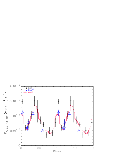
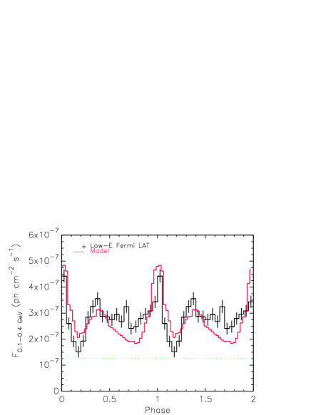
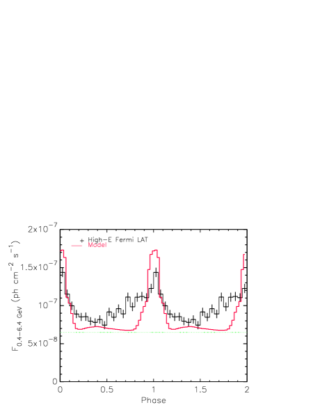
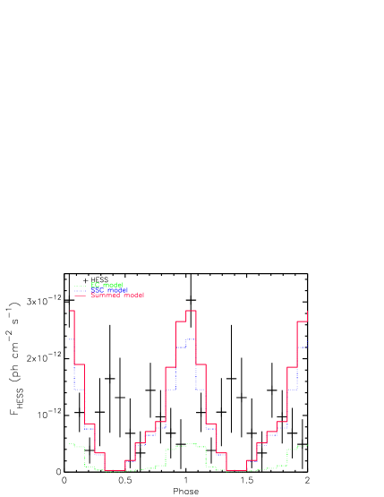
Figure 4.— Top left: The X-ray light curve and a light curve model. The high flare state seen with Swift is not shown in this plot. Top right: Low-energy (100–400 MeV) Fermi-LAT light curve and a light curve model. Bottom left: High-energy (0.4–6.4 GeV) Fermi-LAT light curve and a light curve model. The green line in the top-right and bottom-left panels shows the pulsar contribution. Bottom right: The H.E.S.S. light curve and a light curve model. The H.E.S.S. data of Abramowski et al. (2015) is newly folded at the X-ray orbital period used in this paper (de Oña-Wilhelmi, private communication). The parameters for the model are $i=50^{\circ}$, $P_{*}c/E_{\rm psr}=25$, and $\Gamma_{\rm max}=7$ (see Section 3.2).

4.2. Phase-resolved SED model

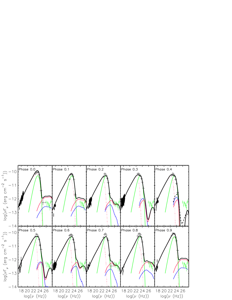
Figure 5.— Phase-resolved broadband SEDs and the emission model (Section 4.2). The X-ray-to-Fermi-LAT data are phase-resolved (black crosses), and phase-averaged H.E.S.S. data (green crosses; Abramowski et al., 2015) are also shown for reference. The model is calculated for 40 phase bins and re-summed to the 10 panels shown. Lines are for model components: synchrotron (red dotted), pulsar (green), SSC (red solid), EC (blue solid), and the sum (black solid). Photon-photon absorption is calculated assuming that emission is all from the apex of the shock. However, for phase 0.4, we also show the high-energy SED with photon-photon absorption calculated using the realistic shock geometry (black dot-dashed line). See Section 4.2 and Table 2 for the model and the parameters. Notice that the synchrotron emission goes up to the highest frequency at phase 0 as expected due to the high bulk Lorentz factor.

We model the SED with a synchro-Compton model with an addition of a pulsar magnetosphere component. This pulsar emission is a power law with sub-exponential cutoff, $dN/dE=N_{\rm 0}(E/E_{\rm 0})^{-\Gamma_{\rm psr}}{\rm exp}[-(E/E_{\rm c})^{b}]$, where we used $N_{\rm 0}=5.7\times 10^{-7}\rm\ ph\ cm^{-2}\ s^{-1}\ GeV^{-1}$, $E_{\rm 0}=1$ GeV, $\Gamma_{\rm psr}=0.7$, $E_{\rm c}=110$ MeV, and $b=0.48$, corresponding to $L_{\gamma}\simeq 5\times 10^{35}\rm\ erg\ s^{-1}$ for an assumed distance of 5 kpc to match the observed Fermi-LAT SED. Note that these pulsar parameters are typical for gamma-ray pulsars with sub-exponential cutoff spectra (Abdo et al., 2013). The star emits blackbody photons with $kT\sim 4$ eV and $L_{\rm BB}=10^{39}\ \rm erg\ s^{-1}$ and provides seed photons for EC scattering, and absorbs the TeV emission.

We use the same parameters that we used for the X-ray light curve modeling (see Section 4.1) and compute the EC and SSC emission. Note that we use a broken power-law electron distribution. A broken power-law distribution can be formed due to particle cooling (e.g., Moderski et al., 2005). In our case, electrons are injected by the pulsar over the whole shock. Those injected near the apex flow and cool along the shock. Therefore, at any point in the shock, there are cooled electrons and freshly injected electrons. This process necessarily produces a broken power-law distribution. Note that the break $p_{\rm 2}-p_{\rm 1}$ is not 1 in our case; a break of 1 is expected for electrons cooling in homogeneous magnetic field. In our model, the magnetic field strength decreases with distance ($s$), hence the break may be smaller.

We adjust the maximum electron Lorentz factor ($\gamma_{\rm e,max}$) at each point of the shock so that the maximum synchrotron frequency in the rest frame of the flow is $\sim$160 MeV, the radiation reaction limit. The spectral break energy evolution is calculated by integrating $\dot{\gamma}\propto-B^{2}\gamma^{2}$, assuming synchrotron cooling dominates. We also compute the gamma-gamma absorption between the high-energy EC/SSC photons and the stellar photons (see, for example, Dubus, 2006a). For this, we assumed that the optical star is a point source and all the high-energy TeV photons are emitted at the apex of the shock for simplicity. We calculate the differential optical depth given in Dubus (2006a) at each point along the LoS and integrate it out to $\sim$10$\times$ the distance between the star and the emitting region. Beyond this distance, the blackbody photon field becomes negligibly weak, as does the absorption. The absorption is then computed by taking the exponential of the integrated optical depth.

Note that here we calculated the effect of absorption only for spectrum emitted at the apex of the shock in each phase and assumed that this is the same for emission over the whole shock. The absorption is strongest at phase $\sim$0.4 (when the compact object is behind the optical companion) and at $\sim 10^{25}$ Hz. Hence the effect of the absorption is to remove the sinusoidal hump in the (low-energy) H.E.S.S. light curve. We calculate the model emission for 40 phase bins and show the phase-averaged SED and the model in Figure 1. We note that the model also explains the phase-resolved SEDs reasonably well (Figure 5).

The maximum photon frequency of the synchrotron emission is highest at phase 0 because of Doppler boosting. Hence, a significant amount of high-energy synchrotron photons ($\stackrel{{\scriptstyle>}}{{{}_{\sim}}}1$ GeV) is produced only near phase 0, and the pulsar emission dominates the GeV band in the other phases. Photons in the sinusoidally modulating phases extend only up to $\sim 200$ MeV (no Doppler boosting), hence are visible only in the lower-energy Fermi-LAT light curve. Therefore, the low-energy Fermi-LAT light curve shows two peaks while the high-energy one has only one (Figure 4).

5. Discussion and Conclusions

Gamma-ray binaries such as LS 5039 show only broad variation in the TeV band, which is interpreted as orbital modulation of EC emission. J1018 uniquely shows two components in the Fermi-LAT band, a broad modulation and a sharp spike; the spike continues into the TeV range. Moreover the finding of Strader et al. (2015) that the spike phase corresponds to compact object (neutron star) inferior conjunction argues against a simple EC interpretation. We have shown that this multi-component picture can be understood by positing slow and faster (moderate $\Gamma$) flow in a shocked pulsar wind. Both components contribute synchrotron emission in the X-ray to the low-energy Fermi-LAT band; only the Doppler boosted component reaches energies above 1 GeV. The broad hump (low $\Gamma$) emission is very asymmetric. In our model, this is explained by orbital eccentricity ($e\sim 0.35$).

The spike emission depends on Doppler boosting and thus places significant constraints on the $\Gamma$ and viewing geometry. Existence of such beamed emission in gamma-ray binaries has been suggested (e.g., Dubus et al., 2015; Dubus, 2015), and similar phenomena have been seen in some pulsar binaries (e.g., Romani & Sanchez, 2016) as well. Modeling the spike allows us to infer the properties of the fast flow and the orbital parameters; the maximum bulk Lorentz factor of the flow is $\sim$7 and the inclination is $\sim$50^∘ (for $\eta=25$). This inclination is in agreement with estimates obtained by spectroscopic study ($32^{\circ}-49^{\circ}$ for $M_{*}=20M_{\odot}$ or $39^{\circ}-64^{\circ}$ for $M_{*}=26.4M_{\odot}$; Strader et al., 2015). It should be noted that the required inclination is somewhat dependent on the momentum flux ratio $\eta$ assumed here, and might be somewhat different in a detailed hydrodynamic simulation (e.g., Bogovalov et al., 2008).

Our interpretation on the X-ray spike enables several specific predictions. First, because the beamed emission is produced by synchrotron radiation of cooled electrons, the spectrum should have a different spectral break at different phases. While we expect that the actual break energy is inaccessible at $\sim$MeV energies, precision X-ray phase spectra might be compared with phase-resolved Fermi-LAT spectra at low energies to reveal break shifts. Also, the X-ray flux variability of the spike is expected because a small change of the beaming angle (shape of the CD) due to the variation of stellar wind momentum flux can result in a large change in the flux. Our current constraint on the inclination is such that the observer sees the shock slightly above the asymptotic tangent of the shock. Larger stellar winds will make the opening angle of the shock smaller and the synchrotron flux will drop. In principle a large drop in the stellar wind flux might allow the IBS to expand sufficiently to show a broader or even doubled peak bracketing phase 0. This can be tested with optical/X-ray monitoring to infer $\eta$ variations.

The change of the light-curve shape in the Fermi-LAT band suggests another constant emission component in that band. We assume that this component is the pulsar magnetosphere emission. Alternatively, it could be EC up-scattering of the stellar photons by a lower-energy relativistic Maxwellian distribution as hypothesized by Dubus et al. (2015). If so, this component will produce a broad hump peaking at the periastron in the light curve. Perhaps, some of the low-energy Fermi-LAT flux may be attributed to this. Whether or not this can explain the constant flux is unclear. Nevertheless, if our interpretation of the Fermi-LAT-band emission is correct (i.e., the pulsar contributes significantly), it may be possible to detect gamma-ray pulsations when the orbital parameters are better constrained.

Our model captures the main features of the Fermi-LAT light curves (Figure 4). In particular, boosted synchrotron emission accounts for the spike at phase 0 and contributes to the bump at phase 0.3–0.4. However, the bump is too weak and we overproduce the emission at phase 0.1–0.2. We cannot attribute the dip at this phase to absorption since the pulsar is in front. Thus we infer a somewhat lower pulsar contribution at these energies and a larger modulation of the synchrotron shock flux.

A possible source of such modulation is asymmetry in the pulsar wind; many young pulsars have wind nebulae concentrated in an equatorial torus. If such a torus is inclined with respect to the orbital plane then the two cross at two phases. Thus we can imagine the pulsar wind pole pointing to phase $\phi\sim 0.1-0.2$ with a weaker shock and decreased synchrotron emission, while the equatorial flow at phase $\phi\sim 0.35-0.5$ might give rise to enhanced emission, near periastron. At phase 0.8–0.9 the wind interaction would be weakened by the larger orbital separation. Note that the enhanced synchrotron emission could add additional SSC flux at $\phi\sim 0.35-0.5$, where the H.E.S.S. data also lie above the model. Modeling such an anisotropic wind lies beyond the scope of this paper.

In the TeV band we see boosted SSC at the phase 0 spike. This appears especially sharp in the refolded H.E.S.S. data and so some amendments to the model (e.g. sharper shock spatial curvature due to an anisotropic pulsar wind and/or higher bulk $\Gamma_{\rm max}$) might be useful.

We can also expect additional SCC modulation if the pulsar wind is anisotropic. We generally expect a broad sinusoidal hump from EC emission in the $\sim 10$ GeV–TeV band. However in our model absorption from the soft stellar photons nearly completely suppress this component (Figure 5). Our model computes a simple exponential attenuation of the shock flux, assuming that the emission is located near the apex and integrating the optical depth of the stellar photon field along the instantaneous line of sight. This is almost certainly an over-estimate.

To test this, for phase 0.4 we recomputed the absorption by computing the optical depth for each emission point along the shock surface. As the distance $s$ from the apex increases, absorption decreases for that portion of the shock above the orbital plane and increases for the part of the shock that lies below. Given the exponential nature of the attenuation, the effect on the total emission integrated over the entire surface is a decreased absorption, up to $6\times$ less than in the point source approximation. This estimate is shown as the dashed line in Figure 5. The details of this absorption depend on the detailed shock structure (e.g. modified by anisotropic pulsar emission), so further analysis can await more detailed observation.

A second effect can also boost the observed TeV flux at these phases: secondary $e^{+}/e^{-}$ pairs produced in TeV absorption on stellar photons can emit in the $\sim 10^{24}-10^{25}$ Hz band (e.g., Bednarek, 2013; Dubus, 2013). This cascade emission can be especially important near pulsar superior conjunction and so may also contribute to the lower energy TeV emission at $\phi\sim 0.3-0.5$. TeV phase-resolved spectra anticipated in the Cherenkov Telescope Array (CTA) era would certainly motivate such detailed modeling of the absorption and re-emission.

In addition to reproducing the multiband light curves fairly well, our model can match the phase-resolved SEDs (Figure 5). The gamma-ray luminosity of the putative pulsar is $\sim$$10^{36}\rm\ erg\ s^{-1}$. This suggests a very energetic young pulsar (consistent with the young massive binary). Comparing with Abdo et al. (2013) suggests a parent pulsar with $\mathrm{Log}({\dot{E}})\approx 36-39$, which could certainly supply the required particles and magnetic energy for the shock (Table 2). A gamma-ray pulse detection would be a crucial input to a more detailed model.

The H.E.S.S. spectrum appears to rise above 10 TeV. This is not a feature of our current SED, but could be easily accommodated if we introduced low-energy seed photons ($\nu\stackrel{{\scriptstyle<}}{{{}_{\sim}}}10^{12}-10^{13}$ Hz) and maintained a hard $e^{+}/e^{-}$ injection. While radio-millimeter observations can probe this population, it may be difficult to compute the $\stackrel{{\scriptstyle>}}{{{}_{\sim}}}$10 TeV spectrum since Compton-upscattering of these soft photons depends on the poorly known scattering geometry. Much of the population of these slow-cooling electrons may be at large $s$ and less useful for Compton upscatter. An inner-system low-energy synchrotron component however might be due to low-energy pulsar injection as hypothesized by Dubus et al. (2015). Another possible contribution to the TeV flux might be traced to the very hard (albeit with large uncertainty) X-ray spectra seen by An et al. (2013) at several phases. These data may require the injection spectrum to vary with orbital phase. This could be another signature of an anisotropic pulsar wind and we would benefit from better constraints on the X-ray spectrum phase variation. Detailed phase information on the $\stackrel{{\scriptstyle>}}{{{}_{\sim}}}$10 TeV flux would also be quite helpful – and should be available in the CTA era.

We conclude that 1FGL J1018.6$-$5856 can provide a good opportunity to study shock acceleration and hydrodynamic flow in gamma-ray binaries thanks to its peculiar X-ray-to-gamma-ray light curves, with multiple emission components appearing in the several wavebands. While our observationally driven model reproduces important features of the light curves and SEDs, detailed relativistic hydrodynamic simulations and monitoring observations may well be needed for a full understanding. As a test case with particularly rich behavior, J1018 can certainly give us new insights into IBS emission in gamma-ray binaries.

We thank E. de Oña Wilhelmi and the H.E.S.S. collaboration for providing the H.E.S.S. light curve folded on the refined orbital period. The Fermi LAT Collaboration acknowledges generous ongoing support from a number of agencies and institutes that have supported both the development and the operation of the LAT as well as scientific data analysis. These include the National Aeronautics and Space Administration and the Department of Energy in the United States, the Commissariat à l’Energie Atomique and the Centre National de la Recherche Scientifique / Institut National de Physique Nucléaire et de Physique des Particules in France, the Agenzia Spaziale Italiana and the Istituto Nazionale di Fisica Nucleare in Italy, the Ministry of Education, Culture, Sports, Science and Technology (MEXT), High Energy Accelerator Research Organization (KEK) and Japan Aerospace Exploration Agency (JAXA) in Japan, and the K. A. Wallenberg Foundation, the Swedish Research Council and the Swedish National Space Board in Sweden.

Additional support for science analysis during the operations phase is gratefully acknowledged from the Istituto Nazionale di Astrofisica in Italy and the Centre National d’Études Spatiales in France.

H.A. acknowledges supports provided by the NASA sponsored Fermi Contract NAS5-00147 and by Kavli Institute for Particle Astrophysics and Cosmology (KIPAC). This work was supported by the research grant of the Chungbuk National University in 2016.

References

- Abdo et al. (2013) Abdo, A. A., Ajello, M., Allafort, A., et al. 2013, ApJS, 208, 17
- Abramowski et al. (2015) Abramowski, A., Aharonian, F., Ait Benkhali, F., et al. 2015, A&A, 577, A131
- Acero et al. (2015) Acero, F., Ackermann, M., Ajello, M., et al. 2015, ApJS, 218, 23
- Acero et al. (2016) —. 2016, ApJS, 223, 26
- Ackermann et al. (2012) Ackermann, M., Ajello, M., Ballet, J., et al. 2012, Science, 335, 189
- Akaike (1974) Akaike, H. 1974, IEEE Transactions on Automatic Control, 19, 716
- An et al. (2013) An, H., Dufour, F., Kaspi, V. M., & Harrison, F. A. 2013, ApJ, 775, 135
- An et al. (2015) An, H., Bellm, E., Bhalerao, V., et al. 2015, ApJ, 806, 166
- Atwood et al. (2013) Atwood, W., Albert, A., Baldini, L., et al. 2013, ArXiv e-prints, arXiv:1303.3514
- Bednarek (2013) Bednarek, W. 2013, Astroparticle Physics, 43, 81
- Bogovalov et al. (2008) Bogovalov, S. V., Khangulyan, D. V., Koldoba, A. V., Ustyugova, G. V., & Aharonian, F. A. 2008, MNRAS, 387, 63
- Bosch-Ramon & Paredes (2004) Bosch-Ramon, V., & Paredes, J. M. 2004, A&A, 417, 1075
- Canto et al. (1996) Canto, J., Raga, A. C., & Wilkin, F. P. 1996, ApJ, 469, 729
- Coley et al. (2014) Coley, J. B., Corbet, R., Cheung, C. C., et al. 2014, in AAS/High Energy Astrophysics Division, Vol. 14, AAS/High Energy Astrophysics Division, 122.10
- Dubus (2006a) Dubus, G. 2006a, A&A, 451, 9
- Dubus (2006b) —. 2006b, A&A, 456, 801
- Dubus (2013) —. 2013, A&A Rev., 21, 64
- Dubus (2015) —. 2015, Comptes Rendus Physique, 16, 661
- Dubus et al. (2015) Dubus, G., Lamberts, A., & Fromang, S. 2015, A&A, 581, A27
- Finke et al. (2008) Finke, J. D., Dermer, C. D., & Böttcher, M. 2008, ApJ, 686, 181
- Gould & Schréder (1967) Gould, R. J., & Schréder, G. P. 1967, Physical Review, 155, 1404
- Johnston et al. (1992) Johnston, S., Manchester, R. N., Lyne, A. G., et al. 1992, ApJ, 387, L37
- Leahy (1987) Leahy, D. A. 1987, A&A, 180, 275
- Mirabel (2012) Mirabel, I. F. 2012, Science, 335, 175
- Moderski et al. (2005) Moderski, R., Sikora, M., Coppi, P. S., & Aharonian, F. 2005, MNRAS, 363, 954
- Poole et al. (2008) Poole, T. S., Breeveld, A. A., Page, M. J., et al. 2008, MNRAS, 383, 627
- Romani & Sanchez (2016) Romani, R. W., & Sanchez, N. 2016, ApJ, 828, 7
- Schlafly & Finkbeiner (2011) Schlafly, E. F., & Finkbeiner, D. P. 2011, ApJ, 737, 103
- Strader et al. (2015) Strader, J., Chomiuk, L., Cheung, C. C., Salinas, R., & Peacock, M. 2015, ApJ, 813, L26
- Tavani et al. (1994) Tavani, M., Arons, J., & Kaspi, V. M. 1994, ApJ, 433, L37
- Waisberg & Romani (2015) Waisberg, I. R., & Romani, R. W. 2015, ApJ, 805, 18
- Williams et al. (2015) Williams, B. J., Rangelov, B., Kargaltsev, O., & Pavlov, G. G. 2015, ApJ, 808, L19