Optimal control of eye-movements during visual search

Abstract

We study the problem of an optimal oculomotor control during the execution of visual search tasks. We introduce a computational model of human eye movements, which takes into account various constraints of the human visual and oculomotor systems. In the model, the choice of the subsequent fixation location is posed as a problem of a stochastic optimal control, which relies on reinforcement learning methods. We show that if biological constraints are taken into account, the trajectories simulated under a learned policy share both basic statistical properties and a scaling behaviour with human eye movements. We validated our model simulations with human psychophysical eye-tracking experiments.

1 Introduction

The human oculomotor system performs hundreds of thousands of eye-movements per day during the execution of different behavioral tasks. In order to find the details of a visual scene related to the tasks, humans direct foveal vision to the most informative locations via saccades - high-velocity conjugate gaze shifts. Saccades are followed by a visual fixation, during which the human oculomotor system generates fixational eye movements involuntarily. Despite the remarkable achievements in the modelling of fixational eye movements and the interpretation of their fundamental properties [1, 2, 3], there is no comprehensive generic model of fixation selection [4, 5, 6], which takes into account the underlying mechanisms of visual attention [5, 7, 8] and qualitatively describes the statistical properties of saccadic eye-movements during the execution of visual tasks [9, 10, 11, 12].

Previously, the problem of fixation selection was studied in the framework of control models of eye movements [13, 11, 9]. In control models the observer gathers information about the world during each fixation, integrates information over all fixations into a belief state and makes a choice of the next location on which to fixate. This choice is governed by the policy of gaze allocation - a function that specifies the action of decision-maker in a certain belief state. It was shown that the policy based on information maximization criteria [9] generates trajectories that share basic statistical properties with human eye movements. In this research, we set the goal of developing a control model of fixation selection that is capable of interpreting the scaling behaviour of human eye-movements [10, 14, 12, 15] and provides a human level of performance to a computational agent.

In contrast to the previous research on control models, we take into account the inherent uncertainty of human oculomotor system and the duration of saccadic eye movements. It’s well known that any motor action of humans is executed with random error, which increases with movement magnitude [16, 17]. Despite the oculomotor system having developed a correction mechanism for saccade errors [18], these result in inevitable temporal costs. Furthermore, the duration of saccades is empirically correlated with their magnitude as well [19]. These factors result in situations where the observer has to choose between more informative remote (and riskier) locations and those nearby (but less informative ones). We show that if these constraints are taken into consideration, the trajectories simulated under a learned policy share both basic statistical properties and scaling behavior with human eye movements, which is not achievable with the conventional infomax model [9].

On the basis of our results, we argue that we have made the following contribution:

• The formulation of the biologically plausible model of gaze allocation in the human observer from the point of view of stochastic optimal control. The representation of the model in the form of partially observable Markov decision process (PO-MDP) and the proposal of a heuristic policy.

• The development of robust and high performance algorithms of simulation of PO-MDP. The implementation of reinforcement learning algorithms of policy optimization and numerical estimation of the optimal policy of gaze allocation.

• The comprehensive statistical analysis of simulated trajectories and data from our psycho-physical experiments. The policy, which is learned with the policy gradient REINFORCE algorithm, shows the highest level of statistical similarity with human eye-movements. In our experiments we discovered the dependency of the mean saccade length and q-order Hurst exponent on visibility of the target, which was explained by our model.

2 Model of the ideal observer

In this section we formulate the model of the ideal observer, which aims to localize the single target object on the stationary 2D image. We represent the model in the form of partially observable Markov decision process (PO-MDP), which is summarized by flow chart on Figure 1.

Figure 1: Flow chart of the model of the ideal observer. The visual search is a recurrent process that starts after initialization of the world state. On each consequent step the observer receives the observation vector $\mathbf{W}_{n}$, which is then used for estimation of belief state $p_{n}$ using Bayesian inference [20]. After the update of the belief state the observer makes the decision $D_{n}$ where to fixate next according to the policy of gaze allocation: $D_{n}=\mu(p_{n})$. The next fixation location is defined by execution function: $A_{n+1}=\alpha(D_{n})$. If the observer fixates on the location of target $A_{n+1}=m$ the process of visual search is terminated, otherwise the next step starts with updated values of variables.

2.1 World state

At the beginning of each episode the target object appears randomly at one of $L$ possible locations. We assume that the target is placed on background noise or surrounded by distractors, which are placed on vacant locations. The world state $S_{n}$ is represented as a tuple:

$$S_{n}=\left(m,\ A_{n},\ t_{n}\right)$$ (1)

where $m$ is a location of the target on the image and $A_{n}$ is gaze fixation location that changes with the number of step $n$, and $t_{n}$ is time passed from the start of a trial and the step $n$.

If the observer fixates the gaze on the location of target:

$$A_{n}=m$$ (2)

the visual task is considered to be accomplished. This formulation of the terminal state reflects the necessity to foveate the target in order to extract as much information about its identity and details as possible. The location of target $m$ doesn’t change during a trial.

2.2 Update of belief state

The decision-making of the observer is modeled as PO-MDP with a belief state $p_{n}$ - a discreet probability distribution function of target location given all observations received up to the step $n$. Because the observer is instructed that the target appears randomly, the initial belief state $p_{0}$ is a discrete uniform distribution.

On each step $n$ observer receives the observation vector $\mathbf{W}_{n}=\left(W_{1,n},\ldots,W_{L,n}\right)$, whose elements represent the perceptual evidence that the target is at corresponding locations. The probability distribution function is updated using Bayesian inference [20]:

$$\mathrm{\mathit{p_{n}(l)=\frac{p_{n-1}(l)p(\mathbf{W}_{n}|l,A_{n})}{\underset{k}{\sum}p_{n-1}(k)p(\mathbf{W}_{n}|k,A_{n})}}}$$ (3)

where $l$ is the index of the location and $p(\mathbf{W}|l,A)$ is an observation model. In order to take into account the uncertainty of the processing of perceptual information within the neural circuits of the observer, we follow the “noisy observation” paradigm [9]. In this paradigm the observation model $p(\mathbf{W}|l,A)$ reflects the presence of the observer’s internal sources of inefficiency, such as physical neural noise on all stages of information processing. According to the perceptual model [11] the observation $\mathbf{W}$ may be represented as a random variable with Gaussian distribution with mean depending on the location $m$ of the center of target on the lattice:

$$p(\mathbf{W}|l,A)=\underset{l}{\prod}p(W_{l}|A) =$$

$$\underset{l}{\prod}N\Bigl{(}W_{l};\delta_{l,m}^{\mathbf{}},\frac{1}{F\left(\left\|l-A\right\|\right)}\Bigr{)}$$ (4)

where $\delta_{i,j}^{\mathbf{}}$ is Kronecker delta, $N(x,\mu,\nu)$ is a value of Gaussian function with mean $\mu$ and variance $\nu$ for argument $x$; $\left\|l-A\right\|$ is Euclidean distance between the locations $l$ and the current fixation $A$, and $F$ is a Fovea-Peripheral Operating Characteristic (FPOC) [13]. FPOC is a function that represents the dependence of a signal-to-noise ratio on the eccentricity. Figure 2 demonstrates FPOC calculated for several values of RMS contrast of the background 1/f noise: $e_{n}\in\left(0.1,0.15,0.2,0.25\right)$ and a single value of RMS contrast of target $e_{t}=0.2$. The calculation are based on the analytical expressions from [11]. The signal-to-noise ratio has a peak at fovea and decreases rapidly with eccentricity.

In our simulations we consider only the case of the rotationally symmetric FPOC. This assumption is not correct for human observers, and better generic model of FPOC can be found in [21]. The broken circular symmetry of FPOC inevitably results in the asymmetry of the visual search process [22]. We simplify the model of FPOC, because in this research we focus our attention more on the temporal structure of eye-movements rather than on their spatial distribution.

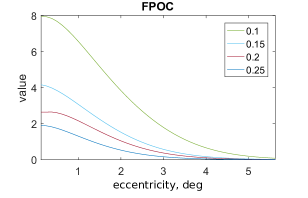
Figure 2: Fovea-Peripheral Operating Characteristic was calculated for several values of the RMS contrast of background noise: $e_{n}\in\left(0.1,0.15,0.2,0.25\right)$ and the single value of RMS contrast of target $e_{t}=0.2$. The signal-to-noise ratio has a peak at fovea and decreases rapidly with eccentricity.

2.3 Execution of saccades

The decision of which location to fixate next, $D_{n}$, is made on each step of PO-MDP according to the policy of gaze allocation $\mu:$

$$D_{n}=\mu(p_{n})$$ (5)

After making the decision, the coordinates of the next fixation location $A_{n+1}$ are defined by the execution function:

$$A_{n+1}=\alpha(D_{n})=D_{n}+J_{n}$$ (6)

where $J_{n}$ is a Gaussian-distributed random error with zero mean and standard deviation $\nu$ defined in [17]:

$$\nu=\zeta_{0}+\zeta_{1}\left\|D_{n}-A_{n}\right\|$$ (7)

The error of the saccade execution is proportional to intended saccade amplitude $\left\|D_{n}-A_{n}\right\|$ given in degrees, the value of parameters: $\zeta_{0}=0.87\deg$, $\zeta_{1}=0.084$ (from[17]).

The next step of PO-MDP starts after the transition to the location $A_{n+1}$. This decision-making model may be easily extended in order to take into account the extraction of visual information between the moment of making the decision where to fixate next and completion of the saccade.

2.4 Duration of the steps

After each consequent step the time variable $t$ of world state (1) is updated in a deterministic way:

$$t_{n}=t_{n-1}+\Theta(n)$$ (8)

where $\Theta(n)$ is a duration of step $n$. The duration of time step $\varTheta(n)$ is considered as a total time, which is required for the relocation of the gaze from a previous location $A(n-1)$ to the current one $A(n)$ and the extraction of visual information from the location $A(n)$. Therefore, we consider $\varTheta(n)$ as a sum of durations of the fixation $\varTheta_{fix}(n)$ and the saccade $\varTheta_{sac}(n)$. According to the literature, both of these time intervals are empirically correlated with a magnitude of the saccade preceding the fixation [19, 23, 24]. The duration of saccadic eye-movements $\varTheta_{sac}(n)$ in range of magnitudes from $1.5\textdegree$ to $30\textdegree$ is possible to approximate as [25]:

$$\varTheta_{sac}(n)=\tau_{sac}\left\|A_{n}-A_{n-1}\right\|^{0.4}$$ (9)

where $\tau_{sac}=21ms\cdot\deg^{-0.4}$. Besides the magnitude of saccade, the fixation duration $\varTheta_{fix}(n)$ is influenced by various factors as a discriminability of the target [26], its complexity and the visual task of the observer [24, 27]. However, if the observer is correctly informed about the targets’ properties before the task execution and performs the visual task without any interruptions, the contribution of these factors to the fixation duration (with exception of magnitude) is constant during each trial. The eye-tracking experiments with the fixations tasks [23, 24, 28] found that the dependence of fixation duration on saccade amplitude is linear:

$$\varTheta_{fix}(n)=\left\|A_{n}-A_{n-1}\right\|\tau_{fix}+\varTheta_{0,fix}$$ (10)

with a slope $\tau_{fix}=6ms/\deg$. The constant $\varTheta_{0,fix}=250ms$ is an intercept, averaged from values from eye-tracking data [29, 30]. Finally, the duration of step $n$ is:

$$\varTheta(n)=\varTheta_{sac}(n)+\varTheta_{fix}(n)$$ (11)

The values of parameters used in simulations are consistent with our estimates from the eye-tracking experiments: $\tau^{*}_{sac}=20\pm 3ms\cdot\deg^{-0.4}$, $\tau^{*}_{fix}=5.8\pm 1.8ms/\deg$, $\varTheta_{0,fix}=241\pm 42ms$. Within this range of the parameters’ values we didn’t find a substantial difference in the estimates of the learned policy of gaze allocation.

2.5 Value function

Given the initial world state $S_{0}$, we define the cost function for policy $\mu$ as an expectation of a random variable $V$:

$$V_{\mu}(S_{0})=E\left[V|\mu,S_{0}\right]$$ (12)

The random variable $V$ denotes the cost and is defined by:

$$V\equiv c\sum_{n=0}^{N}\varTheta(n)=ct_{N}$$ (13)

where $N$ is a total number of steps in the episode, and $c$ is a time cost constant.

Formulation of the cost function in a real time sets this study separately from the previous works [31, 11, 13]. We show below, that the policy $\mu$ optimized for the cost function with the reward defined in (13) generates the sequences of actions with statistical characteristics close to the human saccadic eye-movements.

3 Policy of gaze allocation

3.1 Infomax approach

In this section we describe two heuristic policies related to the model of Entropy Limit Minimization searcher [9]. We define the information gain on the step $n+1$ as: $\triangle I(n+1)=H(p_{n})-H(p_{n+1})$, where $H\left(\cdot\right)$ is Shannon entropy. The heuristic policy $\pi_{0}$ is defined as a policy which chooses such decision $D_{n}$ that maximizes the expected information gain $\triangle I(n+1)$:

$$\pi_{0}(p_{n})=D_{n}=\underset{D}{\arg\max}\left[E\left[\triangle I(n+1)\right]\right]$$ (14)

The term $E\left[\triangle I(n+1)\right]$ is calculated analytically in [9] for the case of the saccadic eye-movements without uncertainty ($A_{n+1}\equiv D_{n})$:

$$E\left[\triangle I(n+1)\right]=\frac{1}{2}\left(p_{n}*F^{2}\right)\left(D_{n}\right)$$ (15)

where sign $*$ denotes a convolution operator, and $F$ is FPOC represented as a radially symmetric 2D function: $F(A)\equiv F\left(\left\|A\right\|\right)$. The expression (15) gives an approximate value of the expected information gain in the case of the stochastic saccadic placement (6).

The figure 3 illustrates the decision-making process, which corresponds to the policy $\pi_{0}$. The colour map (left) represents the function of the expected information gain (equation (15)). The blue cross corresponds to the location of the current fixation on the step $n$. The observer makes a decision to fixate at the location defined by the policy: $D_{n}=\pi_{0}(p_{n})$. This decision results in a saccadic eye-movements to location $A_{n+1}=\alpha(D_{n})$ marked by the green cross. After receiving the observation at the step $n+1$, the observer updates the belief state and evaluate the information gain for the next decision. In this particular situation, the target was absent at the vicinity of $A_{n+1}$, and the observation resulted in the decline of probability $p_{n+1}$ in the area around the green cross (figure 3 right). This area is effectively inhibited from subsequent fixations due to low probability. The size of this area is defined by values of FPOC ($e_{t}=0.2$, $e_{n}=0.1$ in this case). We call the policy $\pi_{0}$ “infomax greedy” in the text below.

The trajectories generated with infomax greedy policy match the basic properties of human eye movements [9]. However, the policy (15) doesn’t consider the correlation between the magnitude of saccades and the durations of steps of MDP. We show later that the policy $\pi_{0}$ is inferior to the policy that optimizes the expected rate of information gain $E\left[\triangle I(n+1)/\varTheta(n+1)\right]$:

$$\pi_{1}(p_{n})=\underset{D}{\arg\max}\left[E\left[\triangle I(n+1)/\varTheta(n+1)\right]\right]$$ (16)

Using the expression for $E[\triangle I(n+1)]$ (15), for the deterministic saccadic placement $(A_{n+1}\equiv D_{n})$:

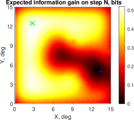
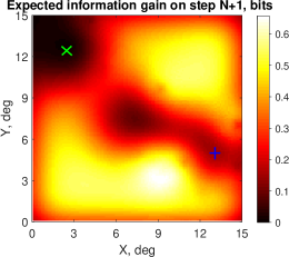
Figure 3: The decision-making process under the infomax greedy policy $\pi_{0}$ [9]. The colour map (left) represents the function of the expected information gain (equation (15)). The blue cross corresponds to location of the current fixation on the step $n$. The observer makes a decision to fixate at the location defined by the policy: $D_{n}=\pi_{0}(p_{n})$. This decision results in the saccadic eye-movement to location $A_{n+1}=\alpha(D_{n})$ marked by the green cross. After receiving the observation at the step $n+1$, observer updates the belief state and evaluates the information gain for the next decision. In this particular situation, the target is absent in the vicinity of $A_{n+1}$, and the observation resulted in the decline of probability $p_{n+1}$ in the area around the fixation (the green cross). This area is effectively inhibited from the subsequent fixations due to low probability $p_{n+1}$. The size of this area is defined by the values of FPOC (in this case $e_{t}=0.2$, $e_{n}=0.1$).

$$\pi_{1}(p_{n})=D_{n}=\underset{D}{\arg\max}\left[\frac{\left(p_{n}*F^{2}\right)\left(D_{n}\right)}{\varTheta(n+1)}\right]$$ (17)

The policy $\pi_{1}$ is called "infomax rate” in the text below. The performance of these two heuristic policies will be compared with a performance of the policy learned with reinforcement learning algorithms in the section A.4.1.

3.2 Optimal policy estimation

In this section we describe the evaluation of the policy of gaze allocation that optimizes the cost function (12) for any starting world state $S_{0}$. We start with the representation of the stochastic policy $\mu$ in the on [20]:

$$\mu(D,p)=\frac{\exp(f(D,p))}{\underset{l}{\sum}\exp(f(l,p))}$$ (18)

where $f(D,p)$ is a function of expected reward gain after making the decision $D$ with the belief state $p$. In this study we limit the search of $f(D,p)$ to a convolution [20] of belief state $p$:

$$f(D,p)=\underset{l}{\sum}K(D-l)p(l)$$ (19)

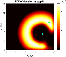
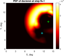
Figure 4: The decision-making process under the policy learned for FPOC corresponding to conditions $e_{t}=0.2$, $e_{n}=0.1$. At the step $n$ observer fixates the location marked by a blue cross. The policy $\mu$ defines a probability density function of a decision $D$ where to fixate next (31). Observer chooses the decision $D_{n}$ according to the policy, which results in a saccadic eye-movement to location $A_{n+1}=\alpha(D_{n})$ (the green cross). As well as in the case of dynamics under the heuristic policy $\pi_{0}$ previously visited locations are inhibited from the subsequent fixations. Note that movements to remote locations are inhibited by the radial function. This results in co-directed short movements, which are also characteristic of human observer.

In supplementary materials A.1 we justify this choice of the policy and evaluate the form of a kernel function $K$ that allows us to effectively solve the optimization problem with the policy gradient algorithms. Our task is the search of the kernel function $K$ (30), which corresponds to the policy that optimizes the cost function $V_{\mu}$:

$$K^{*}=\underset{K}{\arg\min}\>V_{\mu(K)}(S_{0})$$ (20)

for any starting world state $\forall S_{0}$. The policy $\mu(K^{*})$ is called the optimal policy of gaze allocation.

We approach the optimization problem (20) with an algorithm named "REINFORCE with optimal baseline” [32] according to the procedure described in Supplementary materialA. The performance of REINFORCE was compared with one of the optimization algorithms named "policy gradient parameter exploration” (PGPE) adopted from [33]. The algorithm of REINFORCE with an optimal baseline belongs to the class of the likelihood ratio methods, whereas PGPE is related to the finite difference methods. Despite the distinction between these two approaches, both algorithms give a close estimation of the optimal policy A.4.1. We simulated trajectories for the data analysis in section 4 using the solution provided by REINFORCE due its better performance comparing to PGPE. Figure 4 demonstrates the decision-making process under the policy $\mu$ learned for FPOC corresponding to the conditions $e_{t}=0.2$, $e_{n}=0.1$ (see figure 13 for its kernel function). At the step $n$ the observer fixates the location marked by a blue cross. The policy $\mu$ defines a probability density function of the decision $D$ where to fixate next (31). The observer chooses the decision $D_{n}=\mu\left(p_{n}\right)$, which results in a saccadic eye-movement to the location $A_{n+1}=\alpha(D_{n})$ (green cross). As well as in the case of dynamics under the heuristic policy $\pi_{0}$, previously visited locations are inhibited from the subsequent fixations.

4 Basic properties of trajectories

In this section we discuss the statistical properties of trajectories generated with the learned policy $\mu$ and the heuristic policies $\pi_{0}$ and $\pi_{1}$. The simulations were performed on the grid with size $128\times 128$ that corresponds to the visual field with size of $15\times 15\deg$ in the psychophysical experiment. In order to justify our computational model, we reproduced the psychophysical experiments from [9]. The detailed description of the experiments can be found in AppendixC.

4.1 Performance

Although this computational model was not designed for an exact prediction of a response time of human observers, it demonstrates a high level of consistency in a performance of the visual task execution with human observers. The performance was measured as an average time to reach the target (the mean response time) and as a percentage of the correct fixations on target’s location on an N-Alternative Forced Choice task (N-AFC). The unsuccessful trials from the psychophysical experiments were excluded from the consideration. We found that the number of the unsuccessful trials grows with the contrast of noise: $2.3\%$, $5.7\%$, $9.8\%$, $16.4\%$ for the corresponding numbers of the contrast $\epsilon_{n}=$ $(0.1$, $0.15$, $0.2$, $0.25)$.

Figure 5 (left) demonstrates the percentage of correct fixations on the target location for the experimental conditions: $e_{t}=0.2$, $e_{n}=0.15$. Means and standard errors of the response time of the human observers is presented on Figure 5 (right) together with means of the response time for three policies estimated from $10^{4}$ episodes of PO-MDP. The learned policy outperforms two heuristics and the human observers both in the mean response time and the percentage of the correct fixations for all experimental conditions. Human observers significantly outperformed the infomax rate for the experimental conditions: $e_{n}=(0.2,0.25)$ (Student’s t-test $p<0.05$) and the infomax greedy for the conditions $e_{n}=(0.15,0.2,0.25)$ ($p<0.05$) on the mean response time, which was previously found in [22, 9]. In the same time the learned policy outperformed the human observers significantly for the condition $e_{n}=0.25$, while for other conditions t-test didn’t reject hypothesis that distributions have equal means at $5\%$ significance level.

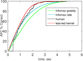
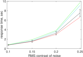
Figure 5: The performance of the human observers and the simulated agents. The learned policy outperforms two heuristics both in the mean completion time and the percentage of correct responses in N-AFC task (left) for the experimental conditions: $e_{t}=0.2$, $e_{n}=0.15$. The dependence of mean completion time (right) for the learned policy resembles one for the human observer.

4.2 Amplitude distribution

The Figure 6 (left) shows the length distributions of saccades of the human observers and the simulated agents performing the visual search task corresponding to the experimental conditions: $e_{n}=0.2$, $e_{t}=0.2$.

The distributions for all policies and the human observers exhibit an ascent between $0\deg$ and maximum around $2\deg$. The difference in the behaviour of the distributions starts from $4\deg$. In this experimental conditions the share of the saccades of the human observer with the length larger than $4\deg$ is $18\%$, whereas this value for $\pi_{0}$ is $38\%$. The length distribution for $\pi_{0}$ stabilizes on the interval $[4.0,14.0]\deg$ that was observed in the earlier work [11], and we found that length of this "stability" interval increases linearly with the grid size. The reason behind this is an uniform radial ranking of policy $\pi_{0}$ for all locations due to the constant radial function (15). The decline of probability starts only at a distance compared to the size of visual field.

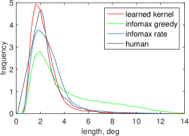
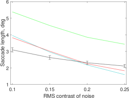
Figure 6: The histograms of the length distribution of the saccadic events (left) for trajectories generated under the policies $\pi_{0},\pi_{1}$ and $\mu_{conv}$ and the human eye-movements corresponding to the experimental conditions: $e_{n}=0.2$, $e_{t}=0.2$. The data was binned with the resolution of $0.1\deg$. The distribution function for all policies and human observer exhibits an ascent between $0\deg$ and maximum around $2$ $\mathrm{deg}$. The distribution of length corresponding tothe infomax greedy $\pi_{0}$ stabilizes after $4$ $\mathrm{deg}$ and declines only after $10$ $\mathrm{deg}$. It is not consistent with length distribution of human saccadic eye-movements, which is concave on an interval $\left[4.0\textdegree,14.0\textdegree\right]$. The mean length of saccades decreases with $e_{n}$ (right). It’s immediate consequence of the decrease of the width of FPOC with $e_{n}$, which defines the area of inhibition from the subsequent fixations.

On the other hand the length distributions of trajectories under $\mu,\pi_{1}$ are concave on an interval $[4.0,14.0]\deg$, which is also a characteristic for human eye-movement [34, 35]. The behaviour of the radial function of $\mu$ reflects the non-uniform radial ranking (a preference in decision-making, see figure (4)) of the locations. As a result, the remote locations have significantly lower probabilities to be chosen as the next destinations.

We performed Kolmogorov-Smirnov (K-S) test to check equality of distributions of experimental and simulated saccades. The results of the test are summarized in table 1 . The first and the second columns show the values of RMS contrast in the psycho-physical experiment and corresponding critical values of the test statistics at a significance level $\alpha=0.01$. The critical values are different due to the difference in number of saccades for each experimental condition. The next three columns show K-S test statistics for the distributions of the saccades simulated under the different policies. K-S test indicated a higher statistical similarity between the distributions of the experimental saccades and the saccades simulated under the learned policy $\mu$ for the cases $e_{n}=(0.15,0.2,0.25)$. In the case $e_{n}=0.1$ the infomax rate and the learned policy explained the experimental distribution equally well. From this, we can make a conclusion that simulations under the learned policy explained the best the length distribution of the human eye-movements.

Cases	K-S test statistics
noise contrast	critical value	infomax greedy	infomax rate	learned policy
0.1	0.067	0.312	0.121	0.124
0.15	0.052	0.256	0.082	0.081
0.2	0.047	0.212	0.053	0.04
0.25	0.035	0.201	0.095	0.074

Table 1: Statistics for K-S test between the experimental distribution of saccade length and simulated distributions for different policies. The first and the second columns show the values of RMS contrast in the psycho-physical experiment and corresponding critical values of test statistics for significance level $\alpha=0.01$. The next three columns show K-S test statistics for distribution of saccades simulated under different policies.

The mean length of the saccades was estimated from $10^{4}$ episodes of PO-MDP for all three policies and compared with the mean length of the saccades of the human observers (see figure 6 right). According to our results, the mean length of the saccades decreases with $e_{n}$, which is consistent with our simulations. It’s an immediate consequence of the decrease of values of FPOC with the increase of the RMS contrast of noise, which is illustrated on figure 2. The amplitude of the signal exceeds the amplitude of noise within the circle area with radius $r$ that satisfies the condition $F(r)=1$ (we call this radius the "width of FPOC”). This circle area is effectively inhibited from the subsequent fixations (see figures (3) and (4)), because information is already gathered with a sufficient level of confidence. However, we found that our model provides close estimates of the mean length only for high values of the RMS contrast of noise. Our experimental findings are consistent with previously reported results [36], where the visual search experiments were set for several levels of the RMS contrast of background noise. In future works we plan to incorporate more complex saccade execution model that takes into account the bias toward the optimal saccade length [17] in order to explain a lower variability of the saccade length in the experiments.

4.3 Geometrical persistence

In this section we analyze the distribution of the directional angle $\theta_{d}$ (this notation was introduced in [10]) of the human saccadic eye-movements and the simulated trajectories. The directional angle is the angle between two consequent saccades, and, therefore, can be defined as $\theta_{d}=\tan^{-1}\left(y_{n+1}/x_{n+1}\right)-\tan^{-1}\left(y_{n}/x_{n}\right)$, where $\left(y_{n},x_{n}\right)$ are the coordinates of $n$th fixation. According to this definition, the movement is related to a persistent one if the directional angle is close to $0$ or $2\pi$. The angles with the values close to $\pi$ correspond to anti-persistent movements.

The distributions of the directional angle were calculated for the trajectories generated by Markov decision process with the policies $\pi_{0},\pi_{1}$ and $\mu$. Figure (7)(left) demonstrates the distribution of the directional angle of the saccadic events for the human observers and the simulated trajectories for $e_{n}=0.2$ and $e_{t}=0.2$. The infomax greedy policy $\pi_{0}$ generates the trajectories with stable anti-persistent movements, because the policy $\pi_{0}$ chooses the next fixation location without taking the current location into consideration. Due to the inhibitory behavior of infomax, it’s much less likely to choose the nearby location instead of remote and relatively unexplored ones. Only geometrical borders limit the choice of the next fixation, which results in fixations on the opposite side of the visual field (as the most remote point, look at the figure (3)).

In contrast, the decision process under the learned policy $\mu$ tends to preserve the direction of the movement. The dynamic of the system under the policy $\mu$ is quite similar to self-avoiding random walk model described in [1]. Due to the asymptotic behavior of the kernel function $K(x,y)$, the reward gain from the remote locations is suppressed, meanwhile, the locations, which are already visited, are also inhibited (look at the figure (4)). This results in short-range self-avoiding movements, which demonstrate the persistent behavior [37, 1], and, therefore, the probability distribution of the directional angle $\theta_{d}$ is biased towards values $0$ or $2\pi$. According to the Figure 7 (left), the dynamics under the heuristics $\pi_{1}$ is also characterized as a persistent random walk. The learned policy $\mu$ has, in general, a stronger radial ranking of locations than $\pi_{1}$, which results in a shorter range of saccades, and a repulsion, caused by inhibition, becomes more relevant. The distribution of average length of saccades depending on $\theta_{d}$ is shown on Figure 7 (right). On average the co-directed movements are shorter than the reversal ones for all policies.

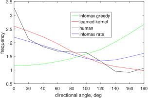
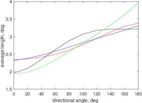
Figure 7: The histograms of the directional angle (left) and the distributions of the mean length of the saccades to the directional angle (right). Data for both histograms was binned with the resolution of 20 $\deg$. The infomax greedy policy $\pi_{0}$ generates the trajectories with stable anti-persistent movements (left), with a high degree of separation between large and small movements (right). In contrast, the decision-making process under the infomax rate policy $\pi_{1}$ tends to preserve the direction of movement. The dynamics under the learned policy $\mu$ is also characterized as a persistent random walk.

In our experiments we discovered that the geometrical persistence depends on the visibility of target (on FPOC in the simulations). We measured the share of the saccades, which retain the direction of the previous movement: $\cos(\theta_{d})>0$. This quantity is called “persistence coefficient”. The figure 8 demonstrates the dependency of the persistence coefficient on the RMS contrast of background noise for the human observers and the simulated trajectories. As it was mentioned previously, the average saccade length is decreasing with the growth of RMS contrast (6). Therefore, the linear term (10) in the duration of steps becomes less relevant, and the decision-making becomes more agnostic about the temporal costs (closer to the information greedy $\pi_{0}$). The decline of the persistent coefficient is also a characteristic of human eye movements, which was not covered in the previous research.

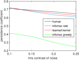
Figure 8: The share of saccades, which retain the direction of the previous movement: $cos(\theta_{d})>0$, is called the "persistence coefficient". This quantity demonstrates the dependence of the persistence on the visibility of the target. As it was mentioned previously, the average saccade length is decreasing with the growth of the RMS contrast (6). Therefore, the linear term (10) in the duration of the steps becomes less relevant, and the decision-making becomes more agnostic about temporal costs (closer to the information greedy $\pi_{0}$). The decline of the persistent coefficient is also a characteristic of the human eye movements, which was not covered in the previous research.

5 Statistical persistence

In the previous section we have analyzed the geometrical persistence of the human eye-movements and the trajectories simulated under three different policies. However, this statistical property doesn’t give any insight into a long-range correlation in time-series. In this section we show that dynamics under the learned policy $\mu$ have a multifractal behavior, which is similar to that of the human eye-movements during execution of the visual search task .

In contrast to the previous research [10] in our analysis we distinguish between two different types of the multifractality by a calculation of a generalized Hurst exponent for shuffled time series. We separate the time series on fixational and saccadic eye-movements, which allows us to demonstrate the fundamental difference in the temporal structure of these types of eye-movements. It was shown that the behaviour of the generalized Hurst exponent is consistent with the basic statistical properties of eye-movements. After this we demonstrate that the dynamics under the optimal policy of gaze allocation explains the changes in scaling behaviour of eye-movements with difficulty of the visual task both on qualitative and quantitative levels.

For statistical analysis of simulated trajectories we use a multifractal detrended fluctuation analysis (MF-DFA)[38], which is a widely-used method for detection of long-range correlations in stochastic time-series. It has found successful applications in the field of bioinformatics [39, 40], nano and geo-physics [41]. This method is based on the approximation of trends in time-series and the subtraction of detected trends (detrending) from original data on different scales. The detrending allows deducting the undesired contribution to long-range correlation, which is a result of non-stationarities of physical processes. We use the package provided by Espen Ihlen [42] for all our estimations of the generalized Hurst exponent in this section.

In the appendix B we thoroughly explain the details of the multifractal analysis. The subsection B.1 presents the details of MF-DFA algorithm. In the subsections B.3 and B.3 we explain how MF-DFA is performed over the simulated trajectories. The results of the multifractal analysis of the human eye-movements are presented in 5.1. The subsection 5.2 summarizes our findings and compares the generalized Hurst exponent of the simulated trajectories to one of human eye-movements for different experimental conditions.

5.1 Multifractality of human eye movements

We perform MF-DFA over the difference of time series of the human gaze positions and in order to compare the estimated generalized Hurst exponent with the simulations. The differentiated time series was estimated from raw data of coordinates of the gaze fixations $A=\left\{\left(x_{1},y_{1}\right),...\left(x_{N},y_{N}\right)\right\}$with the resolution of $7$ ms:

$$\Delta X=\left\{\left(x_{2}-x_{1}\right),\ldots\left(x_{N}-x_{N-1}\right)\right\}$$ (21)

$$\Delta Y=\left\{\left(y_{2}-y_{1}\right),\ldots\left(y_{N}-y_{N-1}\right)\right\}$$ (22)

The time series $\Delta X$ and $\Delta Y$ were estimated for each trial with certain experimental conditions and concatenated over all participants. After this, we represent the differentiated time series in the following way: $\Delta X=\left\{F_{1},S_{1},....,F_{m-1},S_{m-1},F_{m}\right\}$, where $F_{i}$ and $S_{i}$ correspond to the sequences of the movements during time interval of $i$-th fixation and saccade respectively [10]. We separate the differentiated time series on the fixational and the saccadic time series:

$$\Delta X_{F}=\left\{F_{1},0_{s_{1}},\ldots F_{m-1},0_{s_{m}},F_{m}\right\}$$ (23)

$$\Delta X_{S}=\left\{0_{f_{1}},S_{1},\ldots 0_{f_{m-1}},S_{m},0_{f_{m}}\right\}$$ (24)

where $0_{n}$ corresponds to zero array with the length $n$, and $f_{m}$ and $s_{m}$ are the lengths of corresponding sequences $F_{m}$ and $S_{m}$.

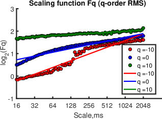
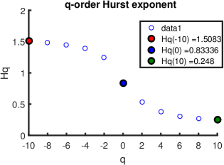
Figure 9: The scaling of the q-order fluctuation function $F_{q}(s)$ (left), and the generalized Hurst exponent $H(q)$ (right) computed through a linear regression of $\log_{2}\left(F_{q}(s)\right)$. This graph is a result of application of MF-DFA over the horizontal differentiated time series $\Delta X$ of the concatenated human scan-paths for the experimental conditions: $e_{t}=0.2$, $e_{n}=0.25$. The red, blue and green lines correspond to the linear approximation of function $\log_{2}\left(F_{q}(s)\right)$ for the orders $q=\left\{-10;0;10\right\}$. The scaling of $F_{q}(s)$ exhibits the crossover the crossover on a time scale of $256$ $ms$. The crossover separates the "lower" and the "upper" regimes mentioned in [10]. The lower regime is related to fixational eye-movements (which is supported by the value of crossover scale s_cros being close to average fixation duration), and the upper regime - to saccadic ones. The crossover in the scaling of $F_{q}(s)$ was observed for all experimental conditions.

The figure 9 demonstrates the scaling of the q-order fluctuation function $F_{q}(s)$ (39). This graph is a result of the application of MF-DFA over the horizontal concatenated differentiated time series $\Delta X$ of the human scan-paths for the experimental conditions: $e_{t}=0.2$, $e_{n}=0.25$. The red, blue and green lines correspond to the linear approximation of function $\log_{2}\left(F_{q}(s)\right)$ for the orders $q=\left\{-10;0;10\right\}$. The scaling of $F_{q}(s)$ exhibits the crossover on a time scale of $256$ $ms$. The crossover separates the "lower” and "upper” regimes mentioned in [10]. According to Amor et. al. the crossover is caused by the presence of two different generative mechanisms of eye-movements. The lower regime is related to fixational eye-movements (which is supported by the value of crossover scale s_cros being close to the average fixation duration), and upper regime - to the saccadic ones. The crossover in the scaling of $F_{q}(s)$ was observed for all experimental conditions. The value of generalized Hurst exponent $H(q)$ (Figure 9 right) is obtained through linear regression of $\log_{2}\left(F_{q}(s)\right)$. Our estimates of $H(q)$ are consistent with the ones of Amor et. al. for both directions and all regimes.

In order to distinguish between two different types of multifractality [38] we calculated the generalized Hurst exponent $H_{shuf}(q)$ for the shuffled differentiated time series. The first type of multifractality is a consequence of a broad probability density function for the values of time series. If only multifractality of the first type presents in time series: $H(q)=H_{shuf}(q)$. The second type of multifractality is caused by the difference in correlation between large and small fluctuations, which is a scenario described in [10]. In this case $H_{shuf}(q)=0.5$ and $H(q)=0.5+H_{corr}(q)$, where $H_{corr}(q)$ is (negative) positive for the long-range (anti-)correlation. If both types of multifractality present in time series: $H(q)=H_{shuf}(q)+H_{corr}(q)$.

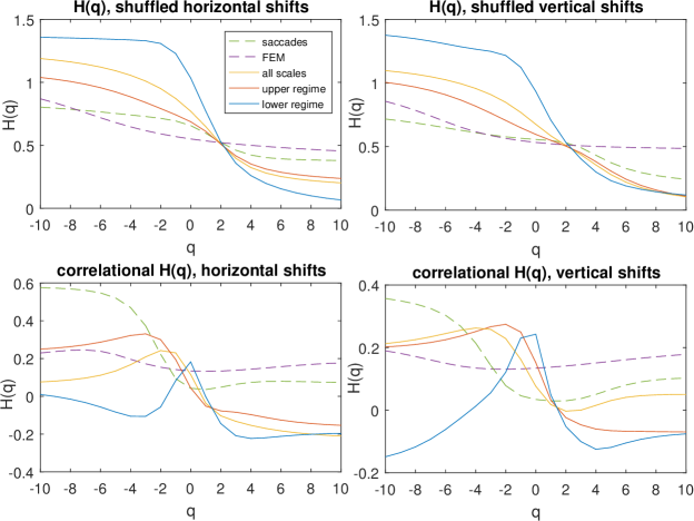
Figure 10: The Hurst exponent of the shuffled time series $H_{shuf}(q)$ (top) and the correlational Hurst exponent $H_{corr}(q)$ (bottom) for the horizontal (left) and the vertical components (right) of the human eye-movements. As well as a previous graph 9, this one is a result of an application of MF-DFA over the concatenated human scan-paths for the experimental conditions: $e_{t}=0.2$, $e_{n}=0.25$. The behaviour of $H_{shuf}(q)$ for both horizontal and vertical shifts for full scales corresponds to the one mentioned in [38] (eq. 27). We assume that multifractality of the first type is caused by an asymptotic behaviour of the amplitude distribution of saccades (see figure 6). The difference in the long-range correlation of large and small fluctuations is reflected by $H_{corr}(q)$ (figure 10 bottom). Due to the properties of the fluctuation function 39 for positive (negative) $q$-orders the main contribution are coming from segments containing small (large) fluctuations [38]. The positive (negative) long range correlation ($H_{corr}(q)>0$) is, therefore, a characteristic of small (large) fluctuations in the upper and the full scales regimes for both directions. In general, these results are consistent with the distribution of the average length of saccades to the directional angle (see figure 7 right), which also indicates the difference in persistence of large and small saccades.

The figure 10 demonstrates our estimates of the Hurst exponent of the shuffled time series $H_{shuf}(q)$ (top) and the correlational Hurst exponent $H_{corr}(q)$ (bottom) for the horizontal (left) and the vertical components (right). We estimated both exponents for the saccades (green dashed line) and FEM (purple dashed line) in the upper and the lower regimes of scales respectively. As well as a previous graph 9, this one is a result of an application of MF-DFA over the concatenated differentiated time series of the human eye-movements for the experimental conditions: $e_{t}=0.2$, $e_{n}=0.25$. The behaviour of $H_{shuf}(q)$ for the full time series and the saccadic time series in the upper regime corresponds to the one mentioned in [38] (eq. 27):

$$H(q)\sim\begin{cases}\begin{array}[]{c}1/q\,\,\,\,\left(q>\alpha\right)\\ 1/\alpha\,\,\,\,\left(q\leq\alpha\right)\end{array}\end{cases}$$ (25)

with $\alpha\sim 1$. The equation 25 was derived for time series of uncorrelated random values with the power law distribution:

$$P=\left\{\begin{array}[]{c}\alpha x^{-(\alpha+1)}\,\,\,\,x\geq 1\\ 0\,\,\,\,\,x<1\end{array}\right.$$ (26)

One can see a similarity of the function (26) with the distribution of the amplitude of the saccadic events for humans (see figure 6). The amplitude distribution of the saccades demonstrates the power law behavior on the interval $\left[4.0\textdegree,14.0\textdegree\right]$ with $\alpha\approx 1$. The probability distribution function (26) also reflects an absence of saccades with the length lower than minimal one. Therefore, the first type of multifractality of the saccadic time series is caused by the broad probability distribution of saccade magnitude.

The difference in the long-range correlation of large and small fluctuations is reflected by $H_{corr}(q)$ (figure 10 bottom). Due to the properties of fluctuation function (39) for the positive (negative) $q$-orders the main contribution are coming from segments containing the large (small) fluctuations [38]. The positive (negative) long-range correlation ($H_{corr}(q)>0$) is, therefore, a characteristic of the small (large) fluctuations in the upper regime for the saccadic and the full time series. These results are consistent with the distribution of the average length of saccade to the directional angle (see figure 7 right), which also indicates the difference in the persistence of large and small saccades. Therefore, we confirm here that the small saccadic eye-movements demonstrate the long-range correlations as well as fixational eye-movements.

The time series of FEM demonstrates the monofractal behaviour and the positive correlations with $H\approx 0.8$ in the lower regime of scales [10]. However, the behaviour of both $H_{corr}(q)$ and $H_{shuf}(q)$ for the full time series in the lower regime indicates the presence of multifractalities of both types. At the present moment we have no explanation of the multifractality in the lower regime and leave this problem for a future work.

5.2 Dependence on visibility

In this section we present a comparison of the generalized Hurst exponent for the human eye-movements in the upper regime and the simulated trajectories under the learned policy. As well as in the case of the geometrical persistence, we claim the quantitative properties of the statistical persistence depend on the visibility of the target.

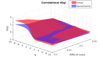
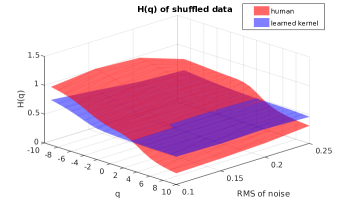
Figure 11: This figure demonstrates $H_{corr}(q)$ (left) of the simulated trajectories (blue) under the learned policy $\mu$ and the correlational Hurst exponent for the human eye-movements (pink) averaged over two directions: $H_{corr}(q)=\left(H_{corr}^{x}(q)+H_{corr}^{y}(q)\right)/2$ in the upper regime. The correlational Hurst exponents for negative $q$-orders declines with the growth of RMS contrast of noise both for human eye-movements and the simulated trajectories. For the positive $q$-orders the correlational Hurst exponent is less affected by the change of the visibility of the target. In general, the correlations weaken with the growth of the RMS contrast, which is consistent with the decline of the geometrical persistence 8. The Hurst exponent of the shuffled time series (right), as well as the correlational Hurst exponent, demonstrates the decline with the growth of the RMS contrast for negative q-orders both for the human eye-movements and the simulated trajectories. In the subsection (5.1) we mentioned that the behaviour of $H_{shuf}(q)$ resembles the one related to time series of random values with power law distribution 26.

We estimated the correlational Hurst exponent $H_{corr}(q)$ and the Hurst exponent of the shuffled time series $H_{shuf}(q)$ for the differentiated trajectories of the human eye-movements for all levels of the RMS contrast of background noise: $e_{n}\in\left(0.1,0.15,0.2,0.25\right)$. Figure 11 (left) shows $H_{corr}(q)$ (left) of simulated trajectories (blue) under the learned policy $\mu$ and the correlational Hurst exponent for the human eye-movements (pink) averaged over two directions: $H_{corr}(q)=\left(H_{corr}^{x}(q)+H_{corr}^{y}(q)\right)/2$ in the upper regime. The correlational Hurst exponents for the negative $q$-orders declines with the growth of the RMS contrast of background noise both for the human eye-movements and the simulated trajectories. This indicates the weakening of the correlation between small fluctuations. For the positive $q$-orders the correlational Hurst exponent is less affected by the change of the visibility of target. The $H_{corr}(q)$ for $q=10$ stabilized on values $0.04$ and $-0.12$ for human eye-movements and the simulated trajectories correspondingly. In general, the correlations weaken with the growth of the RMS contrast, which is consistent with the decline of the geometrical persistence 8. The decline of the Hurst exponent with the increase of difficulty of visual search task was also observed in the previous work [12].

The Hurst exponent of the shuffled time series (Figure 11 right), as well as the correlational Hurst exponent, demonstrates the decline with the growth of the RMS contrast for the negative q-orders both for the human eye-movements and the simulated trajectories. In the subsection 5.1 we mentioned that the behaviour of $H_{shuf}(q)$ resembles the one related to time series of random values with the power law distribution 26. The average value of this time series equals $1/\left(\alpha-1\right)$ for $\alpha>1$. The increase of $\alpha$ results both in the decrease of the average value in time series and the decrease of the value of $H_{shuf}(q)\sim 1/\alpha$ for $q<0$. Therefore, the average value in time series and the values of $H_{shuf}(q)$ for the negative $q$-orders are correlated in the assumption of the power-law distribution. Previously we found the decrease of the average saccade length with the growth of RMS of background noise 6, which is consistent with the decrease of values of $H_{shuf}(q)$ for negative $q$-orders. We assume that this correlation is caused by the power-law asymptotic behaviour of the length distribution of human eye-movements (26).

6 Conclusion

We have presented a computational model of the ideal observer that both qualitatively and quantitatively describes the human visual behaviour during the execution of the visual search task. The basis of this model is the observer’s representation of the constraints of its own visual and oculomotor systems. We demonstrated that a consideration of the temporal costs and uncertainty of the execution of saccades results in the dramatic change of the basic statistical properties and the scaling behavior of the simulated time series.

We performed the multifractal analysis of our data and discovered the presence of two types of multifractality both in time series of the human eye-movements and the model simulations. The multifractality caused by the broad amplitude distribution of the saccades (the first type of multifractality) makes a significant contribution to the multifractal behaviour of time series, which was not covered in the previous work [10]. After the estimation of the correlational part of the Hurst exponent [38] we confirmed the presence of the long-range positive correlations of the small saccades in the upper regime. On the contrary, the large saccades exhibit the weak long-range anti-correlations for the model simulations and the human eye-movements in the upper regime. As well as in the case of the geometrical persistence, we found that the long-range correlations between eye-movements weaken with the decline of the target’s visibility, which is consistent with the previous work on this topic [12].

In this research we focused our attention more on the persistence of eye-movements rather than on their spatial distribution. That’s why we didn’t consider the factors that are not directly related to the trade-off between the temporal costs and the expected information gain. We estimate the optimal policy under the assumption that the visual search process is characterized by shift-rotational symmetry [20], which was not observed in the previous work with similar experimental settings [22]. The symmetry of the visual search can be broken by angular dependency of FPOC in both cases of normal controls and patients with vision disabilities [43]. We plan to include the angular dependency to radial and smoothing functions of policy (see eq. (30)) in order to consider the asymmetry of the visual field in our future works.

To sum up, this framework provides an elegant explanation of scaling and persistent dynamic of the voluntary saccades from an optimality point of view. It clearly demonstrates that control models are able to describe human eye-movements far beyond their basic statistical properties.

Appendix A Implementation of reinforcement learning algorithms

A.1 Kernel function

We assume that the process of the visual search is characterized by shift-rotational invariance [13]. In this research we focus our attention on the persistence of eye-movements rather than on their spatial distribution. That’s why we use the approximation of the shift-rotational invariance in which we don’t need to consider the factors that are not directly related to the trade off between the temporal costs and the expected information gain, such as an asymmetry of FPOC.

The coefficients in the set of dynamic equations (4,6,11) are unaltered under any distance preserving transformations. The last dynamic equation, which is the policy of gaze allocation (18), should be shift-rotational invariant as well. The policy (18) is determined by function of an expected reward $f(D,p)$. Due to the property of shift invariance we can represent the function of an expected reward with Volterra series [44]:

$$f(D,p)=f_{0}+\sum_{n=1}^{N}\sum_{l_{1}=1}^{L}\cdots\sum_{l_{n}=1}^{L}K_{n}(D-l_{1},..,D-l_{n})\prod_{j=1}^{n}p(l_{j})$$ (27)

Where $K_{n}(l_{1},..,l_{n})$ are called Volterra kernels. The constant $f_{0}$ is eliminated in the equation 18, and, therefore, will not be considered. The dimensionality of Volterra kernels $K_{n}$ scales with the number of the potential locations as $L^{n}$. The estimation of Volterra kernel for $n\geq 2$ is computationally unfeasible for the grid size in our simulations: $L=2^{7}\times 2^{7}$. For this reason we consider only the linear term:

$$f(D,p)=\sum_{l}K(D-l)p(l)$$ (28)

We do not expect that the estimation of higher order terms will result in improvement of the performance of the policy. The current observation model 4 is based on independent inputs $W_{l}$ on each individual location, which results in independence of the values of the probability distribution $p_{l}$ for a sufficiently large grid size. Therefore, higher order terms don’t provide additional information on the location of the target.

The function of the expected reward should be computed taking into account the current location of the gaze $A$. Considering its rotational invariance the most general form of this function is: $f(D,p)=\underset{l}{\sum}K(\left\|D-l\right\|,\left\|D-A\right\|)p(l)$. The softmax policy (18) for the function of the expected reward is:

$$\mu(D_{n},p_{n})\propto$$

$$\exp\left(\underset{l}{\sum}p_{n}(l)K\left(\left\|D_{n}-l\right\|,\left\|D_{n}-A_{n}\right\|\right)\right)$$ (29)

Together with the set of the equations (4,6,11), this form of the policy keeps the evolution of the system invariant under any distance-preserving transformation. The convolution of the probability distribution with the kernel function $K(x,y)$ in general form 29 is difficult to optimize, and the problem can be effectively solved only in a separable approximation:

$$K(\left\|D_{n}-A_{n}\right\|,\left\|D_{n}-x\right\|)$$

$$\approx R\left(\left\|D_{n}-A_{n}\right\|\right)S\left(\left\|D_{n}-x\right\|\right)$$ (30)

We call $R$ and $S$ the radial and the smoothing functions correspondingly. The first one characterizes the dependence of the expected reward on the intended saccade length. The motivation behind the introduction of the radial function $R$ are both growing uncertainty of the fixation placement (6) and the duration of the step (11) with the length of the saccade. We assume that the radial function $R$ equals zero outside an interval $\left[a_{min},a_{max}\right]$, where $a_{min}$ and $a_{max}$ are minimal and maximal saccade length correspondingly. The minimal saccade length $a_{min}=1\deg$ [45] is chosen as a magnitude of the shortest possible voluntary movement. The maximal saccade length $a_{max}=\sqrt{2}\cdot 15\deg$ is equal to the length of the diagonal of the stimulus image in our experiments. The smoothing function $S$ describes the relative contribution of the surrounding locations to the reward. The smoothing function has the same role as a term $F$ (see eq. (15)) in the definition of the information maximization policy $\pi_{0}$, and it basically defines how meaningful the certain location is without consideration of the time costs of a relocation.

The form of policy (29) in the separable approximation is:

$$\mu(D_{n},p_{n})\propto$$

$$\exp\left(R\left(\left\|D_{n}-A_{n}\right\|\right)\left(p_{n}*S\right)\left(D_{n}\right)\right)$$ (31)

which is used in the simulation of the trajectories and the training phase. Two heuristic policies presented in section 3.1 are both special cases of the general form of a policy in the separable approximation(31).

A.2 Parametrization of policy

The radial $R(x)$ and the smoothing $S(x)$ functions are represented with Fourier-Bessel series:

$$R(x)=\begin{cases}\begin{array}[]{c}\sum_{\xi=1}^{\varXi}r_{\xi}J_{1}\left(\frac{u_{1:\xi}(x-a_{min})}{a_{max}-a_{min}}\right),\;a_{min}<x<a_{max}\\ 0,\;\;\;\;\;\;\;\;\;else\end{array}\end{cases}$$ (32)

$$S(x)=\begin{cases}\begin{array}[]{c}\sum_{\xi=1}^{\varXi}s_{\xi}J_{0}\left(\frac{u_{0:\xi}x}{b}\right),\;x<b\\ 0,\;\;\;\;\;\;\;\;else\end{array}\end{cases}$$ (33)

where $u_{i:\xi}$ are zeros of Bessel function of order i and $b$ is the radii of the visual field. This representation allows us to control the dimensionality of the kernel and to effectively store the policy in memory. The choice of orders ($i=0,1$) of Bessel functions in (32,33) is caused by boundary conditions for the radial and the smoothing functions: $R(a_{min})=R(a_{max})=0$; $S(b)=0$. The boundary conditions on the radial function forbid the model observer to fixate the same location again $R(0)=0$ and to make unlikely large saccades $R(a_{max})=0$. The condition on the smoothing function $S(b)=0$ corresponds to the absence of any information gain from remote locations, and, therefore, their irrelevance to the process of fixation selection. So, the policy $\mu(\vartheta)$ is represented by set of parameters: $\vartheta\equiv\left(r_{0:\Xi},s_{0:\varXi}\right)$.

A.3 REINFORCE

We solve the optimization problem for the value function (12) with a policy gradient algorithm adopted from [32]. This optimization procedure is represented as an iterative process of a gradient estimation and an update of the policy parameters at the end of each training epoch - the sequence of $M$ episodes.

Repeat

1. Perform a training epoch with $M$ episodes and get the sequence of observations, actions and costs for each time step $t$ and episode $m$: $\left(p_{t,m},a_{t,m},V_{m}\right)$.

2. Estimate optimal baseline for each gradient element $\xi$: $b_{\xi}=\frac{\underset{m}{\sum}\left(\underset{t}{\sum}\nabla_{\xi}\log\mu_{\vartheta}\left(a_{t,m},p_{t,m}\right)\right)^{2}V_{m}}{\underset{m}{\sum}\left(\underset{t}{\sum}\nabla_{\xi}\log\mu_{\vartheta}\left(a_{t,m},p_{t,m}\right)\right)^{2}}$

3. Estimate the gradient for each element: $\eta_{\xi}=\underset{m}{\sum}\left(\underset{t}{\sum}\nabla_{\xi}\log\mu_{\vartheta}\left(a_{t,m},p_{t,m}\right)\right)^{2}\left(b_{\xi}-V_{m}\right)$

4. Update policy parameters: $\vartheta\leftarrow\vartheta+\alpha\eta$

until

gradient $\eta$ converges.

A.4 PGPE

The second approach to the optimization problem (12) is a parameter exploring policy gradient presented in [33]. As well as in the previous section, we estimate the gradient and update the policy parameter at the end of each training epoch. We use a symmetric sampling of the policy parameters for gradient estimation. At the beginning of each step we generate the perturbation $\epsilon$ from normal distribution $N(\mathbf{0},\boldsymbol{I}\mathbf{\boldsymbol{\sigma}}^{2})$ and create the symmetric parameter samples $\vartheta^{+}=\mu+\epsilon$ and $\vartheta^{+}=\mu-\epsilon$, where $\mu$ is the current values of the policy parameters for the training epoch. Then we simulate one episode for each parameter sample and denote the cost $V^{+}$ for the episode generated with $\vartheta^{+}$ , and $V^{-}$ for $\vartheta^{-}$ correspondingly. At the end of each training epoch the policy parameters and the standard deviation of the distribution of perturbation are updated according to the equations:

$$\mu_{i}=\mu_{i}+\alpha\sum_{j=1}^{M}\epsilon_{j}^{i}\left(V_{j}^{-}-V_{j}^{+}\right)$$ (34)

$$\sigma_{i}=\sigma_{i}+\alpha\sum_{j=1}^{M}\left(\frac{\left(\epsilon_{j}^{i}\right)^{2}-\sigma_{i}^{2}}{\sigma_{i}}\right)\left(\left\langle V\right\rangle-\frac{V_{j}^{+}+V_{j}^{-}}{2}\right)$$ (35)

where for $j$th episode $\epsilon_{j}^{i}$ is the perturbation for the parameter $i$ and $V_{j}^{\pm}$ are sampled costs. The cost baseline is chosen as a mean cost for the training epoch.

A.4.1 Convergence of policy gradient

The Markov decision process defined by set of dynamic equations (4,6,11,31) was simulated on $N\times N$ grid, which comprises the $N^{2}$ possible target locations, where $N$=128. At the beginning of the optimization procedure we pick the policy parameters $\vartheta$ randomly from the uniform distribution $U(-0.5,0.5)$ and fix parameter $\lambda=0.001$. For both algorithms we use the same parametrization of policy. The training epoch for both PGPE and REINFORCE consists of 400 episodes. Learning rate $\alpha=0.2$ was the same for both algorithms.

Figure 12 illustrates the performance of two policy gradient methods we used for search of the optimal policy for the case of FPOC corresponding to $e_{n}=0.25$ and $e_{t}=0.2$. Both algorithms used Fourier-Bessel parametrization of policy with a dimensionality $\varXi=45$ for the radial and the smoothing functions. REINFORCE performed better for all parameter settings. On average, it takes around 50 and 40 learning epochs to converge for REINFORCE and PGPE correspondingly. The choice of the dimensionality higher than 45 doesn’t improve the performance of both algorithms.

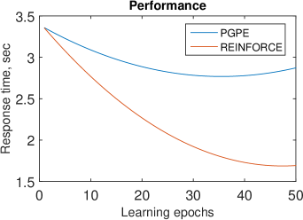
Figure 12: The performance of parameter exploration policy gradient (PGPE) and episodic REINFORCE with an optimal baseline.

Figure 13 shows the results of optimization: the radial $R(x)$ and the smoothing $S(x)$ functions. Both REINFORCE and PGPE provide close estimates of the smoothing and the radial functions for eccentricity smaller than $\epsilon<3\textdegree$. In order to compare the solution with the heuristic policies (15,17), we presented FPOC on the same plot with the smoothing function. The smoothing function provided by REINFORCE is monotonously decreasing as well as FPOC, whereas for PGPE we have a fluctuating solution with a decreasing amplitude of oscillations. The behavior of the radial function is similar for both solutions, with higher amplitude of oscillations for PGPE solution.

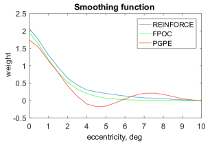
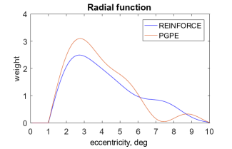
Figure 13: The results of the optimization: the smoothing S(x) funtion (left) and the radial R(x) function (right).

Appendix B Implementation of MF-DFA

B.1 Multifractal analysis

In this chapter we present the details of MF-DFA algorithm used here for calculation of the generalized Hurst exponent. All of this section is based on Kantelhardt et al.[38].

The procedure of MF-DFA starts with definition of a profile for time series $X=\left\{x_{1},...,x_{N}\right\}$ with a compact support:

$$Y(i)=\sum_{k=1}^{i}\left(x_{k}-\left\langle x\right\rangle\right)$$ (36)

The profile $Y(i)$ is divided on $N_{s}\equiv\mathrm{int}(N/s)$ segments, where $s$ is chosen among some linear space $s\in S=\left\{s_{min,}s_{min}+\triangle s,...,s_{max}\right\}$. The segmentation starts from the beginning of time series, therefore, there are residual $N\div s$ number of the elements at the end of time-series. In order to process the residual elements, the segmentation is also performed from the end of time series. So, at the end of segmentation procedure we have $2N_{s}$ segments for each value of $s$.

The calculation of the variance is based on an approximation of local trend for each segment $\nu=1,...,N_{s}$ with a polynomial function $y_{v}$. Then, the variance on each segment is calculated as:

$$F^{2}(\nu,s)=\frac{1}{s}\sum_{i=1}^{s}\left\{Y\left[\left(\nu-1\right)s+i\right]-y_{v}(i)\right\}$$ (37)

for each segment $\nu=1,...,N_{s}$ and

$$F^{2}(\nu,s)=\frac{1}{s}\sum_{i=1}^{s}\left\{Y\left[N-\left(\nu-N_{s}\right)s+i\right]-y_{v}(i)\right\}^{2}$$ (38)

for $\nu=N_{s}+1,...,2N_{s}$. The order m of polynomial function must satisfy the condition $m\leq s-2$. The variance over all segments are averaged to obtain the $q$th order fluctuation function:

$$F_{q}(s)=\left\{\frac{1}{2N_{s}}\sum_{\nu=1}^{2N_{s}}\left[F^{2}(\nu,s)\right]^{q/2}\right\}^{1/q}$$ (39)

According to the properties of $q$th order fluctuation function [46], the scaling behavior of $F_{q}(s)$ is governed by the generalized Hurst exponent:

$$F_{q}(s)\sim s^{H(q)}$$ (40)

The value of $H(q)$ is usually obtained through a linear regression of $\log_{2}\left(F_{q}(s)\right)$.

B.2 Interpolation of simulated trajectories

We perform MF-DFA analysis on the magnitude of the saccadic events simulated by MDP defined above. Each episode of MDP provides the sequence of vectors of gaze positions: $\mathbf{A}_{1},...,\mathbf{A}_{N}$. In order to get the time series of the gaze allocation in real time - $\bar{A}$, we follow the simple procedure of an interpolation:

• The calculation of the duration of each time step $n$ with 11, the total time of episode $T=\sum_{i=1}^{N}\Theta_{i}$ and start time of each discrete step:

  $$T_{n}=\left\{\begin{array}[]{c}0,\,if\,n=1\\ \sum_{i=1}^{n-1}\Theta_{i},\,if\,n>1\end{array}\right.$$ (41)

• The choice of the length of the real-time sequence $M=25*T$, which corresponds to 40 millisecond resolution.

• For each element $t$ of $\mathbf{\bar{A}}$ we define, which discrete time step it belongs: $T_{n}\leq\frac{t}{25}<T_{n+1}$.

• If time step $t$ of $\mathbf{\bar{A}}_{t}$ corresponds to the fixation during the discrete time step $n:$ $\frac{t}{25}-T_{n}<\varTheta_{fix}(n)$, than $\mathbf{\bar{A}}_{t}=\mathbf{A}_{n}$. In the other case, if time $t$ corresponds to the saccadic movement within the discrete time interval n, we have: $\mathbf{\bar{A}}_{t}=\mathbf{A}_{n}+\tau_{sac}\frac{\mathbf{A}_{n+1}-\mathbf{A}_{n}}{\left|\mathbf{\mathbf{A}_{n+1}-\mathbf{A}_{n}}\right|}\left(\frac{t}{25}-T_{n}-\varTheta_{fix}(n)\right)$. Therefore, we have defined the function that maps the discrete sequence $A$ to real-time sequence $\bar{A}$.

The real-time sequences $\bar{A}$ from 1000 episode corresponding to each policy are merged, and the resulting sequences $\bar{A}_{\mu},\bar{A}_{\pi 1},\bar{A}_{\pi 0}$ are analyzed with MF-DFA.

B.3 Multifractality of simulated trajectories

We perform MF-DFA over the differentiated trajectories generated with PO-MDP under the heuristic policies $\pi_{0},\pi_{1}$ and the learned policy $\mu$. Before differentiation trajectories were represented as real time sequences with the procedure of the interpolation B.2.

The model presented here is not devoted to FEM and can’t describe the combined movement of both FEM and the saccades. The results of our analysis should be compared with the scaling behavior of $F_{q}(s)$ for human eye-movements on the scales $s\geq 256$ $ms$, which corresponds to the upper regime. Therefore, we set the minimal time scale $s_{min}=256ms$. The choice of $s_{max}=2*10^{3}ms$ corresponds to the average length of episode. We assume that there is no correlation between the episodes due to a random location of the first fixation and the location of the target.

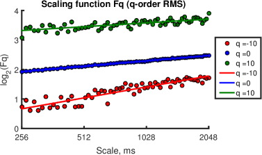
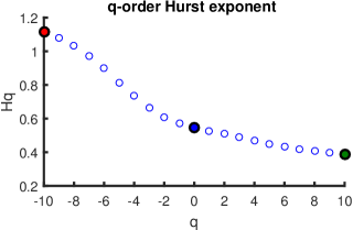
Figure 14: The scaling of the q-order fluctuation function $F_{q}(s)$ (left) estimated for the simulated trajectories under the infomax rate policy $\pi_{1}$, and the generalized Hurst exponent $H(q)$ (right) computed through a linear regression of $\log_{2}\left(F_{q}(s)\right)$. The red, blue and green lines correspond to the linear approximation of function $\log_{2}\left(F_{q}(s)\right)$ for orders $q=\left\{-10;0;10\right\}$. The scaling of $F_{q}(s)$ doesn’t exhibit the crossover for the positive q-orders on an interval of scales $\left[s_{min,}s_{max}\right]$.

The figure 14 demonstrates the scaling of the q-order fluctuation function $F_{q}(s)$ (39) for simulated trajectory under the infomax greedy policy $\pi_{0}$ for the conditions: $e_{t}=0.2$, $e_{n}=0.15$. The red, blue and green lines correspond to the linear approximation of the function $\log_{2}\left(F_{q}(s)\right)$ for the orders $q=\left\{-10;0;10\right\}$. The scaling of $F_{q}(s)$ doesn’t exhibit the crossover for positive q-orders on an interval of scales $\left[s_{min,}s_{max}\right]$, however the behavior of $\log_{2}\left(F_{q}(s)\right)$ deviates from linear at the large scales $s\sim s_{max}$. The simulations on different grid sizes, which correspond to different average time of task execution, have shown that the interval of linear behavior of $\log_{2}\left(F_{q}(s)\right)$ always coincides with $\left[s_{min,}s_{max}\right]$. The scaling of $F_{q}(s)$ on $\left[s_{min,}s_{max}\right]$ is different for different orders $q$ and, therefore, the trajectories $\bar{A}_{\pi_{1}}$ are multifractal time series.

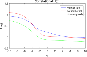
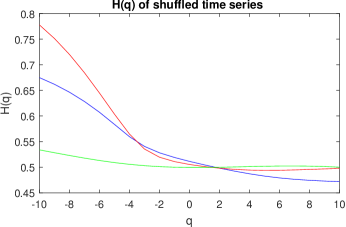
Figure 15: The Hurst exponent of the shuffled time series $H_{shuf}(q)$ (right) and the correlational Hurst exponent $H_{corr}(q)$ (left) of the trajectories simulated under the different policies. As well as in the case of human eye-movements, two types of multifractality present in the simulated time series. The behavior of $H_{shuf}(q)$ resembles the power-law distribution scenario 25 for all policies, except the infomax greedy $\pi_{0}$. The distribution of saccade length doesn’t correspond to the power-law for $\pi_{0}$ , which was demonstrated on the figure 6 . On the contrary, the infomax rate $\pi_{1}$ and the learned policy $\mu$ generate the movement with the distributional multifractality that presents in human eye-movements as well.

The figure 15 demonstrates our estimates of the correlational Hurst exponent $H_{corr}(q)$ (left) and the Hurst exponent of shuffled time series $H_{shuf}(q)$ of time series simulated under the different policies. As well as in the case of the human eye-movements, two types of multifractality present in the simulated time series. The behavior of $H_{shuf}(q)$ resembles the power-law distribution scenario 25 for all policies, except the infomax greedy $\pi_{0}$. The distribution of the saccade length doesn’t correspond to the power-law for $\pi_{0}$ , which was demonstrated on figure 6 . On the contrary, the infomax rate $\pi_{1}$ and the learned policy $\mu$ generate the movement with the distributional multifractality that presents in human eye-movements as well.

For all policies the correlational Hurst exponent is positive for the negative $q$-orders. This indicates the presence of long-range correlations for small fluctuations. The large fluctuations are anticorrelated for $\pi_{1}$ and exhibit weak anti-correlation for $\mu$. We observe the last scenario for upper regime of human eye-movements 10, where the large fluctuations demonstrate a weak anticorrelation in a contrary to positively correlated small fluctuations.

Appendix C Implementation of psychophysical experiments

We set a goal to reproduce the eye tracking experiment described in [11]. In this section we provide the description of the psychophysical experiments.

C.1 Participants

The group of nine patients with normal to corrected-to-normal vision participated in the experiment. The group included four postgraduate students (age $23\pm 7$, 4 males) from Queen Mary University of London. This group was aware of the experimental settings and passed 10 minutes of training sessions with four different experimental conditions, which correspond to the certain value of the RMS contrast of background noise. The experiments were approved by the ethics committee of Queen Mary University of London and informed consent was obtained.

C.2 Equipment

We used DELL P2210 22” LCD monitor (resolution $1680\times 1050$, refresh rate 60 Hz) driven by a Dell Precision laptop for all experiments. The eye movements of the right eye were registered using Eye Tracker device SMI-500 with a sampling frequency of $120$ Hz. The Eye tracker device was mounted on the monitor. Matlab Psychtoolbox was used to run the experiments and generate the stimulus images.

C.3 Stimulus and procedure

The participants set in front of the monitor with their heads fixed with a chin rest at a distance of 110 $cm$ from the monitor. The monitor subtended a visual angle of $21\times 15\deg$. Each participant was shown the examples of the stimulus image before the experiments and was instructed to fixate the target object as fast as possible and to press the certain button on a keyboard to indicate that they found the target. All four participants completed one practice session with 40 trials before the experiment.

The stimuli were the static images generated before each session according to the description from the original experiment [11]. The 1/f noise was generated on a square region on the screen, which spans the visual angle of $15\times 15\deg$. The target was sine grating $6\deg^{-1}$ framed by symmetric raised cosine. The target appeared randomly at any possible location on the stimuli image within the square region. The experiments were provided for one level of RMS contrast of target $e_{t}=0.2$ and several levels of 1/f noise RMS contrast $e_{n}\in(0.1,0.15,0.2,0.25)$.

The participants completed four experimental sessions with 120 trials. The experimental session started after inbuilt nine-point grid calibration of the eye-tracking device. The participants were given 3 minutes of rest between sessions. One of 120 stimuli images were shown at the beginning of each trial. The participants are assumed to perform the visual search task, which is finished by pressing the "END" button. In our experimental settings, the signal from the participants was blocked for $300$ $ms$ from the start of each trial. If the gaze position measured by the eye tracking device is in the vicinity of $2$ $\deg$ around the location of the target at the moment participant presses the "END" button, the task is considered successful. Due to the presence of a temporal delay between the moments of localization of target and pushing of "END" button we block the signal from END button for $400$ $ms$. After a completion of each trial the central fixation cross was shown for $500$ $ms$, then the next trial started and new stimulus image was shown to participants.

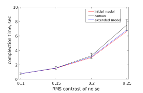
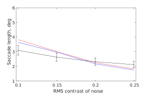
Figure 16: The completion time (left) and the saccade length (right) for the human observers, the simulated agents with the initial observation model and the extended one.

Appendix D Influence of saccade latency

According to the literature, the saccade programming is assumed to be the two-stage process that consists of labile and non-labile stages [17]. The labile stage is the first stage of the saccade programming, during which the initial saccade command can be cancelled in a favour of saccade to another location. The saccade to the next location is executed after the non-labile stage. The visual input is active during both labile and non-labile stages and suppressed during the execution of a saccade. Therefore, the decision $D_{n}$ is made at the end of the labile stage, and the visual input received at the location $A_{n}$ during non-labile stage of saccade programming can be used for decision-making only at the next step $n+1$. As a result, the observer receives two separate observation vectors $\mathbf{W^{n+1}_{lb}}$ and $\mathbf{W^{n+1}_{nlb}}$ from the previous and the current fixation locations. The observation model 4 doesn’t take into account the duration of the observation. We assume that observation vector is integrated continuous-time Gaussian white noise: $W(l,A)=\int_{t}^{t+\varTheta}w(t,l,A)dt$, which satisfies following:

1. $E[w(t,l,A)]=\delta_{l,m}/\theta_{0}$

2. $E[w(t_{1},l_{1},A),w(t_{2},l_{2},A)]=\frac{\delta_{t_{1},t_{2}}\delta_{l_{1},l_{2}}}{\theta_{0}F^{2}\left(\left\|l-A\right\|\right)}$

where $\theta_{0}=250$ $ms$ is a time interval is the detection experiment [11], for which the visibility maps were measured. This model of noise generalizes the "noisy observation" paradigm for variable fixation duration. The result of integration of continuous time noise $w$ is Gaussian white noise $W$ with mean $\varTheta\cdot E[w]$ and variance $\varTheta\cdot\sigma^{2}[w]$. Next, we assume that the duration of the non-labile stage is $\varTheta_{nlb}=41,6$ $ms$ [47] and the rest of fixation duration is allocated for the labile stage $\varTheta_{lb}\approx 200$ $ms$ (the average fixation duration according to our data: $\varTheta_{fix}=240$ ms). Using 1 and 2 we compute mean and variance of observation inputs $\mathbf{W^{n+1}_{lb}}$ and $\mathbf{W^{n+1}_{nlb}}$ , and successively apply the equation 3 to evaluate the belief state $p_{n+1}$.

We learned the policy of gaze allocation for the extended observation model using REINFORCE. We compared the basic characteristic of trajectories simulated under this policy with the simulations for the initial model and data from the human observers (Look at 16. The initial model outperformed the extended one, but no significant difference was found. We didn’t expect any significant difference in performance, because the observer receives the same amount of information on average in both models.

References

References

- Engbert et al. [2011] R. Engbert, K. Mergenthaler, P. Sinn, A. Pikovsky, An integrated model of fixational eye movements and microsaccades, Proceedings of the National Academy of Sciences 108 (39) (2011) E765–E770.
- Engbert and Mergenthaler [2006] R. Engbert, K. Mergenthaler, Microsaccades are triggered by low retinal image slip, Proceedings of the National Academy of Sciences 103 (18) (2006) 7192–7197.
- Engbert and Kliegl [2004] R. Engbert, R. Kliegl, Microsaccades keep the eyes’ balance during fixation, Psychological Science 15 (6) (2004) 431–431.
- Tatler et al. [2011] B. W. Tatler, M. M. Hayhoe, M. F. Land, D. H. Ballard, Eye guidance in natural vision: Reinterpreting salience, Journal of vision 11 (5) (2011) 5.
- Borji and Itti [2013] A. Borji, L. Itti, State-of-the-art in visual attention modeling, Pattern Analysis and Machine Intelligence, IEEE Transactions on 35 (1) (2013) 185–207.
- Ballard and Hayhoe [2009] D. H. Ballard, M. M. Hayhoe, Modelling the role of task in the control of gaze, Visual cognition 17 (6-7) (2009) 1185–1204.
- Ko et al. [2010] H.-k. Ko, M. Poletti, M. Rucci, Microsaccades precisely relocate gaze in a high visual acuity task, Nature neuroscience 13 (12) (2010) 1549–1553.
- Sinn and Engbert [2015] P. Sinn, R. Engbert, Small saccades versus microsaccades: Experimental distinction and model-based unification, Vision research .
- Najemnik and Geisler [2009] J. Najemnik, W. S. Geisler, Simple summation rule for optimal fixation selection in visual search, Vision Research 49 (10) (2009) 1286–1294.
- Amor et al. [2016] T. A. Amor, S. D. Reis, D. Campos, H. J. Herrmann, J. S. Andrade Jr, Persistence in eye movement during visual search, Scientific reports 6.
- Najemnik and Geisler [2005] J. Najemnik, W. S. Geisler, Optimal eye movement strategies in visual search, Nature 434 (7031) (2005) 387–391.
- Stephen and Anastas [2011] D. G. Stephen, J. Anastas, Fractal fluctuations in gaze speed visual search, Attention, Perception, & Psychophysics 73 (3) (2011) 666–677.
- Butko and Movellan [2010] N. J. Butko, J. R. Movellan, Infomax control of eye movements, IEEE Transactions on Autonomous Mental Development 2 (2) (2010) 91–107.
- Wallot et al. [2015] S. Wallot, C. A. Coey, M. J. Richardson, Cue predictability changes scaling in eye-movement fluctuations, Attention, Perception, & Psychophysics 77 (7) (2015) 2169–2180.
- Grigolini et al. [2009] P. Grigolini, G. Aquino, M. Bologna, M. Luković, B. J. West, A theory of 1/f noise in human cognition, Physica A: Statistical Mechanics and its Applications 388 (19) (2009) 4192–4204.
- van Beers [2007] R. J. van Beers, The sources of variability in saccadic eye movements, The Journal of Neuroscience 27 (33) (2007) 8757–8770.
- Engbert et al. [2005] R. Engbert, A. Nuthmann, E. M. Richter, R. Kliegl, SWIFT: a dynamical model of saccade generation during reading., Psychological review 112 (4) (2005) 777.
- Tian et al. [2013] J. Tian, H. S. Ying, D. S. Zee, Revisiting corrective saccades: role of visual feedback, Vision research 89 (2013) 54–64.
- Lee et al. [2002] S. P. Lee, J. B. Badler, N. I. Badler, Eyes alive, in: ACM Transactions on Graphics (TOG), vol. 21, ACM, 637–644, 2002.
- Butko and Movellan [2008] N. J. Butko, J. R. Movellan, I-POMDP: An infomax model of eye movement, in: 2008 7th IEEE International Conference on Development and Learning, IEEE, 139–144, 2008.
- Bradley et al. [2014] C. Bradley, J. Abrams, W. S. Geisler, Retina-V1 model of detectability across the visual field, Journal of vision 14 (12) (2014) 22–22.
- Najemnik and Geisler [2008] J. Najemnik, W. S. Geisler, Eye movement statistics in humans are consistent with an optimal search strategy, Journal of Vision 8 (3) (2008) 4–4.
- Bartz [1962] A. E. Bartz, Eyemovement latency, duration, and response time as a function of angular displacement., Journal of Experimental Psychology 64 (3) (1962) 318.
- Salthouse and Ellis [1980] T. A. Salthouse, C. L. Ellis, Determinants of eye-fixation duration, The American journal of psychology (1980) 207–234.
- Lebedev et al. [1996] S. Lebedev, P. Van Gelder, W. H. Tsui, Square-root relations between main saccadic parameters., Investigative Ophthalmology & Visual Science 37 (13) (1996) 2750–2758.
- Hooge and Erkelens [1996] I. T. C. Hooge, C. J. Erkelens, Control of fixation duration in a simple search task, Perception & Psychophysics 58 (7) (1996) 969–976.
- Kliegl et al. [2006] R. Kliegl, A. Nuthmann, R. Engbert, Tracking the mind during reading: the influence of past, present, and future words on fixation durations., Journal of experimental psychology: General 135 (1) (2006) 12.
- Rayner et al. [1978] K. Rayner, G. W. McConkie, S. Ehrlich, Eye movements and integrating information across fixations., Journal of Experimental Psychology: Human Perception and Performance 4 (4) (1978) 529.
- Greene [2006] H. H. Greene, The control of fixation duration in visual search, Perception 35 (3) (2006) 303–315.
- Unema et al. [2005] P. J. Unema, S. Pannasch, M. Joos, B. M. Velichkovsky, Time course of information processing during scene perception: The relationship between saccade amplitude and fixation duration, Visual cognition 12 (3) (2005) 473–494.
- Navalpakkam et al. [2010] V. Navalpakkam, C. Koch, A. Rangel, P. Perona, Optimal reward harvesting in complex perceptual environments, Proceedings of the National Academy of Sciences 107 (11) (2010) 5232–5237.
- Peters and Schaal [2006] J. Peters, S. Schaal, Policy gradient methods for robotics, in: 2006 IEEE/RSJ International Conference on Intelligent Robots and Systems, IEEE, 2219–2225, 2006.
- Sehnke et al. [2010] F. Sehnke, C. Osendorfer, T. Rückstieß, A. Graves, J. Peters, J. Schmidhuber, Parameter-exploring policy gradients, Neural Networks 23 (4) (2010) 551–559.
- Tatler et al. [2006] B. W. Tatler, R. J. Baddeley, B. T. Vincent, The long and the short of it: Spatial statistics at fixation vary with saccade amplitude and task, Vision research 46 (12) (2006) 1857–1862.
- Castelhano et al. [2009] M. S. Castelhano, M. L. Mack, J. M. Henderson, Viewing task influences eye movement control during active scene perception, Journal of Vision 9 (3) (2009) 6–6.
- Geisler et al. [2006] W. S. Geisler, J. S. Perry, J. Najemnik, Visual search: The role of peripheral information measured using gaze-contingent displays, Journal of Vision 6 (9) (2006) 1–1.
- Isogami and Matsushita [1992] S. Isogami, M. Matsushita, Structural and statistical properties of self-avoiding fractional Brownian motion, Journal of the Physical Society of Japan 61 (5) (1992) 1445–1448.
- Kantelhardt et al. [2002] J. W. Kantelhardt, S. A. Zschiegner, E. Koscielny-Bunde, S. Havlin, A. Bunde, H. E. Stanley, Multifractal detrended fluctuation analysis of nonstationary time series, Physica A: Statistical Mechanics and its Applications 316 (1) (2002) 87–114.
- Rosas et al. [2002] A. Rosas, E. Nogueira Jr, J. F. Fontanari, Multifractal analysis of DNA walks and trails, Physical Review E 66 (6) (2002) 061906.
- Dutta et al. [2013] S. Dutta, D. Ghosh, S. Chatterjee, Multifractal detrended fluctuation analysis of human gait diseases, Frontiers in physiology 4 (2013) 274.
- Vandewalle et al. [1999] N. Vandewalle, M. Ausloos, M. Houssa, P. Mertens, M. Heyns, Non-Gaussian behavior and anticorrelations in ultrathin gate oxides after soft breakdown, Applied physics letters 74 (1999) 1579.
- Ihlen [2012] E. A. F. E. Ihlen, Introduction to multifractal detrended fluctuation analysis in Matlab, Frontiers in physiology 3 (2012) 141.
- Van der Stigchel et al. [2013] S. Van der Stigchel, R. A. Bethlehem, B. P. Klein, T. T. Berendschot, T. Nijboer, S. O. Dumoulin, Macular degeneration affects eye movement behavior during visual search, Frontiers in psychology 4 (2013) 579.
- Volterra and Long [1944] V. Volterra, M. Long, Theory of Functionals and of Integral and Integro-differential Equations, Blackie and Son Limited, URL https://books.google.co.uk/books?id=iKUVswEACAAJ, 1944.
- Otero-Millan et al. [2008] J. Otero-Millan, X. G. Troncoso, S. L. Macknik, I. Serrano-Pedraza, S. Martinez-Conde, Saccades and microsaccades during visual fixation, exploration, and search: foundations for a common saccadic generator, Journal of Vision 8 (14) (2008) 21–21.
- Peitgen et al. [2006] H.-O. Peitgen, H. Jürgens, D. Saupe, Chaos and fractals: new frontiers of science, Springer Science & Business Media, 2006.
- Engbert et al. [2002] R. Engbert, A. Longtin, R. Kliegl, A dynamical model of saccade generation in reading based on spatially distributed lexical processing, Vision research 42 (5) (2002) 621–636.