Cubature on Wiener Space for McKean-Vlasov SDEs with Smooth Scalar Interaction

Abstract

We present two cubature on Wiener space algorithms for the numerical solution of McKean-Vlasov SDEs with smooth scalar interaction. First, we consider a method introduced in [12] under a uniformly elliptic assumption and extend the analysis to a uniform strong Hörmander assumption. Then, we introduce a new method based on Lagrange polynomial interpolation.

1 Introduction

In this paper, we analyse the error in two different algorithms using Cubature on Wiener space to weakly approximate the solution of a McKean-Vlasov SDE with smooth scalar interaction. By scalar interaction, we mean that the dependence on the measure is through the integral against a scalar function, so the McKean-Vlasov SDE takes the form

$$X_{t}^{x}=x+\int_{0}^{t}V_{0}(X_{s}^{x},\mathbb{E}\varphi_{0}(X_{s}^{x}))\,ds+\sum_{i=1}^{d}\int_{0}^{t}V_{i}(X_{s}^{x},\mathbb{E}\varphi_{i}(X_{s}^{x}))\circ dB^{i}_{s},$$ (1.1)

where $\displaystyle\varphi_{i}\in\mathcal{C}_{b}^{\infty}(\mathbb{R}^{N};\mathbb{R})$, $\displaystyle V_{i}\in\mathcal{C}_{b}^{\infty}(\mathbb{R}^{N+1};\mathbb{R}^{N})$ and $\displaystyle B=\left(B^{1},\ldots,B^{d}\right)$ is a Brownian motion. We wish to approximate $\displaystyle\mathbb{E}\left[f(X_{T}^{x})\right]$ for $\displaystyle f$ Lipschitz continuous and $\displaystyle T>0$ a fixed time.

One common way of approaching this problem is to consider a discretisation of the equation, such as the Euler-Maruyama scheme, along with a Monte Carlo approximation. At each time step, an approximation of the law of $\displaystyle X_{t}^{x}$ is then given by the empirical distribution of the entire Monte Carlo population. However, estimating the error due to approximating the expectation inside the coefficients by the Monte Carlo estimator is exactly the problem one wishes to solve in the first place. This leads to a more difficult analysis than for classical SDEs. Nonetheless, this analysis has been carried out under a number of different assumptions when the coefficients have the form $\displaystyle V_{i}(X_{t}^{x},\textstyle\int h_{i}(X_{t}^{x}-y)\,P_{X_{t}^{x}}(dy)),$ (slightly different to (1.1)). This type of scheme was studied in papers by Bossy, alone [3] and along with Talay [4]; Kohatsu-Higa & Ogawa [16], and Antonelli & Kohatsu-Higa [1]. In all of these papers the total error is composed of a discretisation error of order $\displaystyle\sqrt{h}$ or $\displaystyle h$, where $\displaystyle h$ is size of the largest time step, and statistical error of order $\displaystyle N_{MC}^{-1/2}$ where $\displaystyle N_{MC}$ is the number of Monte Carlo samples. A Milstein discretisation is also analysed in Ogawa [26]. In [28] Tachet des Combes proposes a deterministic numerical scheme based on discretising the PDE satisfied by the density function of the solution to (1.1). More recently, in [27], a Multi-Level Monte Carlo scheme has been analysed for equations of the type (1.1).

Cubature on Wiener space is a high-order alternative to Monte Carlo methods. It is part of a class of methods called Kusuoka-Lyons-Victoir methods that have been shown to be highly effective in practice, see e.g. [13], [25]. Applications include the non-linear filtering problem [6, 23, 11, 22], backward stochastic differential equations [8, 9] and calculating Greeks [29] in finance. Convergence of the cubature approximation for some path dependent functionals has also been shown in [2]. The starting point of the Cubature on Wiener space method is to view $\displaystyle X^{x}_{T}$ as a functional of the Brownian path $\displaystyle(B_{s})_{s\in[0,T]}$, say

$$X^{x}_{T}=\alpha_{x,T}((B_{s})_{s\in[0,T]}),\>\>\>\>\alpha_{x,T}:\mathcal{C}_{0}([0,T];\mathbb{R}^{d})\to\mathbb{R}^{N},$$

and to view the expectation $\displaystyle\mathbb{E}[f(X_{T}^{x})]$ as an integral over the Wiener space

$$\mathbb{E}[f(X_{T}^{x})]=\int_{\Omega}\left(f\circ\alpha_{x,T}\right)(\omega)\,\mathbb{P}(d\omega),$$ (1.2)

where $\displaystyle\Omega=\mathcal{C}_{0}([0,T];\mathbb{R}^{d})$ and $\displaystyle\mathbb{P}$ is the Wiener measure. The key idea of the cubature on Wiener space method is that one can approximate such integrals by replacing the Wiener measure, $\displaystyle\mathbb{P}$, by a discrete measure supported on finitely many bounded variation paths, called a cubature measure. If the cubature measure is chosen so that iterated Stratonovich integrals of Brownian motion up to some order have the same expectation under the cubature and Wiener measures and the time interval $\displaystyle[0,T]$ is small, then by considering the Stratonovich-Taylor expansion of the solution of the SDE, one can show that the target expectations under the cubature and Wiener measures agree up to some high order error. When the time interval is not small, $\displaystyle[0,T]$ can be partitioned into sub-intervals and the approximation performed over each sub-interval. In the original paper [24], dealing with ordinary SDEs, evaluating the functional $\displaystyle\alpha_{x,T}$ at a bounded variation path $\displaystyle\omega$ amounts to solving an rdinary differential equation (ODE) and evaluating integrals such as (1.2) under a cubature measure amounts to computing weighted sums of solutions of ODEs. The complication for McKean-Vlasov equations like (1.1) is that the functional $\displaystyle\alpha_{x,T}$ depends on the paths $\displaystyle\left\{(\mathbb{E}\varphi_{i}(X^{x}_{s}))_{s\in[0,T]}:i=0,\ldots,d\right\}$ which are unknown. Instead, one must include an approximation of the functional $\displaystyle\alpha_{x,T}$ in the design of the algorithm.

To our knowledge, the first algorithm involving Cubature on Wiener Space in relation to McKean-Vlasov SDE was introduced by Chaudru de Raynal & Garcia-Trillos [12]. Their idea is to partition $\displaystyle[0,T]$ into $\displaystyle\{0=t_{0}<t_{1}<\ldots<t_{n}=T\}$ and over the interval $\displaystyle[t_{j},t_{j+1}]$ to replace $\displaystyle\mathbb{E}\varphi_{i}(X^{x}_{t})$ appearing in the coefficients with the cubature approximation of the Taylor exapnsion of the path $\displaystyle t\mapsto\mathbb{E}\varphi_{i}(X^{x}_{t})$ around $\displaystyle t_{j}$ up to some order, $\displaystyle q$. The global error can, as in the original case, be decomposed as a sum of local errors, and these local errors naturally split into an error due to the approximation of $\displaystyle\mathbb{E}\varphi_{i}(X^{x}_{t})$ in the coefficients, and an error due to replacing the Wiener measure by a cubature measure. The authors consider the case of smooth and bounded uniformly elliptic coefficients and prove that the error is of order $\displaystyle n^{-[(q+1)\wedge(l-1)/2]}$ where $\displaystyle n$ is the number of time steps and $\displaystyle l$ is the degree of the cubature formula. This is the first algorithm we consider. We show how to extend the error analysis to the case when the coefficients satisfy a uniform strong Hörmander condition. One of the reasons the authors of [12] choose to impose a uniformly elliptic condition on the coefficients of equation (1.1) is the lack of available sharp derivative estimates for time-inhomogeneous parabolic PDEs (which are necessary for the error analysis) under any more general conditions. For this reason, a secondary goal of this work is to develop derivative estimates for time-inhomogeneous parabolic PDEs under more general conditions and to analyse the error for the cubature on Wiener space algorithm in this case.

In the second algorithm, which we call the Lagrange interpolation method, over the interval $\displaystyle[t_{j},t_{j+1}]$, one simply replaces $\displaystyle\mathbb{E}\varphi_{i}(X^{x}_{t})$ with the Lagrange polynomial which interpolates the cubature approximation of $\displaystyle\mathbb{E}\varphi_{i}(X_{t}^{x})$ at the previous $\displaystyle r$ points in the time partition.

1.1 Cubature on Wiener Space

First, we detail exactly what we mean by a cubature formula on Wiener space. We need to introduce notation for iterated integrals with respect to components of the $\displaystyle(d+1)$-dimensional process $\displaystyle(B^{0},B^{1},\ldots,B^{d})$ consisting of time and the $\displaystyle d$-dimensional Brownian motion. We use the following notation for multi-indices on $\displaystyle\{0,\ldots,d\}$:

$$\mathcal{A}:=\{\emptyset\}\cup\cup_{k\geq 1}\{0,1,\ldots,d\}^{k}\quad\text{ and }\quad\mathcal{A}_{1}:=\mathcal{A}\setminus\{\emptyset,(0)\}.$$

We endow $\displaystyle\mathcal{A}$ with the concatenation operation

$$\alpha\ast\beta:=(\alpha_{1},\ldots,\alpha_{k},\beta_{1},\ldots,\beta_{l}),\ \ \text{where }\alpha=(\alpha_{1},\ldots,\alpha_{k}),\ \ \ \beta=(\beta_{1},\ldots,\beta_{l})\in\mathcal{A}.$$

and we define $\displaystyle\alpha^{\prime}=(\alpha_{1})$ and $\displaystyle-\alpha:=(\alpha_{2},\ldots,\alpha_{k})$, so that $\displaystyle\alpha=\alpha^{\prime}\ast-\alpha$. We define the following $\displaystyle n$-tuples lengths:

$$\left|\,\alpha\,\right|:=\begin{cases}k,&\text{if }\alpha=(\alpha_{1},\ldots,\alpha_{k}),\\ 0,&\text{if }\alpha=\emptyset.\end{cases}\>\>\>\>\>\left\|\alpha\right\|:=\left|\,\alpha\,\right|+\text{card }\{i:\alpha_{i}=0,i=1,\ldots,d\},$$

and define the set $\displaystyle\mathcal{A}(l):=\{\alpha\in\mathcal{A}:\|\alpha\|\leq l\}$ and define $\displaystyle\mathcal{A}_{1}(l)$ similarly. For $\displaystyle\alpha\in\mathcal{A}$, we denote by $\displaystyle I^{\alpha}_{t,s}(Y)$ the iterated Stratonovich integral of the process $\displaystyle Y$ over the interval $\displaystyle[t,s]$:

$$I^{\alpha}_{t,s}(Y):=\int_{t}^{s}\int_{t}^{s_{n}}\cdots\int_{t}^{s_{2}}Y_{s_{1}}\circ dB^{\alpha_{1}}_{s_{1}}\cdots\circ dB_{s_{n-1}}^{\alpha_{n-1}}\circ dB_{s_{n}}^{\alpha_{n}}.$$

Similarly, for a bounded variation path $\displaystyle\omega=(\omega^{1},\ldots,\omega^{d})\in\mathcal{C}_{bv}([t,s];\mathbb{R}^{d})$ we set $\displaystyle\omega^{0}(s)=s$ and denote the iterated integral of a process $\displaystyle Y$ by $\displaystyle I^{\alpha}_{t,s}[\omega](Y)$:

$$I^{\alpha}_{t,s}[\omega](Y):=\int_{t}^{s}\int_{t}^{s_{n}}\cdots\int_{t}^{s_{2}}Y_{s_{1}}d\omega^{\alpha_{1}}_{s_{1}}\cdots d\omega_{s_{n-1}}^{\alpha_{n-1}}\,d\omega_{s_{n}}^{\alpha_{n}}.$$

With this notation in hand, we can define a cubature formula.

Definition 1.1 (Cubature formula [24]).

A set of $\displaystyle N_{Cub}$ bounded variation paths,
$\displaystyle\omega_{1},\ldots,\omega_{N_{Cub}}\in\mathcal{C}_{bv}([0,1];\mathbb{R}^{d})$, for some $\displaystyle N_{Cub}\in\mathbb{N}$, together with some weights
$\displaystyle\lambda_{1},\ldots,\lambda_{N_{Cub}}\in\mathbb{R}^{+}$ such that $\displaystyle\textstyle\sum_{j=1}^{N_{Cub}}\lambda_{j}=1$ define a cubature formula on Wiener Space of degree $\displaystyle l$ if, for any $\displaystyle\alpha\in\mathcal{A}(l)$,

$$\mathbb{E}[I^{\alpha}_{0,1}(1)]=\sum_{j=1}^{N_{Cub}}\lambda_{j}\,I^{\alpha}_{0,1}[\omega_{j}](1).$$

We note that for a given $\displaystyle l\in\mathbb{N}$, Lyons & Victoir [24] proved that there exists a cubature formula on Wiener Space of degree $\displaystyle l$, with concrete examples given, for certain pairs $\displaystyle(l,d)$, in [24] and [13]. From the scaling properties of the Brownian motion we can deduce, for $\displaystyle 0\leq t<s$,

$$\mathbb{E}[I^{\alpha}_{t,s}(1)]=\sum_{j=1}^{l}\lambda_{j}\,I^{\alpha}_{t,s}[\omega_{j}(t,s)](1),$$

where $\displaystyle\omega_{j}(t,s)$ is the re-scaled path defined by $\displaystyle\textstyle\omega_{j}(t,s)\left(u\right)=\sqrt{s-t}\,\omega_{j}\left(\frac{u}{s-t}\right)$, $\displaystyle u\in\left[t,s\right]$. In other words, the expectation of the iterated Stratonovich integrals $\displaystyle I^{\alpha}_{t,s}(1)$ with $\displaystyle\alpha\in\mathcal{A}(l)$ is the same under the Wiener measure as it is under the cubature measure,

$$\mathbb{Q}_{t,s}:=\sum_{j=1}^{N_{Cub}}\lambda_{j}\,\delta_{\omega_{j}(t,s)}.$$

Once we have a cubature measure $\displaystyle\mathbb{Q}$ and a partition $\displaystyle\Pi_{n}$, we can extend this to a measure $\displaystyle\mathbb{Q}^{\Pi_{n}}$ on $\displaystyle[0,T]$, supported on $\displaystyle(N_{cub})^{n}$ paths along a tree. We use the notation $\displaystyle\mathcal{M}_{k}$ to denote multi-indices over $\displaystyle\{1,\ldots,N_{Cub}\}$ of length exactly $\displaystyle k$. We use this set to index the nodes in the cubature tree after $\displaystyle k$ time-steps or, equivalently, the unique path leading to that node. To create the tree, one first creates the paths by concatenating the re-scaled paths: for $\displaystyle p=(p_{1},\ldots,p_{n})\in\mathcal{M}_{n}$, define the path

$$\omega_{p}(t)=\omega_{p}(t_{i-1})+\omega_{p_{i}}(t_{i-1},t_{i})(t)\quad\text{ when }t\in[t_{i-1},t_{i}).$$

Then, one can attach a new weight to each path by

$$\Lambda_{p}:=\prod_{p_{i}\in p}\lambda_{p_{i}}.$$

Finally, we can define a measure on all paths along the tree by

$$\mathbb{Q}^{\Pi_{n}}:=\sum_{p\in\mathcal{M}_{n}}\Lambda_{p}\,\delta_{\omega_{p}}.$$

1.2 Outline & Main Results

In this section, let us make more precise our contribution. We introduce the following processes

$$\displaystyle X_{t}^{s,x}=x+\sum_{i=0}^{d}\int_{s}^{t}V_{i}(X_{u}^{s,x},\mathbb{E}\varphi_{i}(X_{u}^{s,x}))\circ dB^{i}_{u},$$ (1.3)

and

$$\displaystyle X_{t}^{s,x,y}=x+\sum_{i=0}^{d}\int_{s}^{t}V_{i}(X_{u}^{s,x,y},\mathbb{E}\varphi_{i}(X_{u}^{0,y}))\circ dB^{i}_{u}.$$ (1.4)

The first is just the McKean-Vlasov SDE started from $\displaystyle x$ at time $\displaystyle s$. The second process is also started from $\displaystyle x$ at time $\displaystyle s$ but with the path $\displaystyle u\mapsto\mathbb{E}[\varphi_{i}(X_{u}^{0,y})]$ appearing in the coefficients instead of the McKean-Vlasov term. This process is therefore not a true McKean-Vlasov process but an SDE with coefficients depending on time and a parameter, $\displaystyle y$. We introduce the operators

$$\displaystyle P_{s,t}f(x):=\mathbb{E}\left[f(X_{t}^{s,x})\right]\quad\text{ and }\quad P_{s,t}^{y}f(x):=\mathbb{E}\left[f(X_{t}^{s,x,y})\right].$$

We note that $\displaystyle X_{T}^{0,x}=\left.X_{T}^{0,x,y}\right|_{y=x},$ so the quantity we wish to compute is

$$P_{0,T}f(x)=\left.P^{y}_{0,T}f(x)\right|_{y=x}.$$

Now, let us denote by $\displaystyle E_{t}^{y}(\varphi_{i})$ a generic approximation of $\displaystyle\mathbb{E}[\varphi_{i}(X_{t}^{0,y})]$. Later, we will introduce specific approximations $\displaystyle E_{t}^{T,y}(\varphi_{i})$ and $\displaystyle E_{t}^{L,y}(\varphi_{i})$, corresponding to the Taylor and Lagrange interpolation methods respectively. We then introduce the approximating process

$${}^{E}X_{t}^{s,x,y}=x+\sum_{i=0}^{d}\int_{s}^{t}V_{i}(^{E}X_{u}^{s,x,y},E_{u}^{y}(\varphi_{i}))\circ dB^{i}_{u},$$

and the operators

$$\displaystyle P_{s,t}^{E,y}g(x):=\mathbb{E}\left[g(^{E}X_{t}^{s,x,y})\right]\quad\text{ and }\quad Q_{s,t}^{E,y}g(x):=\mathbb{E}_{\mathbb{Q}_{s,t}}\left[g(^{E}X_{t}^{s,x,y})\right].$$

In a similar way, we will denote the local approximation operator by $\displaystyle Q_{s,t}^{E,x}$ and, once a partition $\displaystyle\Pi_{n}$ of $\displaystyle[0,T]$ is fixed, we define

$$Q^{E,x,\Pi_{n}}_{0,t}:=Q_{0,t_{1}}^{E,x}\cdots Q^{E,x}_{t_{j},t}\quad\text{ for }t\in[t_{j},t_{j+1}).$$

Then, $\displaystyle Q^{E,x,\Pi_{n}}_{0,T}f(x)$ will be the final approximation of $\displaystyle P_{0,T}f(x)$, with the global error

$$\mathcal{E}(T,x,l,\Pi_{n}):=\left(P_{0,T}-Q^{E,x,\Pi_{n}}_{0,T}\right)f(x).$$

We note that

$$\sup_{x\in\mathbb{R}^{N}}\left|\mathcal{E}(T,x,l,\Pi_{n})\right|\leq\sup_{x,y\in\mathbb{R}^{N}}\left|\left(P^{y}_{0,T}-Q^{E,y,\Pi_{n}}_{0,T}\right)f(x)\right|.$$

Now, for fixed $\displaystyle y$, $\displaystyle\{P^{y}_{s,t}:0\leq s\leq t\leq T\}$ forms a two-parameter semigroup of operators. This allows us to decompose the global error the scheme as follows

$$\displaystyle\left[P^{y}_{0,T}-Q^{E,y}_{0,t_{1}}Q^{E,y}_{t_{1},t_{2}}\cdots Q^{E,y}_{t_{n-1},t_{n}}\right]f(x) \displaystyle=\sum_{j=0}^{N-1}Q^{E,y}_{0,t_{j}}\left[P^{y}_{t_{j},t_{j+1}}-Q_{{t_{j},t_{j+1}}}^{E,y}\right]P^{y}_{t_{j+1},T}f(x).$$

Then, since $\displaystyle\left\|Q^{E,y}_{0,t_{j}}\phi\right\|_{\infty}\leq\|\phi\|_{\infty}$, we are left to estimate the local error

$$\left[P^{y}_{t_{j},t_{j+1}}-Q_{{t_{j},t_{j+1}}}^{E,y}\right]u^{y}(t_{j+1},x)$$

uniformly in $\displaystyle x$ and $\displaystyle y$, where $\displaystyle u^{y}(t,x):=P^{y}_{t,T}f(x)$ solves a parabolic PDE with coefficients depending on the parameter $\displaystyle y\in\mathbb{R}^{N}$. The resulting error analysis relies on regularity estimates for the solution of this PDE.

Now, let us specify what the approximation $\displaystyle E^{x}_{t}(\varphi_{i})$ is for each scheme. First, the Taylor method: we wish to perform a Taylor expansion of the path $\displaystyle t\mapsto\mathbb{E}\varphi_{i}(X^{0,x}_{t})$, but since the coefficients in the SDE satisfied by $\displaystyle X^{0,x}$ are of the form $\displaystyle V_{i}\left(X^{0,x}_{t},\mathbb{E}\varphi_{i}(X^{0,x}_{t})\right)$, we instead consider the Taylor expansion of this more general form. For a pair of functions $\displaystyle g\in\mathcal{C}^{\infty}_{b}(\mathbb{R}^{N}\times\mathbb{R};\mathbb{R})$ and $\displaystyle\varphi\in\mathcal{C}^{\infty}_{b}(\mathbb{R}^{N};\mathbb{R})$, Itô’s formula yields

$$\displaystyle\begin{split}\mathbb{E}&\left[g\left(X^{0,x}_{t},\mathbb{E}\varphi(X^{0,x}_{t})\right)\right]=g\left(x,\varphi(x)\right)\\ &\quad+\int_{0}^{t}\mathbb{E}\left[\left(\mathcal{L}^{x}_{u}g\right)\left(X^{0,x}_{u},\mathbb{E}\varphi(X^{0,x}_{u})\right)\right]+\mathbb{E}\left[(\partial_{y}g)\left(X^{0,x}_{u},\mathbb{E}\varphi(X^{0,x}_{u})\right)\right]\mathbb{E}\left[\left(\mathcal{L}^{x}_{u}\varphi\right)(X^{0,x}_{u})\right]\,du,\end{split}$$ (1.5)

where $\displaystyle\partial_{y}$ is the derivative in the second argument of $\displaystyle g$ and $\displaystyle\mathcal{L}^{x}_{s}$ is the differential operator

$$\displaystyle\mathcal{L}_{s}^{x}:=V_{0}(\cdot,\mathbb{E}\varphi_{0}(X_{s}^{0,x}))+\frac{1}{2}\sum_{i=1}^{d}V_{i}(\cdot,\mathbb{E}\varphi_{i}(X_{s}^{0,x}))^{2}.$$

Note that each term under the integral in the right hand side of (1.5) is again a product of terms of the form $\displaystyle\mathbb{E}\left[g\left(X^{0,x}_{u},\mathbb{E}\varphi(X^{0,x}_{u})\right)\right]$ for different functions $\displaystyle g$ and $\displaystyle\varphi$. Let us denote by $\displaystyle\mathcal{S}$ the set of all paths $\displaystyle(S_{t})_{t\in[0,T]}$ of the form

$$S_{t}=\mathbb{E}\left[g\left(X^{0,x}_{t},\mathbb{E}\varphi(X^{0,x}_{t})\right)\right]$$

for some $\displaystyle g\in\mathcal{C}^{\infty}_{b}(\mathbb{R}^{N}\times\mathbb{R};\mathbb{R})$, and $\displaystyle\varphi\in\mathcal{C}^{\infty}_{b}(\mathbb{R}^{N};\mathbb{R})$ and denote by $\displaystyle\bar{\mathcal{S}}$ the set of all paths $\displaystyle(\bar{S}_{t})_{t\in[0,T]}$ of the form

$$\bar{S}_{t}=\sum_{i=1}^{n_{1}}\prod_{j=1}^{n_{2}}S^{i,j}_{t}$$

where $\displaystyle n_{1}$ and $\displaystyle n_{2}$ are positive integers and $\displaystyle S^{i,j}\in\mathcal{S}$ for $\displaystyle i=1,\ldots,n_{1}$ and $\displaystyle j=1,\ldots,n_{2}$. For $\displaystyle t\in[0,T]$, we introduce the notation $\displaystyle\mathcal{T}:\mathcal{S}\to\bar{\mathcal{S}}$ for the map

$$\displaystyle\mathbb{E} \displaystyle\,g\left(X^{0,x},\mathbb{E}\varphi(X^{0,x})\right)$$

$$\displaystyle\mapsto\mathbb{E}\left[\left(\mathcal{L}^{x}g\right)\left(X^{0,x},\mathbb{E}\varphi(X^{0,x})\right)\right]+\mathbb{E}\left[(\partial_{y}g)\left(X^{0,x},\mathbb{E}\varphi(X^{0,x})\right)\right]\mathbb{E}\left[\left(\mathcal{L}^{x}\varphi\right)(X^{0,x})\right],$$

so that the expansion of $\displaystyle G_{t}:=\mathbb{E}\left[g\left(X^{0,x}_{t},\mathbb{E}\varphi(X^{0,x}_{t})\right)\right]$ in (1.5) can alternatively be written as

$$G_{t}=G_{0}+\int_{0}^{t}\mathcal{T}_{s}(G)\,ds$$ (1.6)

For the Taylor expansion, we would like to apply $\displaystyle\mathcal{T}$ to the term $\displaystyle\mathcal{T}(G)$. To do so, we extend $\displaystyle\mathcal{T}$ to an operator from $\displaystyle\bar{\mathcal{S}}$ to itself by linearity

$$\mathcal{T}\left(\sum_{i=1}^{n_{1}}S^{i}\right)=\sum_{i=1}^{n_{1}}\mathcal{T}\left(S^{i}\right),$$

and a product rule

$$\mathcal{T}\left(\prod_{j=1}^{n_{2}}S^{j}\right)=\sum_{k=1}^{n_{2}}\prod_{j=1,j\neq k}^{n_{2}}S^{j}\>\mathcal{T}\left(S^{k}\right).$$

Since now we have $\displaystyle\mathcal{T}$ defined as an operator on $\displaystyle\bar{\mathcal{S}}$, we can iterate the expansion in (1.6) to get the Taylor expansion of order $\displaystyle q\geq 1$

$$G_{t}=\sum_{k=0}^{q}\frac{t^{k}}{k!}\,(\mathcal{T}_{0})^{k}(G)+\frac{1}{(q+1)!}\int_{0}^{t}\,(\mathcal{T}_{s})^{q+1}(G)\,ds.$$ (1.7)

Now, for all $\displaystyle s\in[0,T]$, $\displaystyle k\geq 1$ and $\displaystyle G\in\bar{\mathcal{S}}$ we define $\displaystyle\left(\mathcal{T}_{s}^{Q}\right)^{k}(G)$ to be the same expression as $\displaystyle\left(\mathcal{T}_{s}\right)^{k}(G)$ with all expectations under $\displaystyle\mathbb{P}$ replaced by expectations under $\displaystyle\mathbb{Q}^{\Pi_{n}}$. Then, the approximation of $\displaystyle\mathbb{E}\varphi_{i}(X^{0,y}_{s})$ for the Taylor method, which we henceforth denote by $\displaystyle E^{T,y}_{s}(\varphi_{i})$, is

$$\displaystyle E^{T,y}_{s}(\varphi_{i}):=\sum_{k=0}^{q}\frac{1}{k!}\,(\mathcal{T}^{Q}_{t_{j}})^{k}(\mathbb{E}\varphi_{i}(X^{0,y}))\,(s-t_{j})^{k}\quad\text{ for }s\in[t_{j},t_{j+1}).$$

We make some explicit computations of this type in Example … in Section 4.

To define the approximation for the Lagrange interpolation method, we denote by $\displaystyle L\left[\left\{(t_{i},x_{i})\right\}_{i=1}^{k}\right]$ the Lagrange interpolating polynomial of degree at most $\displaystyle k-1$ with $\displaystyle L\left[\left\{(t_{i},x_{i})\right\}_{i=1}^{k}\right](t_{j})=x_{j}$ for all $\displaystyle j=1,\ldots,k$. We define the approximation of order $\displaystyle r$ by

$$E^{y}_{t}(\varphi_{i}):=L\left[\left\{\left(t_{j-k},\mathbb{E}^{\mathbb{Q}^{\Pi_{n}}}\varphi_{i}\left(X^{0,y}_{t_{j-k}}\right)\right)\right\}_{k=0}^{j\wedge(r-1)}\right](t)\quad\quad t\in[t_{j},t_{j+1}]$$

In other words, $\displaystyle E^{y}_{t}(\varphi_{i})$ for $\displaystyle t\in[t_{j},t_{j+1}]$ is the unique polynomial of degree minimal degree which passes through the points $\displaystyle\left(t_{j+1-((j+1)\wedge r)},\mathbb{E}^{\mathbb{Q}^{\Pi_{n}}}\varphi(X^{0,y}_{t_{j+1-((j+1)\wedge r)}})\right),\ldots,\left(t_{j},\mathbb{E}^{\mathbb{Q}^{\Pi_{n}}}\varphi(X^{0,y}_{t_{j}})\right)$. That is, if the time index $\displaystyle j$ is greater than $\displaystyle r-1$, we interpolate through the last $\displaystyle r$ cubature approximations of $\displaystyle\mathbb{E}\varphi(X^{0,y}_{t})$ along the partition. If $\displaystyle j<r-1$, we interpolate through all of the available previous points. We now detail both algorithms.

Algorithm 1 Taylor method

1:Set $\displaystyle(X^{\emptyset},\Lambda_{0})=(x,1)$

2:for $\displaystyle 0\leq j\leq n-1$ do

3:     Let $\displaystyle\mathcal{T}^{Q}$ be as in the main text.

4:     for $\displaystyle p\in\mathcal{M}_{j}$ do

5:         for $\displaystyle 0\leq i\leq d$ do

6:              Set $\displaystyle\displaystyle E^{T}_{i}(t)=\sum_{k=0}^{q}\frac{1}{k!}(t-t_{j})^{k}(\mathcal{T}^{Q}_{t_{j}})^{k}(\mathbb{E}\varphi_{i}(X^{0,x}))$

7:         end for

8:         for $\displaystyle 1\leq l\leq N_{cub}$ do

9:              Define $\displaystyle X_{t_{j+1}}^{p*l}$ as the solution of the ODE:

$$\displaystyle dX^{p*l}_{t}=\sum_{i=0}^{d}V_{i}\left(X_{t}^{p*l},E^{T}_{i}(t)\right)\,d\omega_{l}^{i}(t_{j},t_{j+1})(t),$$

$$\displaystyle X^{p*l}_{t_{j}}=X^{p}_{t_{j}}.$$

10:              Set the associated weight: $\displaystyle\Lambda_{p*l}=\Lambda_{p}\lambda_{l}$

11:         end for

12:         for $\displaystyle 0\leq i\leq d$ do

13:              Store $\displaystyle\sum_{p\in\mathcal{M}_{j+1}}\Lambda_{p}\varphi_{i}(X^{p}_{t_{j+1}})$.

14:         end for

15:     end for

16:end for

17:Final approximation of $\displaystyle\mathbb{E}\left[f(X_{T}^{x})\right]$ is

$$\sum_{p\in\mathcal{M}_{n}}\Lambda_{p}f(X^{p}_{t_{n}})$$

Algorithm 2 Lagrange interpolation method

1:Set $\displaystyle(X^{\emptyset},\Lambda_{0})=(x,1)$

2:for $\displaystyle 0\leq j\leq n-1$ do

3:     for $\displaystyle p\in\mathcal{M}_{j}$ do

4:         for $\displaystyle 0\leq i\leq d$ do

5:              Set $\displaystyle E^{L}_{i}(t):=L\left[\left\{\left(t_{j-k},\sum_{p\in\mathcal{M}_{j-k}}\Lambda_{p}\varphi_{i}(X^{p}_{t_{j-k}})\right)\right\}_{k=0}^{j\wedge(r-1)}\right](t)$

6:         end for

7:         for $\displaystyle 1\leq l\leq N_{cub}$ do

8:              Define $\displaystyle X_{t_{j+1}}^{p*l}$ as the solution of the ODE:

$$\displaystyle dX^{p*l}_{t}=\sum_{i=0}^{d}V_{i}\left(X_{t}^{p*l},E^{L}_{i}(t)\right)\,d\omega_{l}^{i}(t_{j},t_{j+1})(t),$$

$$\displaystyle X^{p*l}_{t_{j}}=X^{p}_{t_{j}}.$$

9:              Set the associated weight: $\displaystyle\Lambda_{p*l}=\Lambda_{p}\lambda_{l}$

10:         end for

11:         for $\displaystyle 0\leq i\leq d$ do

12:              for $\displaystyle 0\leq k\leq((j+1)\wedge r)$ do

13:                  Store $\displaystyle\sum_{p\in\mathcal{M}_{j+1-k}}\Lambda_{p}\varphi_{i}(X^{p}_{t_{j+1-k}})$.

14:              end for

15:         end for

16:     end for

17:end for

18:Final approximation of $\displaystyle\mathbb{E}\left[f(X_{T}^{x})\right]$ is

$$\sum_{p\in\mathcal{M}_{n}}\Lambda_{p}f(X^{p}_{t_{n}})$$

Remark 1.2.

The Taylor method requires finding an expression for $\displaystyle(\mathcal{T}_{t})^{k}(\mathbb{E}\varphi_{i}(X^{0,y}))$ for $\displaystyle k=1,\ldots,q$ and $\displaystyle i=0,\ldots,d$ either by hand or using some symbolic computation. The Lagrange interpolation method does not require this; the interpolating polynomial is defined at each time step as part of the algorithm.

Now, we state the main assumptions. First, we introduce the notation $\displaystyle V_{[\alpha]}$ for iterated Lie brackets of the vector fields. In this setting each $\displaystyle V_{0},\ldots,V_{d}:\mathbb{R}^{N}\times\mathbb{R}\to\mathbb{R}^{N}$ and we think of these as vector fields $\displaystyle V_{i}(\cdot,x^{\prime})$ on $\displaystyle\mathbb{R}^{N}$ parametrised by the second variable, $\displaystyle x^{\prime}\in\mathbb{R}$, with the Lie Bracket between any two given by

$$[V_{i},V_{j}](x,x^{\prime})=\partial_{x}V_{j}(x,x^{\prime})V_{i}(x,x^{\prime})-\partial_{x}V_{i}(x,x^{\prime})V_{j}(x,x^{\prime})$$

where $\displaystyle\partial V_{i}(x,x^{\prime}):=(\partial_{x_{l}}V_{i}^{k}(x,x^{\prime}))_{1\leq k,l\leq N}$ is the Jacobian matrix of $\displaystyle V_{i}$ and similarly for $\displaystyle\partial_{x}V_{j}$. Then, for $\displaystyle\alpha\in\bigcup_{k\geq 1}\{1,\ldots,N\}^{k}$ and $\displaystyle i\in\{1,\ldots,N\}$, we define inductively

$$\displaystyle V_{[i]}:=V_{i},\quad\quad V_{[\alpha*i]}:=[V_{i},V_{[\alpha]}]\quad.$$

Now we are able to state our assumptions.

Assumption 1.3.

• Uniform strong Hörmander condition: there exist $\displaystyle\delta>0$ and $\displaystyle m\in\mathbb{N}$ such that for all $\displaystyle\xi\in\mathbb{R}^{N}$,

  $$\displaystyle\inf_{(x,x^{\prime})\in\mathbb{R}^{N}\times\mathbb{R}}\sum_{\alpha\in\cup_{k=1}^{m}\{1,\ldots,N\}^{k}}\langle V_{[\alpha]}(x,x^{\prime}),\xi\rangle^{2}\geq\delta\,\left|\xi\right|^{2}$$

• Smoothness of coefficients:

  $$\displaystyle\varphi_{i}\in\mathcal{C}^{\infty}_{b}(\mathbb{R}^{N};\mathbb{R}),\quad V_{i}\in\mathcal{C}^{\infty}_{b}(\mathbb{R}^{N}\times\mathbb{R};\mathbb{R}^{N})\quad i=0,\ldots,d$$

• We assume the paths in any cubature formula we use are absolutely continuous.

As is common with cubature on Wiener space methods, when the terminal function $\displaystyle f$ is not smooth, we will use an uneven partition of the time interval $\displaystyle[0,T]$. Here, we introduce the Kusuoka partition and a modified version. We denote by $\displaystyle\Pi^{\gamma}_{n}$ the Kusuoka [18] partition of the interval $\displaystyle[0,T]$ with $\displaystyle(n+1)$ points and parameter $\displaystyle\gamma\geq 1$, defined by

$$\displaystyle t_{j}=T\left(1-\left(1-\frac{j}{n}\right)^{\gamma}\right)\quad\text{ for }j=0,\ldots,n-1,$$

$$\displaystyle t_{n}=T.$$

We denote by $\displaystyle\Pi^{\gamma,r}_{n}$ the modified Kusuoka partition, with $\displaystyle r$ smaller steps at the start whose size is determined by the overall order of the method we require. It is defined as follows: for a fixed integer $\displaystyle r$ and real parameter $\displaystyle\gamma$, we fix the first $\displaystyle(r+1)$ points as $\displaystyle t_{0}=0$, $\displaystyle t_{k+1}-t_{k}=Tn^{-r/(k+1)}$ for $\displaystyle k=0,\ldots,r-1$. Thereafter and we split the rest of the interval $\displaystyle[t_{r},T]$ using the Kusuoka partition, i.e.

$$\displaystyle t_{j}=\left(T-t_{r}\right)\textstyle\left(1-\left(1-\frac{j-r}{n-r}\right)^{\gamma}\right)+t_{r}\quad\quad j\in\{r+1,\ldots,n-1\}$$

$$\displaystyle t_{n}=T$$

Then we have the following result, which is the main result of this work.

Theorem 1.4.

Let $\displaystyle f\in\mathcal{C}^{\infty}_{b}(\mathbb{R}^{N};\mathbb{R})$. Then, assuming (A2), the error for the Taylor method satisfies the following

$$\sup_{x\in\mathbb{R}^{N}}\left|\mathcal{E}(T,x,l,\Pi_{n})\right|\leq C\,\sum_{j=0}^{n-1}(t_{j+1}-t_{j})^{A(q,l)},$$

where $\displaystyle A(q,l):=(q+2)\wedge(l+1)/2$. Under the same assumptions, the error in the Lagrange interpolation method is

$$\sup_{x\in\mathbb{R}^{N}}\left|\mathcal{E}(T,x,l,\Pi_{n})\right|\leq C\,\sum_{j=0}^{n-1}\bigg{\{}\frac{(t_{j+1}-t_{j})}{((j+1)\wedge r)!}\prod_{k=0}^{j\wedge(r-1)}(t_{j+1}-t_{j-k})+(t_{j+1}-t_{j})^{(l+1)/2}\bigg{\}}.$$

Now, suppose $\displaystyle f$ is only Lipschitz continuous. Assuming (A1)-(A3) and that we use the Kusuoka partition $\displaystyle\Pi^{\gamma}_{n}$ with $\displaystyle\gamma>l-1$, we can bound the error in the Taylor method according to the size of $\displaystyle m$

$$\displaystyle m=1:\quad\quad \displaystyle\sup_{x\in\mathbb{R}^{N}}\left|\mathcal{E}(T,x,l,\Pi^{\gamma}_{n})\right|\leq C\,n^{-B(q,l)-1/2},$$ (1.8)

$$\displaystyle m\geq 2:\quad\quad \displaystyle\sup_{x\in\mathbb{R}^{N}}\left|\mathcal{E}(T,x,l,\Pi^{\gamma}_{n})\right|\leq C\,n^{-B(q,l)},$$ (1.9)

where $\displaystyle B(q,l)=(q+\textstyle\frac{1}{2})\wedge\frac{l-2}{2}$. Assuming (A1)-(A3) and that we use the modified Kusuoka partition $\displaystyle\Pi^{\gamma,r}_{n}$ with $\displaystyle\gamma\in(l-1,l)$, we can bound the error in the Lagrange interpolation method according to the size of $\displaystyle m$

$$\displaystyle m=1:\quad\quad \displaystyle\sup_{x\in\mathbb{R}^{N}}\left|\mathcal{E}(T,x,l,\Pi^{\gamma,r}_{n})\right|\leq C\,n^{-D(r,l)-1/2}\,(1-r/n)^{-l/2},$$ (1.10)

$$\displaystyle m\geq 2:\quad\quad \displaystyle\sup_{x\in\mathbb{R}^{N}}\left|\mathcal{E}(T,x,l,\Pi^{\gamma,r}_{n})\right|\leq C\,n^{-D(r,l)}\,(1-r/n)^{-l/2},$$ (1.11)

where $\displaystyle D(r,l)=(r-\textstyle\frac{3}{2})\wedge\textstyle\frac{l-2}{2}$.

Remark 1.5.

1. Let us comment on the term $\displaystyle(1-r/n)^{-l/2}$ appearing in the error for the Lagrange interpolation method. This term comes from the need to take small steps at the start (for an accurate polynomial approximation) and end of the partition (due to blow up of the derivatives of $\displaystyle u^{y}(t,\cdot)$). We need to take $\displaystyle r$ small steps at the start, leaving $\displaystyle n-r$ steps split in the style of the Kusuoka partition. This term reflects the need to balance the size of $\displaystyle r$ and $\displaystyle n$. Since it goes to zero as $\displaystyle n\to\infty$, it can be bounded by a constant for sufficiently large $\displaystyle n$. For example, in the case $\displaystyle m=1$ for a second order method, one must use a cubature formula of degree $\displaystyle l=5$ and choose $\displaystyle r=4$. Then, for $\displaystyle n\geq 10$ $\displaystyle(1-r/n)^{-l/2}=(1-4/n)^{-5/2}<3.6$.

2. The uniformly elliptic case covered by [12] is the case $\displaystyle m=1$. Choosing the parameter $\displaystyle r$ appropriately, we also recover the same rate for the Lagrange interpolation method up to the multiplication of the term $\displaystyle(1-r/n)^{-l/2}$.

3. In the case where $\displaystyle m\geq 2$, we lose $\displaystyle 1/2$ an order of convergence. This is due to the difference in the way we split the error, which we explain in Remark 3.1

2 Preliminary results

First, we have a lemma on existence, uniqueness and moment bounds for the solution of equation (1.4).

Lemma 2.1.

Under assumption (A2), there exist unique strong solutions to equations (1.3) and (1.4). Moreover, for all $\displaystyle s\in[t,T]$, the mapping $\displaystyle x\mapsto X_{s}^{t,x,y}$ is $\displaystyle\mathbb{P}$-a.s. smooth, and for all multi-indices $\displaystyle\eta$ on $\displaystyle\{1,\ldots,N\}$,

$$\sup_{x,y\in\mathbb{R}^{N}}\left\|\partial^{\eta}_{x}X^{t,x,y}_{s}\right\|_{p}<\infty\quad\forall p\geq 1.$$ (2.1)

Proof.

Under assumption (A2), existence and uniqueness of strong solutions to equations (1.3) and (1.4) is easy to prove and can be found in, for example, [14]. Now, we note that we can view $\displaystyle\left(X^{t,x,y}_{s}\right)_{s\in[t,T]}$ as the solution of an SDE with coefficients

$$W^{y}_{i}(s,z):=V_{i}(z,\mathbb{E}\varphi_{i}(X^{0,y}_{s})),$$

depending on time and a parameter. Due to Assumption 1.3 (A2) $\displaystyle(s,z)\mapsto W^{y}_{i}(s,z)$ is smooth, with bounded derivatives of all orders, with all bounds uniform in $\displaystyle y$. The differentiability in $\displaystyle z$ is assumed, and the differentiability in $\displaystyle s$ comes from the smoothness of each $\displaystyle\varphi_{i}$, which allows us to apply Itô’s formula to $\displaystyle\varphi_{i}(X^{0,y}_{s})$, giving

$$\partial_{s}\left[\mathbb{E}\varphi_{i}(X^{0,y}_{s})\right]=\mathbb{E}\left[(\mathcal{L}^{y}_{s}\varphi_{i})(X^{0,y}_{s})\right].$$

Then, Kunita [17, Theorem 4.6.5] guarantees that the moment bound (2.1) holds. ∎

In the next lemma, we collect some results on the regularity of $\displaystyle u^{y}(t,x)$ and the pure cubature part of the error. We use the notation, for $\displaystyle\psi\in\mathcal{C}^{2}_{b}(\mathbb{R}^{N};\mathbb{R})$,

$$\|\psi\|_{2,\infty}:=\sup_{x\in\mathbb{R}^{N}}\left\{|\psi(x)|+|\nabla\psi(x)|+|\nabla^{2}\psi(x)|\right\}.$$

Lemma 2.2.

Let $\displaystyle j\in\{0,\ldots,n-2\}$ and $\displaystyle t\in[0,T)$.

1. If $\displaystyle f\in\mathcal{C}^{\infty}_{b}(\mathbb{R}^{N};\mathbb{R})$, then for both schemes corresponding to $\displaystyle E=E^{T}$ and $\displaystyle E=E^{L}$

   $$\displaystyle\sup_{x,y\in\mathbb{R}^{N}}\left|\left[P^{E,y}_{t_{j},t_{j+1}}-Q^{E,y}_{t_{j},t_{j+1}}\right]u^{y}(t_{j+1},x)\right| \displaystyle\leq C\,(t_{j+1}-t_{j})^{(l+1)/2}.$$ (2.2)

   Moreover, the first two derivatives of $\displaystyle u^{y}$ are bounded:

   $$\sup_{(t,y)\in[0,T]\times\mathbb{R}^{N}}\left\|u^{y}(t,\cdot)\right\|_{2,\infty}\leq C.$$ (2.3)

2. If $\displaystyle f$ is Lipschitz, then

   $$\displaystyle\sup_{x,y\in\mathbb{R}^{N}}\left|\left[P^{y}_{t_{j},t_{j+1}}-Q^{y}_{t_{j},t_{j+1}}\right]u^{y}(t_{j+1},x)\right| \displaystyle\leq C\,\sum_{k=l}^{l+1}(T-t_{j+1})^{-k/2}\,(t_{j+1}-t_{j})^{(k+1)/2}.$$ (2.4)

   In addition, the first derivative of $\displaystyle u^{y}$ is bounded

   $$\sup_{(t,x,y)\in[0,T]\times\mathbb{R}^{N}\times\mathbb{R}^{N}}\left|\nabla u^{y}(t,x)\right|\leq C$$ (2.5)

   and we have the estimate on the first two derivatives:

   $$\sup_{y\in\mathbb{R}^{N}}\left\|u^{y}(t,\cdot)\right\|_{2,\infty}\leq C\,(T-t)^{-m/2}.$$ (2.6)

   Finally, for both schemes corresponding to $\displaystyle E=E^{L}$ and $\displaystyle E=E^{T}$,

   $$\sup_{x,y\in\mathbb{R}^{N}}\left|\left[P^{y}_{s,t}-Q_{s,t}^{E,y}\right]f(x)\right|\leq C\,\|f\|_{Lip}|t-s|^{1/2}.$$ (2.7)

Proof.

We think of $\displaystyle\left(X^{t,x,y}_{s}\right)_{s\in[t,T]}$ and $\displaystyle\left({}^{E}X^{t,x,y}_{s}\right)_{s\in[t,T]}$ as the solutions of the SDEs with coefficients

$$\displaystyle W^{y}_{i}(s,z) \displaystyle:=V_{i}(z,\mathbb{E}\varphi_{i}(X^{0,y}_{s})),$$

$${}^{E}W^{y}_{i}(s,z) \displaystyle:=V_{i}(z,E^{y}_{s}(\varphi_{i}))\quad i=0,\ldots,d,$$

respectively. We think of $\displaystyle\left\{W^{y}_{i}(t,\cdot),\>^{E}W^{y}_{i}(t,\cdot):i=0,\ldots,d\right\}$ as vector fields on $\displaystyle\mathbb{R}^{N}$ depending on time $\displaystyle t\in[0,T]$ and the parameter $\displaystyle y\in\mathbb{R}^{N}$. In the proof of Lemma 2.1, we explained that $\displaystyle W^{y}_{0},\ldots,W^{y}_{d}\in\mathcal{C}^{\infty}_{b}([0,T]\times\mathbb{R}^{N};\mathbb{R}^{N})$ with all bounds uniform in $\displaystyle y$. The same is true of the functions ${}^{E}W^{y}_{0}\ldots,^{E}W^{y}_{d}$. To see this, we note that for the both schemes, the map $\displaystyle s\mapsto E^{y}_{s}(\varphi_{i})$ is a polynomial, therefore smooth with bounded derivatives on $\displaystyle[0,T]$.

We use the notation $\displaystyle W^{y}_{[\alpha]}$ and ${}^{E}W^{y}_{[\alpha]}$ for iterated Lie brackets of the vector fields introduced just before Assumption 1.3. Then, we note that for all $\displaystyle(s,z,y)\in[0,T]\times\mathbb{R}^{N}\times\mathbb{R}^{N}$ and $\displaystyle\alpha\in\cup_{k\geq 1}\{1,\ldots,N\}^{k}$,

$$\displaystyle\langle W^{y}_{[\alpha]}(s,z),\xi\rangle^{2}\geq\inf_{x^{\prime}\in\mathbb{R}}\langle V_{[\alpha]}(z,x^{\prime}),\xi\rangle^{2},$$

so that

$$\displaystyle\inf_{(s,z,y)\in[0,T]\times\mathbb{R}^{N}\times\mathbb{R}^{N}}\langle W^{y}_{[\alpha]}(s,z),\xi\rangle^{2}\geq\inf_{(z,x^{\prime})\in\mathbb{R}^{N}\times\mathbb{R}}\langle V_{[\alpha]}(z,x^{\prime}),\xi\rangle^{2}.$$

Hence, under the uniform strong Hörmander condition (A1),

$$\displaystyle\inf_{(s,z,y)\in[0,T]\times\mathbb{R}^{N}\times\mathbb{R}^{N}}\sum_{\alpha\in\cup_{k=1}^{m}\{1,\ldots,N\}^{k}}\langle W^{y}_{[\alpha]}(s,z,y),\xi\rangle^{2}\geq\delta\,|\xi|^{2},$$

so the vector fields $\displaystyle\{W^{y}_{i}:i=1,\ldots d\}$ satisfy a uniform strong Hörmander condition. Exactly the same holds true for the vector fields $\displaystyle\{^{E}W^{y}_{i}:i=1,\ldots d\}$. This uniform strong Hörmander condition is stronger than the $\displaystyle\widetilde{UFG}$ condition, hence, we have the results of Section A.3 available to us, subject to slight modification since the coefficients in the current setting also depend on a parameter.

Now, for $\displaystyle f\in\mathcal{C}^{\infty}_{b}(\mathbb{R}^{N};\mathbb{R})$, by differentiating under the expectation and using the moment bounds on $\displaystyle\partial^{\eta}_{x}X^{t,x,y}_{s}$ contained in (2.1) we see that for all multi-indices $\displaystyle\eta$ on $\displaystyle\{1,\ldots,N\}$ with length at least one,

$$\sup_{x,y\in\mathbb{R}^{N}}\left|\partial^{\eta}_{x}u^{y}(t,x)\right|<\infty,$$

so (2.3) holds. The one step cubature error conrtained in (2.2) follows from a stochastic Taylor expansion, noting that for all $\displaystyle\beta\in\mathcal{A}_{1}$,

$$\sup_{x,y\in\mathbb{R}^{N}}\left|\widetilde{W}^{y}_{\beta}u^{y}(t,x)\right|<\infty.$$

This again follows from the boundedness of derivatives of $\displaystyle u^{y}(t,\cdot)$ and $\displaystyle W^{y}_{i}(t,\cdot)$ uniformly in $\displaystyle y$.

For $\displaystyle f$ Lipschitz, the bound in (2.4) is the same as (A.18), adapted to the case where coefficients also depend on a parameter. The estimate (2.5) comes from Corollary A.9 adapted to the case where coefficients also depend on a parameter.

Finally, when $\displaystyle f$ is Lipschitz,

$$\displaystyle\left|\left[P^{y}_{s,t}-Q_{s,t}^{E,y}\right]f(x)\right| \displaystyle=\left|\mathbb{E}\left[f(X_{t}^{s,x,y})\right]-\mathbb{E}_{\mathbb{Q}}\left[f(^{E}X_{t}^{s,x,y})\right]\right|$$

$$\displaystyle\leq\left|\mathbb{E}\left[f(X_{t}^{s,x,y})\right]-f(x)\right|+\left|\mathbb{E}_{\mathbb{Q}}\left[f(^{E}X_{t}^{s,x,y})\right]-f(x)\right|$$

$$\displaystyle\leq\|f\|_{Lip}\left(\mathbb{E}\left|X_{t}^{s,x,y}-x\right|+\mathbb{E}_{\mathbb{Q}}\left|{}^{E}X_{t}^{s,x,y}-x\right|\right)$$

That $\displaystyle\mathbb{E}\left|X_{t}^{s,x,y}-x\right|\leq C\,|t-s|^{1/2}$ is a standard result for SDEs with bounded coefficients. For the other term,

$$\mathbb{E}_{\mathbb{Q}}\left|{}^{E}X_{t}^{s,x,y}-x\right|=\sum_{i=1}^{N_{Cub}}\lambda_{i}\left|{}^{E}X_{t}^{s,x,y,i}-x\right|.$$

where ${}^{E}X_{t}^{s,x,y,i}$ is the solution of the ODE along the $\displaystyle i$-th cubature path. Then, we have

$$\mathbb{E}_{\mathbb{Q}}\left|{}^{E}X_{t}^{s,x,y}-x\right|\leq C|t-s|,$$

due to a standard estimate on the solution of an ODE with bounded coefficients. ∎

Before we discuss how accurate the polynomial approximations are, we need a lemma on the concerning the time partitions we use and a type of sum involving its increments which will appear in the error analysis.

Lemma 2.3.

1. Let $\displaystyle a>b\geq 0$, let $\displaystyle\gamma>\textstyle\frac{a-1}{a-b}$ and let $\displaystyle t_{j}$ be times in points in the Kusuoka partition, then there is a constant $\displaystyle C=C(\gamma)>0$ such that We consider the sum

   $$\sum_{j=0}^{n-2}(t_{j+1}-t_{j})^{a}(T-t_{j+1})^{-b}\leq C\,n^{-(a-1)}.$$ (2.8)

2. For the partition $\displaystyle\Pi^{\gamma,r}_{n}$,

   $$\frac{1}{((j+1)\wedge r)!}\prod_{k=0}^{j\wedge(r-1)}(t_{j+1}-t_{j-k})\leq C\,n^{-r}$$ (2.9)

   and for $\displaystyle a>b\geq 0$ and $\displaystyle\gamma>\textstyle\frac{a-1}{a-b}$

   $$\sum_{j=0}^{n-2}(t_{j+1}-t_{j})^{a}(T-t_{j+1})^{-b}\leq C\,n^{-(a-1)}\,\left(1-r/n\right)^{-(a+b-1)}.$$ (2.10)

Proof.

1. This is proved in a slightly different format in Crisan & Ghazali [6]. First, note that

   $$\displaystyle t_{j+1}-t_{j} \displaystyle=T\left[\left(1-\frac{j}{n}\right)^{\gamma}-\left(1-\frac{j+1}{n}\right)^{\gamma}\right]$$

   $$\displaystyle=T\gamma\int_{\left(1-\frac{j+1}{n}\right)}^{\left(1-\frac{j}{n}\right)}u^{\gamma-1}\,du$$

   $$\displaystyle\leq T\gamma\frac{1}{n}\left(1-\frac{j}{n}\right)^{\gamma-1}.$$

   Then, we use that $\displaystyle\left(1-\frac{j}{n}\right)\leq 2\left(1-\frac{j+1}{n}\right)$ for $\displaystyle j\in\{0,\ldots,n-2\}$ to get

   $$t_{j+1}-t_{j}\leq C\,\frac{1}{n}\left(1-\frac{j+1}{n}\right)^{\gamma-1},$$ (2.11)

   By definition,

   $$T-t_{j+1}=T\left(1-\frac{j+1}{n}\right)^{\gamma},$$

   so that

   $$\displaystyle\sum_{j=0}^{n-2}(t_{j+1}-t_{j})^{a}(T-t_{j+1})^{-b}\leq C\sum_{j=0}^{n-2}n^{-a}\left(1-\frac{j+1}{n}\right)^{a(\gamma-1)}\left(1-\frac{j+1}{n}\right)^{-b\gamma}.$$

   Re-ordering the terms, we get

   $$\displaystyle\sum_{j=0}^{n-2}(t_{j+1}-t_{j})^{a}(T-t_{j+1})^{-b}\leq n^{-(a-1)}\sum_{j=1}^{n-1}n^{-1}\left(\frac{j}{n}\right)^{a(\gamma-1)-b\gamma}.$$ (2.12)

   We note that

   $$\sum_{j=1}^{n-1}n^{-1}\left(\frac{j}{n}\right)^{a(\gamma-1)-b\gamma}\leq\int_{0}^{1}x^{a(\gamma-1)-b\gamma}\,dx$$

   and the condition $\displaystyle\gamma>\frac{a-1}{a-b}$ guarantees that the exponent $\displaystyle a(\gamma-1)-b\gamma>-1$, so that the integral is finite.

2. First, note $\displaystyle t_{j+1}-t_{j-k}=(t_{j+1}-t_{j})+(t_{j}-t_{j-1})+\ldots+(t_{j-k+1}-t_{j-k})$. There are $\displaystyle(k+1)$ terms in this sum, and, in the case $\displaystyle j<r-1$, from the definition of the first $\displaystyle r$ steps of the partition, the biggest of these is $\displaystyle Tn^{-r/(j+1)}$. Hence, $\displaystyle t_{j+1}-t_{j-k}\leq(k+1)Tn^{-r/(j+1)}$. So, in this case,

   $$\displaystyle\frac{1}{((j+1)\wedge r)!}\prod_{k=0}^{j\wedge(r-1)}(t_{j+1}-t_{j-k}) \displaystyle=\frac{1}{(j+1)!}\prod_{k=0}^{j}(t_{j+1}-t_{j-k})$$

   $$\displaystyle\leq\frac{1}{(j+1)!}\prod_{k=0}^{j}(k+1)T\,n^{-r/(j+1)}$$

   $$\displaystyle=T^{j}\,n^{-r}.$$

   In the case $\displaystyle j\geq r-1$, there is a constant $\displaystyle K$ such that for each interval $\displaystyle t_{j+1}-t_{j}\leq K/n$, so that $\displaystyle t_{j+1}-t_{j-k}\leq K(k+1)/n$ and

   $$\displaystyle\frac{1}{(r\wedge j)!}\prod_{k=0}^{(r\wedge j)-1}(t_{j+1}-t_{j-k}) \displaystyle=\frac{1}{r!}\prod_{k=0}^{r-1}(t_{j+1}-t_{j-k})$$

   $$\displaystyle\leq\frac{1}{r!}\prod_{k=0}^{r-1}K\,(k+1)/n$$

   $$\displaystyle=K^{r}\,n^{-r}.$$

   Now considering the sum $\displaystyle\textstyle\sum_{j=0}^{n-2}(t_{j+1}-t_{j})^{a}(T-t_{j+1})^{-b}$, we split it into two parts: when $\displaystyle 0\leq j\leq r-1$, $\displaystyle t_{j+1}-t_{j}=Tn^{-r/(j+1)}\leq C\,n^{-1}$ and $\displaystyle T-t_{j+1}\geq T\left(1-rn^{-1}\right),$ using that $\displaystyle r\leq n/2$. So,

   $$\sum_{j=0}^{r-1}(t_{j+1}-t_{j})^{a}(T-t_{j+1})^{-b}\leq C\,r\,n^{-a}\left(1-rn^{-1}\right)^{-b}\leq C\,n^{-a}\,\left(1-rn^{-1}\right)^{-b}$$ (2.13)

   For $\displaystyle r\leq j\leq n-2$, the same analysis as in Lemma 2.3 gives

   $$t_{j+1}-t_{j}\leq C\,\frac{1}{n}\left(1-\frac{j+1-r}{n-r}\right)^{\gamma-1},$$

   By definition,

   $$T-t_{j+1}=(T-t_{r})\left(1-\frac{j+1-r}{n-r}\right)^{\gamma}\geq T\left(1-r/n\right)\left(1-\frac{j+1-r}{n-r}\right)^{\gamma},$$

   The proof then follows as in the first part of this lemma to give for $\displaystyle\gamma>\textstyle\frac{a-1}{a-b}$

   $$\sum_{j=r}^{n-2}(t_{j+1}-t_{j})^{a}(T-t_{j+1})^{-b}\leq C\,\left(1-r/n\right)^{-b}(n-r)^{-(a-1)}.$$

   We then note that $\displaystyle\frac{1}{n-r}=\frac{1}{n}.\frac{1}{1-r/n}$ Combining this with (2.13) gives the result.

∎

Lemma 2.4 (Polynomial approximations).

For the Taylor approximation, there exists a finite collection of functions $\displaystyle\mathcal{H}\subset\mathcal{C}^{\infty}_{b}(\mathbb{R}^{N};\mathbb{R})$ such that

$$\displaystyle\begin{split}\sup_{s\in[t_{j},t_{j+1}]}\left|\mathbb{E}\varphi_{i}(X^{0,y}_{s})-E^{T,y}_{s}(\varphi_{i})\right|&\leq C\bigg{\{}(t_{j+1}-t_{j})^{q+1}\\ &\quad\quad+\sum_{\psi\in\mathcal{H}}\left|\left(Q^{E^{T},y,\Pi_{n}}_{t_{j}}-P^{y}_{0,t_{j}}\right)\psi(y)\right|\bigg{\}}.\end{split}$$ (2.14)

For the Lagrange interpolation method:

$$\displaystyle\begin{split}\sup_{s\in[t_{j},t_{j+1}]}\left|\mathbb{E}\varphi_{i}(X^{0,y}_{s})-E^{y}_{s}(\varphi_{i})\right|\leq C\,\bigg{\{}&\frac{1}{((j+1)\wedge r)!}\prod_{k=0}^{j\wedge(r-1)}(t_{j+1}-t_{j-k})\\ &+\sum_{k=0}^{j\wedge(r-1)}\left|\left(Q^{E,y,\Pi_{n}}_{t_{j-k}}-P^{y}_{0,t_{j-k}}\right)\varphi_{i}\right|\bigg{\}}\end{split}$$ (2.15)

Proof.

Taylor method: Now we recall, for the Taylor method with $\displaystyle s\in[t_{j},t_{j+1}]$,

$$E^{T,y}_{s}(\varphi_{i}):=\sum_{k=0}^{q}\frac{1}{k!}\,(\mathcal{T}^{Q}_{t_{j}})^{k}(\mathbb{E}\varphi_{i}(X^{0,y}))\,(s-t_{j})^{k}.$$

We will estimate the error $\displaystyle\left|\mathbb{E}\varphi_{i}(X^{0,y}_{s})-E^{T,y}_{s}(\varphi_{i})\right|$ by splitting it into

$$\left|\mathbb{E}\varphi_{i}(X^{0,y}_{s})-E^{T,y}_{s}(\varphi_{i})\right|\leq\left|\mathbb{E}\varphi_{i}(X^{0,y}_{s})-\widehat{E}^{y}_{s}(\varphi_{i})\right|+\left|\widehat{E}^{y}_{s}(\varphi_{i})-E^{T,y}_{s}(\varphi_{i})\right|,$$ (2.16)

where

$$\widehat{E}^{y}_{s}(\varphi_{i}):=\sum_{k=0}^{q}\frac{1}{k!}\,(\mathcal{T}_{t_{j}})^{k}(\mathbb{E}\varphi_{i}(X^{0,y}))\,(s-t_{j})^{k},\quad s\in[t_{j},t_{j+1})$$

is the truncated Taylor expansion of $\displaystyle s\mapsto\mathbb{E}\varphi_{i}(X^{0,y}_{s})$ of order $\displaystyle q$ around $\displaystyle t_{j}$. It is straightforward that

$$\displaystyle\left|\mathbb{E}\varphi_{i}(X^{0,y}_{s})-\widehat{E}^{y}_{s}(\varphi_{i})\right|\leq C\,(s-t_{j})^{q+1},$$

and

$$\displaystyle\left|\widehat{E}^{y}_{s}(\varphi_{i})-E^{T,y}_{s}(\varphi_{i})\right|\leq\sum_{k=0}^{q}\frac{1}{k!}(s-t_{j})^{k}\,\left|\left[(\mathcal{T}_{t_{j}})^{k}-(\mathcal{T}^{Q}_{t_{j}})^{k}\right](\mathbb{E}\varphi_{i}(X^{0,y}))\right|.$$ (2.17)

Now, recall that $\displaystyle\mathcal{T}_{t_{j}}^{k}(\mathbb{E}\varphi_{i}(X^{0,x}))\in\bar{\mathcal{S}}$, so it can be written as a sum of products of terms of the form

$$\mathbb{E}\,g\left(X_{t_{j}}^{0,x},\mathbb{E}\varphi(X_{t_{j}}^{0,x})\right),$$

for some $\displaystyle g\in\mathcal{C}^{\infty}_{b}(\mathbb{R}^{N}\times\mathbb{R};\mathbb{R})$, and $\displaystyle\varphi\in\mathcal{C}^{\infty}_{b}(\mathbb{R}^{N};\mathbb{R})$. For this type of term, the error in replacing expectations under $\displaystyle\mathbb{P}$ with expectations under $\displaystyle\mathbb{Q}^{\Pi_{n}}$ can be bounded by

$$\displaystyle\left|\mathbb{E}\,g\left(X_{t_{j}}^{0,x},\mathbb{E}\varphi(X_{t_{j}}^{0,x})\right)-\mathbb{E}_{\mathbb{Q}^{\Pi_{n}}}\,g\left(X_{t_{j}}^{0,x},\mathbb{E}_{\mathbb{Q}^{\Pi_{n}}}\varphi(X_{t_{j}}^{0,x})\right)\right|$$

$$\displaystyle\leq \displaystyle\left|\mathbb{E}\varphi(X_{t_{j}}^{0,x})-\mathbb{E}_{\mathbb{Q}^{\Pi_{n}}}\varphi(X_{t_{j}}^{0,x})\right|+\left|\mathbb{E}\,g\left(X_{t_{j}}^{0,x},\mathbb{E}_{\mathbb{Q}^{\Pi_{n}}}\varphi(X_{t_{j}}^{0,x})\right)-\mathbb{E}_{\mathbb{Q}^{\Pi_{n}}}\,g\left(X_{t_{j}}^{0,x},\mathbb{E}_{\mathbb{Q}^{\Pi_{n}}}\varphi(X_{t_{j}}^{0,x})\right)\right|$$

Due to the form of $\displaystyle\mathcal{T}^{k}(\mathbb{E}\varphi_{i}(X^{0,x}))\in\bar{\mathcal{S}}$, the error $\displaystyle\left[(\mathcal{T}_{t_{j}})^{k}-(\mathcal{T}^{Q}_{t_{j}})^{k}\right](\mathbb{E}\varphi_{i}(X^{0,y}))$ can be decomposed as a sum of products of such errors for different functions $\displaystyle g$ and $\displaystyle\varphi$. We define $\displaystyle\mathcal{H}_{i,k}$ to be the collection of these functions appearing in the expression for $\displaystyle\mathcal{T}^{k}(\mathbb{E}\varphi_{i}(X^{0,y}))$. Then, the error

$$\left|\left[(\mathcal{T}_{t_{j}})^{k}-(\mathcal{T}^{Q}_{t_{j}})^{k}\right](\mathbb{E}\varphi_{i}(X^{0,y}))\right|$$

can be bounded by a constant multiple of

$$\sum_{\psi\in\mathcal{H}_{i,k}}\left|\left(\mathbb{E}_{\mathbb{Q}^{\Pi_{n}}}-\mathbb{E}\right)\psi(X^{0,y}_{t_{j}})\right|=\sum_{\psi\in\mathcal{H}_{i,k}}\left|\left(Q^{E^{T},y,\Pi_{n}}_{t_{j}}-P^{y}_{0,t_{j}}\right)\psi(y)\right|.$$

So,

$$\displaystyle\sup_{s\in[t_{j},t_{j+1}]}\left|\widehat{E}^{y}_{s}(\varphi_{i})-E^{T,y}_{s}(\varphi_{i})\right|\leq C\,\sum_{k=0}^{q}\frac{1}{k!}(t_{j+1}-t_{j})^{k}\sum_{i=0}^{d}\sum_{\psi\in\mathcal{H}_{i,k}}\left|\left(Q^{E^{T},y,\Pi_{n}}_{t_{j}}-P^{y}_{0,t_{j}}\right)\psi(y)\right|,$$

and the largest term in the outer sum on the right hand side occurs when $\displaystyle k=0$, so using this and defining $\displaystyle\mathcal{H}:=\cup_{i=1}^{d}\mathcal{H}_{i,0}$, the estimate (2.16) becomes

$$\displaystyle\sup_{s\in[t_{j},t_{j+1}]}\left|\mathbb{E}\varphi_{i}(X^{0,y}_{s})-E^{T,y}_{s}(\varphi_{i})\right| \displaystyle\leq C\bigg{\{}(t_{j+1}-t_{j})^{q+1}$$

$$\displaystyle\quad\quad+q\sum_{\psi\in\mathcal{H}}\left|\left(Q^{E^{T},y,\Pi_{n}}_{t_{j}}-P^{y}_{0,t_{j}}\right)\psi(y)\right|\bigg{\}}.$$

Lagrange method

Let $\displaystyle z\in C^{k+1}([0,T];\mathbb{R})$. Recall that we denote by $\displaystyle L[(t_{1},x_{1}),\ldots,(t_{k},x_{k})]$ the Lagrange Interpolating Polynomial passing through the points $\displaystyle\left(t_{1},x_{1}\right),\ldots,\left(t_{k},x_{k}\right)$. The error in approximating $\displaystyle z(t)$ with the polynomial $\displaystyle L[(t_{1},z(t_{1})),\ldots,(t_{k},z(t_{k}))]$ for any $\displaystyle t\in[0,T]$ is

$$z(t)-L[(t_{1},z(t_{1})),\ldots,(t_{k},z(t_{k}))](t)=\frac{1}{k!}\,z^{(k)}(\xi)\,\prod_{j=1}^{k}(t-t_{j}),$$ (2.18)

where $\displaystyle\xi$ is some point in $\displaystyle[0,T]$. Note also that we can write $\displaystyle L[(t_{1},x_{1}),\ldots,(t_{k},x_{k})]$ terms of the Lagrange basis polynomials $\displaystyle L_{j}:[0,T]\to\mathbb{R}$ as

$$L[(t_{1},x_{1}),\ldots,(t_{k},x_{k})](t)=\sum_{j=1}^{k}x_{j}\,L_{j}(t),$$

where

$$L_{j}(t)=\prod_{i=1,i\neq j}^{k}\frac{t-t_{i}}{t_{j}-t_{i}}$$

So, the difference between polynomilas interpolating different points on the same time grid is given by

$$L[(t_{1},x_{1}),\ldots,(t_{k},x_{k})](t)-L[(t_{1},y_{1}),\ldots,(t_{k},y_{k})](t)=\sum_{j=0}^{k}(x_{j}-y_{j})\,L_{j}(t).$$

and, in particular,

$$\sup_{t\in[0,T]}\left|L^{k}[x_{1},\ldots,x_{k}](t)-L^{k}[y_{1},\ldots,y_{k}](t)\right|\leq C(T)\sum_{j=1}^{k}\left|x_{j}-y_{j}\right|.$$ (2.19)

Now, recall the definition of the Lagrange interpolation approximation is

$$E^{L,y}_{t}(\varphi_{i}):=L\left[\left\{\left(t_{j-k},\mathbb{E}^{\mathbb{Q}^{\Pi_{n}}}\varphi_{i}\left(X^{0,y}_{t_{j-k}}\right)\right)\right\}_{k=0}^{j\wedge(r-1)}\right](t),\quad\quad t\in[t_{j},t_{j+1}],$$

and consider the same object but with all expecations under the Wiener measure, $\displaystyle\mathbb{P}$:

$$E^{Ly,\mathbb{P}}_{t}(\varphi_{i}):=L\left[\left\{\left(t_{j-k},\mathbb{E}\varphi_{i}\left(X^{0,y}_{t_{j-k}}\right)\right)\right\}_{k=0}^{j\wedge(r-1)}\right](t),\quad\quad t\in[t_{j},t_{j+1}].$$

Then, we can split the error error $\displaystyle\mathbb{E}\varphi_{i}(X_{t}^{0,y})-E^{y}_{t}(\varphi_{i})$ into

$$\left[\mathbb{E}\varphi_{i}(X_{t}^{0,y})-E^{L,y,\mathbb{P}}_{t}(\varphi_{i})\right]+\left[E^{Ly,\mathbb{P}}_{t}(\varphi_{i})-E^{L,y}_{t}(\varphi_{i})\right]$$

We are able to control using the first term suing (2.18) and the second term using (2.19). The result follows immediately.

∎

3 Proof of Theorem 1.4

Remark 3.1.

For the Taylor method, our proof is essentially the same as that in [12], when $\displaystyle f\in\mathcal{C}^{\infty}_{b}(\mathbb{R}^{N};\mathbb{R})$. When $\displaystyle f$ is Lipschitz, however, we split the local errors differently. In [12], the error is split into

$$\displaystyle\left[P^{y}_{t_{j},t_{j+1}}-Q_{{t_{j},t_{j+1}}}^{E,y}\right]u^{y}=\left[P_{{t_{j},t_{j+1}}}^{y}-P_{{t_{j},t_{j+1}}}^{E,y}\right]u^{y}+\left[P^{E,y}_{t_{j},t_{j+1}}-Q_{{t_{j},t_{j+1}}}^{E,y}\right]u^{y}.$$ (3.1)

The term $\displaystyle\left[P_{{t_{j},t_{j+1}}}^{y}-P_{{t_{j},t_{j+1}}}^{E,y}\right]u^{y}$ is then estimated in terms of the difference of the generators of the processes $\displaystyle X$ and ${}^{E}X$ applied to $\displaystyle u^{y}$, which in turn depends on an estimate on $\displaystyle\nabla^{2}u^{y}$. In the uniformly elliptic case with $\displaystyle f$ Lipschitz, in [12], $\displaystyle|\nabla^{2}u^{y}(t,x)|\leq C(T-t)^{-1/2}$. However, in the Hörmander case, $\displaystyle|\nabla^{2}u^{y}(t,x)|\leq C(T-t)^{-m/2}$, where $\displaystyle m$ is the order of the Hörmander condition, which could be very large. Instead, here, we split the error into

$$\displaystyle\left[P^{y}_{t_{j},t_{j+1}}-Q_{{t_{j},t_{j+1}}}^{E,y}\right]u^{y} \displaystyle=\left[Q_{{t_{j},t_{j+1}}}^{y}-Q_{{t_{j},t_{j+1}}}^{E,y}\right]u^{y}+\left[P^{y}_{t_{j},t_{j+1}}-Q_{{t_{j},t_{j+1}}}^{y}\right]u^{y}.$$ (3.2)

We control the term $\displaystyle\left[Q_{{t_{j},t_{j+1}}}^{y}-Q_{{t_{j},t_{j+1}}}^{E,y}\right]u^{y}$ using only the Lipschitz constant of $\displaystyle u^{y}$ which is uniformly bounded in time.

3.1 Smooth bounded terminal condition

We introduce the generator associated to the process $\displaystyle X^{0,y}$

$$\displaystyle\mathcal{L}_{s}^{y}:=V_{0}(\cdot,\mathbb{E}\varphi_{0}(X_{s}^{0,y}))+\frac{1}{2}\sum_{i=1}^{d}V_{i}(\cdot,\mathbb{E}\varphi_{i}(X_{s}^{0,y}))^{2},$$

and note that $\displaystyle u^{y}(t,x)=P^{y}_{t,T}f(x)$ solves the PDE

$$\displaystyle\begin{split}\left(\partial_{t}+\mathcal{L}_{t}^{y}\right)u^{y}(t,x)&=0,\\ u^{y}(T,x)&=f(x).\end{split}$$ (3.3)

In the analysis of each scheme, we split the local error into

$$\displaystyle\left[P^{y}_{t_{j},t_{j+1}}-Q_{{t_{j},t_{j+1}}}^{E,y}\right]u^{y}(t_{j+1},x) \displaystyle=\left[P^{y}_{t_{j},t_{j+1}}-P_{{t_{j},t_{j+1}}}^{E,y}\right]u^{y}(t_{j+1},x)$$ (3.4)

$$\displaystyle\quad\quad+\left[P^{E,y}_{t_{j},t_{j+1}}-Q_{{t_{j},t_{j+1}}}^{E,y}\right]u^{y}(t_{j+1},x).$$ (3.5)

Equation (3.4) is the error due to approximating the $\displaystyle\mathbb{E}\varphi_{i}(X_{t}^{0,y})$ by $\displaystyle E^{y}_{t}(\varphi_{i})$, and (3.5) is a one-step cubature error. Now,

$$\displaystyle\left[P^{y}_{t_{j},t_{j+1}}-P_{{t_{j},t_{j+1}}}^{E,y}\right]u^{y}(t_{j+1},x) \displaystyle=\mathbb{E}\left[u^{y}(t_{j+1},X_{t_{j+1}}^{t_{j},x,y})-u^{y}(t_{j+1},^{E}X_{t_{j+1}}^{t_{j},x,y})\right]$$

$$\displaystyle=\mathbb{E}\int_{t_{j}}^{t_{j+1}}\left(\mathcal{L}_{s}^{y}-\mathcal{L}_{s}^{E,y}\right)u^{y}(s,^{E}X_{s}^{t_{j},x,y})\,ds$$

Using the Lipschitz property of the coefficients, we get

$$\left|\left(\mathcal{L}_{s}^{y}-\mathcal{L}_{s}^{E,y}\right)u^{y}(s,^{E}X_{s}^{t_{j},x,y})\right|\leq C\,\|u^{y}(s,\cdot)\|_{2,\infty}\,\sum_{i=0}^{d}\left|\mathbb{E}\varphi_{i}(X^{0,y}_{s})-E^{y}_{s}(\varphi_{i})\right|.$$

Now, we recall from Lemma 2.2 that $\displaystyle\|u^{y}(s,\cdot)\|_{2,\infty}\leq C$ when $\displaystyle f\in\mathcal{C}^{\infty}_{b}(\mathbb{R}^{N};\mathbb{R})$, so

$$\displaystyle\left[P^{y}_{t_{j},t_{j+1}}-P_{{t_{j},t_{j+1}}}^{E,y}\right]u^{y}(t_{j+1},x)\leq C\int_{t_{j}}^{t_{j+1}}\sum_{i=0}^{d}\left|\mathbb{E}\varphi_{i}(X^{0,y}_{s})-E^{y}_{s}(\varphi_{i})\right|\,ds$$ (3.6)

Now, to control the right hand side above, we use Lemma 2.4 and we split the proof depending on the individual scheme.

3.1.1 Taylor Method

Using Lemma 2.4, for the Taylor method, (3.6) becomes

$$\displaystyle\begin{split}\left[P^{y}_{t_{j},t_{j+1}}-P_{{t_{j},t_{j+1}}}^{E^{T},y}\right]u^{y}(t_{j+1},x)\leq C(t_{j+1}-t_{j})\bigg{\{}&(t_{j+1}-t_{j})^{q+1}\\ &\quad\quad+\sum_{\psi\in\mathcal{H}}\left|\left(Q^{E^{T},y,\Pi_{n}}_{t_{j}}-P^{y}_{0,t_{j}}\right)\psi(y)\right|\bigg{\}}.\end{split}$$ (3.7)

Summing up the local errors, the global error is then given by

$$\displaystyle\begin{split}\left[P^{y}_{0,t_{n}}-Q_{t_{n}}^{E^{T},y,\Pi_{n}}\right]f(x)&\leq C\sum_{j=0}^{n-1}\bigg{\{}(t_{j+1}-t_{j})^{q+2}\\ &+q(t_{j+1}-t_{j})\sum_{\psi\in\mathcal{H}}\left|\left(Q^{E^{T},y,\Pi_{n}}_{t_{j}}-P^{y}_{0,t_{j}}\right)\psi(y)\right|+(t_{j+1}-t_{j})^{(l+1)/2}\bigg{\}}.\end{split}$$ (3.8)

The above holds for any $\displaystyle f\in\mathcal{C}^{\infty}_{b}(\mathbb{R}^{N};\mathbb{R})$. In particular, we can take $\displaystyle f=\psi$ for any $\displaystyle\psi\in\mathcal{H}$. Doing this and repeatedly applying the discrete Gronwall inequality,

$$\displaystyle\begin{split}\left[P^{y}_{0,t_{n}}-Q_{{0,t_{n}}}^{E,y}\right]f(x)&\leq C\exp\left(q\sum_{j=0}^{n-1}(t_{j+1}-t_{j})\right)\\ &\times\sum_{j=0}^{n-1}\bigg{\{}(t_{j+1}-t_{j})^{q+2}+(t_{j+1}-t_{j})^{(l+1)/2}\bigg{\}}.\end{split}$$ (3.9)

3.1.2 Lagrange interpolation method

Using Lemma 2.4, for the Lagrange interpolation method, (3.6) becomes

$$\displaystyle\begin{split}\left[P^{y}_{t_{j},t_{j+1}}-P_{{t_{j},t_{j+1}}}^{E^{L},y}\right]u^{y}(t_{j+1},x)\leq C(t_{j+1}-t_{j})\bigg{\{}&\frac{1}{((j+1)\wedge r)!}\prod_{k=0}^{j\wedge(r-1)}(t_{j+1}-t_{j-k})\\ &+\sum_{k=0}^{j\wedge(r-1)}\left|\left(Q^{E^{T},y,\Pi_{n}}_{t_{j-k}}-P^{y}_{0,t_{j-k}}\right)\varphi_{i}\right|\bigg{\}}.\end{split}$$ (3.10)

The global error is then given by

$$\displaystyle\begin{split}\left[P^{y}_{0,t_{n}}-Q_{{0,t_{n}}}^{E^{L},y}\right]f(x)\leq C\sum_{j=0}^{n-1}\bigg{[}&(t_{j+1}-t_{j})\bigg{\{}\frac{1}{((j+1)\wedge r)!}\prod_{k=0}^{j\wedge(r-1)}(t_{j+1}-t_{j-k})\\ &+\sum_{k=0}^{j\wedge(r-1)}\left|\left(Q^{E^{T},y,\Pi_{n}}_{t_{j-k}}-P^{y}_{0,t_{j-k}}\right)\varphi_{i}\right|\bigg{\}}+(t_{j+1}-t_{j})^{(l+1)/2}\bigg{]}.\end{split}$$ (3.11)

Taking $\displaystyle f=\varphi_{i}$ for any $\displaystyle i=0,\ldots,d$ and using discrete Gronwall inequality, we obtain

$$\displaystyle\begin{split}\left[P^{y}_{0,t_{n}}-Q_{{0,t_{n}}}^{E^{L},y}\right]f(x)\leq C&\exp\left(r\sum_{j=0}^{n-1}(t_{j+1}-t_{j})\right)\\ &\times\sum_{j=0}^{n-1}\bigg{\{}\frac{(t_{j+1}-t_{j})}{((j+1)\wedge r)!}\prod_{k=0}^{j\wedge(r-1)}(t_{j+1}-t_{j-k})+(t_{j+1}-t_{j})^{(l+1)/2}\bigg{\}}.\end{split}$$ (3.12)

3.2 Lipschitz terminal condition, $\displaystyle m=1$

In this case, the estimate we have on the first two derivatives of $\displaystyle u^{y}$ is $\displaystyle\|u^{y}(t,\cdot)\|_{2,\infty}\leq C(T-t)^{-1/2}$. Using this estimate we get, similarly to (3.6),

$$\displaystyle\left[P^{y}_{t_{j},t_{j+1}}-P_{{t_{j},t_{j+1}}}^{E,y}\right]u^{y}(t_{j+1},x)\leq C\,(T-t_{j+1})^{-1/2}\int_{t_{j}}^{t_{j+1}}\sum_{i=0}^{d}\left|\mathbb{E}\varphi_{i}(X^{0,y}_{s})-E^{y}_{s}(\varphi_{i})\right|\,ds$$ (3.13)

3.2.1 Taylor method

The same arguments as the previous section give the global error is

$$\displaystyle\begin{split}\left[P^{y}_{0,t_{n}}-Q_{t_{n}}^{E^{T},y,\Pi_{n}}\right]f(x)&\leq C\sum_{j=0}^{n-2}(T-t_{j+1})^{-1/2}\bigg{\{}(t_{j+1}-t_{j})^{q+2}\\ &+(t_{j+1}-t_{j})\sum_{\psi\in\mathcal{H}}\left|\left(Q^{E^{T},y,\Pi_{n}}_{t_{j}}-P^{y}_{0,t_{j}}\right)\psi(y)\right|+(t_{j+1}-t_{j})^{(l+1)/2}\bigg{\}}\\ &+\left[P^{y}_{t_{n-1},t_{n}}-Q_{t_{n-1},t_{n}}^{E^{T},y}\right]f(x).\end{split}$$ (3.14)

Since $\displaystyle\psi\in\mathcal{C}^{\infty}_{b}(\mathbb{R}^{N};\mathbb{R})$, in particular it is Lipschitz. The above estimate holds for all Lipschitz $\displaystyle f$, so taking $\displaystyle f=\psi\in\mathcal{H}$ and using the discrete Gronwall inequality, we get

$$\displaystyle\begin{split}\left[P^{y}_{0,t_{n}}-Q_{t_{n}}^{E^{T},y,\Pi_{n}}\right]f(x)&\leq C\exp\left(\sum_{j=0}^{n-2}(T-t_{j+1})^{-1/2}(t_{j+1}-t_{j})\right)\\ &\times\sum_{j=0}^{n-2}(T-t_{j+1})^{-1/2}\left[(t_{j+1}-t_{j})^{q+2}+(t_{j+1}-t_{j})^{(l+3)/2}\right]\\ &+\left[P^{y}_{t_{n-1},t_{n}}-Q_{t_{n-1},t_{n}}^{E^{T},y}\right]f(x).\end{split}$$ (3.15)

Now, we recall that in this setting we use the Kusuoka partition $\displaystyle\Pi^{\gamma}_{n}$ with $\displaystyle\gamma>l-1$. Using Lemma 2.3, we can see that $\displaystyle\textstyle\sum_{j=0}^{n-1}(T-t_{j+1})^{-1/2}(t_{j+1}-t_{j})$ is bounded independently of $\displaystyle n$. For the other two sums, we also use Lemma 2.3 and for the final term we use (2.7) to get

$$\displaystyle\begin{split}\left[P^{y}_{0,t_{n}}-Q_{t_{n}}^{E^{T},y,\Pi_{n}}\right]f(x)&\leq C\left(n^{-(l-1)/2}+n^{-(q+1)}+n^{-\gamma/2}\right).\end{split}$$

Noting $\displaystyle\gamma>l-1$ gives the result (1.8).

3.2.2 Lagrange interpolation method

The same arguments as the previous section give the global error is

$$\displaystyle\begin{split}\left[P^{y}_{0,t_{n}}-Q_{{0,t_{n}}}^{E^{L},y}\right]f(x)\leq C&\sum_{j=0}^{n-2}(T-t_{j+1})^{-1/2}\bigg{[}(t_{j+1}-t_{j})\bigg{\{}\frac{1}{((j+1)\wedge r)!}\prod_{k=0}^{j\wedge(r-1)}(t_{j+1}-t_{j-k})\\ &+\sum_{k=0}^{(r\wedge j)-1}\left|\left(Q^{E^{L},y,\Pi_{n}}_{t_{j-k}}-P^{y}_{0,t_{j-k}}\right)\varphi_{i}\right|\bigg{\}}+(t_{j+1}-t_{j})^{(l+1)/2}\bigg{]}\\ &+\left[P^{y}_{t_{n-1},t_{n}}-Q_{t_{n-1},t_{n}}^{E^{L},y}\right]f(x).\end{split}$$ (3.16)

Since $\displaystyle\varphi_{i}\in\mathcal{C}^{\infty}_{b}(\mathbb{R}^{N};\mathbb{R})$, in particular it is Lipschitz. The above estimate holds for all Lipschitz $\displaystyle f$, so taking $\displaystyle f=\varphi_{i}$, $\displaystyle i=0,\ldots,d$ and using the discrete Gronwall inequality, we get

$$\displaystyle\begin{split}\left[P^{y}_{0,t_{n}}-Q_{t_{n}}^{E^{L},y,\Pi_{n}}\right]f(x)&\leq C\exp\left(r\,\sum_{j=0}^{n-2}(T-t_{j+1})^{-1/2}(t_{j+1}-t_{j})\right)\\ &\times\sum_{j=0}^{n-2}(T-t_{j+1})^{-1/2}\left[\frac{1}{((j+1)\wedge r)!}\prod_{k=0}^{j\wedge(r-1)}(t_{j+1}-t_{j-k})+(t_{j+1}-t_{j})^{(l+1)/2}\right]\\ &+\left[P^{y}_{t_{n-1},t_{n}}-Q_{t_{n-1},t_{n}}^{E^{L},y}\right]f(x).\end{split}$$ (3.17)

By part 1 Lemma 2.3,

$$\sum_{j=0}^{n-2}(T-t_{j+1})^{-1/2}\,(t_{j+1}-t_{j})^{(l+1)/2}\leq C\,n^{-(l-1)/2}\,(1-r/n)^{-l/2}.$$

Now, we recall that in this setting we use the modified Kusuoka partition $\displaystyle\Pi^{\gamma,r}_{n}$ with $\displaystyle\gamma>l-1$. We note

$$\displaystyle\sum_{j=0}^{n-2}(T-t_{j+1})^{-1/2}\frac{1}{((j+1)\wedge r)!}\prod_{k=0}^{j\wedge(r-1)}(t_{j+1}-t_{j-k})$$

$$\displaystyle= \displaystyle\sum_{j=0}^{n-2}(T-t_{j+1})^{-1/2}(t_{j+1}-t_{j})\times\left[\frac{1}{((j+1)\wedge r)!}\prod_{k=1}^{j\wedge(r-1)}(t_{j+1}-t_{j-k})\right]$$

with the left hand term in the product above being bounded uniformly in $\displaystyle n$ by part 1 Lemma 2.3 and the second term being less than $\displaystyle n^{-(r-1)}$ by part 2 of the same lemma. For the final term in (3.17), we use (2.7) to get

$$\left[P^{y}_{t_{n-1},t_{n}}-Q_{t_{n-1},t_{n}}^{E^{L},y}\right]f(x)\leq C\,(n-r)^{-\gamma/2},$$

then noting that $\displaystyle(n-r)^{-\gamma/2}=n^{-\gamma/2}\,(1-r/n)^{-\gamma/2}\leq n^{-(l-1)/2}\,(1-r/n)^{-l/2}$ when $\displaystyle\gamma\in(l-1,l)$, we finally obtain

$$\displaystyle\begin{split}\left[P^{y}_{0,t_{n}}-Q_{t_{n}}^{E^{L},y,\Pi^{\gamma,r}_{n}}\right]f(x)&\leq C\left(n^{-(l-1)/2}(1-r/n)^{-l/2}+n^{-(r-1)}\right).\end{split}$$

This proves the result (1.10).

3.3 Lipschitz terminal condition, $\displaystyle m\geq 2$

When $\displaystyle f$ is Lipschitz and $\displaystyle m\geq 2$, we split the local error into

$$\displaystyle\left[P^{y}_{t_{j},t_{j+1}}-Q_{{t_{j},t_{j+1}}}^{E,y,\Pi_{n}}\right]u(t_{j+1},x) \displaystyle=\left[Q_{{t_{j},t_{j+1}}}^{y,\Pi_{n}}-Q_{{t_{j},t_{j+1}}}^{E,y,\Pi_{n}}\right]u(t_{j+1},x)$$ (3.18)

$$\displaystyle\quad\quad+\left[P^{y}_{t_{j},t_{j+1}}-Q_{{t_{j},t_{j+1}}}^{y,\Pi_{n}}\right]u(t_{j+1},x).$$ (3.19)

Equation (3.18) is the error due to approximating the $\displaystyle\mathbb{E}\varphi_{i}(X_{t}^{0,y})$ by $\displaystyle E^{y}_{t}(\varphi_{i})$, and (3.19) is a one-step cubature error. For the term in (3.18), we note that

$$\displaystyle\begin{split}\left|\left[Q^{y,\Pi_{n}}_{t_{j},t_{j+1}}-Q_{{t_{j},t_{j+1}}}^{E,y,\Pi_{n}}\right]u^{y}(t_{j+1},x)\right|=&\,\mathbb{E}_{\mathbb{Q}^{\Pi_{n}}}\left|u^{y}\left(t_{j+1},X^{t_{j},x,y}_{t_{j+1}}\right)-u^{y}\left(t_{j+1},^{E}X^{t_{j},x,y}_{t_{j+1}}\right)\right|\\ \leq&\,\|\nabla u^{y}(t_{j+1},\cdot)\|_{\infty}\,\mathbb{E}_{\mathbb{Q}^{\Pi_{n}}}\left|X^{t_{j},x,y}_{t_{j+1}}-^{E}X^{t_{j},x,y}_{t_{j+1}}\right|.\end{split}$$ (3.20)

Now, using the Lipschitz property of the coefficients, we note that

$$\displaystyle\mathbb{E}_{\mathbb{Q}^{\Pi_{n}}}\left|X^{t_{j},x,y}_{t_{j+1}}-^{E}X^{t_{j},x,y}_{t_{j+1}}\right|$$

$$\displaystyle\leq \displaystyle\,\sum_{k=1}^{N_{Cub}}\lambda_{k}\,\sum_{i=0}^{d}\int_{t_{j}}^{t_{j+1}}\left|V_{i}(X^{t_{j},x,y}_{s}(\omega_{k}),\mathbb{E}\varphi_{i}(X_{s}^{0,y})-V_{i}(^{E}X^{t_{j},x,y}_{s}(\omega_{k}),E_{s}(\varphi_{i}))\right|\,d\omega^{i}_{k}(t_{j},t_{j+1})(s).$$

We recall the re-scaled path $\displaystyle\omega^{i}_{k}(t_{j},t_{j+1})(s)=\sqrt{t_{j+1}-t_{j}}\,\omega^{i}_{k}\textstyle\left(\frac{s-t_{j}}{t_{j+1}-t_{j}}\right)$, so that, under the assumption that $\displaystyle\omega_{k}$ is absolutely continuous,

$$\sup_{s\in[t_{j},t_{j+1}]}\left|\frac{d}{ds}\omega_{k}(t_{j},t_{j+1})(s)\right|\leq\frac{1}{\sqrt{t_{j+1}-t_{j}}}\sup_{s\in[0,1]}\left|\frac{d}{ds}\omega_{k}(s)\right|.$$

So, there exists a constant $\displaystyle C$ which depends on $\displaystyle\textstyle\max_{k=1,\ldots,N_{Cub}}\sup_{s\in[0,1]}|\frac{d}{ds}\omega_{k}(s)|$ such that

$$\displaystyle\mathbb{E}_{\mathbb{Q}^{\Pi_{n}}}\left|X^{t_{j},x,y}_{t_{j+1}}-^{E}X^{t_{j},x,y}_{t_{j+1}}\right|$$

$$\displaystyle\leq \displaystyle\,C\,\frac{1}{\sqrt{t_{j+1}-t_{j}}}\sum_{i=0}^{d}\int_{t_{j}}^{t_{j+1}}\mathbb{E}_{\mathbb{Q}^{\Pi_{n}}}\left|X^{t_{j},x,y}_{s}-^{E}X^{t_{j},x,y}_{s}\right|+\left|\mathbb{E}\varphi_{i}(X_{s}^{0,y})-E_{s}(\varphi_{i})\right|\,ds.$$

Then, using Gronwall’s inequality, we have

$$\displaystyle\mathbb{E}_{\mathbb{Q}^{\Pi_{n}}}\left|X^{t_{j},x,y}_{t_{j+1}}-^{E}X^{t_{j},x,y}_{t_{j+1}}\right|\leq C\,\sqrt{t_{j+1}-t_{j}}\,\sup_{s\in[t_{j},t_{j+1}]}\left|\mathbb{E}\varphi_{i}(X_{s}^{0,y})-E_{s}(\varphi_{i})\right|$$

Now, going back to (3.20), we have

$$\displaystyle\begin{split}&\left|\left[Q^{y,\Pi_{n}}_{t_{j},t_{j+1}}-Q_{{t_{j},t_{j+1}}}^{E,y,\Pi_{n}}\right]u^{y}(t_{j+1},x)\right|\leq C\,\sqrt{t_{j+1}-t_{j}}\,\sup_{s\in[t_{j},t_{j+1}]}\left|\mathbb{E}\varphi_{i}(X_{s}^{0,y})-E_{s}(\varphi_{i})\right|.\end{split}$$ (3.21)

From this point on the arguments depend on the individual scheme.

3.3.1 Taylor method

Using Lemma 2.4, (3.21) becomes

$$\displaystyle\begin{split}\left|\left[Q^{y,\Pi_{n}}_{t_{j},t_{j+1}}-Q_{{t_{j},t_{j+1}}}^{E^{T},y,\Pi_{n}}\right]u^{y}(t_{j+1},x)\right|\leq C(t_{j+1}-t_{j})^{1/2}\bigg{\{}&(t_{j+1}-t_{j})^{q+1}\\ &+\sum_{\psi\in\mathcal{H}}\left|\left(Q^{E^{T},y,\Pi_{n}}_{t_{j}}-P^{y}_{0,t_{j}}\right)\psi(y)\right|\bigg{\}}.\end{split}$$ (3.22)

Since $\displaystyle\psi\in\mathcal{C}^{\infty}_{b}(\mathbb{R}^{N};\mathbb{R})$, we can use the global error from the last section for smooth terminal conditions contained in (3.9) to obtain

$$\displaystyle\begin{split}\left|\left[Q^{y,\Pi_{n}}_{t_{j},t_{j+1}}-Q_{{t_{j},t_{j+1}}}^{E^{T},y,\Pi_{n}}\right]u^{y}(t_{j+1},x)\right|\leq C(t_{j+1}-t_{j})^{1/2}&\bigg{\{}(t_{j+1}-t_{j})^{q+1}\\ &+\sum_{i=0}^{j}\left[(t_{i+1}-t_{i})^{q+2}+(t_{i+1}-t_{i})^{(l+1)/2}\right]\bigg{\}}.\end{split}$$ (3.23)

Now, we simply use that $\displaystyle t_{j+1}-t_{j}\leq C/n$ to get:

$$\displaystyle\begin{split}\left|\left[Q^{y,\Pi_{n}}_{t_{j},t_{j+1}}-Q_{{t_{j},t_{j+1}}}^{E^{T},y,\Pi_{n}}\right]u^{y}(t_{j+1},x)\right|&\leq Cn^{-1/2}\left\{n^{-(q+1)}+n\left\{n^{-(q+2)}+n^{-(l+1)/2}\right\}\right\}\\ &\leq C\left(n^{-(q+3/2)}+n^{-l/2}\right)\end{split}$$ (3.24)

Combining with the local cubature errors and summing up, we get the global error:

$$\left[P^{y}_{0,t_{n}}-Q_{{t_{n}}}^{E^{T},y,\Pi_{n}}\right]f(x)\leq C\left(n^{-(q+1/2)}+n^{-(l-2)/2}\right).$$

3.3.2 Lagrange interpolation method

Now, we only consider the modified Kusuoka partition $\displaystyle\Pi_{n}^{\gamma,r}$. Using Lemma 2.3 part 2 and Lemma 2.4, (3.21) becomes

$$\displaystyle\begin{split}\left|\left[Q^{y}_{t_{j},t_{j+1}}-Q_{{t_{j},t_{j+1}}}^{E^{L},y}\right]u^{y}(t_{j+1},x)\right|\leq C(t_{j+1}-t_{j})^{1/2}\left\{n^{-r}+\sum_{k=0}^{j\wedge(r-1)}\left|\left(Q^{E^{L},y,\Pi_{n}}_{t_{j-k}}-P^{y}_{0,t_{j-k}}\right)\varphi_{i}\right|\right\}.\end{split}$$ (3.25)

Using the local error for functions $\displaystyle\varphi_{i}\in\mathcal{C}^{\infty}_{b}(\mathbb{R}^{N};\mathbb{R})$ contained in (3.12), we get

$$\displaystyle\begin{split}\left|\left[Q^{y}_{t_{j},t_{j+1}}-Q_{{t_{j},t_{j+1}}}^{E^{L},y}\right]u^{y}(t_{j+1},x)\right|\leq C(t_{j+1}-t_{j})^{1/2}\left\{n^{-r}+r\sum_{i=0}^{j}\left\{n^{-r}+(t_{i+1}-t_{i})^{(l+1)/2}\right\}\right\}.\end{split}$$ (3.26)

Now, we simply use that $\displaystyle t_{j+1}-t_{j}\leq C/n$ to get:

$$\displaystyle\begin{split}\left|\left[Q^{y}_{t_{j},t_{j+1}}-Q_{{t_{j},t_{j+1}}}^{E^{L},y}\right]u^{y}(t_{j+1},x)\right|&\leq Cn^{-1/2}\left\{n^{-r}+rn\left\{n^{-r}+n^{-(l+1)/2}(1-r/n)^{-l/2}\right\}\right\}\\ &\leq C\left(n^{1/2-r}+n^{-l/2}(1-r/n)^{-l/2}\right)\end{split}$$ (3.27)

Combining with the local cubature errors and summing up, we get the global error:

$$\left[P^{y}_{0,t_{n}}-Q_{{t_{n}}}^{E^{L},y,\Pi^{\gamma,r}_{n}}\right]f(x)\leq C\left(n^{3/2-r}+n^{-(l-2)/2}(1-r/n)^{-l/2}\right).$$

4 Numerical Examples

4.1 Example 1

In this section, we implement and compare both algorithms. We consider the following example with dimensions $\displaystyle N=d=1$:

$$X_{t}^{0,x}=x+\int_{0}^{t}\mathbb{E}\left[X_{s}^{0,x}\right]\,ds+B_{t},$$

which has the explicit solution

$$X_{t}^{x}=xe^{t}+B_{t}.$$

In this case, $\displaystyle\mathbb{E}X_{t}^{0,x}=xe^{t}$ so the Taylor approximation of order $\displaystyle q$ is easy to compute:

$$\mathcal{T}^{q}_{t}\left(\mathbb{E}X_{t}^{0,x}\right)=\sum_{k=0}^{q}\frac{x}{k!}\,t^{k}.$$

We choose the Lipschitz terminal function $\displaystyle f(x)=x^{+}:=\max\{x,0\}$ and, by integrating the Gaussian density, we can compute

$$\mathbb{E}(X_{t}^{0,x})^{+}=\sqrt{t}\phi\left(\frac{xe^{t}}{\sqrt{t}}\right)+xe^{t}\left(1-\Phi\left(-\frac{xe^{t}}{\sqrt{t}}\right)\right),$$

where $\displaystyle\phi$ and $\displaystyle\Phi$ are the density and cumulative distribution function, respectively, of a standard Gaussian random variable. We use the cubature formula of degree 5 contained in Lyons & Victoir [24]. We use a fourth order adaptive Runge-Kutta scheme to solve the ODEs. We choose our parameters in order to achieve the optimal rate of convergence as given by Theorem 1.4. Since the coefficients are uniformly elliptic, expect to be able to achieve order 2 convergence with a cubature formula of degree 5. So, we only need to choose $\displaystyle q\geq 1$ and $\displaystyle\gamma\in(4,5)$ to achieve quadratic convergence in the Taylor method, and $\displaystyle r\geq 3$ in the Lagrange interpolation method. We choose the parameters $\displaystyle(x,T,\gamma,q,r)=(0.5,10,4.5,2,3)$ and the results are presented in Figure 1. We fit a line to the last four points on the log-log error plot and calculate its gradient as an estimate of the rate of convergence.

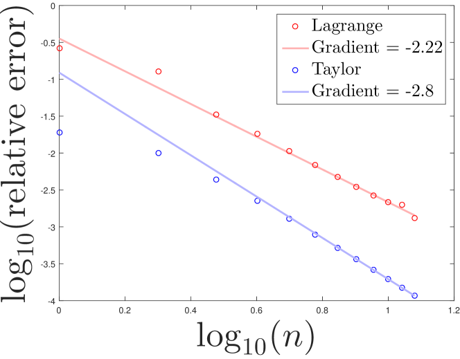
Figure 1: log-log error plot comparison between the Lagrange interpolation and Taylor methods for Example 1. The gradient of each solid line is given by a linear regression on the last 5 points.

We see that both methods achieve the expected quadratic convergence rate. In this simple example, the convergence is quite smooth and the Taylor method performs better than the Lagrange interpolation method.

4.2 Example 2

We implement an example where the coefficients are not uniformly elliptic and $\displaystyle N=d=2$. We write $\displaystyle X_{t}^{0,x}=\left(X_{t}^{1},X_{t}^{2}\right)$ to lighten notation slightly. The example we consider is

$$\begin{pmatrix}X_{t}^{1}\\ X_{t}^{2}\end{pmatrix}=\begin{pmatrix}x_{1}\\ x_{2}\end{pmatrix}+\int_{0}^{t}\begin{pmatrix}\left[2+\sin\left(\mathbb{E}\,X_{s}^{2}\right)\right]\\ X_{t}^{1}\end{pmatrix}\circ dB^{1}_{s}+\int_{0}^{t}\begin{pmatrix}X_{t}^{2}\\ X_{t}^{1}\end{pmatrix}\circ dB^{2}_{s},$$

where the coefficients are

$$V_{0}\equiv 0,\quad V_{1}(x_{1},x_{2},x^{\prime})=\begin{pmatrix}2+\sin(x^{\prime})\\ x_{1}\end{pmatrix},\quad V_{2}(x_{1},x_{2},x^{\prime})=\begin{pmatrix}x_{2}\\ x_{1}\end{pmatrix},\quad\varphi_{1}(x_{1},x_{2})=x_{2},$$

for all $\displaystyle(x_{1},x_{2},x^{\prime})\in\mathbb{R}^{3}$. We note that at $\displaystyle x_{1}=0$ the coefficients degenerate. Second, we note that

$$V_{[(1,2)]}(x_{1},x_{2},x^{\prime})=\begin{pmatrix}x_{1}\\ 2+\sin(x^{\prime})-x_{1}\end{pmatrix}.$$

Since $\displaystyle x_{1}$ and $\displaystyle 2+\sin(x^{\prime})-x_{1}$ cannot both be zero at the same time, we see that $\displaystyle V_{1},V_{2}$ and $\displaystyle V_{[(1,2)]}$ span $\displaystyle\mathbb{R}^{2}$. The coefficients therefore satisfy Assumption 1.3 (A1), the uniform strong Hörmander condition, for $\displaystyle m=2$. For $\displaystyle m=2$, with a cubature formula of degree 5, we expect to achieve a convergence rate of $\displaystyle 3/2$ according to Theorem 1.4. To do so, we have to choose $\displaystyle\gamma\in(4,5)$ and $\displaystyle r>7/2$. We choose the parameters $\displaystyle(x_{1},x_{2},T,\gamma,r)=(1,0.5,1,4.5,4)$, with the terminal function $\displaystyle f(x)=x^{+}$. We implement the cubature formula of degree 5 in dimension $\displaystyle d=2$ from Lyons & Victoir [24]. In this case, the cubature measure is supported on $\displaystyle N_{Cub}=13$ paths. We could not find an explicit solution, so we compare the cubature approximation to a Monte Carlo approximation with Euler-Maruyama discretisation. The results are presented in Figure 2.

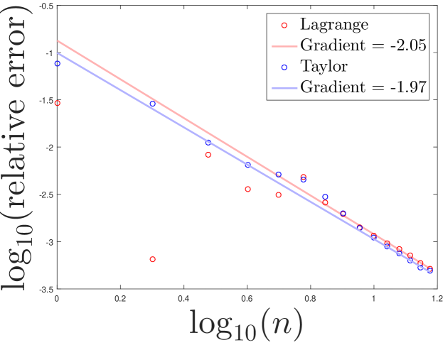
Figure 2: log-log error plot comparison between the Lagrange interpolation and Taylor methods for Example 2. The gradient of each solid line is given by a linear regression on the last 5 points.

In this example, the convergence is not as smooth as Example 1, but the $\displaystyle\log$-$\displaystyle\log$ error plot looks approximately linear after 7 steps. After this, the performance of each algorithm is remarkably similar. Empirically we observe second order convergence, whereas Theorem 1.4 predicts a rate of $\displaystyle 3/2$.

Appendix A Derivative estimates for time-inhomogeneous parabolic PDEs

In this section, we obtain estimates on the derivatives of the solution of the linear parabolic partial differential equation (PDE)

$$\displaystyle\begin{split}\left(\partial_{t}+\mathcal{L}_{t}\right)u(t,x)=0&,\>\>\>\>\>\>(t,x)\in[0,T)\times\mathbb{R}^{N}\\ u(T,x)=f(x)&,\>\>\>\>\>\>x\in\mathbb{R}^{N}\end{split}$$ (A.1)

where $\displaystyle f$ is either Lipschitz or continuous and bounded, and $\displaystyle\mathcal{L}_{t}$ is the time-inhomogeneous differential operator, written in Hörmander form,

$$\mathcal{L}_{t}=W_{0}(t)+\frac{1}{2}\sum_{i=1}^{d}W_{i}(t)^{2}.$$

The connection between parabolic PDEs and stochastic differential equations has been well-studied. Under various types of conditions on the vector fields $\displaystyle W_{0},\ldots,W_{d}$ and terminal condition $\displaystyle f$, the solution to (A.1) is given by $\displaystyle u(t,x)=\mathbb{E}[f(X_{T}^{t,x})]$, where $\displaystyle(X^{t,x}_{s})_{s\in[t,T]}$ solves the following Stratonovich SDE driven by a Brownian motion $\displaystyle B=(B^{1},\ldots,B^{d})$, with the convention $\displaystyle B^{0}_{t}=t$,

$$X_{s}^{t,x}=x+\sum_{i=0}^{d}\int_{t}^{s}W_{i}(u,X_{u}^{t,x})\circ dB^{i}_{u}.$$ (A.2)

In the homogeneous case, Kusuoka & Stroock [20] under a uniform Hörmander condition and subsequently Kusuoka [19] under the weaker UFG condition, establish sharp estimates on the derivatives of the solution of (A.1). Crisan & Delarue [5] extend this analysis to semi-linear equations. To our knowledge, these results have not been obtained without using Malliavin Calculus.

When the vector fields defining the time-inhomogeneous SDE are smooth in time and space, we can consider the space-time process $\displaystyle\left(t,X_{t}^{0,x}\right)_{t\in[0,T]}$ on $\displaystyle\mathbb{R}^{N+1}$ and adapt existing results in the literature. There are three main works we draw on: we first show how to adapt the results of Kusuoka [19] to derive gradient bounds in the directions of the vector fields except $\displaystyle W_{0}$; we then adapt an argument from Crisan & Delarue [5] to prove that the time-inhomogeneous semigroup is a generalised classical solution to a parabolic PDE, and finally using this PDE as a tool, we adapt a result from Crisan, Manolarakis & Nee [10] to derive gradient bounds in the direction of all the vector fields, including $\displaystyle W_{0}$.

We introduce the first assumption which we make throughout this section.

Assumption A.1.

$\displaystyle W_{0},\ldots,W_{d}\in\mathcal{C}^{\infty}_{b}([0,T]\times\mathbb{R}^{N};\mathbb{R}^{N})$.

Under this assumption, (A.2) has a unique strong solution. Now, let us define the space-time process $\displaystyle\left(\widetilde{X}^{(t,x)}_{s}\right)_{s\in[t,T]}:=\left(s,X^{t,x}_{s}\right)_{s\in[t,T]}$, taking values in $\displaystyle\mathbb{R}^{N+1}$, which solves the equation

$$\widetilde{X}^{(t,x)}_{s}=\begin{pmatrix}t\\ x\end{pmatrix}+\int_{t}^{s}\begin{pmatrix}1\\ W_{0}\left(\widetilde{X}^{(t,x)}_{u}\right)\end{pmatrix}\,du+\sum_{i=1}^{d}\int_{t}^{s}\begin{pmatrix}0\\ W_{i}\left(\widetilde{X}^{(t,x)}_{u}\right)\end{pmatrix}\circ dB^{i}_{u}.$$ (A.3)

Defining $\displaystyle\widetilde{x}:=(t,x)\in\mathbb{R}^{N+1}$ and $\displaystyle\widetilde{W}_{0},\ldots,\widetilde{W}_{d}:\mathbb{R}^{N+1}\to\mathbb{R}^{N+1}$ as follows:

$$\displaystyle\forall\widetilde{x}\in\mathbb{R}^{N+1}:\quad\widetilde{W}_{0}(\widetilde{x}):=\begin{pmatrix}1\\ W_{0}(\widetilde{x})\end{pmatrix},\quad\widetilde{W}_{i}(\widetilde{x}):=\begin{pmatrix}0\\ W_{i}(\widetilde{x})\end{pmatrix}\>\text{ for }i=1,\ldots,d,$$

we can re-write (A.3) more compactly as

$$\widetilde{X}^{\widetilde{x}}_{s}=\widetilde{x}+\sum_{i=0}^{d}\int_{t}^{s}\widetilde{W}_{i}\left(\widetilde{X}^{\widetilde{x}}_{u}\right)\circ dB^{i}_{u}.$$ (A.4)

As we shall see, by working under the relaxed $\displaystyle\widetilde{UFG}$ condition (see Assumption A.2), the solution of the PDE (A.1) is not necessarily differentiable in each co-ordinate direction in $\displaystyle\mathbb{R}^{N}$. The solution of (A.1) remains differentiable in certain directions, determined by the vector fields $\displaystyle\widetilde{W}_{0},\ldots,\widetilde{W}_{d}$. We now explain what we mean by such a directional derivative.

We can identify vector fields, $\displaystyle U:\mathbb{R}^{m}\to\mathbb{R}^{m}$ with differential operators acting on sufficiently smooth functions $\displaystyle\varphi:\mathbb{R}^{m}\to\mathbb{R}$ by

$$\forall y\in\mathbb{R}^{m}:\quad U\varphi(y):=\nabla\varphi(y)\,U(y)=\sum_{i=1}^{m}U^{i}(y)\,\partial_{y_{i}}\varphi(y)$$ (A.5)

We can define a directional derivative of $\displaystyle\varphi$ in the direction $\displaystyle U$, even when $\displaystyle\partial_{y_{j}}\varphi$ does not exist classically for all $\displaystyle j=1,\ldots,m$. Let $\displaystyle w_{s}(y)$ be the solution to the ODE

$$\displaystyle\begin{split}&\frac{dw_{s}(y)}{ds}=U(w_{s}(y)),\quad s\geq 0\\ &w_{0}(y)=y.\end{split}$$ (A.6)

We say that $\displaystyle\varphi$ is differentiable in the direction $\displaystyle U$ if the function $\displaystyle s\mapsto\varphi(w_{s}(y))$ is differentiable at 0. Then, we denote

$$U\varphi(y)=\left.\frac{d}{ds}\varphi(w_{s}(y))\right|_{s=0},$$

which coincides with (A.5) when $\displaystyle\varphi\in\mathcal{C}^{1}(\mathbb{R}^{m};\mathbb{R})$. In fact, we will see that the semigroup associated to equation is differentiable in directions determined by commutators of the vector fields. The Lie bracket, or commutator, between two vector fields $\displaystyle U$ and $\displaystyle W$ is then defined the differential operator

$$[U,W]\varphi:=U(W\varphi)-W(U\varphi),$$

which can be identified with the vector field

$$[U,W](y)=\partial W(y)U(y)-\partial U(y)W(y),$$

where $\displaystyle\partial W(y):=(\partial_{y_{j}}W^{i}(y))_{1\leq i,j\leq m}$ is the Jacobian matrix of $\displaystyle W$ and similarly for $\displaystyle\partial U$.

Since we have assumed the vector fields $\displaystyle\widetilde{W}_{0},\ldots,\widetilde{W}_{d}$ to be smooth, we can repeatedly take commutators of them. Recall the notation $\displaystyle\mathcal{A}$ for multi-indices on $\displaystyle\{0,\ldots,d\}$ from section LABEL:sec:introCub. We define $\displaystyle\widetilde{W}_{[\alpha]}$, for $\displaystyle\alpha\in\mathcal{A}$ inductively by forming Lie brackets on $\displaystyle\mathbb{R}^{N+1}$:

$$\displaystyle\widetilde{W}_{[i]}:=\widetilde{W}_{i},\>\>\>\>\>\widetilde{W}_{[\alpha*i]}:=[\widetilde{W}_{[\alpha]},W_{i}]\>\>\>\text{ for }\>i=0\ldots,d,\>\>\alpha\in\mathcal{A}.$$

We note that for all $\displaystyle\alpha\in\mathcal{A}_{1}(m)$ (i.e. for $\displaystyle\alpha\neq(0)$) the first component of the vector field $\displaystyle\widetilde{W}_{[\alpha]}$ is zero. So for $\displaystyle\alpha\in\mathcal{A}_{1}(m)$, a derivative in the direction $\displaystyle\widetilde{W}_{[\alpha]}$ of a function $\displaystyle\mathbb{R}^{N+1}\ni(t,x)\mapsto\phi(t,x)\in\mathbb{R}$ only acts in the $\displaystyle x$ variable. We can therefore write $\displaystyle\{\widetilde{W}_{[\alpha]}(t):\alpha\in\mathcal{A}_{1}(m)\}$ and think of these as differential operators parametrised by $\displaystyle t$ and acting in the $\displaystyle x$ variable. Only the vector field $\displaystyle\\ widetilde{W}_{0}$ acts in the $\displaystyle t$-direction.

With these concepts in mind, we can now introduce the second assumption we make on the vector fields.

Assumption A.2.

$\displaystyle\widetilde{UFG}$($\displaystyle m$) condition: there exists a positive integer $\displaystyle m$ such that, for all $\displaystyle\alpha\in\mathcal{A}$ with $\displaystyle\|\alpha\|>m$, there exist $\displaystyle\varphi_{\alpha,\beta}\in\mathcal{C}_{b}^{\infty}([0,T]\times\mathbb{R}^{N};\mathbb{R})$ with

$$\widetilde{W}_{[\alpha]}(t,x)=\sum_{\beta\in\mathcal{A}_{1}(m)}\varphi_{\alpha,\beta}(t,x)\,\widetilde{W}_{[\beta]}(t,x).$$

A.1 Kusuoka-Stroock processes

This class of process was introduced by Kusuoka & Stroock [21]. They will appear as Malliavin weights in our integration by parts formulas. The definition and properties we give here record the regularity and growth of these processes with respect to different parameters. The results allow one to develop integration by parts formulas in a systematic and transparent way, which automatically leads to nice derivative estimates.

Definition A.3 (Kusuoka-Stroock processes).

Let $\displaystyle E$ be a separable Hilbert space and let $\displaystyle r\in\mathbb{R}$, $\displaystyle M\in\mathbb{N}$. We denote by $\displaystyle\mathcal{K}_{r}(t,E,M)$ the set of functions: $\displaystyle\Phi_{t}:(t,T]\times\mathbb{R}^{N}\to\mathbb{D}^{M,\infty}(E)$ satisfying the following:

1. For all $\displaystyle s\in(t,T]$, the map $\displaystyle\mathbb{R}^{N}\ni x\mapsto\Phi_{t}(s,x)\in L^{p}(\Omega)$ is $\displaystyle M$-times continuously differentiable for all $\displaystyle p\geq 1$.

2. For any $\displaystyle p\geq 1$, any multi-index $\displaystyle\alpha$ on $\displaystyle\{1,\ldots,N\}$ and $\displaystyle m\in\mathbb{N}$ with $\displaystyle|\alpha|+m\leq M$, we have

   $$\displaystyle\begin{split}\sup_{x\in\mathbb{R}^{N}}\sup_{s\in(t,T]}(s-t)^{-r/2}&\left\|\partial^{\alpha}_{x}\Phi_{t}(s,x)\right\|_{\mathbb{D}^{m,p}(E)}<\infty.\end{split}$$ (A.7)

Remark A.4.

1. The number $\displaystyle M$ denotes how many times the Kusuoka-Stroock function can be differentiated and $\displaystyle r$ measures the growth in $\displaystyle(s-t)$.

2. This definition is slightly different to that in [21]: here our processes are defined on $\displaystyle(t,T]$ instead of $\displaystyle(0,T]$ and we require continuity in $\displaystyle L^{p}(\Omega)$ rather than almost surely.

We record here some properties which help when building Malliavin weights later.

Lemma A.5.

1. If $\displaystyle\Phi_{t}\in\mathcal{K}^{q}_{r}(t,\mathbb{R},M)$ is $\displaystyle\mathbb{F}$-adapted, and we define
   $\displaystyle\textstyle\Psi^{i}_{t}(s,x):=\int_{t}^{s}\Phi_{t}(u,x)\,dB^{i}_{u}$ for $\displaystyle i\in\{1,\ldots,d\}$ and $\displaystyle\textstyle\Gamma(s,x):=\int_{t}^{s}\Phi_{t}(u,x)\,du$, then $\displaystyle\Psi_{t}^{i}\in\mathcal{K}^{q}_{r+1}(t,\mathbb{R},M)$ and $\displaystyle\Gamma_{t}\in\mathcal{K}^{q}_{r+2}(t,\mathbb{R},M)$.

2. If $\displaystyle\Phi_{t,i}\in\mathcal{K}^{q_{i}}_{r_{i}}(t,\mathbb{R},M_{i}),i=1,\ldots,n$ then $\displaystyle\textstyle\sum_{i=1}^{n}\Phi_{t,i}\in\mathcal{K}^{\max_{i}q_{i}}_{\min_{i}r_{i}}(t,\mathbb{R},\min_{i}M_{i})$ and
   $\displaystyle\textstyle\prod_{i=1}^{n}\Phi_{t,i}\in\mathcal{K}^{q_{1}+\ldots+q_{n}}_{r_{1}+\ldots+r_{N}}(t,\mathbb{R},\min_{i}M_{i})$.

Proof.

The proof is essentially the same as the proof of Lemma 75 in [10]. ∎

A.2 Integration by parts & derivative bounds

We are now in a position to prove the main integration by parts result.

Theorem A.6.

Assume that $\displaystyle\widetilde{UFG}(m)$ holds and fix $\displaystyle s\in(t,T]$. Then, for any $\displaystyle\alpha_{1},\ldots,\alpha_{n}\in\mathcal{A}_{1}(m)$, there exist $\displaystyle\Phi^{1}_{t,\alpha_{1},\ldots,\alpha_{n}}\in\mathcal{K}_{0}(t,\mathbb{R})$ and $\displaystyle\Phi^{2}_{t,\alpha_{1},\ldots,\alpha_{n}}\in\mathcal{K}_{0}(t,\mathbb{R}^{N})$ such that for $\displaystyle f\in\mathcal{C}^{\infty}_{b}(\mathbb{R}^{N};\mathbb{R})$,

$$\widetilde{W}_{[\alpha_{1}]}(t)\cdots\widetilde{W}_{[\alpha_{n}]}(t)\left(P_{t,s}f\right)(x)=(s-t)^{-\frac{\|\alpha_{1}\|+\ldots,+\|\alpha_{n}\|}{2}}\mathbb{E}\left[f(X_{s}^{t,x})\,\Phi^{1}_{t,\alpha_{1},\ldots,\alpha_{n}}(s,x)\right],$$ (A.8)

and

$$\widetilde{W}_{[\alpha_{1}]}(t)\cdots\widetilde{W}_{[\alpha_{n}]}(t)\left(P_{t,s}f\right)(x)=(s-t)^{-\frac{\|\alpha_{1}\|+\ldots,+\|\alpha_{n-1}\|}{2}}\mathbb{E}\left[\nabla f(X_{s}^{t,x})\,\Phi^{2}_{t,\alpha_{1},\ldots,\alpha_{n}}(s,x)\right].$$ (A.9)

Moreover, for $\displaystyle f$ continuous and bounded or Lipschitz, $\displaystyle P_{t,s}f(x)$ is differentiable in the directions $\displaystyle\{\widetilde{W}_{[\alpha]}(t):\alpha\in\mathcal{A}_{1}(m)\}$ with

$$\sup_{x\in\mathbb{R}^{N}}\left|\widetilde{W}_{[\alpha_{1}]}(t)\cdots\widetilde{W}_{[\alpha_{n}]}(t)\left(P_{t,s}f\right)(x)\right|\leq C\,\|f\|_{\infty}\,(s-t)^{\frac{-(|\alpha_{1}|+\ldots,+|\alpha_{n}|)}{2}},$$ (A.10)

and

$$\sup_{x\in\mathbb{R}^{N}}\left|\widetilde{W}_{[\alpha_{1}]}(t)\cdots\widetilde{W}_{[\alpha_{n}]}(t)\left(P_{t,s}f\right)(x)\right|\leq C\,\|f\|_{\text{Lip}}\,(s-t)^{\frac{1-(|\alpha_{1}|+\ldots,+|\alpha_{n}|)}{2}},$$ (A.11)

in each case, respectively.

Remark A.7.

We emphasise here that each $\displaystyle\widetilde{W}_{[\alpha_{1}]}(t)$ is a differential operator acting in $\displaystyle x$, parametrised by $\displaystyle t$, applied to the function $\displaystyle x\mapsto P_{t,s}f(x)$. These results are not valid for e.g. $\displaystyle\widetilde{W}_{[\alpha_{1}]}(u)P_{t,s}f(x)$ when $\displaystyle u\neq t$. We develop estimates on the derivative of $\displaystyle(t,x)\mapsto P_{t,s}f(x)$ as a function on $\displaystyle[0,T]\times\mathbb{R}^{N}$ in Proposition A.14.

Proof of Theorem A.6.

Since the $\displaystyle\widetilde{UFG}$ condition is precisely the UFG condition of Kusuoka on $\displaystyle\mathbb{R}^{N+1}$, we can use his results. We use the notation $\displaystyle\widetilde{P}_{s}g(\widetilde{x}):=\mathbb{E}\left[g\left(\widetilde{X}^{\widetilde{x}}_{s}\right)\right]$ for a suitably integrable function $\displaystyle g:\mathbb{R}^{N+1}\to\mathbb{R}$. By Kusuoka [19] Lemma 8 (see also [10] Corollary 32), we know for any $\displaystyle\alpha_{1},\ldots,\alpha_{n}\in\mathcal{A}_{1}(m)$, there exist $\displaystyle\Phi^{1}_{\alpha_{1},\ldots,\alpha_{n}}\in\mathcal{K}_{0}(\mathbb{R})$ and $\displaystyle\Phi^{2}_{\alpha_{1},\ldots,\alpha_{n}}\in\mathcal{K}_{0}(\mathbb{R}^{N+1})$ such that for $\displaystyle g\in\mathcal{C}^{\infty}_{b}(\mathbb{R}^{N+1};\mathbb{R})$,

$$\widetilde{W}_{[\alpha_{1}]}(t)\cdots\widetilde{W}_{[\alpha_{n}]}(t)\left(\widetilde{P}_{s}g\right)(\widetilde{x})=(s-t)^{-\frac{\|\alpha_{1}\|+\ldots,+\|\alpha_{n}\|}{2}}\mathbb{E}\left[g(\widetilde{X}_{s}^{\widetilde{x}})\,\Phi^{1}_{\alpha_{1},\ldots,\alpha_{n}}(s,\widetilde{x})\right],$$

and

$$\widetilde{W}_{[\alpha_{1}]}(t)\cdots\widetilde{W}_{[\alpha_{n}]}(t)\left(\widetilde{P}_{s}g\right)(\widetilde{x})=(s-t)^{-\frac{\|\alpha_{1}\|+\ldots,+\|\alpha_{n-1}\|}{2}}\mathbb{E}\left[\nabla g(\widetilde{X}_{s}^{\widetilde{x}})\,\Phi^{2}_{\alpha_{1},\ldots,\alpha_{n}}(s,\widetilde{x})\right].$$

Now for any function $\displaystyle f\in\mathcal{C}^{\infty}_{b}(\mathbb{R}^{N};\mathbb{R})$, we can extend it to $\displaystyle g\in\mathcal{C}^{\infty}_{b}(\mathbb{R}^{N+1};\mathbb{R})$ by $\displaystyle g(t,x):=f(x)$. We then immediately have the integration by parts formulas (A.8) and (A.9). We get the bound stated in (A.10) with the constant

$$C=\sup_{s\in[t,T]}\sup_{x\in\mathbb{R}^{N}}\mathbb{E}\left|\Phi^{1}_{t,\alpha_{1},\ldots,\alpha_{n}}(s,x)\right|,$$

and a standard approximation argument gives the same estimate for bounded and continuous $\displaystyle f$. Similarly, we obtain the bound in (A.11) with constant

$$C=\sup_{s\in[t,T]}\sup_{x\in\mathbb{R}^{N}}\mathbb{E}\left|\Phi^{2}_{t,\alpha_{1},\ldots,\alpha_{n}}(s,x)\right|,$$

and a standard approximation argument allows one to obtain the same bound for $\displaystyle f$ Lipschitz with $\displaystyle\|\nabla f\|_{\infty}$ replaced by $\displaystyle\|f\|_{Lip}$. ∎

A.3 Uniform Hörmander setting

In this section, let us consider a stronger assumption than the $\displaystyle\widetilde{UFG}(m)$ condition. Suppose that a uniform strong Hörmander condition of order $\displaystyle m$ holds - that is

Assumption A.8.

USH($\displaystyle m$) : There exists $\displaystyle\delta>0$ and $\displaystyle m\in\mathbb{N}$ such that for all $\displaystyle\xi\in\mathbb{R}^{N}$,

$$\inf_{(t,z)\in[0,T]\times\mathbb{R}^{N}}\sum_{\alpha\in\mathcal{A}_{\geq 1}(m)}\langle W_{[\alpha]}(t,z),\xi\rangle^{2}\geq\delta\,|\xi|^{2}.$$

In this case, we recover differentiability of $\displaystyle x\mapsto P_{t,T}f(x)$ in all directions.

Corollary A.9.

Assume USH($\displaystyle m$) holds. Let $\displaystyle\eta$ be a multi-index on $\displaystyle\{1,\ldots,N\}$ and let $\displaystyle f$ be Lipschitz. Then,

$$\sup_{x\in\mathbb{R}^{N}}\left|\partial^{\eta}\left(P_{t,T}f\right)(x)\right|\leq C\,\|f\|_{Lip}\,(T-t)^{-(|\eta|-1)m/2}.$$

Proof.

First let $\displaystyle f\in\mathcal{C}^{\infty}_{b}(\mathbb{R}^{N};\mathbb{R})$. For the first order derivatives,

$$\displaystyle\partial^{i}_{x}\mathbb{E}\left[f(X^{t,x}_{T})\right]=\sum_{k=1}^{N}\mathbb{E}\left[\partial^{k}f(X^{t,x}_{T})\,\partial^{i}_{x}(X^{t,x}_{T})^{k}\right].$$

For the higher order derivatives, we note that there exist $\displaystyle F^{i}_{\alpha}\in\mathcal{C}^{\infty}_{b}([0,T]\times\mathbb{R}^{N};\mathbb{R})$ such that

$$e_{j}=\sum_{\alpha\in\mathcal{A}_{\geq 1}(m)}F^{j}_{\alpha}(t,x)\,W_{[\alpha]}(t,x),$$

where $\displaystyle e_{j}$ is the $\displaystyle j$-th standard basis vector in $\displaystyle\mathbb{R}^{N}$. To see this, define $\displaystyle\mathcal{W}(t,x)$ to be the $\displaystyle N\times\text{card}(\mathcal{A}_{\geq 1}(m))$ matrix whose columns are the vector fields $\displaystyle(W_{[\alpha]})_{\alpha\in\mathcal{A}_{\geq 1}(m)}$ evaluated at $\displaystyle(t,x)$. USH($\displaystyle m$) guarantees that $\displaystyle\mathcal{W}\mathcal{W}^{\top}(t,x)$ is invertible. Then,

$$F^{j}_{\alpha}(t,x):=\left(\mathcal{W}^{\top}[\mathcal{W}\mathcal{W}^{\top}]^{-1}(t,x)\,e_{j}\right)_{\alpha}$$

satisfies the above relation. Then, for the second order derivatives,

$$\displaystyle\partial^{(j,i)}_{x}\mathbb{E}\left[f(X_{T}^{t,x})\right] \displaystyle=\sum_{k=1}^{N}\partial^{j}_{x}\mathbb{E}\left[\partial^{k}f(X^{t,x}_{T})\,\partial^{i}_{x}(X^{t,x}_{T})^{k}\right]$$

$$\displaystyle=\sum_{k=1}^{N}\sum_{\alpha\in\mathcal{A}_{\geq 1}(m)}F^{j}_{\alpha}(t,x)\,W_{[\alpha]}(t)\left(\mathbb{E}\left[\partial^{k}f(X^{t,x}_{T})\,\partial^{i}_{x}(X^{t,x}_{T})^{k}\right]\right).$$

We note that $\displaystyle\partial^{i}_{x}(X^{t,x}_{T})^{k}\in\mathcal{K}_{0}(t,\mathbb{R})$, so we can apply the IBPF in Kusuoka [19] Lemma 8 to obtain the existence of $\displaystyle H_{t,\alpha}\in\mathcal{K}_{0}(t,\mathbb{R})$ such that

$$\displaystyle\partial^{(j,i)}_{x}\mathbb{E}\left[f(X_{T}^{t,x})\right] \displaystyle=\sum_{k=1}^{N}\sum_{\alpha\in\mathcal{A}_{\geq 1}(m)}F^{j}_{\alpha}(t,x)\,(T-t)^{-|\alpha|/2}\,\mathbb{E}\left[\partial^{k}f(X^{t,x}_{T})\,H_{t,\alpha}\left(T,x\right)\right]$$

$$\displaystyle=(T-t)^{-m/2}\sum_{k=1}^{N}\mathbb{E}\left[\partial^{k}f(X^{t,x}_{T})\,\bar{H}_{t,i,j,k}(T,x)\right],$$

where

$$\bar{H}_{t,i,j,k}(T,x):=\sum_{\alpha\in\mathcal{A}_{\geq 1}(m)}(T-t)^{(m-|\alpha|)/2}F^{j}_{\alpha}(t,x)H_{t,\alpha}\left(T,x\right)\in\mathcal{K}_{0}(t,\mathbb{R}),$$

and we have used that for all $\displaystyle\alpha\in\mathcal{A}_{\geq 1}(m)$, $\displaystyle\|\alpha\|=|\alpha|\leq m$. We get the bound:

$$\displaystyle\sup_{x\in\mathbb{R}^{N}}\left|\partial^{(j,i)}_{x}\mathbb{E}\left[f(X_{T}^{t,x})\right]\right|\leq(T-t)^{-m/2}\|\nabla f\|_{\infty}\,\sum_{k=1}^{N}\sup_{x\in\mathbb{R}^{N}}\mathbb{E}\left|\bar{H}_{t,i,j,k}(T,x)\right|.$$

We can iterate this argument as many times as we like. Then we can get the bound for a Lipschitz $\displaystyle f$ using approximation as before. ∎

A.4 Connection with PDE

In this section, we make use of the integration by parts formulae of Theorem A.6 to extend the notion of classical solution to the PDE (A.1) to the case when the solution is not classically differentiable in all directions. The notation and arguments in this section closely follows Crisan & Delarue [5], who provide a similar notion of solution to semilinear PDEs with coefficients which do not depend on time. The idea is very simple: it is a standard result that for a terminal condition $\displaystyle f\in\mathcal{C}^{\infty}_{p}(\mathbb{R}^{N};\mathbb{R})$ the PDE (A.1) has a classical solution. For $\displaystyle f\in\mathcal{C}_{p}(\mathbb{R}^{N};\mathbb{R})$, we consider a sequence of smooth approximations $\displaystyle(f_{l})_{l\geq 1}$ to which we can associate solutions $\displaystyle(v_{l})_{l\geq 1}$ to (A.1). For each $\displaystyle v_{l}$ we can use the integration by parts formula of Theorem A.6 to write the derivatives $\displaystyle W_{i}^{2}(t)v_{l}(t,x)$ in a form which does not depend on any derivatives of $\displaystyle f_{l}$. We then show that the PDE still holds in the limit $\displaystyle l\to\infty$.

We introduce some function spaces we will need to define what we mean by a classical solution. We denote by $\displaystyle\mathbb{B}(0,R)$ the open ball in $\displaystyle\mathbb{R}^{N}$ of radius $\displaystyle R>0$ centred at zero. Let $\displaystyle\phi\in\mathcal{C}^{\infty}_{b}([0,T-1/r]\times\mathbb{B}(0,R);\mathbb{R})$ and define

$$\|\phi\|^{\widetilde{W}_{0},1}_{[0,T-1/R]\times\mathbb{B}(0,R);\infty}:=\|\phi\|_{[0,T-1/R]\times\mathbb{B}(0,R);\infty}+\|\widetilde{W}_{0}(t)\phi\|_{[0,T-1/R]\times\mathbb{B}(0,R);\infty}.$$

Define $\displaystyle\mathcal{D}^{1,\infty}_{\widetilde{W}_{0}}([0,T-1/R]\times\mathbb{B}(0,R))$ as the closure of $\displaystyle\mathcal{C}^{\infty}_{b}([0,T-1/R]\times\mathbb{B}(0,R);\mathbb{R})$ in $\displaystyle\mathcal{C}_{b}([0,T-1/R]\times\bar{\mathbb{B}}(0,R);\mathbb{R})$ with respect to the norm $\displaystyle\|\cdot\|^{\widetilde{W}_{0},1}_{[0,T-1/R]\times\mathbb{B}(0,R);\infty}$. And define

$$\mathcal{D}^{1,\infty}_{\widetilde{W}_{0}}([0,T)\times\mathbb{R}^{N}):=\bigcap_{R\geq 1}\mathcal{D}^{1,\infty}_{\widetilde{W}_{0}}([0,T-1/R]\times\mathbb{B}(0,R)).$$

Now, take $\displaystyle\psi\in\mathcal{C}^{\infty}_{b}(\mathbb{R}^{N};\mathbb{R})$ and, for any ball $\displaystyle\mathbb{B}$, define

$$\|\psi\|^{W(t),1}_{\mathbb{B},\infty}:=\|\psi\|_{\mathbb{B},\infty}+\sum_{i=1}^{d}\|W_{i}(t)\psi\|_{\mathbb{B},\infty},$$

and

$$\|\psi\|^{W(t),2}_{\mathbb{B},\infty}:=\|\psi\|^{W(t),1}_{\mathbb{B},\infty}+\sum_{i=1}^{d}\|W_{i}^{2}(t)\psi\|_{\mathbb{B},\infty}.$$

We define $\displaystyle\mathcal{D}_{W(t)}^{2,\infty}(\mathbb{B})$ to be the closure of $\displaystyle\mathcal{C}^{\infty}_{b}(\mathbb{B};\mathbb{R})$ in $\displaystyle\mathcal{C}_{b}(\bar{\mathbb{B}};\mathbb{R})$ with respect to $\displaystyle\|\cdot\|^{W(t),2}_{\mathbb{B},\infty}$ and

$$\mathcal{D}_{W(t)}^{2,\infty}(\mathbb{R}^{N}):=\bigcap_{R\geq 1}\mathcal{D}_{W(t)}^{2,\infty}(\mathbb{B}(0,R)).$$

Definition A.10 (Classical solution).

We define a function $\displaystyle v:[0,T]\times\mathbb{R}^{N}\to\mathbb{R}$ to be a classical solution to (A.1) if the following three conditions are satisfied:

1. $\displaystyle v\in\mathcal{D}^{1,\infty}_{\widetilde{W}_{0}}([0,T)\times\mathbb{R}^{N})$ and for each $\displaystyle t\in[0,T)$, $\displaystyle v(t,\cdot)\in\mathcal{D}_{W(t)}^{2,\infty}(\mathbb{R}^{N})$, such that for $\displaystyle i=1,\ldots,d$,

   $$[0,T)\times\mathbb{R}^{N}\ni(t,x)\mapsto\left(W_{i}(t)v(t,x),W_{i}^{2}(t)v(t,x)\right)$$

   is a continuous function.

2. For all $\displaystyle(t,x)\in[0,T)\times\mathbb{R}^{N}$,

   $$\widetilde{W}_{0}v(t,x)+\frac{1}{2}\sum_{i=1}^{d}W_{i}^{2}v(t,x)=0$$

3. $\displaystyle\lim_{(t,y)\to(T,x)}v(t,y)=f(x)$ for all $\displaystyle x\in\mathbb{R}^{N}$.

Remark A.11.

1. Note that since, in general, the space $\displaystyle\mathcal{D}_{W(t)}^{2,\infty}(\mathbb{R}^{N})$ is different for each $\displaystyle t\in[0,T)$, our definition requires that $\displaystyle v(t,\cdot)$ belongs to a different space at each time $\displaystyle t\in[0,T)$.

2. If $\displaystyle\phi\in\mathcal{C}^{1,2}([0,T)\times\mathbb{R}^{N};\mathbb{R})$, then $\displaystyle\phi\in\mathcal{D}^{1,\infty}_{\widetilde{W}_{0}}([0,T)\times\mathbb{R}^{N})$ and $\displaystyle\phi(t,\cdot)\in\mathcal{D}_{W(t)}^{2,\infty}(\mathbb{R}^{N})$ for all $\displaystyle t\in[0,T)$. Moreover,

   $$\displaystyle\|\phi\|^{\widetilde{W}_{0},1}_{[0,T-1/R]\times\mathbb{B}(0,r);\infty} \displaystyle\leq C_{R}\,\big{\{}\|\phi\|_{[0,T-1/r]\times\mathbb{B}(0,r);\infty}+\|\partial_{t}\phi\|_{[0,T-1/R]\times\mathbb{B}(0,R);\infty}$$

   $$\displaystyle\quad\quad\quad+\|\nabla\phi\|_{[0,T-1/R]\times\mathbb{B}(0,R);\infty}\big{\}}$$

   $$\displaystyle\|\phi\|^{W(t),2}_{\mathbb{B}(0,R),\infty} \displaystyle\leq C_{R}\left\{\|\phi(t,\cdot)\|_{\mathbb{B}(0,R);\infty}+\|\nabla\phi(t,\cdot)\|_{\mathbb{B}(0,R);\infty}+\|\nabla^{2}\phi(t,\cdot)\|_{\mathbb{B}(0,R);\infty}\right\},$$

   where

   $$\displaystyle C_{R}=1+\|W_{0}\|_{[0,T-1/R]\times\mathbb{B}(0,R);\infty}+\sum_{i=1}^{d}\|W_{i}(t,\cdot)\|_{\mathbb{B}(0,R);\infty}+\|\partial W_{i}(t,\cdot)\|_{\mathbb{B}(0,R);\infty}.$$

   It is then clear that our definition truly is an extension of the usual definition of classical solution.

With this definition in hand, we have the following theorem.

Theorem A.12.

Assume that $\displaystyle\widetilde{UFG}(m)$ holds and let $\displaystyle f:\mathbb{R}^{N}\to\mathbb{R}$ be continuous with polynomial growth. Then, $\displaystyle v(t,x):=P_{t,T}f(x)$ is a classical solution to (A.1). It is also the unique solution amongst those which satisfy the following polynomial growth condition: there exists $\displaystyle q>0$ such that

$$\left|v(t,x)\right|\leq C(1+|x|)^{q}\quad\forall t\in[0,T],x\in\mathbb{R}^{N}$$

The proof of uniqueness relies on an Itô formula valid for functions differentiable in the directions of the vector fields. We will also need a stochastic Taylor expansion based on this formula in Section A.6 for the analysis of the error in the cubature on Wiener space algorithm.

Lemma A.13.

Let $\displaystyle v:[0,T)\times\mathbb{R}^{N}\to\mathbb{R}$ satisfy part (1) of Definition A.10 and be of at most polynomial growth. Then, for all $\displaystyle u\in[t,T)$,

$$\displaystyle\begin{split}v(u,X^{t,x}_{u})=v(t,x)+\int_{t}^{u}&\left[\widetilde{W}_{0}(s)v(s,X_{s}^{t,x})+\frac{1}{2}\sum_{i=1}^{d}W_{i}^{2}(s)v(s,X_{s}^{t,x})\right]ds\\ &+\sum_{i=1}^{d}\int_{t}^{u}W_{i}(s)v(s,X_{s}^{t,x})dB^{i}_{s}.\end{split}$$ (A.12)

Proof.

This can be proved by a mollification argument as in Proposition 7.1 in [5]. ∎

We can now prove Theorem A.12.

Proof of Theorem A.12.

Existence: Denote by $\displaystyle(f_{l})_{l\geq 1}$ a sequence of mollifications of $\displaystyle f$. Since $\displaystyle f$ is continuous, $\displaystyle f_{l}$ converges to $\displaystyle f$ uniformly on compact subsets of $\displaystyle\mathbb{R}^{N}$. Since $\displaystyle v_{l}(t,x)-v(t,x)=\mathbb{E}\left[f_{l}(X^{t,x}_{T})-f(X^{t,x}_{T})\right]$, it is clear that $\displaystyle v_{l}$ converges to $\displaystyle v$ uniformly on compact subsets of $\displaystyle[0,T]\times\mathbb{R}^{N}$. Therefore, $\displaystyle v$ is continuous up to the boundary at $\displaystyle t=T$. Now, consider the integration by parts formula for $\displaystyle W_{i}v_{l}$ and $\displaystyle W_{i}^{2}v_{l}$ provided by (A.8) as part of Theorem A.6. We get

$$\displaystyle W_{i}v_{l}(t,x)=(T-t)^{-1/2}\,\mathbb{E}\left[f_{l}(X_{T}^{t,x})\Phi^{1}_{t,(i)}(T,x)\right],$$

$$\displaystyle W_{i}^{2}v_{l}(t,x)=(T-t)^{-1}\,\mathbb{E}\left[f_{l}(X_{T}^{t,x})\Phi^{1}_{t,(i,i)}(T,x)\right],$$

where, crucially, $\displaystyle\Phi^{1}_{t,(i)},\Phi^{1}_{t,(i,i)}$ are independent of $\displaystyle f_{l}$. Then, considering the differences $\displaystyle W_{i}v_{l}(t,x)-W_{i}v_{m}(t,x)$ and $\displaystyle W_{i}^{2}v_{l}(t,x)-W_{i}^{2}v_{m}(t,x)$ over compact subsets of $\displaystyle[0,T)\times\mathbb{R}^{N}$, we see that $\displaystyle(W_{i}v_{l},W_{i}^{2}v_{l})_{l\geq 1}$ converges uniformly on compact subsets of $\displaystyle[0,T)\times\mathbb{R}^{N}$. This proves that $\displaystyle W_{i}v,W_{i}^{2}v$ exist and are continuous. Now, each $\displaystyle f_{l}\in\mathcal{C}_{p}^{\infty}(\mathbb{R}^{N};\mathbb{R})$, so associated to each, there is a classical solution $\displaystyle v_{l}$ of the PDE (A.1). Since $\displaystyle\widetilde{W}_{0}v_{l}=\textstyle-\frac{1}{2}\sum_{i=1}^{d}W_{i}^{2}v_{l}$, and $\displaystyle W_{i}^{2}v_{l}\to W_{i}^{2}v$ uniformly on compacts in $\displaystyle[0,T)\times\mathbb{R}^{N}$, we get that $\displaystyle v\in\mathcal{D}^{1,\infty}_{\widetilde{W}_{0}}([0,T)\times\mathbb{R}^{N})$. Moreover, taking the limit in the PDE satisfied by $\displaystyle v_{l}$ shows that it is also satisfied by $\displaystyle v$.

Uniqueness: Using the Itô formula in Lemma A.13, we have for $\displaystyle u<T$

$$\displaystyle v(u,X^{t,x}_{u})=v(t,x) \displaystyle+\int_{t}^{u}\left[\widetilde{W}_{0}(s)v(s,X_{s}^{t,x})+\frac{1}{2}\sum_{i=1}^{d}W_{i}^{2}(s)v(s,X_{s}^{t,x})\right]ds$$

$$\displaystyle+\sum_{i=1}^{d}\int_{t}^{u}W_{i}(s)v(s,X_{s}^{t,x})dB^{i}_{s}.$$

Using part (2) of the definition, the drift term is zero and

$$v(u,X^{t,x}_{u})=v(t,x)+\sum_{i=1}^{d}\int_{t}^{u}W_{i}(s)v(s,X_{s}^{t,x})dB^{i}_{s}.$$ (A.13)

Now, using that $\displaystyle v$ has polynomial growth and $\displaystyle X_{u}^{t,x}$ has moments of all orders, we can easily show that the left hand side of (A.13) is square integrable, and so the right hand side is too. Hence the right hand side is a true martingale and we can take expectation in (A.13) to get

$$\mathbb{E}v(u,X^{t,x}_{u})=v(t,x)$$

and using part (3) of the definition (continuity of $\displaystyle v$ at the boundary $\displaystyle t=T$) we can take $\displaystyle u\nearrow T$ to get

$$\mathbb{E}f(X^{t,x}_{T})=v(t,x),$$

which proves uniqueness. ∎

A.5 Derivatives in the direction $\displaystyle\widetilde{W}_{0}$

In Theorem A.6, we established integration by parts formulae for derivatives of $\displaystyle x\mapsto P_{t,T}f(x)$ in the directions $\displaystyle\{\widetilde{W}_{[\alpha]}(t),\alpha\in\mathcal{A}_{1}(m)\}$. However $\displaystyle 0\notin\mathcal{A}_{1}(m)$, so we have no control over derivatives in the direction $\displaystyle\widetilde{W}_{0}$. Using that $\displaystyle P_{t,T}f(x)$ solves PDE (A.1) we are now able to estimate derivatives in the $\displaystyle\widetilde{W}_{0}$ direction.

Proposition A.14.

Assume $\displaystyle\widetilde{UFG}(m)$ holds. Let $\displaystyle\alpha=(\alpha_{1},\ldots,\alpha_{n})\in\mathcal{A}$ and use the notation $\displaystyle\widetilde{W}_{\alpha}(t)=\widetilde{W}_{\alpha_{1}}(t)\cdots\widetilde{W}_{\alpha_{n}}(t)$. Then, the function $\displaystyle v(t,x):=P_{t,T}f(x)$ is differentiable in the directions $\displaystyle\widetilde{W}_{0}(t),W_{1}(t),\ldots,W_{d}(t)$ and the following bounds hold for all $\displaystyle t\in[0,T)$: for $\displaystyle f$ continuous and bounded,

$$\sup_{x\in\mathbb{R}^{N}}\left|\widetilde{W}_{\alpha}(t)v(t,x)\right|\leq C\,\|f\|_{\infty}\,(T-t)^{\frac{-(\|\alpha_{1}\|+\ldots,+\|\alpha_{n}\|)}{2}}.$$ (A.14)

For $\displaystyle f$ Lipschitz,

$$\sup_{x\in\mathbb{R}^{N}}\left|\widetilde{W}_{\alpha}(t)v(t,x)\right|\leq C\,\|f\|_{\text{Lip}}\,(T-t)^{\frac{1-(\|\alpha_{1}\|+\ldots,+\|\alpha_{n}\|)}{2}}.$$ (A.15)

Proof.

Thinking of the $\displaystyle\widetilde{W}_{0},W_{1},\ldots,W_{d}$ as differential operators acting on functions in
$\displaystyle\mathcal{C}^{\infty}([0,T]\times\mathbb{R}^{N};\mathbb{R})$, Corollary 78 in [10] shows that $\displaystyle\widetilde{W}_{\alpha}$, $\displaystyle\alpha\in\mathcal{A}$ satisfies the following convenient identity

$$\widetilde{W}_{\alpha}v=\sum_{i=1}^{\|\alpha\|}\sum_{\begin{subarray}{c}\beta_{1},\ldots,\beta_{i}\in\mathcal{A}_{1},\\ \|\beta_{1}\|+\ldots+\|\beta_{i}\|=\|\alpha\|\end{subarray}}c_{\alpha,\beta_{1},\ldots,\beta_{i}}\widetilde{W}_{[\beta_{1}]}...\widetilde{W}_{[\beta_{i}]}v,$$ (A.16)

where $\displaystyle c_{\alpha,\beta_{1},\ldots,\beta_{i}}\in\mathbb{R}$. The importance of this identity is that the left hand side contains derivatives possibly in the direction $\displaystyle\widetilde{W}_{0}$ whereas on the right hand side, there are only derivatives in directions $\displaystyle\widetilde{W}_{[\alpha]}$, $\displaystyle\alpha\in\mathcal{A}_{1}$ which does not include $\displaystyle\widetilde{W}_{0}$.

Hence,

$$\left|\widetilde{W}_{\alpha}v\right|\leq C\,\sup_{\begin{subarray}{c}\beta_{1},\ldots,\beta_{i}\in\mathcal{A}_{1},\\ \|\beta_{1}\|+\ldots+\|\beta_{i}\|=\|\alpha\|\end{subarray}}\left|\widetilde{W}_{[\beta_{1}]}...\widetilde{W}_{[\beta_{i}]}v\right|,$$

this being exactly the type of term we can control by Theorem A.6. ∎

Now, define, for $\displaystyle\varphi\in\mathcal{C}^{\infty}_{b}([0,T-1/R]\times\mathbb{B}(0,R);\mathbb{R})$, the norm

$$\|\varphi\|^{W,n}_{[0,T-1/R]\times\mathbb{B}(0,R);\infty}:=\sum_{\alpha\in\mathcal{A}(n)}\|\widetilde{W}_{\alpha}\varphi\|_{[0,T-1/R]\times\mathbb{B}(0,R);\infty},$$

and define $\displaystyle\widehat{\mathcal{D}}^{n}([0,T-1/R]\times\mathbb{B}(0,R))$ as the closure of $\displaystyle\mathcal{C}^{\infty}_{b}([0,T-1/R]\times\mathbb{B}(0,R);\mathbb{R})$ in $\displaystyle\mathcal{C}_{b}([0,T-1/R]\times\bar{\mathbb{B}}(0,R);\mathbb{R})$ with respect to this norm. Then, set

$$\widehat{\mathcal{D}}^{\infty}([0,T)\times\mathbb{R}^{N}):=\bigcap_{R\geq 1,n\geq 1}\widehat{\mathcal{D}}^{n}([0,T-1/R]\times\mathbb{B}(0,R)).$$

Lemma A.15.

The function $\displaystyle v(t,x):=P_{t,T}f(x)$ is a member of $\displaystyle\widehat{\mathcal{D}}^{\infty}([0,T)\times\mathbb{R}^{N})$ for all $\displaystyle f\in\mathcal{C}_{p}(\mathbb{R}^{N};\mathbb{R})$.

Proof.

We take a sequence $\displaystyle(f_{l})_{l\geq 1}$ of smooth approximations of $\displaystyle f$ and associate a $\displaystyle v_{l}$ to each. For any $\displaystyle n\in\mathbb{N}$ and any $\displaystyle\alpha\in\mathcal{A}(n)$, we can use the identity (A.16) to write $\displaystyle\widetilde{W}_{\alpha}(t)v_{l}(t,x)$ as a linear combination of terms of the form $\displaystyle\widetilde{W}_{[\beta]}(t)v_{l}(t,x)$ where $\displaystyle\beta\in\mathcal{A}_{1}(n)$. This allows us to apply the integration by parts formulae in Theorem A.6 to write

$$\widetilde{W}_{\alpha}(t)v_{l}(t,x)=t^{-\|\alpha\|/2}\,\mathbb{E}\left[f_{l}(X_{T}^{t,x})\Phi_{t,\alpha}(T,x)\right]$$

for some $\displaystyle\Phi_{t,\alpha}\in\mathcal{K}_{0}(t,\mathbb{R})$. This converges over compact subsets of $\displaystyle[0,T)\times\mathbb{R}^{N}$. ∎

The above lemma is used in the next section where we need to perform a stochastic Taylor expansion of $\displaystyle v(t,x):=P_{t,T}f(x)$ for Lipschitz $\displaystyle f$.

A.6 Stochastic Taylor expansion

Proposition A.16.

Let $\displaystyle f$ be Lipschitz continuous and assume that $\displaystyle\widetilde{UFG}(m)$ holds for some $\displaystyle m\in\mathbb{N}$. Then, $\displaystyle u$, the solution of equation (A.1) admits a stochastic Taylor expansion for $\displaystyle s<T$

$$\displaystyle u(s,X_{s}^{t,x})=\sum_{\alpha\in\mathcal{A}(l)}\widetilde{W}_{\alpha}u(t,x)\,I^{\alpha}_{t,s}(1)+R(l,t,s,x),$$

with the following estimate on the remainder

$$\sup_{x\in\mathbb{R}^{N}}\left\|R(l,s,t,x)\right\|_{2}\leq C\sum_{k=l+1}^{l+2}\,(T-s)^{-(k-1)/2}(s-t)^{-k/2}.$$ (A.17)

This leads to a one-step cubature error estimate of

$$\sup_{x\in\mathbb{R}^{N}}\left|\mathbb{E}\left[u(s,X_{s}^{t,x})\right]-\mathbb{E}_{\mathbb{Q}_{t,s}}\left[u(s,X_{s}^{t,x})\right]\right|\leq C\sum_{k=l+1}^{l+2}\,(T-s)^{-(k-1)/2}(s-t)^{-k/2}.$$ (A.18)

Proof.

For any $\displaystyle g\in\mathcal{C}^{\infty}_{b}([t,s]\times\mathbb{R}^{N};\mathbb{R})$, the following Stratonovich-Taylor expansion is contained in, for example, Kloeden & Platen [15, Theorem 5.6.1]

$$\displaystyle g(s,X_{s}^{t,x})=\sum_{\alpha\in\mathcal{A}(l)}\widetilde{W}_{\alpha}g(t,x)\,I^{\alpha}_{t,s}(1)+R(l,t,s,x)$$

where

$$R(l,t,s,x,g)=\sum_{-\beta\in\mathcal{A}(l),\beta\notin\mathcal{A}(l)}I^{\beta}_{t,s}\left(\widetilde{W}_{\beta}g(\cdot,X_{\cdot}^{t,x})\right).$$

It is not immediate that this expansion is valid for $\displaystyle g=u$, the solution of equation (A.1) since it is not differentiable in all directions. However, the Stratonovich-Taylor expansion follows from repeated application of the Itô formula contained in Lemma A.13. We recall Lemma A.15, which says that $\displaystyle(t,x)\mapsto P_{t,T}f(x)\in\widehat{\mathcal{D}}^{\infty}([0,T)\times\mathbb{R}^{N})$. This guarantees we can apply Itô’s formula as many times as we wish and so the Stratonovich-Taylor expansion is still valid. We then have the following estimate for $\displaystyle g=u$

$$\displaystyle\sup_{x\in\mathbb{R}^{N}}\left\|R(l,s,t,x)\right\|_{2} \displaystyle\leq\,\sum_{-\beta\in\mathcal{A}(l),\beta\notin\mathcal{A}(l)}\left\|I^{\beta}_{t,s}\left(\widetilde{W}_{\beta}u(\cdot,X_{\cdot}^{t,x})\right)\right\|_{2}$$

$$\displaystyle\leq\sum_{j=l+1}^{l+2}\;\sup_{\beta\in\mathcal{A}(j)}\sup_{(p,x)\in[t,s]\times\mathbb{R}^{N}}\left|\widetilde{W}_{\beta}u(p,x)\right|\,\left\|I^{\beta}_{t,s}(1)\right\|_{2}$$

$$\displaystyle\leq C\sum_{j=l+1}^{l+2}\;\sup_{\beta\in\mathcal{A}(j)}\sup_{(p,x)\in[t,s]\times\mathbb{R}^{N}}\left|\widetilde{W}_{\beta}u(p,x)\right|(s-t)^{j/2},$$ (A.19)

where we have used the standard moment estimate on iterated Stratonovich integrals $\displaystyle\left\|I^{\beta}_{t,s}(1)\right\|_{2}\leq C(s-t)^{\|\beta\|/2}$. A similar estimate holds under the one step cubature measure, $\displaystyle\mathbb{Q}_{t,s}$ :

$$\sup_{x\in\mathbb{R}^{N}}\left|\mathbb{E}_{\mathbb{Q}_{t,s}}R(l,t,s,x)\right|\leq C\sum_{j=l+1}^{l+2}\;\sup_{\beta\in\mathcal{A}(j)}\sup_{(p,x)\in[t,s]\times\mathbb{R}^{N}}\left|\widetilde{W}_{\beta}u(p,x)\right|(s-t)^{j/2}.$$ (A.20)

This is a standard estimate on iterated integrals of bounded variation paths. The constant $\displaystyle C$ depends on $\displaystyle d$, $\displaystyle l$ and the length of the cubature paths. Inequalities (A.19) and (A.20) give us control over the error in approximating $\displaystyle P_{t,s}g(t,\cdot)$ by $\displaystyle Q_{t,s}g(t,\cdot)$,

$$\displaystyle\sup_{x\in\mathbb{R}^{N}}\left|\mathbb{E}\left[u(s,X_{s}^{t,x})\right]-\mathbb{E}_{\mathbb{Q}_{t,s}}\left[u(s,X_{s}^{t,x})\right]\right| \displaystyle=\sup_{x\in\mathbb{R}^{N}}\left|(\mathbb{E}-\mathbb{E}_{\mathbb{Q}_{t,s}})R(l,t,s,x)\right|$$

$$\displaystyle\leq C\,\sum_{j=l+1}^{l+2}\;\sup_{\beta\in\mathcal{A}(j)}\sup_{(p,x)\in[t,s]\times\mathbb{R}^{N}}\left|\widetilde{W}_{\beta}u(p,x)\right|(s-t)^{j/2}.$$ (A.21)

To bound

$$\sup_{(p,x)\in[t_{j},t_{j+1}]\times\mathbb{R}^{N}}\left|\widetilde{W}_{\beta}u(p,x)\right|,$$

we use the estimate provided in (A.15) and taking the supremum over $\displaystyle p\in[t_{j},t_{j+1}]$, we get

$$\sup_{(p,x)\in[t_{j},t_{j+1}]\times\mathbb{R}^{N}}\sup_{\beta\in\mathcal{A}(j)}\left|\widetilde{W}_{\beta}u(p,x)\right|\leq C\;(T-t_{j+1})^{(1-j)/2}.$$

∎

References

• [1] F. Antonelli and A. Kohatsu-Higa. Rate of convergence of a particle method to the solution of the McKean–Vlasov equation. The Annals of Applied Probability, 12(2):423–476, 2002.
• [2] C. Bayer and P. K. Friz. Cubature on Wiener space: pathwise convergence. Appl. Math. Optim., 67(2):261–278, 2013.
• [3] M. Bossy. Some stochastic particle methods for nonlinear parabolic PDEs. In ESAIM: proceedings, volume 15, pages 18–57. EDP Sciences, 2005.
• [4] M. Bossy and D. Talay. A stochastic particle method for the McKean-Vlasov and the Burgers equation. Math. Comp., 66(217):157–192, 1997.
• [5] D. Crisan and F. Delarue. Sharp derivative bounds for solutions of degenerate semi-linear partial differential equations. Journal of Functional Analysis, 263(10):3024 – 3101, 2012.
• [6] D. Crisan and S. Ghazali. On the convergence rates of a general class of weak approximations of SDEs. In Stochastic differential equations: theory and applications, volume 2 of Interdiscip. Math. Sci., pages 221–248. World Sci. Publ., Hackensack, NJ, 2007.
• [7] D. Crisan and T. Lyons. Minimal entropy approximations and optimal algorithms. Monte Carlo Methods Appl., 8(4):343–355, 2002.
• [8] D. Crisan and K. Manolarakis. Solving backward stochastic differential equations using the cubature method: application to nonlinear pricing. SIAM J. Financial Math., 3(1):534–571, 2012.
• [9] D. Crisan and K. Manolarakis. Second order discretization of backward SDEs and simulation with the cubature method. Ann. Appl. Probab., 24(2):652–678, 2014.
• [10] D. Crisan, K. Manolarakis, and C. Nee. Cubature Methods and Applications, volume Lecture Notes in Mathematics, Vol. 2081. Paris-Princeton Lectures on Mathematical Finance 2013, 2013.
• [11] D. Crisan and S. Ortiz-Latorre. A kusuoka–lyons–victoir particle filter. In Proceedings of the Royal Society of London A: Mathematical, Physical and Engineering Sciences, volume 469, page 20130076. The Royal Society, 2013.
• [12] P. C. de Raynal and C. G. Trillos. A cubature based algorithm to solve decoupled mckean–vlasov forward–backward stochastic differential equations. Stochastic Processes and their Applications, 125(6):2206–2255, 2015.
• [13] L. G. Gyurkó and T. J. Lyons. Efficient and practical implementations of cubature on Wiener space. In Stochastic analysis 2010. Springer.
• [14] B. Jourdain, S. Méléard, and W. A. Woyczynski. Nonlinear SDEs driven by Lévy processes and related PDEs. ALEA, Latin American Journal of Probability, 4:1–29, 2008.
• [15] P. E. Kloeden and E. Platen. Numerical solution of stochastic differential equations, volume 23 of Applications of Mathematics (New York). Springer-Verlag, Berlin, 1992.
• [16] A. Kohatsu-Higa and S. Ogawa. Weak rate of convergence for an Euler scheme of nonlinear SDE’s. Monte Carlo Methods and Applications, 3:327–345, 1997.
• [17] H. Kunita. Stochastic differential equations and stochastic flows of diffeomorphisms. Lecture notes in Mathematics.
• [18] S. Kusuoka. Approximation of expectation of diffusion process and mathematical finance. In Taniguchi Conference on Mathematics Nara ’98, volume 31 of Adv. Stud. Pure Math., pages 147–165. Math. Soc. Japan, Tokyo, 2001.
• [19] S. Kusuoka. Malliavin calculus revisited. J. Math. Sci. Univ. Tokyo, 10(2):261–277, 2003.
• [20] S. Kusuoka and D. Stroock. Applications of the Malliavin calculus. II. J. Fac. Sci. Univ. Tokyo Sect. IA Math., 32(1):1–76, 1985.
• [21] S. Kusuoka and D. Stroock. Applications of the Malliavin calculus. III. J. Fac. Sci. Univ. Tokyo Sect. IA Math., 34(2):391–442, 1987.
• [22] W. Lee and T. Lyons. The adaptive patched cubature filter and its implementation. arXiv preprint arXiv:1509.04239, 2015.
• [23] C. Litterer and T. Lyons. Introducing cubature to filtering. In The Oxford handbook of nonlinear filtering, pages 768–796. Oxford Univ. Press, Oxford, 2011.
• [24] T. Lyons and N. Victoir. Cubature on wiener space. Proceedings of the Royal Society of London. Series A: Mathematical,Physical and Engineering Sciences, 460(2041):169–198, 2004.
• [25] S. Ninomyia and N. Victoir. Weak approximation scheme of stochastic differential equations and applications to derivatives pricing. Applied Mathematical Finance, 2008.
• [26] S. Ogawa. Some problems in the simulation of nonlinear diffusion processes. Math. Comput. Simulation, 38(1-3):217–223, 1995. Probabilités numériques (Paris, 1992).
• [27] L. F. Ricketson. A multilevel Monte Carlo method for a class of McKean-Vlasov processes. ArXiv e-prints, Aug. 2015.
• [28] R. Tachet Des Combes. Calibration non paramétriques de modèles en finance. Theses, Ecole Centrale Paris, Oct. 2011.
• [29] J. Teichmann. Calculating the greeks by cubature formulae. Proceedings of the Royal Society A: Mathematical, Physical and EngineeringScience, 462(2066):647–670, 2006.