AdS₅ magnetized solutions in minimal gauged supergravity

Abstract

We construct a generalization of the AdS charged rotating black holes with two equal magnitude angular momenta in five-dimensional minimal gauged supergravity. In addition to the mass, electric charge and angular momentum, the new solutions possess an extra-parameter associated with a non-zero magnitude of the magnetic potential at infinity. In contrast with the known cases, these new black holes possess a non-trivial zero-horizon size limit which describes a one parameter family of spinning charged solitons. All configurations reported in this work approach asymptotically an AdS₅ spacetime in global coordinates and are free of pathologies.

1 Introduction and motivation

The solutions of the five-dimensional gauged supergravity models play a central role in the AdS/CFT correspondence [1], [2], providing a dual description of strongly-coupled conformal field theories (CFTs) on the four-dimensional boundary of five-dimensional anti-de Sitter (AdS) spacetime.

In the minimal case, the bosonic sector of the gauged supergravity model consists only of the graviton and an Abelian vector field. However, despite its simplicity, constructing solutions of this theory is a nontrivial task, since the known generation techniques do not work in the presence of a cosmological constant. Thus one has to resort to trial and error or to numerical calculations, starting from an appropriate Ansatz. Restricting to stationary solutions approaching asymptotically a globally AdS₅ spacetime, one notes that the problem greatly simplifies for the special case where the two independent angular momenta of the generic configurations are set equal. This factorizes the dependence on the angular coordinates, leading to a cohomogeneity-1 problem, with ordinary differential equations. Subject to these assumptions, a general black hole (BH) solution has been found in closed form in [3], [4] by Cvetič, Lü and Pope (CLP). This solution is characterized by three non-trivial parameters, namely the mass, the electric charge, and one independent angular momentum. These parameters are subject to some constraints, such that closed timelike curves and naked singularities are avoided. Moreover, the CLP solution possesses an extremal limit which preserves some amount of supersymmetry [5].

A simple inspection of the BH in [3] shows that it does not possess a globally regular solitonic limit which could be viewed as a deformation of the AdS background, while the magnetic field vanishes asymptotically. However, a number of recent studies [6]-[9] have provided evidence that the previously known solutions of the Einstein-Maxwell system in a globally AdS₄ background, represent only ‘the tip of the iceberg’, being in some sense the AdS counterparts of the (well-known) Minkowski spacetime BHs. A variety of new configurations were shown to exist. In strong contrast to the asymptotically flat case, this includes particle-like solitonic configurations [6], [7] and even BHs with no spatial isometries [9]. Their existence can be traced back to the ”box”-like behavior of the AdS spacetime, which allows the existence of electric (or magnetic) multipoles, as test fields, which are everywhere regular.

However, this ”box”-like behavior is not specific to AdS₄ spacetime. It has been shown recently that cohomogeneity-1 solutions of Einstein-Maxwell theory in odd $D$ dimensions can be obtained with a non-vanishing magnetic field at the AdS_D boundary [10]. These represent new families of $static$ solitons and black holes with rather different properties as compared to the well-known Reissner-Nordström-AdS solutions. This result suggests that similar solutions should exist also for $D=5$ dimensions within the minimal gauged supergravity model. However, the Einstein-Maxwell-Chern-Simons case is more complex; apart from the absence of the electric-magnetic duality, we note that the solutions with a magnetic field necessarily rotate and also that the sign of the electric charge becomes relevant [13, 14].

This paper presents the results of a preliminary investigation in this direction, by focusing on the simplest case of configurations with equal magnitude angular momenta. The new solutions reported here provide an extension of the CLP BHs which contains an additional parameter associated with the magnitude of the magnetic potential at infinity. Our results show the existence of a variety of new properties of the solutions. For example, the BHs possess a nontrivial particle-like limit describing charged rotating solitons. Also, one finds solutions which rotate locally but have vanishing total angular momentum.

2 The model

2.1 The action and equations

The action for $D=5$ minimal gauged supergravity is given by

$$I=\frac{1}{16\pi}\int_{{\cal M}}d^{5}x\biggl{[}\sqrt{-g}(R+\frac{12}{L^{2}}-F_{\mu\nu}F^{\mu\nu}+\frac{2\lambda}{3\sqrt{3}}\varepsilon^{\mu\nu\alpha\beta\gamma}A_{\mu}F_{\nu\alpha}F_{\beta\gamma})\biggr{]}+I_{b},$$ (1)

where $R$ is the curvature scalar, $L$ is the AdS length scale, $A_{\mu}$ is the gauge potential with the field strength tensor $F_{\mu\nu}=\partial_{\mu}A_{\nu}-\partial_{\nu}A_{\mu}$ and $\varepsilon^{\mu\nu\alpha\beta\gamma}$ is the Levi-Civita tensor. Also, ${\lambda=1}$ is the Chern-Simons (CS) coupling constant. However, $\lambda$ will be kept general in all relations below, (such that (1) will describe a generic Einstein–Maxwell–Chern-Simons (EMCS) model), although the numerical results will cover the SUGRA case only.

In addition, (1) contains a boundary term which is required for a consistent variational principle and a proper renormalization of various physical quantities,

$$I_{b}=-\frac{1}{8\pi}\int_{\partial{\cal M}}d^{4}x\sqrt{-h}\biggl{[}\rm{K}-\frac{3}{L}(1+\frac{L^{2}}{12}\rm{R})-\frac{L}{2}\log(\frac{L}{r})\left\{{\rm F}_{ab}{\rm F}^{ab}\right\}\bigg{]}\ .$$ (2)

Here, $h_{ab}$ is the metric induced by $g_{\mu\nu}$ on the boundary ($\rm{R}$ being the corresponding Ricci scalar), and $\rm{K}$ is the trace (with respect to $h$) of the extrinsic curvature of the boundary. Also, ${\rm F}_{ab}$ is the electromagnetic tensor induced on the boundary by the bulk field, while $r$ is a normal coordinate.

The field equations of this model consist of the Einstein equations

$$G_{\mu\nu}=\frac{6}{L^{2}}g_{\mu\nu}+2\left(F_{\mu\rho}{F^{\rho}}_{\nu}-\frac{1}{4}F^{2}\right),$$ (3)

together with the Maxwell–Chern-Simons (MCS) equations

$$\nabla_{\nu}F^{\mu\nu}+\frac{\lambda}{2\sqrt{3}}\varepsilon^{\mu\nu\alpha\beta\gamma}F_{\nu\alpha}F_{\beta\gamma}=0.$$ (4)

2.2 The probe limit: Maxwell–Chern-Simons solutions in a fixed AdS background

Before approaching the full model, it is interesting to consider the probe limit, $i.e.$ a U(1) field in a fixed AdS spacetime with a line-element

$$ds^{2}=-N(r)dt^{2}+\frac{dr^{2}}{N(r)}+\frac{1}{4}r^{2}(\sigma_{1}^{2}+\sigma_{2}^{2}+\sigma_{3}^{2}),~{}~{}{\rm with}~{}~{}N(r)=1+\frac{r^{2}}{L^{2}}.$$ (5)

In the above line element, the (round) $S^{3}$ sphere is written as an $S^{1}$-fibration over $S^{2}\equiv\mathbb{C}\mathbb{P}^{1}$, with $\sigma_{i}$ the left invariant one-forms, $\sigma_{1}=\cos\psi d\theta+\sin\psi\sin\theta d\phi,$ $\sigma_{2}=-\sin\psi d\theta+\cos\psi\sin\theta d\phi,$ $\sigma_{3}=d\psi+\cos\theta d\phi;$ also, the coordinates $\theta$, $\phi$, $\psi$ are the Euler angles on $S^{3}$, with the usual range.

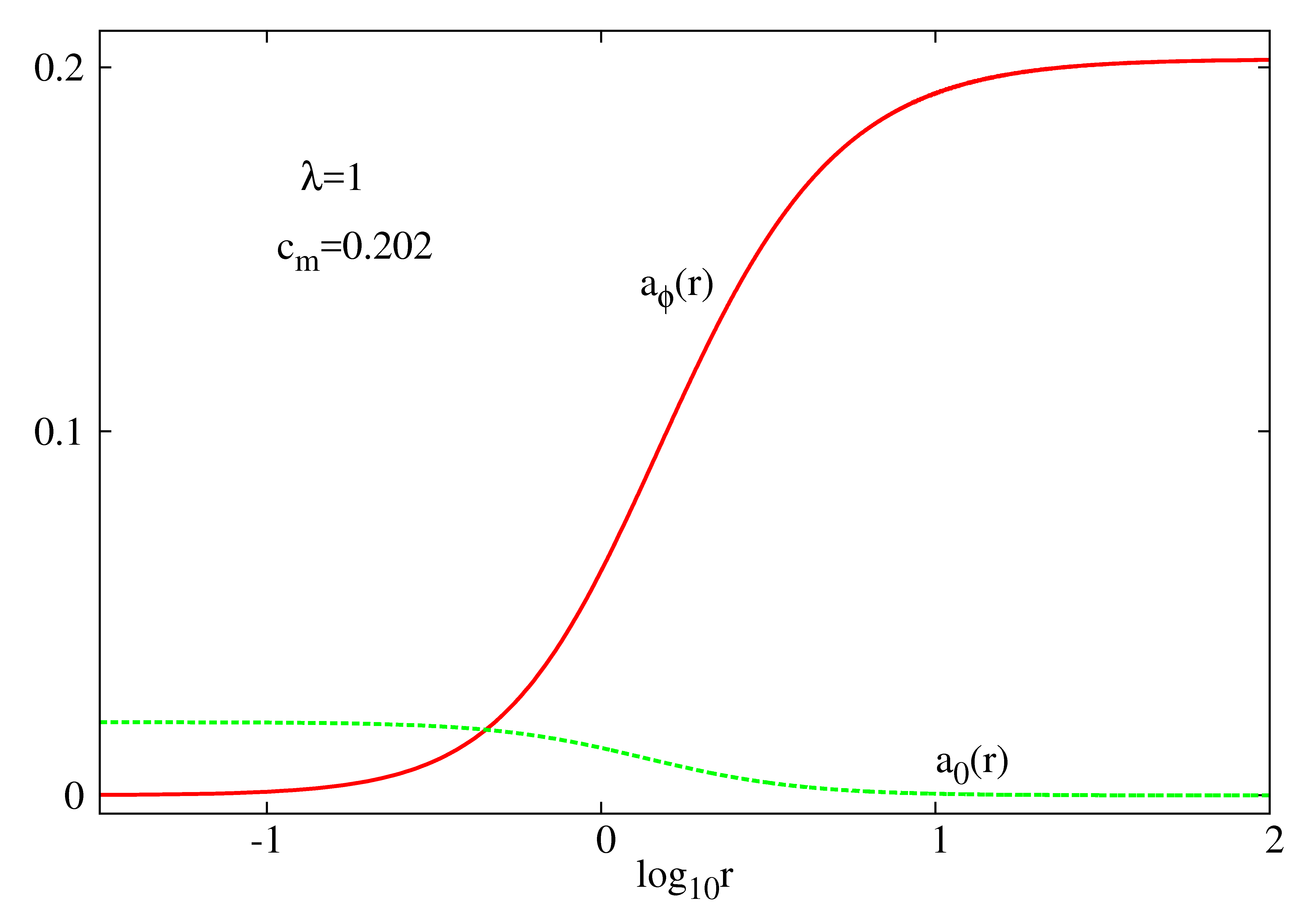
Figure 1: The profile of a typical solution of the Maxwell–Chern-Simons equations in a fixed AdS background.

The gauge field Ansatz contains an electric potential, $a_{0}$, and a magnetic one, $a_{\varphi}$ [3]

$$A=a_{0}(r)dt+a_{\varphi}(r)\frac{1}{2}\sigma_{3},$$ (6)

which results in the field strength tensor

$$F=a_{0}^{\prime}(r)dr\wedge dt+a_{\varphi}^{\prime}(r)\frac{1}{2}dr\wedge\sigma_{3}+\frac{1}{2}a_{\varphi}(r)\sigma_{2}\wedge\sigma_{1}~{}.$$ (7)

Then one writes the following MCS equations

$$\left(rN^{\prime}a_{\varphi}^{\prime}\right)^{\prime}=\left(1+\frac{8}{3}\frac{\lambda^{2}}{r^{2}}a_{\varphi}^{2}\right)\frac{4}{r}a_{\varphi},~{}~{}a_{0}^{\prime}=-\frac{4\lambda a_{\varphi}^{3}}{\sqrt{3}r^{3}}~{}.$$ (8)

For $\lambda=0$ ($i.e.$ a pure Maxwell field in AdS spacetime) the electric potential can be set to zero and one finds the following exact solution

$$a_{\varphi}(r)=c_{m}\left(1-\frac{L^{2}}{r^{2}}\log(1+\frac{r^{2}}{L^{2}})\right),$$ (9)

with $c_{m}$ an arbitrary (nonzero) constant. Unfortunately, the Eqs. (8) cannot be solved in closed form for $\lambda\neq 0$. However, such a solution exists; its small$-r$ expansion reads (with $u,v_{0},c_{m}$ and $\hat{\mu}$ nonzero constants):

$$a_{\varphi}(r)=ur^{2}+(-\frac{2}{3}\frac{u}{L^{2}}+\frac{8u^{3}\lambda^{2}}{9})r^{4}+\dots,~{}~{}a_{0}(r)=v_{0}-\frac{2u\lambda}{\sqrt{3}}r^{2}+\dots,$$ (10)

while its form for $r\to\infty$ is

$$a_{\varphi}(r)=c_{m}+\big{(}\hat{\mu}+2c_{m}L^{2}\log(\frac{L}{r})\big{)}\frac{1}{r^{2}}+\dots,~{}~{}a_{0}(r)=-\frac{2c_{m}^{2}\lambda}{\sqrt{3}}\frac{1}{r^{2}}+\dots.$$ (11)

This implies the existence of a nonvanishing asymptotic magnetic field, $F_{\theta\phi}\to-\frac{1}{2}c_{m}\sin\theta$, such that the parameter $c_{m}$ can be identified with the magnetic flux at infinity through the base space $S^{2}$ of the $S^{1}$ fibration,

$$\Phi_{m}=\frac{1}{4\pi}\int_{S^{2}_{\infty}}F=-\frac{1}{2}c_{m}.$$ (12)

The smooth profiles connecting the asymptotics (10) , (11) are constructed numerically, a typical example being shown in Figure 1.

Also, one can show that both $a_{\varphi}(r)$ and $a_{0}(r)$ are nodeless functions. Other properties of the MCS solutions are similar to those of their gravitating generalizations discussed in Section 3. Moreover, rather similar configurations are found when considering instead a Schwarzschild-AdS BH background.

2.3 The backreacting case

When taking into account the backreaction on the geometry, the solutions above should result in EMCS solitons and BHs. Unfortunately, it seems that no analytical techniques can be used to construct these solutions in closed form. As such, in this work we approach this problem by solving the EMCS equations numerically, subject to a set of boundary conditions compatible with an approximate expansion at the boundaries of the domain of integration.

The corresponding metric Ansatz is found by supplementing (5) with four undetermined functions which take into account the deformation of the AdS background and factorize the angular dependence allowing for configurations with two equal angular momenta

$$ds^{2}=-f(r)N(r)dt^{2}+\frac{1}{f(r)}\left[\frac{m(r)}{N(r)}dr^{2}+\frac{1}{4}r^{2}\left(m(r)(\sigma_{1}^{2}+\sigma_{2}^{2})+n(r)\big{(}\sigma_{3}-\frac{2\omega(r)}{r}dt\big{)}^{2}\right)\right],$$ (13)

while the gauge field Ansatz is still given by (6). This framework can be proven to be consistent, and, as a result, the EMCS equations reduce to a set of six second order ordinary differential equations plus a first order constraint equation, whose expression can be found in Ref. [14]. Also, these equations possess two first integrals

$$a_{0}^{\prime}+\frac{\omega}{r}a_{\varphi}^{\prime}-\frac{4\lambda}{\sqrt{3}}\frac{f^{3/2}a_{\varphi}^{2}}{r^{3}\sqrt{mn}}={\frac{2\,{f}^{3/2}}{\pi\sqrt{mn}{r}^{3}}}c_{1},~{}~{}~{}~{}~{}\frac{16\lambda}{3\sqrt{3}}a_{\varphi}^{3}-{\frac{{n}^{3/2}\sqrt{m}{r}^{3}}{{f}^{5/2}}}(r\omega^{\prime}-\omega)=c_{2}-{\frac{8\,c_{1}}{\pi}}\,a_{\varphi},$$ (14)

where $c_{1}$ and $c_{2}$ are two constants.

2.4 The asymptotics

In deriving the far field expression of the solutions, we impose that, asymptotically, $i)$ the geometry becomes AdS in a static frame, $ii)$ the electric potential vanishes, $a_{0}\to 0$; and, as a new feature as compared to the CLP case, $iii)$ the magnetic potential approaches a constant nonzero value, $a_{\varphi}\to c_{m}$. Then a far-field expression of a solution compatible with these assumptions can be constructed in a systematic way. The first few terms in this expansion read

$$f(r)=1+\left(\hat{\alpha}+\frac{12}{5}c_{m}^{2}L^{2}\log(\frac{L}{r})\right)\frac{1}{r^{4}}+\dots,~{}\omega(r)=\frac{\hat{J}}{r^{3}}-\frac{4q}{3}\left(\hat{\mu}-\frac{1}{3}c_{m}L^{2}(1-6\log(\frac{L}{r}))\right)\frac{1}{r^{5}}+\dots,$$

$$m(r)=1+\left(\hat{\beta}+\frac{4}{5}c_{m}^{2}L^{2}\log(\frac{L}{r})\right)\frac{1}{r^{4}}+\dots,~{}n(r)=1+\left(3(\hat{\alpha}-\hat{\beta})+\frac{4}{15}c_{m}^{2}L^{2}+\frac{24}{5}c_{m}^{2}L^{2}\log(\frac{L}{r})\right)\frac{1}{r^{4}}+\dots,~{}~{}{~{}~{}~{}}$$ (15)

$$a_{\varphi}(r)=c_{m}+\left(\hat{\mu}+2c_{m}L^{2}\log(\frac{L}{r})\right)\frac{1}{r^{2}}+\dots,~{}a_{0}(r)=-\frac{q}{r^{2}}+\frac{c_{m}\lambda}{\sqrt{3}}\left(2\hat{\mu}+c_{m}L^{2}\left(-1+4\log(\frac{L}{r})\right)\right)\frac{1}{r^{4}}+\dots,$$

with $\{\hat{\alpha},\hat{\beta},\hat{J};c_{m},\hat{\mu},q\}$ undetermined parameters.

Concerning the solitons, one can also construct a small-$r$ approximate form of the solutions as a power series in $r$, compatible with the assumption of regularity at $r=0$. The first terms in this expansion are

$$f(r)=f_{0}+\left(\frac{m_{0}-f_{0}}{L^{2}}+\frac{4u^{2}f_{0}^{2}}{3m_{0}}\right)r^{2}+\dots,~{}~{}m(r)=m_{0}+m_{2}r^{2}+\dots,~{}~{}\omega(r)=w_{1}r-\frac{8u^{3}f_{0}^{5/2}\lambda}{3\sqrt{3}m_{0}^{2}}r^{2}+\dots,$$

$$n(r)=m_{0}+\left(\frac{3m_{0}(m_{0}-f_{0})}{f_{0}L^{2}}-m_{2}+\frac{4u^{2}f_{0}}{3}\right)r^{2}+\dots,~{}~{}a_{0}(r)=v_{0}-\left(\frac{2u^{2}f_{0}^{3/2}\lambda}{\sqrt{3}m_{0}}+uw_{1}\right)r^{2}+\dots,$$ (16)

$$a_{\varphi}(r)=ur^{2}+\frac{u}{9f_{0}L^{2}m_{0}}\bigg{(}4u^{2}f_{0}^{2}L^{2}(1+2\lambda^{2})+3(4m_{0}^{2}-3f_{0}(2m_{0}+L^{2}M_{2}))\bigg{)}r^{4}+\dots,$$

with the free parameters $\{f_{0},m_{0},m_{2},w_{1};u,v_{0}\}.$

However, when gravitating solitons exist in a given model, normally one can also construct bound states of such solitons with an event horizon [17], [18]. These BHs have a horizon which is a squashed $S^{3}$ sphere and resides at a constant value of the quasi-isotropic radial coordinate $r=r_{H}>0$. The non-extremal solutions have the following expansion valid as $r\to r_{H}$

$$f(r)=f_{2}(r-r_{H})^{2}+O\left(r-r_{H}\right)^{3},~{}~{}m(r)=m_{2}(r-r_{H})^{2}+O\left(r-r_{H}\right)^{3},$$

$$n(r)=n_{2}(r-r_{H})^{2}+O\left(r-r_{H}\right)^{3},~{}~{}\omega(r)=\omega_{0}+O\left(r-r_{H}\right),$$ (17)

$$a_{0}(r)=a_{0}^{(0)}+O\left(r-r_{H}\right)^{2},~{}~{}a_{\varphi}(r)=a_{\varphi}^{(0)}+O\left(r-r_{H}\right)^{2},$$

with $\{f_{2},m_{2},n_{2},\omega_{0};a_{0}^{(0)},a_{\varphi}^{(0)}\}$ undetermined parameters. Also, note that the behavior of solutions inside the horizon ($r<r_{H}$) is not discussed in this work.

2.5 Physical parameters

In the next Section we give numerical evidence for the existence of smooth EMCS solutions interpolating between the asymptotics above. Most of the physical properties can be read off from the asymptotic data near the horizon/origin and at infinity.

The mass $M$ and angular momentum $J$ of these solutions is computed by using the quasilocal formalism [19], with a boundary stress tensor ${\rm T}_{ab}=\frac{2}{\sqrt{-h}}\frac{\delta I}{\delta h^{ab}}$. Then $M$ and $J$ are the conserved charges associated with Killing symmetries $\partial_{t}$, $\partial_{\psi}$ of the induced boundary metric $h$, found for a large constant value of $r$. This results in

$$M=-\frac{\pi}{8}\frac{(3\hat{\alpha}+\hat{\beta})}{L^{2}}+\frac{c_{m}^{2}\pi}{30}+\frac{3\pi}{32}L^{2},~{}~{}~{}~{}J=\frac{\pi}{4}\hat{J}.$$ (18)

The electric charge $Q$, as computed from the usual definition, is

$$Q=-\frac{1}{2}\int_{S_{\infty}^{3}}\tilde{F}=\pi q~{},$$ (19)

with ${\tilde{F}}_{\mu_{1}\mu_{2}\mu_{3}}\equiv\epsilon_{\mu_{1}\mu_{2}\mu_{3}\rho\sigma}F^{\rho\sigma}$. However, this quantity is not related to any conservation law if $c_{m}\neq 0$. A more appropriate definition is now the Page charge [20], [21],

$$Q^{(P)}=-\frac{1}{2}\int_{S_{\infty}^{3}}\left(\tilde{F}+\frac{\lambda}{\sqrt{3}}A\wedge F\right)=Q-\frac{2\pi}{\sqrt{3}}\lambda c_{m}^{2}\equiv c_{1}~{},$$ (20)

being related to the total derivative structure of the Maxwell-Chern-Simons equations (with $c_{1}$ the integration parameter we introduced in the first integral (14)).

Another physically relevant parameter one can define is the R-charge, associated with the conservation of the R-current of the dual theory at the AdS boundary [22]:

$$Q^{(R)}=-\frac{1}{2}\int_{S_{\infty}^{3}}\left(\tilde{F}+\frac{2\lambda}{3\sqrt{3}}A\wedge F\right)=Q-\frac{4\pi}{3\sqrt{3}}\lambda c_{m}^{2}~{}.$$ (21)

Note that these three charges coincide in the absence of a boundary magnetic field, $c_{m}=0$. Also, the first integral (14) implies that $\frac{1}{2}c_{m}Q^{(R)}+J=-\frac{\pi}{16}c_{2}$.

In the above relations, $\alpha$, $\beta$, $\hat{J}$ and $q$ are parameters which enter the far field expansion (15). Also, we remark that the interpretation proposed for $c_{m}$ in the probe limit, as a magnetic flux at infinity, still holds in the backreacting case.

Turning now to BH quantities defined in terms of the horizon boundary data in (16), we note that the solutions’ horizon angular velocity is

$$\Omega_{H}=\frac{\omega_{0}}{r_{H}},$$ (22)

while the area of the horizon $A_{H}$ and the Hawking temperature $T_{H}$ of the solutions are given by

$$A_{H}=2\pi^{2}r_{H}^{3}\frac{m_{2}}{f_{2}}\sqrt{\frac{n_{2}}{f_{2}}},~{}~{}~{}~{}T_{H}=\frac{1}{2\pi}\left(1+\frac{r_{H}^{2}}{L^{2}}\right)\frac{f_{2}}{\sqrt{m_{2}}}~{}.$$ (23)

The horizon electrostatic potential $\Phi_{H}$ as measured in a co-rotating frame on the horizon is

$$\Phi_{H}=a_{0}^{(0)}+\Omega_{H}a_{\varphi}^{(0)}.$$ (24)

Also, to have a measure of the squashing of the horizon, we introduce the deformation parameter

$$\varepsilon=\frac{n(r)}{m(r)}\bigg{|}_{r=r_{H}}=\frac{n_{2}}{m_{2}},$$ (25)

which gives the ratio of the $S^{1}$ and the round $S^{2}$ parts of the (squashed $S^{3}$) horizon metric, respectively.

Finally, let us remark that all configurations reported in this work have $f,m,n$ strictly positive functions for $r>r_{H}$ (or $r\geq 0$ for solitons). As such, $t$ is a global time coordinate and the metric is free of causal pathologies [23]. We have also monitored the Ricci and the Kretschmann scalars of the solutions and did not find any indication for a singular behavior.

3 The solutions

3.1 Solitons

The numerical results indicate the existence of a family of everywhere regular solutions with finite mass, charge and angular momentum. Such configurations can be viewed as deformations of the (globally) AdS background, corresponding to charged, spinning EMCS solitons. They possess no horizon, while the size of both parts of the $S^{3}$-sector of the metric shrinks to zero as $r\to 0$. The profile of a typical solution is exhibited in Figure 2 (left).

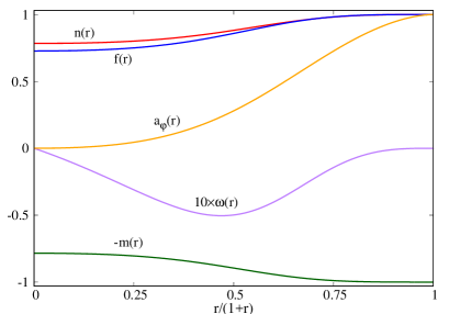
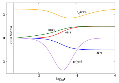
Figure 2: The profiles of a typical soliton with $c_{m}=1$, $L=1$ (left) and a typical black hole with $r_{H}=2$, $J=0$, $Q=10$, $c_{m}=10$ and $L=15$ (right).

The solitons have rather special properties. The only input parameter here is the constant $c_{m}$ which fixes the magnitude at infinity of the magnetic potential. For any $\lambda\neq 0$, the electric charge and angular momentum are given by

$$J=-\frac{\lambda\pi}{3\sqrt{3}}c_{m}^{3},~{}~{}~{}~{}Q=3Q^{(R)}=\frac{2\lambda\pi}{\sqrt{3}}c_{m}^{2}~{},$$ (26)

such that the following universal relation is satisfied

$$J=\Phi_{m}Q^{(R)},$$ (27)

with $\Phi_{m}$ computed from (12).

The $M(c_{m})$ dependence can be found only numerically, being displayed in Figure 3. A good fit up to a relatively high value $c_{m}\sim 4$ reads

$$\frac{M}{L^{2}}=\frac{3\pi}{32}+a_{2}\frac{c_{m}^{2}}{L^{2}}+a_{4}\frac{c_{m}^{4}}{L^{4}}+a_{6}\frac{c_{m}^{6}}{L^{6}}~{},$$ (28)

with $a_{2}=-1.52$, $a_{4}=0.175$, $a_{6}=-0.0025$, and variance of residuals of $3\times 10^{-4}$. Note that no upper bound on $|c_{m}|$ seems to exist; however, the numerics becomes difficult for large values of it. Also, similar to the probe limit, we could not find excited solutions (which would possess a magnetic potential with nodes [14]); this holds also in the BH case. However, we conjecture the existence of such solutions for large enough values of the CS coupling constant $\lambda$.

3.2 Black holes

As expected, these solutions possess BH generalizations. They can be constructed starting with $any$ CLP solution and slowly increasing the value of the parameter $c_{m}$. The profile of a typical BH is shown in Figure 2 (right).

Finding the domain of existence of these BHs together with their general properties is a considerable task which is not aimed at in this paper. Instead, we analyze several particular classes of solutions, looking for special properties.

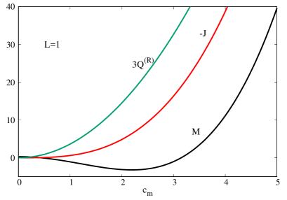
Figure 3: The mass, angular momentum and electric charge of gravitating spinning solitons are shown as a function of the magnetic parameter $c_{m}$.

In Figure 4 we display the results for configurations with fixed values of both $Q^{(R)}$ and $J$ and several values of $c_{m}$. The first feature we notice is that $c_{m}\neq 0$ leads to some differences for small values of $T_{H}$ only, while the solutions with large temperatures are essentially CLP BHs. Also, as expected, the qualitative behavior of solutions with small $|c_{m}|$ resembles that of the unmagnetized case. However, this changes for large enough values of $c_{m}$ and one finds $e.g.$ a monotonic behavior of mass and horizon area as a function of temperature. In particular, this means that for large values of $|c_{m}|$, the BHs become thermodynamically stable for the full range of $T_{H}$, with the existence of one branch of solutions only. Also, the sign of $c_{m}$ is relevant for small values of $|c_{m}|$, only.

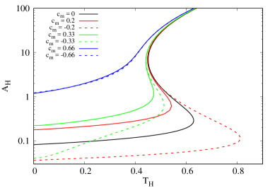
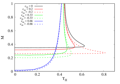
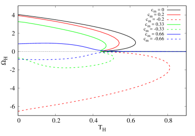
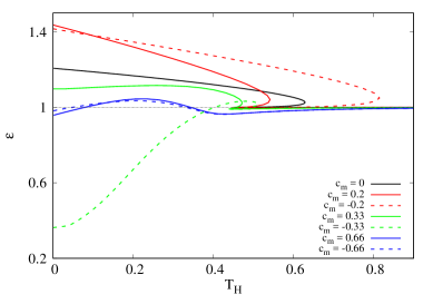
Figure 4: Area $A_{H}$, mass $M$, angular velocity $\Omega_{H}$ and horizon deformation $\varepsilon$, as a function of the horizon temperature $T_{H}$ and for several values of the magnetic flux on the boundary. These solutions have AdS length $L=1$, angular momentum $J=0.003$, and the R-charge $Q^{(R)}=0.044$.

More unusual features occur as well. For example, in contrast with the CLP case, one finds BHs which have $J=0$ but still rotate in the bulk. Some results in this case are shown in Figure 5 for solutions with a fixed value of the electric charge $Q^{(R)}=-0.044$. These 3D plots exhibit the temperature as a function of $c_{m}$ and horizon area, mass and horizon angular velocity, respectively. The $(T_{H};c_{m},R(r_{H}))$-diagram is also included there (with $R(r_{H})$ the Ricci scalar evaluated at the horizon), to show that these BHs possess a regular horizon.

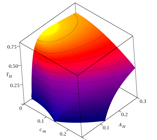
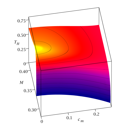
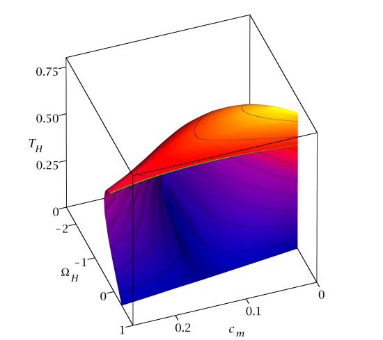
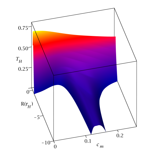
Figure 5: The area $A_{H}$, mass $M$, angular velocity $\Omega_{H}$ and Ricci scalar $R(r_{H})$ of magnetized black holes are shown as a function of $(T_{H},c_{m})$. These solutions have $L=1$, a fixed electric charge $Q^{(R)}=-0.044$ and a vanishing angular momentum, $J=0$.

4 Further remarks

The main purpose of this paper was to report a generalization of the known Cvetič, Lü and Pope (CLP) BH solutions [3] of the $D=5$ minimal gauged supergravity, which contains an extra-parameter in addition to mass, electric charge and angular momentum. This extra-parameter can be identified with the magnitude of the magnetic potential at infinity. As such, the solutions here can be viewed as the simplest AdS₅ generalizations of the $D=4$ Einstein-Maxwell solitons and BHs recently reported in the literature [6]-[9]. Thus one can predict the existence of a variety of other $D=5$ solutions with the U(1) potentials satisfying non-standard far field boundary conditions.

The most interesting new feature as compared to the CLP case is perhaps the existence of a one parameter family of globally regular, smooth solitonic configurations. Different from the previously known EMCS solitons with $c_{m}=0$ which are supported by the nontrivial topology of spacetime [23], the solutions here can be considered as deformations of the globally AdS background and require a non-vanishing magnetic field on the boundary. We also remark that both the BHs and the solitons can be uplifted to type IIB or to eleven-dimensional supergravity by using the standard results in the literature (see $e.g.$ [24], [25], [26]).

The study of these magnetized solutions in an AdS/CFT context is an interesting open question. For example, the background metric upon which the dual field theory resides is a $D=4$ static Einstein universe with a line element $ds^{2}=\gamma_{ab}dx^{a}dx^{b}=-dt^{2}+\frac{1}{4}L^{2}(\sigma_{1}^{2}+\sigma_{2}^{2}+\sigma_{3}^{2}).$ However, different from the solution in [3], in this case the theory is formulated in a background $U(1)$ gauge field, with ${\rm F}_{(0)}=\frac{1}{2}c_{m}\sigma_{2}\wedge\sigma_{1}$. The expectation value of the stress tensor of the dual theory can be computed by using the AdS/CFT “dictionary”, with $\sqrt{-\gamma}\gamma^{ab}<\tau_{bc}>=$$\lim_{r\to\infty}\sqrt{-h}h^{ab}{\rm T}_{bc}$.

The nonvanishing components of $<\tau_{ab}>$ are

$$<\tau_{\theta}^{\theta}>=<\tau_{\phi}^{\phi}>=\frac{1}{8\pi L}\left(\frac{1}{8}-\frac{5(\hat{\alpha}-\hat{\beta})}{2L^{4}}-\frac{32c_{m}^{2}}{15L^{2}}\right),~{}<\tau_{\psi}^{\psi}>=\frac{1}{8\pi L}\left(\frac{1}{8}-\frac{7\hat{\alpha}-11\hat{\beta}}{2L^{4}}+\frac{2c_{m}^{2}}{5L^{2}}\right),~{}~{}$$

$$<\tau_{\phi}^{\psi}>=\cos\theta\big{(}<\tau_{\psi}^{\psi}>-<\tau_{\phi}^{\phi}>\big{)},~{}<\tau_{\psi}^{t}>=\frac{1}{\cos\theta}<\tau_{\phi}^{t}>=-\frac{1}{4}L^{2}<\tau_{t}^{\psi}>=\frac{\hat{J}}{8\pi L^{3}},$$

$$<\tau_{t}^{t}>=\frac{1}{8\pi L}\left(-\frac{3}{8}+\frac{3\hat{\alpha}+\hat{\beta}}{2L^{4}}-\frac{2c_{m}^{2}}{15L^{2}}\right).$$

The trace of this tensor is nonzero, with

$$<\tau_{a}^{a}>=-\frac{c_{m}^{2}}{2\pi L^{3}}=-\frac{L}{64\pi}{\rm F}_{(0)}^{2},$$ (29)

resulting from the coupling of the dual theory to a background gauge field [28]. An interesting question here concerns the possible existence, within the proposed framework, of configurations possessing a Killing spinor. However, the results in [29] show that this is not the case: a supersymmetric solution with a nonzero boundary magnetic field is not compatible with the far field asymptotics (15), requiring a $squashed$ $S^{3}$ sphere at infinity.

As avenues for future research, we remark that the framework and the preliminary results proposed in this work may provide a fertile ground for the further study of charged rotating configurations in the $D=5$ gauged supergravity model. For example, it would be interesting to study in a systematic way their domain of existence, together with the extremal limit. Moreover, one expects some of the solutions’ properties to be generic when adding scalars or taking unequal spins. We hope to return elsewhere with a discussion of some of these aspects.

Acknowledgement
We gratefully acknowledge support by the DFG Research Training Group 1620 “Models of Gravity” and by the Spanish Ministerio de Ciencia e Innovación, research project FIS2011-28013. E. R. acknowledges funding from the FCT-IF programme. This work was also partially supported by the H2020-MSCA-RISE-2015 Grant No. StronGrHEP-690904, and by the CIDMA project UID/MAT/04106/2013. J.L.B.S. and J.K. gratefully acknowledge support by the grant FP7, Marie Curie Actions, People, International Research Staff Exchange Scheme (IRSES-606096). F. N.-L. acknowledges funding from Complutense University under Project No. PR26/16-20312.

References

- [1] J. M. Maldacena, Int. J. Theor. Phys. 38 (1999) 1113 [Adv. Theor. Math. Phys. 2 (1998) 231] [hep-th/9711200].
- [2] E. Witten, Adv. Theor. Math. Phys. 2 (1998) 253 [hep-th/9802150].
- [3] M. Cvetic, H. Lü and C. N. Pope, Phys. Lett. B 598 (2004) 273 [hep-th/0406196].
- [4] Z. W. Chong, M. Cvetic, H. Lü and C. N. Pope, Phys. Rev. Lett. 95 (2005) 161301 [arXiv:hep-th/0506029];
- [5] J. B. Gutowski and H. S. Reall, JHEP 0402 (2004) 006 [hep-th/0401042].
- [6] C. Herdeiro and E. Radu, Phys. Lett. B 749 (2015) 393 [arXiv:1507.04370 [gr-qc]].
- [7] M. S. Costa, L. Greenspan, M. Oliveira, J. Penedones and J. E. Santos, Class. Quant. Grav. 33 (2016), 115011 [arXiv:1511.08505 [hep-th]].
- [8] C. Herdeiro and E. Radu, Phys. Lett. B 757 (2016) 268 [arXiv:1602.06990 [gr-qc]].
- [9] C. A. R. Herdeiro and E. Radu, Phys. Rev. Lett. 117, 221102 (2016) [arXiv:1606.02302 [gr-qc]].
- [10] J. L. Blázquez-Salcedo, J. Kunz, F. Navarro-Lérida and E. Radu, Entropy 18, 438 (2016) [arXiv:1612.03747 [gr-qc]].
- [11] P. Chrusciel and E. Delay, Lett. Math. Phys. (2017) arXiv:1612.00281 [math.DG].
- [12] P. T. Chruściel, E. Delay and P. Klinger, arXiv:1701.03718 [gr-qc].
- [13] J. L. Blázquez-Salcedo, J. Kunz, F. Navarro-Lérida and E. Radu, Phys. Rev. D 92 (2015), 044025 [arXiv:1506.07802 [gr-qc]].
- [14] J. L. Blázquez-Salcedo, J. Kunz, F. Navarro-Lérida and E. Radu, Phys. Rev. D 95 (2017), 064018 [arXiv:1610.05282 [gr-qc]].
-
[15]
U. Ascher, J. Christiansen, R. D. Russell,
Math. Comput. 33 (1979) 659;
U. Ascher, J. Christiansen, R. D. Russell, ACM Trans. 7 (1981) 209. -
[16]
P. G. Nedkova and S. S. Yazadjiev,
Phys. Rev. D 85 (2012) 064021
[arXiv:1112.3326 [hep-th]];
P. G. Nedkova and S. S. Yazadjiev, Eur. Phys. J. C 73 (2013), 2377 [arXiv:1211.5249 [hep-th]]. - [17] D. Kastor and J. H. Traschen, Phys. Rev. D 46 (1992) 5399 [hep-th/9207070].
- [18] M. S. Volkov and D. V. Gal’tsov, Phys. Rept. 319 (1999) 1 [hep-th/9810070].
- [19] V. Balasubramanian and P. Kraus, Commun. Math. Phys. 208 (1999) 413 [hep-th/9902121].
- [20] D. N. Page, Phys. Rev. D 28 (1983) 2976.
- [21] D. Marolf, ”Chern-Simons terms and the three notions of charge”, hep-th/0006117.
- [22] O. Aharony, S. S. Gubser, J. M. Maldacena, H. Ooguri and Y. Oz, Phys. Rept. 323 (2000) 183 [hep-th/9905111].
- [23] M. Cvetic, G. W. Gibbons, H. Lü and C. N. Pope, ”Rotating black holes in gauged supergravities: Thermodynamics, supersymmetric limits, topological solitons and time machines”, hep-th/0504080.
- [24] A. Chamblin, R. Emparan, C. V. Johnson and R. C. Myers, Phys. Rev. D 60 (1999) 064018 [hep-th/9902170].
- [25] J. P. Gauntlett, D. Martelli, J. Sparks and D. Waldram, Class. Quant. Grav. 21 (2004) 4335 [hep-th/0402153].
- [26] J. P. Gauntlett and O. Varela, Phys. Rev. D 76 (2007) 126007 [arXiv:0707.2315 [hep-th]].
-
[27]
E. D’Hoker and P. Kraus,
JHEP 1003 (2010) 095
[arXiv:0911.4518 [hep-th]];
E. D’Hoker and P. Kraus, JHEP 0910 (2009) 088 [arXiv:0908.3875 [hep-th]]. - [28] M. Taylor, ”More on counterterms in the gravitational action and anomalies”, hep-th/0002125.
- [29] D. Cassani and D. Martelli, JHEP 1408 (2014) 044 [arXiv:1402.2278 [hep-th]].