A Java library to perform S-expansions
of Lie algebras

Abstract

The contraction method is a procedure that allows to establish non-trivial relations between Lie algebras and has had succesful applications in both mathematics and theoretical physics. This work deals with generalizations of the contraction procedure with a main focus in the so called S-expansion method as it includes most of the other generalized contractions. Basically, the S-exansion combines a Lie algebra $\mathcal{G}$ with a finite abelian semigroup $S$ in order to define new S-expanded algebras. After giving a description of the main ingredients used in this paper, we present a Java library that automatizes the S-expansion procedure. With this computational tool we are able to represent Lie algebras and semigroups, so we can perform S-expansions of Lie algebras using arbitrary semigroups. We explain how the library methods has been constructed and how they work; then we give a set of example programs aimed to solve different problems. They are presented so that any user can easily modify them to perform his own calculations, without being necessarily an expert in Java. Finally, some comments about further developements and possible new applications are made.

1 Introduction

The theory of Lie groups and algebras plays an important role in physics, as it allows to describe the continues symmetries of a given physical system. Due to the well-known relation between symmetries and conservation laws, via the Noether theorem, the Lie theory represents an essential ingredient in the construction of quantum field theories, particularly in the Standard Model of particles, as well as in general relativity and its generalizations. Since the second half of the last century, the study of non-trivial relations between Lie algebras and groups appears also as a problem of great interest in both mathematics and modern theoretical physics. Examples of these procedures are known as contractions [1, 2, 3] and deformations [4, 5, 6] of Lie algebras, both sharing the property of preserving the dimension of the algebras involved in the process.

The idea that lead to the concept of contractions was first introduced in Ref. [1] and consists in the observation that if two physical theories are related by means of a limit process, then the corresponding symmetry groups under which those theories are invariant should be related through a limit process too. For example, the Newtonian mechanics can be obtained from special relativity by taking $c\rightarrow\infty$ (where $c$ is the speed of light) and thus, the non-relativistic limit that brings the Poincaré algebra to the Galilean algebra is a good example of what is called a contraction process. On the other part, a deformation can be regarded as the inverse of a contraction, which means that in the previous example the Poincaré algebra is a deformation of the Galilean algebra. However, in the present article we will not work with deformations, but rather with generalizations of the contraction method.

The contractions were formally introduced in Ref. [2] in a way that nowdays it is known as Inönü-Wigner (IW) contraction. The contraction $\mathcal{G}_{c}$ of an algebra $\mathcal{G}$ is made with respect to a subalgebra $\mathcal{L}_{0}$ of $\mathcal{G}$. The procedure bassically consists in rescaling the generators of $\mathcal{G}/\mathcal{L}_{0}$ by a parameter $\lambda$ and then to perform a singular limit for that parameter. As a result, the generators of $\mathcal{G}/\mathcal{L}_{0}$ becomes abelian and the subalgebra acts on them. Further details and explicit examples, including the mentioned relation between Galileo and Poincaré algebras, can be found in Refs. [7, 8]. Remarkably, if the original algebra have a more general subspace structure, it is possible to perform more general contractions which are known as Weimar-Woods (WW) contractions [9].

Recently, an interesting generalization has been parallelly introduced in the context of string theory [10] and supergravity [11, 12, 13]. This procedure, known as expansion method, is not only able to reproduce the WW contractions when the dimension is preserved in the process, but also may lead to expanded algebras whose dimension is higher than the original one (a result that cannot be obtained by any contraction process). Another distinguishing feature is that the algebra is described in its dual formalism, i.e., in terms of the Maurer-Cartan (MC) forms on the manifold of its associated Lie group (a good introduction to the dual formulation of Lie algebras can be found in Chapter 5.6 of [14]). Instead of rescaling the generators by a real parameter $\lambda$, as it is usually made in the contractions methods, the rescaling is performed on some of the group coordinates. As a consequence, the MC forms can be expanded as power series in $\lambda$ that under certain conditions can be trucated in such a way that assures the closure of a new bigger algebra.

In this work we deal with an even more general procedure called S-expansion [15] that not only reproduces the results of expansion method described before (which means in turn that also reproduces all WW contractions), but also allows to establish relations between Lie algebras that cannot be obtained by the previous expansion procedure. Instead of performing a rescaling of some of the algebra generators or the group coordinates, it combines the structure constants of the algebra $\mathcal{G}$ with the inner multiplication law of an abelian semigroup $S$ in order to define the Lie bracket of a new S-expanded algebra. Under certain conditions, it is possible to extract smaller algebras which are called resonant subalgebras and reduced algebras. On that stage, the S-expansion is able to reproduce the results of the previous expansion method [10, 11], for a particular family of semigroups denoted by $S_{E}^{\left(N\right)}$.

An important advantage of the S-expansion method is related with the construction of invariant tensors (and their duals known as Casimir operators) whose full classification is known only for semisimple Lie algebras. The standard procedure to construct an invariant tensor of range $r$ is to use the symmetrized trace (or supertrace for superalgebras) for the product of $r$ generators in some matrix representation. The good feature of the S-expansion is that if we know the invariant tensors of a certain semisimple Lie algebra, then the mechanism gives the invariant tensors for the expanded algebras even if they are not semisimple (the same result was extended in Ref. [16] for the Casimir operators). Those invariant tensors of the S-expanded algebra are in general different from the symmetrized trace so it would be interesting to analyze if the S-expansion could help to solve the classification of invariant tensors for non-semisimple Lie algebras. Indeed, it has already been supposed in the early 60’s that solvable Lie algebras could be obtained as contractions of semisimple algebras of the same dimension [17, 18]. The incorrectness of that conjecture was shown in Ref. [19] and, recently, that problem has been revisited in terms of S-expansions [20]. However, to know whether S-expansions are able to fit the classification of non-semisimple Lie algebras and their invariant tensors, remains an open problem. Independently of the answer, what we do know is that the S-expansion gives invariant tensors that are in general different from the symmetrized trace and this fact has already been useful for the construction of Chern-Simons (CS) gauge theories of (super)gravity [21, 22] and their interrelations.

The dual formulation [23] in terms of MC forms has also been very useful, as it allows to perform the S-expansion procedure directly on the Lagrangian of a given gravity theory. This has been used in Refs. [24, 25, 26, 27, 28] to show that General Relativity (GR) in even and odd dimensions may emerge as a special limit of a Born Infeld [29] and CS Lagrangian respectively. Black hole and cosmological solutions has been studied for gravity theories based on expanded algebras Refs. [30, 31, 32, 33], as well as some aspects about their non relativistic limits [34]. In addition, the S-expansion has also been extended to other mathematical structures, like the case of higher order Lie algebras and infinite dimensional loop algebras [35, 36, 37].

At the begining, the applications considered only the specific family of semigroups that allows to reproduce the previous expansion method [10, 11]. These semigroups were denoted by $S_{E}^{(N)}$ and lead to the so called $\mathfrak{B}_{N}$ algebras [15]. The use of others abelian semigroups to perform S-expansions of Lie algebras was first considered in Ref. [38]. It was shown that some Bianchi algebras [39] can be obtained as S-expansions form the two dimensional isometries acting transitively in a two-dimensional space. The semigroups that allows to obtain those relations are not all belonging to the $S_{E}^{(N)}$ family and thus, it is clear that these results can only be obtained in the context of the S-expansion, i.e., they cannot be reached by using the previous expansion procedure [11]. This procedure was then used in Ref. [16] to show that the semisimple version of the so called Maxwell algebra (introduced in [40, 41, 42]) can be obtained as an expansion of the AdS algebra. Later, this result was generalized in Refs. [43, 44] to new families of semigroups generating algebras denoted by $\mathfrak{C}_{N}$ and $\mathfrak{D}_{N}$ which have been useful to construct new (super)gravity models [45, 46, 47, 48, 49, 50, 51, 52]. Other recent applications can also be found in [53, 54].

On the other hand, a general study of the properties $S$-expansion with arbitrary semigroups, in the context of the classification of Lie algebras, was performed in [55]. It was shown that under the S-expansions some properties of the original algebra are always preserved while others do not in general. The explicit examples that allowed to check the results in Refs. [38] and [55] were obtained with a set computing programs that, in this work, we have improved and further developed to give them in the form of a Java library [56] allowing to perform S-expansions with arbitrary finite abelian semigroups. We will present this library as a handbook with examples and all the necessary information to use its methods.

This work is organized as follows: In section 2 we introduce the basic ingredients we will use. First, we give a brief description of discrete semigroups and the $S$-expansion method. Then we give a brief review about the existing literature about the classification of non-isomorphic semigroups and finite semigroup computer programs. We conclude that section with a general description of the library and notation used. In sections 3 and 4 we describe the library, which consists of a set of classes containing different methods allowing us to perform S-expansions with any given finite abelian semigroup. The reader who is not an expert in Java language and/or probably is more interested in applying the computational tools presented in this paper, might skip Sections 3 and 4 and go directly to Section 5. There, we describe some of the 45 programs provided in [56] (see the list in Appendix A) as examples to use the library. With those instructions the user can easily create new programs to perform his own calculations just by changing the inputs and even without knowing about Java language. Finally, Section 6 contains some comments about possible new applications.

2 Preliminars

2.1 Discrete semigroups

We consider a set of $n$ elements $S=\{\lambda_{\alpha},\alpha=1,\cdots,n\}$. We say that $S$ is a semigroup if it is equipped with an associative product

$$\cdot:$$

 .

Notice that:

• It does not exist necessarily the identity element $e$ satisfying $\lambda_{\alpha}\cdot\,e=\lambda_{\alpha}\;\forall\alpha=1,\ldots,n$

• The elements $\lambda_{\alpha}$ do not need to have an inverse.

• If there exists an element $0_{S}$ such that $\lambda_{\alpha}\cdot 0_{S}=0_{S}\;\forall\alpha$ we will call it a zero element

• $n$ is the order of the semigroup

• If $\lambda_{\alpha}\cdot\lambda_{\beta}=\lambda_{\beta}\cdot\lambda_{\alpha}$, the discrete semigroup is said to be commutative or abelian

We can give the product by means of a multiplication table, a $n\times n$ matrix

$$A=\begin{pmatrix}a_{\alpha\beta}\end{pmatrix}\equiv\begin{pmatrix}\lambda_{\alpha}\cdot\lambda_{\beta}\end{pmatrix}\,,$$ (1)

with entries in $\lambda_{\alpha}$. Thus, a visual way to describe a semigroup is given by,

λ1⋮λαλκ​(α,β)⋮λn.fragments fragmentsλ1missing-subexpressionmissing-subexpressionmissing-subexpressionmissing-subexpressionmissing-subexpression⋮missing-subexpressionmissing-subexpressionmissing-subexpressionmissing-subexpressionmissing-subexpressionfragmentsλ𝛼missing-subexpressionmissing-subexpressionfragmentsλ𝜅𝛼𝛽missing-subexpressionmissing-subexpression⋮missing-subexpressionmissing-subexpressionmissing-subexpressionmissing-subexpressionmissing-subexpressionfragmentsλ𝑛missing-subexpressionmissing-subexpressionmissing-subexpressionmissing-subexpressionmissing-subexpression\begin{tabular}[c]{c|ccccc}&$\lambda_{1}$&$\cdots$&$\lambda_{\beta}$&$\cdots$&$\lambda_{n}$\\ \hline\cr$\lambda_{1}$&&&&&\\ $\vdots$&&&&&\\ $\lambda_{\alpha}$&&&$\lambda_{\kappa\left(\alpha,\beta\right)}$&&\\ $\vdots$&&&&&\\ $\lambda_{n}$&&&&&\end{tabular}\,.

λ1⋯λβ⋯λnλ1⋯λβ⋯λn (2)

For instance, it allows us to check easily if a semigroup is commutative, because in that case its multiplication table is symmetric.

An informal way (but useful for our purposes) of expressing the multiplication group law is by means of the quantities $K_{\alpha\beta}^{\kappa}$, called selectors, which are defined in the following way

$$K_{\alpha\beta}^{\kappa}=\begin{cases}1\;\hbox{if}\;\lambda_{\alpha}\cdot\lambda_{\beta}=\lambda_{\kappa}\,,\\ 0\;\hbox{if}\;\lambda_{\alpha}\cdot\lambda_{\beta}\neq\lambda_{\kappa}\,.\\ \end{cases}$$ (3)

Then, the semigroup law can be expressed as follows:

$$\lambda_{\alpha}\cdot\lambda_{\beta}=K_{\alpha\beta}^{\kappa}\lambda_{\kappa}\,.$$ (4)

As shown explicitly in Ref. [15], from the associativity and closure of the semigroup it follows that the selectors provide a matrix representation for $S$ and this fact that will be used in the next section to define the S-expansion method.

Isomorphisms of semigroups

Consider the semigroups given by the following multiplication tables,

λ1λ1λ1λ2λ1λ1, λ1λ2λ2λ2λ2λ2.fragments fragmentsλ1fragmentsλ1fragmentsλ1fragmentsλ2fragmentsλ1fragmentsλ1fragments fragmentsλ1fragmentsλ2fragmentsλ2fragmentsλ2fragmentsλ2fragmentsλ2\begin{tabular}[c]{c|cc}&$\lambda_{1}$&$\lambda_{2}$\\ \hline\cr$\lambda_{1}$&$\lambda_{1}$&$\lambda_{1}$\\ $\lambda_{2}$&$\lambda_{1}$&$\lambda_{1}$\end{tabular}\,,\ \ \begin{tabular}[c]{c|cc}&$\lambda_{1}$&$\lambda_{2}$\\ \hline\cr$\lambda_{1}$&$\lambda_{2}$&$\lambda_{2}$\\ $\lambda_{2}$&$\lambda_{2}$&$\lambda_{2}$\end{tabular}\,.

λ1λ2λ1λ2λ1λ2λ1λ2 (5)

These two semigroups have exactly the same structure if we rename $\lambda_{1}$ by $\lambda_{2}$ and viceversa. This is an example of an isomorphism of semigroups.

The group of isomorphisms between semigroups of order $n$ is isomorphic to the group of permutations of $n$ elements $\Sigma_{n}$. For simplicity, we choose to represent a permutation by

$$\left(\lambda_{\alpha_{1}}\,\lambda_{\alpha_{2}}\cdots\lambda_{\alpha_{n}}\right)$$ (6)

which means change $\lambda_{1}$ by $\lambda_{\alpha_{1}}$ , change $\lambda_{2}$ by $\lambda_{\alpha_{2}}$ , $\cdots$ , and finally change $\lambda_{n}$ by $\lambda_{\alpha_{n}}$. Then, isomorphisms between semigroups can be defined in terms of their multiplication tables. Let $A=\begin{pmatrix}a_{\alpha\beta}\end{pmatrix}$ and $B=\begin{pmatrix}b_{\alpha\beta}\end{pmatrix}$ be the multiplication tables of two semigroups of order $n$. According to the definitions given in Ref. [57], $A$ and $B$ describe two isomorphic semigroups if there exists a permutation $\sigma\in\Sigma_{n}$ such that

$$A\sigma=B\longleftrightarrow b_{\alpha\beta}=\sigma(a_{\sigma^{-1}(\alpha),\sigma^{-1}(\beta)})\,\,\,\,\forall\alpha,\,\beta=1,\ldots,n.$$ (7)

If, instead, we have

$$b_{\alpha\beta}=\sigma(a_{\sigma^{-1}(\beta),\sigma^{-1}(\alpha)})$$ (8)

we say that $A$ and $B$ are related by an anti-isomorphism.

2.2 $S$-Expansion of Lie algebras

Here we briefly describe the general abelian semigroup expansion procedure (S-expansion for short). We refer the interested reader to Refs.[15] for further details.

First, we need to consider a Lie algebra $\mathcal{G}$ with generators $\{X_{i}\}$ and Lie bracket

$$\left[X_{i},X_{j}\right]=C_{ij}^{\,\,\,\,k}X_{k}\,.$$ (9)

where $C_{ij}^{\,\,\,\,k}$ are the structure constants. Next, we need a finite abelian semigroup $S=\left\{\lambda_{\alpha}\right\}$, whose multiplication law is given in terms of the selectors $K_{\alpha\beta}^{\gamma}$ defined in Eqs. (3,4). According to Theorem 3.1 from ref.[15], the direct product

$$\mathcal{G}_{S}\text{\ }\mathcal{=}\text{\ }S\otimes\mathcal{G}$$ (10)

is also a Lie algebra, which is called expanded algebra. In the proof it can be seen that the commutativity property of the semigroup is crucial for the Jacobi identity to be satisfied in $\mathcal{G}_{S}$. The elements of this expanded algebra are denoted by

$$X_{\left(i,\alpha\right)}=\lambda_{\alpha}\otimes X_{i}\,,$$ (11)

where $\otimes$ is the Kronecker product of the matrix representations of the generators $X_{i}\in\mathcal{G}$ and the semigroup elements $\lambda_{a}\in S$. The Lie bracket in $\mathcal{G}_{S}$ is defined as

$$\left[T_{\left(i,\alpha\right)},T_{\left(j,\beta\right)}\right]=C_{\left(i,\alpha\right)\left(j,\beta\right)}^{\left(k,\gamma\right)}T_{\left(k,\gamma\right)}\equiv\lambda_{\alpha}\cdot\lambda_{\beta}\otimes\left[T_{i},T_{j}\right]$$ (12)

and therefore the structure constants of the expanded algebra $\mathcal{G}_{S}$ are fully determined by the selectors and the structure constants of the original Lie algebra $\mathcal{G}$, i.e.,

$$C_{\left(i,\alpha\right)\left(j,\beta\right)}^{\left(k,\gamma\right)}=K_{\alpha\beta}^{\gamma}C_{ij}^{k}\,.$$ (13)

There are different cases in which it is possible to systematically extract smaller algebras from $S\otimes\mathcal{G}$. One of them it occurs when the Lie algebra has a decomposition in a direct sum of vectorial subspaces $\mathcal{G}=\bigoplus_{p\in I}V_{p}$, where $I$ is a set of indices encoding the information of the internal subspace structure of the algebra through the mapping $i:I\otimes I\rightarrow 2^{I}$ and the relation

$$\left[V_{p},V_{q}\right]\subset{\displaystyle\bigoplus\limits_{r\in i\left(p,q\right)}}V_{r}\,.$$ (14)

If the semigroup $S$ has a decomposition in subsets $S_{p}$, $S=\bigcup_{p\in I}S_{p}$, satisfying the condition

$$S_{p}\cdot S_{q}\subset{\displaystyle\bigcap\limits_{r\in i\left(p,q\right)}}S_{r}\,,$$ (15)

which is said to be resonant with respect to the subspace structure (14) of the algebra, then the subset

$$\mathcal{G}_{S,R}=\bigoplus_{p\in I}S_{p}\otimes V_{p}$$ (16)

is a Lie algebra by itself, which is called resonant subalgebra of $\mathcal{G}_{S}$ (see Theorem 4.2 from ref. [15]).

Before explaining the next procedures to extract a smaller algebra from $\mathcal{G}_{S}$ we need to briefly explain what is called a reduction of an algebra. Supose that we have a Lie algebra with a subspace decomposition $\mathcal{G}=V_{0}\oplus V_{1}$. If the condition $\left[V_{0},V_{1}\right]\subset V_{1}$ is statisfied, then it is possible to show that the structure constants on $V_{0}$ satisfies the Jacobi identity by themselves (the proof can be found in Chapter 4.1.2 of Ref. [58]). The structure constants whose indices take values only on $V_{0}$ defines then a Lie algebra, which is called reduced algebra $\left|V_{0}\right|$. Notice that this definition does not require that $V_{0}$ is a subalgebra.

Now, the second case in which is possible to obtain a smaller algebra occurs when there is a zero element in the semigroup $S=\left\{\lambda_{\alpha},0_{S}\right\}$. In that case the commutation relations of $\mathcal{G}_{S}$ are given by,

$$\left[X_{\left(i,\alpha\right)},X_{\left(j,\beta\right)}\right] =C_{ij}^{k}K_{\alpha\beta}^{\gamma}X_{\left(k,\gamma\right)}+C_{ij}^{k}K_{\alpha\beta}^{0}X_{\left(k,0\right)}\,,$$

$$\left[X_{\left(i,0\right)},X_{\left(j,\beta\right)}\right] =C_{ij}^{k}X_{\left(k,0\right)}\,,$$

$$\left[X_{\left(i,0\right)},X_{\left(j,0\right)}\right] =C_{ij}^{k}X_{\left(k,0\right)}\,.$$ (17)

Thus, the expanded algebra admits a decomposition $\mathcal{G}_{S}=V_{0}\oplus V_{1}$, with

$$V_{0} =\left(S/\left\{0_{S}\right\}\right)\otimes\mathcal{G}=\left\langle\left\{X_{\left(i,\alpha\right)}\right\}\right\rangle\,,$$

$$V_{1} =\left\{0_{S}\right\}\otimes\mathcal{G}=\left\langle\left\{X_{\left(i,0\right)}\right\}\right\rangle\,,$$

which clearly satisfies the reduction condition $\left[V_{0},V_{1}\right]\subset V_{1}$. According to the definition  III.2 of Ref. [15], the structure constants $C_{\left(i,\alpha\right)\left(j,\beta\right)}^{\left(k,\gamma\right)}=C_{ij}^{k}K_{\alpha\beta}^{\gamma}$ satisfy the Jacobi identity on $V_{0}$ and then the commutators

$$\left[X_{\left(i,\alpha\right)},X_{\left(j,\beta\right)}\right]=C_{ij}^{k}K_{\alpha\beta}^{\gamma}X_{\left(k,\gamma\right)}\,,$$ (18)

define by themselves a Lie algebra, which is called the $0_{S}$-reduced algebra $\mathcal{G}_{S,\text{red}}$. Thus, the reduction process is then equivalent to remove the whole $0_{S}\otimes\mathcal{G}$ sector from the expanded algebra. As we can see from Eqs. (17), the reduced algebra defined in this way is not a subalgebra of $\mathcal{G}_{S}$.

The existence of a resonant decomposition (a resonance for short) and a zero element for the semigroup are mutually independent issues and, consequently, the same is true for the extraction of a resonant subalgebra and a reduced algebra. This is, there are semigroups having resonances but with no zero element and vice versa. Thus, the third way to obtain smaller algebras happens when a given semigroup has simultaneously both properties. In that case it is possible to perform a reduction of the resonant subalgebra and the resulting algebra, denoted by $\mathcal{G}_{S,R,\text{red}}$, is called a $0_{S}$-reduced resonant subalgebra.

A forth way to extract smaller algebras from $\mathcal{G}_{S}$ is called resonant reduction. It can be applied when the semigroup have a resonant decomposition $S=\cup_{p\in I}S_{p}$, satisfying Eq. (18) for which, in addition, each subset $S_{p}$ admits a partition $S_{p}=\hat{S}_{p}\cup\check{S}_{p}$ such that

$$\check{S}_{p}\cap\hat{S}_{q}=\phi\,,$$ (19)

$$\check{S}_{p}\times\hat{S}_{q}\subset\cap_{r\in i_{\left(p,q\right)}}\hat{S}_{r}\,.$$ (20)

This partition induce a descomposition $\mathcal{G}_{S,R}=\mathcal{\check{G}}_{S,R}\oplus\mathcal{\hat{G}}_{S,R}$ on the resonant subalgebra where,

$$\mathcal{\check{G}}_{S,R}={\displaystyle\bigoplus\limits_{p\in I}}\check{S}_{p}\otimes V_{p}\,,$$ (21)

$$\mathcal{\hat{G}}_{S,R}={\displaystyle\bigoplus\limits_{p\in I}}\hat{S}_{p}\otimes V_{p}\,.$$ (22)

Using conditions (19) and (20) it can be shown that $\left[\mathcal{\check{G}}_{S,R},\mathcal{\hat{G}}_{S,R}\right]\subset\mathcal{\hat{G}}_{S,R}$. This implies that $\left|\mathcal{\check{G}}_{S,R}\right|$ is a reduction of the resonant subalgebra $\mathcal{G}_{S,R}$ which is called the resonant reduction.

Interestingly, the $0_{S}$-reduction of a resonant subalgebra can be regarded as a particular case of the resonant reduction. Indeed, consider a semigroup $S$ with a $0_{S}$ element and a resonant decomposition $S=\cup_{p\in I}S_{p}$ such that $0_{S}\in S_{p}$ for each $p\in I$. If $\mathcal{G}_{S,R}=\oplus_{p\in I}S_{p}\otimes V_{p}$ is the corresponding resonant subalgebra, then the following partition

$$S_{p}=\hat{S}_{p}\cup\check{S}_{p}\text{ \ with }\ \hat{S}_{p}=\left\{0_{S}\right\}\text{ \ and \ }\check{S}_{p}=S_{p}-\left\{0_{S}\right\}\,,$$

satisfies the conditions (19) y (20) and therefore, in this particular case, the resonant reduction $\left|\mathcal{\check{G}}_{S,R}\right|$ of $\mathcal{G}_{S,R}$ coincides with the $0_{S}$-reduction of $\mathcal{G}_{S,R}$. Further details and explicit examples can be found in Ref. [15].

A last independent way to to extract smaller algebras from $\mathcal{G}_{S}$  can be done with the so called H-condition introduced in Ref. [59] that applies when the semigroup is a cyclic group of even order. However, as that procedure applies only for that family of semigroups, the thechniques developed in this work are not necessarily needed for that case.

2.3 $S$-Expansions and the classification of Lie algebras

The properties of the S-expansion in the general context of the classification of Lie algebras has been studied in Ref. [55]. It was shown that abelian, solvable and nilpotent algebras under expansions with any semigroup remains to be respectively abelian, solvable and nilpotent (see figure 1). However, for semisimple and compact algebras the situation is different. It was shown that the quantity

$$\mathbf{g}^{S}\equiv\left(g_{\alpha\beta}^{S}\right)=\left(K_{\alpha\gamma}^{\lambda}K_{\beta\lambda}^{\gamma}\right)\,,$$ (23)

called semigroup metric, can be used to predict if properties like semisimplicity and compactness are preserved or broken under the S-expansion. To see this, let us first remind that:

• A Lie algebra $\mathcal{G}$ is semisimple if and only if the Killing-Cartan (KC) metric,

  $$\mathbf{g}\equiv\left(g_{ij}\right)=\left(C_{ik}^{l}C_{jl}^{k}\right)\,,$$ (24)

  is non degenerate, i.e., if $\det\left(g_{ij}\right)\neq 0$.

• The KC metric is diagonalizable so if we denote by $\left(\mu_{i}\right)$ its spectra of eigenvalues, then a semisimple Lie algebra $\mathcal{G}$ is compact if and only if $\mu_{i}<0$.

Now, the Killing-Cartan (KC) metric of an S-expanded Lie algebra is given by

$$g_{\left(i,\alpha\right)\left(j,\beta\right)}=C_{\left(i,\alpha\right)\left(k,\gamma\right)}^{\left(l,\lambda\right)}C_{\left(j,\beta\right)\left(l,\lambda\right)}^{\left(k,\gamma\right)}=K_{\alpha\gamma}^{\lambda}K_{\beta\lambda}^{\gamma}C_{ik}^{l}C_{jl}^{k}=g_{\alpha\beta}^{S}g_{ij}\,.$$ (25)

This means that $\mathbf{g}^{E}$ is the Kronecker product of $\mathbf{g}^{S}$ and $\mathbf{g}$,

$$\mathbf{g}^{E}\equiv\left(g_{\left(i,\alpha\right)\left(j,\beta\right)}\right)=\mathbf{g}^{S}\otimes\mathbf{g}\,,$$ (26)

with the last two matrices being diagonalizable. Denoting respectively by $\left(\xi_{\alpha}\right)$ and $\left(\mu_{i}\right)$ the spectra of eigenvalues of $\mathbf{g}^{S}$ and $\mathbf{g}$ we know, from the general theory of Kronecker products, that:

• the eigenvalues of $\mathbf{g}^{E}$ are $\left(\xi_{\alpha}\mu_{i}\right)$;

• $\det\left(\mathbf{g}^{E}\right)=\det\left(\mathbf{g}^{S}\right)^{\dim\left(\mathcal{G}\right)}\det\left(\mathbf{g}\right)^{n}$ where $n$ is the order of the semigroup.

Therefore, $\mathcal{G}$ is semisimple ($\det\left(\mathbf{g}\right)\neq 0$), $\mathcal{G}_{S}$ is semisimple if and only if $\det\left(\mathbf{g}^{S}\right)\neq 0$. In addition, if $\mathcal{G}$ is compact ($\mu_{i}<0$) then $\mathcal{G}_{S}$ is compact only if $\xi_{\alpha}>0$. In other words, the real form of $\mathcal{G}_{S}$ strongly depends on the signs of $\xi_{\alpha}$.

A similar analysis and the definition of the KC metric for the resonant subalgebra and reduced algebra that will be used in our library (see Section 4), can be found in Section 3.2 of Ref. [55]. In terms of the eigenvalues of the matrices $\mathbf{g}^{S}$, $\mathbf{g}^{S}\left(S_{p}\right)$, and $\mathbf{g}^{\text{red}}\left(S_{p}\right)$ it was shown that under the action of the $S$-expansion procedure some properties of the Lie algebras (like commutativity, solvability and nilpotency) are always preserved while others (like semi-simplicity and compactness) are not in general. This was analyzed for: the expanded algebra $\mathcal{G}_{S}$, the resonant subalgebra $\mathcal{G}_{S,R}$ and the reduced algebras $\mathcal{G}_{S,\text{red}}$ and $\mathcal{G}_{S,R,\text{red}}$. The same analysis was done for the expansion of a general Lie algebra $\mathcal{G}$ on its Levi-Malcev decomposition $\mathcal{G=}\mathcal{N}\oplus_{s}\mathcal{S}$, where $\oplus_{s}$ represents the semidirect sum of the semisimple subalgebra $\mathcal{S}$ and the maximal solvable ideal $\mathcal{N}$ (also known as radical). The results can be summarized as follow:

$$\text{{Properties preserved by the action of the} }S\text{{-expansion process}}$$

Figure 1 illustrates the general scheme of the classification theory of Lie algebras and the arrows represent the action of the expansion method on this classification. Grey arrows are used when the expansion method maps algebras of one set on to the same set, i.e., they preserve some specific property. On the other hand, black arrows indicate that the expansion methods can map algebras of one specific set on to the same set and also can lead us outside the set, to an algebra that will have a Levi-Malcev decomposition.

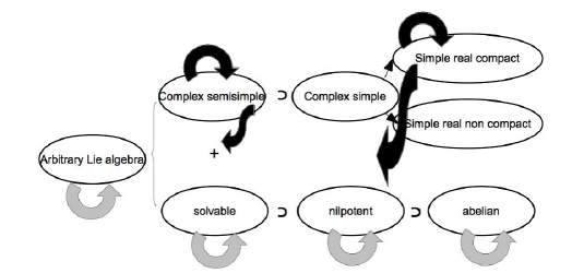
Figure 1: Action of the expansion methods on the scheme of the Theory of the Classification of Lie Algebras.

The Cartan decomposition of the expanded algebra was also obtained when the expansion preserves compactness. To check all these theoretical results, an example was given by studying all the possible expansions of the semisimple algebra $\mathfrak{sl}(2,\mathbb{R})$ with semigroups of order up to $6$. This checking was made with some computer programs that has been the starting point to construct the Java library that we will present in the next Sections. Before showing how the library is constructed and how it works, we give a brief review of the classification of semigroups.

2.4 Review of finite semigroups programs

Discrete semigroups have been a subject of intensive research in Mathematics and its classification have been made by many different authors (see e.g. [57, 60, 61, 62, 63, 64, 65, 66, 67, 68, 69] and references therein). In particular, the number of finite non-isomorphic semigroups of order $n$ is given in the following table:

order $$Q=\$$# semigroups

1 1

2 4

3 18

4 126 [Forsythe ’54]

5 1,160 [Motzkin, Selfridge ’55]

6 15,973 [Plemmons ’66]

7 836,021 [Jurgensen, Wick ’76]

8 1,843,120,128 [Satoh, Yama, Tokizawa ’94]

9 52,989,400,714,478 [Distler, Kelsey, Mitchell ’09]

10 12,418,001,077,381,302,684 [Distler, Jefferson, Kelsey, Kotthoff ’16]

   (27)

As shown in the table the problem of enumerating the all non-isomorphic finite semigroups of a certain order is a non-trivial problem. In fact, the number $Q$ of semigroups increases very quickly with the order of the semigroup. Since the original algorithms proposed by Plemmons [62, 57, 63] to computationally generate non isomorphic semigroups, a lot of work has been aided by computers. Remarkably, the order 9 has only been reached with the aid of supercomputers and the number (but not the explicit list of semigroup tables) for the order 10 has been obtained very recently [70].

Particularly, in Ref. [71] there were constructed very useful algorithms to make calculations with finite semigroups. First, the program gen.f generates in lexicographical ordering the lists of all the non-isomorphic semigroups of order $n=1,2,...,8$. This means that if we find a semigroup table $\tilde{S}$ which is not contained in one of those lists, then:

• $\tilde{S}$ does not have lexicographical ordering and

• $\tilde{S}$ is isomorphic to one and only one table of the lists generated by gen.f.

In each list, a semigroup $S_{\left(n\right)}^{a}$ of order $n$ is univocally identified by the number $a=1,...,Q$ and the semigroup elements are denoted by $\lambda_{\alpha}$ with $\alpha=1,...,n$.

The second program of Ref. [71] is com.f, which takes one of these lists generated by gen.f and selects only the abelian semigroups. For example, for $n=2$ the elements are labeled by $\left\{\lambda_{1},\lambda_{2}\right\}$ and the program com.f gives the following list of semigroups:

$$S_{\left(2\right)}^{1}$$

      ,

      ,

     (28)

Note that the semigroup $S_{\left(2\right)}^{3}$ is not given in the list (28) because it is not abelian. In the library that will described in the next section, it will be easier to use the full lists of semigroups generated by gen.f. When needed, we will select the abelian ones using a method similar to com.f.

2.5 Description of the library and notation

As a preliminar step, we have used the program gen.f of Ref. [71] to generate the files sem.2, sem.3, sem.4, sem.5 and sem.6 which contain all the non isomorphic semigroups up to order 6. As we will see, those files are the input data for many of our programs.

To use the Java library that we present in this work it is necessary to download the linear algebra package jama.jar from [72] and the following files from [56]:

File Brief description

data.zip Contains the the files sem.n

sexpansion.jar Is the library itself

examples.zip Example programs listed in Appendix A and explained in Section 5

Output_examples.zip Output samples of the example programs

   (29)

A ReadMe.pdf file is also provided with detailed installation instructions, should they be needed.

Our library is composed of the following classes (to see the source code unzip the file sexpansion.jar):

1. Semigroup.java

2. SetS.java

3. Selector.java

4. SelectorReduced.java

5. SelectorResonant.java

6. SelectorResonantReduced.java

7. StructureConstantSet.java

8. StructureConstantSetExpanded.java

9. StructureConstantSetExpandedReduced.java

10. StructureConstantSetExpandedResonant.java

11. StructureConstantSetExpandedResonantReduced.java

Each class contains different methods. A brief description can be found in the code at the beginning of each class and method. As the full documentation of the library is available in [73], in this article we will describe only the most important methods of these classes (see Sections 3-4).

In addition, there are 45 programs included as examples in the file examples.zip whose aim is to show how the methods of our library works. They are named with the prefixes I, II, III which stand for the following classification:

I    :  General computations with semigroups,

II   :  Examples of S-expansions of Lie algebras

III  :  Programs related with the calculations made in Ref. [55].

The list of these example programs is given in the Appendix A and most of them will be described in the section 5.

The type of resonances implemented on this first version

The methods that will be described in Sections 3 and 4, are able to work with algebras having a decomposition $\mathcal{G}=V_{0}\oplus V_{1}$ with the subspace structure given by

$$\left[V_{0},V_{0}\right] \subset V_{0}\,,$$

$$\left[V_{0},V_{1}\right] \subset V_{1}\,,$$

$$\left[V_{1},V_{1}\right] \subset V_{0}\,.$$ (30)

Correspondingly, the type of resonant decomposition that will be considered have the form $S=S_{0}\cup S_{1}$ and satisfy

$$S_{0}\times S_{0} \subset S_{0}\,,$$

$$S_{0}\times S_{1} \subset S_{1}\,,$$

$$S_{1}\times S_{1} \subset S_{0}\,.$$ (31)

Then, the resonant subalgebras that will be obtained have the form,

$$\mathcal{G}_{S,R}=\left(S_{0}\otimes V_{0}\right)\oplus\left(S_{1}\otimes V_{1}\right)\,.$$ (32)

We will also deal with the case in which the semigroup may have a $0_{S}$ element. Therefore, the library will allow us to extract from $\mathcal{G}_{S}$ the following three types of smaller algebras:

• Resonant subalgebras, when the original subalgebra has the subspace decomposition described in (30) and the semigroup posseses a resonant decomposition satisfying (31),

• $0_{S}$-Reduced algebras, when the semigroup has a $0_{S}$ element,

• $0_{S}$-Reduction of the resonant subalgebra when the semigroup has simultaneously a $0_{S}$ element and the resonant decomposition given by Eq. (31).

In a first stage, the situation described by Eqs. (30-32) (particular cases of Eqs. (14-16)), will be enough for the applications we want to consider in this work. However, as our library has an open GNU licence, we expect that it can be extended in order to perform S-expansions of algebras having more general subspace structures.

Conventions and notation

For programming language reasons, the semigroup elements $\lambda_{\alpha}$ must be labeled by their sub-index number,

$$\lambda_{\alpha}\longleftrightarrow\alpha\,,$$ (33)

with $\ \alpha=1,\ldots,n$. With this convention, the clousure is given by

$$\lambda_{\kappa\left(\alpha,\beta\right)}=\lambda_{\alpha}\cdot\lambda_{\beta}\longleftrightarrow\kappa\left(\alpha,\beta\right)=\alpha\cdot\beta\,$$ (34)

so that the multiplication table, Eq. (1), can be written as

$$A=\begin{pmatrix}a_{\alpha\beta}\end{pmatrix}\equiv\begin{pmatrix}\alpha\cdot\beta\end{pmatrix}\,.$$ (35)

Thus, properties like associative and commutativity respectively read,

$$\left(\alpha\cdot\beta\right)\cdot\gamma=\alpha\cdot\left(\beta\cdot\gamma\right)\ ,\ \ \alpha\cdot\beta=\beta\cdot\alpha\,,$$ (36)

which in terms of the multiplication table, can be expressed as

$$a_{a_{\alpha,\beta},\gamma}=a_{\alpha,a_{\beta,\gamma}}\ ,\ \ a_{\alpha\beta}=a_{\beta\alpha}\,.$$ (37)

An isomorphism, like the one described in Eq. (6), will be then denoted by

$$\left(\alpha_{1}\alpha_{2}\cdots\alpha_{n}\right)$$ (38)

and means: change $1$ by $\alpha_{1}$, change $2$ by $\alpha_{2}$, … and finally change $n$ by $\alpha_{n}$.

In the codes, latin characteres are used to label both semigroup elements and generators of the Lie algebra and its meaning is specified.

3 Methods for semigroups calculations

3.1 Loading all the non-isomorphic semigroups

Using the conventions and notations adopted in Section 2.5, we define the Semigroup class to represent a discrete semigroup and all the operations which can be performed with them.

⬇

public class Semigroup {

int[][] data;

int order;

int ID;

Obviously the code is bigger, but for space reasons we restrict ourselves only to describe the main parts of the methods and classes. Thus, we use 3 variables to save the information of a semigroup $S_{\left(n\right)}^{a}$: an integer ID which correspond to the identifier $a$ of the semigroup, a second integer order which tells us the order $n$ of the semigroup and a matrix of integers data where we save the multiplication table of the semigroup $A=\begin{pmatrix}a_{\alpha\beta}\end{pmatrix}\equiv\begin{pmatrix}\alpha\cdot\beta\end{pmatrix}$.

As explained in Section 2.5, in many of the calculations that will be done is necessary to load the semigroups generated by the program gen.f of Ref. [71]. This is done by the method loadFile which loads all the semigroups of a given order (up to order 6) returning us an array of Semigroup objects. To load all the avaliable semigroups from order 2 to 6 we use the method loadFromFile, which uses the method loadFile. In Section 5 we will show how the method loadFromFile is used in different problems.

3.2 Associativity, commutativity and $0_{S}$-element

To check if a given a multiplication table of a set of elements $S=\left\{{\alpha}\right\}_{\alpha=1}^{n}$ is a semigroup, we must check if it is associative. This means to check the relations $\left(\alpha\cdot\beta\right)\cdot\gamma=\alpha\cdot\left(\beta\cdot\gamma\right)$ for all $\alpha,\beta,\gamma=1,\ldots,n$. We perform this task with the method isAssociative.

⬇

public boolean isAssociative() {

int i , j , k ;

for ( i = 0 ; i < order ; ++ i) {

for ( j = 0 ; j < order ; ++j) {

for ( k = 0 ; k < order ; ++ k) {

if( ! (data[i][data[j][k]-1] == data[data[i][j]-1][k])) {

return false ;

}}}}

return true;

}

Basically, this method returns true if a given multiplication table is associative.

On the other hand, as described in section 2.2, to perform a S-expansion the semigroup used must be commutative. The method isCommutative returns true if a given semigroup is commutative, i.e., $\alpha\cdot\beta=\beta\cdot\alpha$.

⬇

public boolean isCommutative(){

int i, j;

for ( i = 0 ; i < order ; ++i) {

for( j = 0 ; j < order ; ++j ) {

if( ! (data[i][j] == data[j][i])) {

return false;

}}}

return true;

}

In section 2.2 we have explained that when a commutative semigroup has a zero element satisfying $\alpha\cdot 0_{S}=0_{S}\;\forall\alpha$ it is possible to perform a $0_{S}$-reduction of the expanded algebra. To be able to automatize that procedure we need a method which can look for the zero element for any semigroup. The method findZero gives the zero element when the semigroup does have it, otherwise it returns $-1$ as a result.

⬇

public int findZero() {

int i, j ;

boolean isZero = false ;

for ( i = 0 ; i < order ; ++ i ) {

if ( isZero == true ) {

return i ;

}

j = 0 ;

isZero = true;

while ( isZero && (j < order )) {

if ( data[j][i] != i+1) {

isZero = false ;

}

++j;

}}

if ( isZero == true ) {

return order ;

}

return -1 ;

}

On the other hand, it is also useful to have in some cases an auxiliar method to check for the equality of two given semigroups. The method isEqualTo returns true if they are equal.

⬇

public boolean isEqualTo ( Semigroup B ) {

int i,j;

if ( this.order != B.order ) {

return false;

}

for ( i = 0 ; i < this.order ; ++i ) {

for ( j = 0 ; j < B.order ; ++j) {

if ( this.data[i][j] != B.data[i][j]){

return false;

}}}

return true;

}

In Section 5 we will show how the methods loadFromFile, isAssociative, isCommutative, findZero and isEqualTo are used in different problems.

3.3 Creating sets and the permutation group $\Sigma_{n}$

As explained in section 2.1, the group of isomorphism of the semigroups or order $n$ is the group of permutations of $n$ elements, $\Sigma_{n}$. Thus, we define the SetS class to represent a permutation.

⬇

public class SetS {

int [] list ;

int nElements ;

A SetS object contains an integer nElements representing the number of elements to which we want to apply the permutation and a list where we save the permutation with the notation given in Eq. (38) in Section 2.5. This objects will also serve us to save any set of non repeated integers, like the one we will use for the resonant decomposition of a discrete semigroup.

Again, for space reasons, we are not able to reproduce the complete definition of the SetS class here and only its main methods will be described in what follows (remind that the full library is available on [56]).

To create a SetS object just from an array of integers we can use the code

⬇

public SetS( int [] elements ) {

list = elements ;

nElements = elements.length;

}

while to create a SetS of $n$ elements containing the identity permutation in $\Sigma_{n}$ we should use

⬇

public SetS( int n ){

nElements = n;

list = new int[n];

int i ;

for ( i = 0 ; i < n ; ++i) {

list[i] = i +1 ;

}}

Now, to check if two given semigroups are isomorphic we have to try all the existent isormorphisms for a given order. This means to use all the elements in $\Sigma_{n}$. This is performed by the method allPermutations, which returns an array of SetS objects containing all the elements in $\Sigma_{n}$.

⬇

SetS [] allPermutations( ) {

SetS result = new SetS(0) ;

return this.permutationsAux( this , result);

}

This method uses the auxiliar method permutationsAux, which actually performs most of the work. This is a recursive method which takes an original SetS object and reorders its elements in all the possible ways. This is, given the identity permutation

$$\left(1\,2\,\cdots\,n\right)$$

it returns all the possible ways to permute it, i.e., all the elements of the permutation group $\Sigma_{n}$. As we can see in what follows, permutationsAux uses the methods addElement and eraseElement whose definition is obvious and we do not reproduce here.

⬇

SetS [] permutationsAux( SetS original, SetS result ) {

int i , j;

SetS original2 , result2 ;

SetS [] list = null;

SetS [] totalList = null;

SetS [] previousList = null;

int N = 0 ;

if ( original.nElements == 0 ) {

list = new SetS[1];

list[0] = result ;

return list ;

}

for ( i = 0 ; i < original.nElements ; i++ ){

result2 = result.addElement( original.elementAt(i) ) ;

original2 = original.eraseElement(i) ;

list = permutationsAux( original2 , result2) ;

N = N + list.length ;

previousList = totalList ;

totalList = new SetS[N];

for ( j = 0 ; j < N - list.length ; ++j) {

totalList[j] = previousList[j];

}

for ( j = 0 ; j < list.length ; ++j) {

totalList[ j + N - list.length ] = list[j];

}}

return totalList;

}

As explained in section 2.1, two given semigroups are isomorphic or anti-isomorphic if there exist a permutation $\sigma\in\Sigma_{n}$ that relates them through the Eqs. (7) and (8). Here we will describe two basic operations related with isomorphisms. First, the method which applies a given isormorphism to a semigroup is permuteWith:

⬇

public Semigroup permuteWith( SetS s ) {

int i,j;

int [][] matrix = new int[this.order][ this.order];

SetS inverse = s.inversePermutation() ;

for ( i = 0 ; i < this.order ; ++i) {

for ( j = 0 ; j < this.order ; ++j) {

matrix[i][j] = this.data[ inverse.elementAt(i) - 1]

[ inverse.elementAt(j) -1] ;

}}

for ( i = 0 ; i < this.order ; ++i) {

for ( j = 0 ; j < this.order ; ++j) {

if ( matrix[i][j] != -1 ) {

matrix[i][j] = s.elementAt( matrix[i][j] - 1 );

}}}

return new Semigroup(matrix);

}

In other cases, what we need is finding all the isomorphic forms of a given semigroup, i.e., apply all the possible permutations to a given semigroup. In that case, we use the method permute, which returns an array of Semigroup objects containing all the permutations of a given one:

⬇

public Semigroup [] permute() {

SetS identity = new SetS( this.order );

SetS [] permutations = identity.allPermutations() ;

int k;

Semigroup [] result = new Semigroup [permutations.length];

for ( k = 0 ; k < permutations.length ; ++k) {

result[k ] = this.permuteWith(permutations[k]);

}

return result;

}

Then, a simple method to check anti-isomorphisms is given by

⬇

public Semigroup [] antiPermute () {

return (this.transpose()).permute( );

}

In Section 5 we will show different examples using these methods.

3.4 Resonant decompositions

In Section 2.2 we explained that a resonant subalgebra can be extracted from the expanded algebra $\mathcal{G}_{S}$ when the original algebra has a certain subspace structure and the semigroup satisfy a so called resonant decomposition (see Eqs. (14-15)). As mentioned in Section 2.5, for our pourpuses it will be enough to consider the case given by Eqs.(30-31), i.e., we will study resonant conditions of the type,

$$S_{0}\cdot S_{0}\subset S_{0}\,,$$

$$S_{0}\cdot S_{1}\subset S_{1}\,,$$

$$S_{1}\cdot S_{1}\subset S_{0}\,.$$

A previous step to check if two given subsets $S_{0}$ and $S_{1}$ satisfy the resonance condition, is to check that their union reproduce the full semigroup, i.e. $S_{0}\cup S_{1}=S$. This is done by the method fillTheSpace of the SetS class.

⬇

public static boolean fillTheSpace(SetS s1,SetS s2,int order){

int i ;

for ( i = 0 ; i < order ; ++i) {

if ( ! s1.find( i+1) && ! s2.find(i +1) ){

return false;

}}

return true;

}

The parameter order tells the method the order of the semigroup for which s1 and s2 must be a resonant decomposition.

The method isResonant returns true if the two SetS objects s0 and s1 represent a resonant decomposition for the current Semigroup object.

⬇

public boolean isResonant( SetS s0 , SetS s1) {

int i,j, n0 = s0.nElements, n1 = s1.nElements ;

if ( SetS.fillTheSpace(s0, s1, order) ) {

for ( i = 0 ; i < n0 ; ++i ) {

for ( j = 0 ; j < n0 ; ++j ) {

if ( ! s0.find(this.data[s0.elementAt(i) -1]

[s0.elementAt(j)-1] ) ) {

return false ;

}}}

for ( i = 0 ; i < n0 ; ++i ){

for ( j = 0 ; j < n1 ; ++j) {

if ( ! s1.find( this.data[s0.elementAt(i)-1]

[s1.elementAt(j)-1])) {

return false;

}}}

for ( i = 0 ; i < n1 ; ++i) {

for ( j = 0 ; j < n1 ; ++j) {

if (! s0.find( this.data[s1.elementAt(i)-1]

[s1.elementAt(j)-1])) {

return false;

}}}}

else {

return false;

}

return true;

}

Once we are able to check is a given decomposition of a semigroup is resonant, we want to be able to look for resonant decompositions. The method findResonances looks for all the possible resonances of a semigroup, with $S_{0}$ and $S_{1}$ having respectively n1 and n2 elements.

⬇

public SetS [][] findResonances( int n1, int n2 ) {

SetS total = new SetS(this.order) ;

SetS [] list1 = total.subSets(n1) ;

SetS [] list2 = total.subSets(n2) ;

SetS [][] result = null;

SetS [][] auxiliar = null ;

int foundResonances = 0 ;

int i , j , k = 0;

for ( i = 0 ; i < list1.length ; ++ i ) {

for ( j = 0 ; j < list2.length ; ++j ) {

if ( this.isResonant( list1[i], list2[j])

&& SetS.fillTheSpace( list1[i], list2[j], this.order)) {

foundResonances = foundResonances + 1 ;

auxiliar = result ;

result = new SetS[foundResonances ] [2] ;

for ( k = 0 ; k < foundResonances -1 ; ++k) {

result[k][0] = auxiliar[k][0];

result[k][1] = auxiliar[k][1];

}

result[ foundResonances - 1 ] [0] = list1[i];

result[ foundResonances - 1] [1] = list2[j];

}}}

return result;

}

In case it finds any resonant decomposition, this method returns a 2 dimensional array whose element $result[i][0]$ is the $S_{0}$ and $result[i][1]$ is $S_{1}$ for the ith decomposition found. This method uses the auxiliar method subSets which returns all the subsets with $n$ element of a given SetS object.

⬇

public SetS [] subSets( int n ) {

SetS result = new SetS();

return SetS.cleanDuplicates(auxSubset( this , result, n ));

}

This method is just a more convenient way to use the recursive method auxSubset:

⬇

public SetS[] auxSubset( SetS original , SetS result, int n) {

int i;

SetS [] list = null;

SetS [] totalList = null;

if ( n == 0 ) {

totalList = new SetS[1];

totalList[0] = result;

return totalList ;

}

SetS aux1;

SetS aux2;

for ( i = 0 ; i < original.nElements ; ++i ) {

aux1= original.eraseElement(i);

aux2= result.addElement( original.elementAt(i));

list = auxSubset(aux1 , aux2 , n-1);

totalList = SetS.add(list , totalList );

if ( totalList != null ) {

}}

return totalList ;

}

The auxiliar method cleanDuplicates just cleans possible duplicates in an array of SetS objects

⬇

public static SetS[] cleanDuplicates( SetS [] lst) {

int i, j ;

int n = lst.length ;

int elements = n;

SetS [] newList ;

for ( i = 0 ; i < n ; ++i) {

lst[i] = SetS.sort(lst[i]);

}

for ( i = 0 ; i < n ; ++i) {

for ( j = i +1 ; j < n ; ++j){

if (lst[i] != null && lst[j] != null && lst[i].equalTo(lst[j])){

lst[j] = null ;

elements = elements - 1 ;

}}}

newList = new SetS[elements] ;

j = 0 ;

for ( i = 0 ; i < n ; ++i) {

if ( lst[i] != null ) {

newList[j] = lst[i];

++j;

}}

return newList ;

}

To find all the possible resonant decompositions of a given semigroup we define the method findAllResonances

⬇

public SetS [][] findAllResonances() {

int i , j , k;

SetS [][] result = null;

SetS [][] auxiliar ;

SetS [][] intermediateResult;

int N = 0;

for ( i = 1 ; i < this.order ; ++i) {

for ( j = 1 ; j < this.order ; ++j) {

intermediateResult = this.findResonances( i, j) ;

if ( intermediateResult != null ) {

auxiliar = result ;

N = N + intermediateResult.length ;

result = new SetS[ N][2];

for ( k = 0 ; k < N - intermediateResult.length ; ++k ) {

result[k][0] = auxiliar[k][0];

result[k][1] = auxiliar[k][1];

}

for ( k = 0 ; k < intermediateResult.length ; ++k) {

result[ N - intermediateResult.length + k][0 ] =

intermediateResult[k][0];

result[ N - intermediateResult.length + k][ 1 ] =

intermediateResult[k][1];

}}}}

return result;

}

In the following Sections we will see the usefulness of these methods.

4 Methods for S-expansions

In this Section we will explain the construction of the classes which will allow us to:

• Represent a semigroup of order $n$ and compute the metric $\mathbf{g}^{S}$ defined in Eq. (23)),

• Represent Lie algebras in terms of its structure constants (adjoint representation) and compute the Killing-Cartan (KC) $\mathbf{g}$ metric defined in Eq. (24),

• Show the selector in a fancy way, by using $n$ boxes of dimension $n\times n$, so the component $K_{ab}^{c}$ is found in box $a$, row $b$, column $c$ (and do something similar for the structure constants of the original and expanded algebras),

• Obtain the S-expanded algebra, resonant subalgebra, $0_{S}$-reduced algebra and the $0_{S}$-reduction of a resonant subalgebra,

• Compute the KC metric of the original Lie algebra, the S-expanded algebra, the resonant subalgebra, the $0_{S}$-reduced algebra and the $0_{S}$-reduction of a resonant subalgebra (see Eqs. (26) and Section 3.2 of Ref. [55])

A reminder:

For space reasons, we will only explain the main parts of those classes here. The full source code of the library is available in [56] and its documentation can be found in [73].

4.1 Representing semigroups and Lie algebras

In section 2.1 it was shown that an informal but useful way to represent the multiplication law of a semigroup is by means of the selectors $K_{\alpha\beta}^{\kappa}$, whose definition was given in Eq. (3). Thus, we define the Selector class to represent these quantities.

⬇

public class Selector {

int order ;

int [][][] data ;

It has 2 variables: an integer to save the order of the semigroup and an array to save all the selectors in the semigroup as follows

$$\mathrm{data}[a][b][c]\equiv K_{ab}^{c}\,.$$

The methods Selector, SetS and get allow to create a selector object for a semigroup of order $n$, to set and return the value of the $K_{ab}^{c}$ component of the selector. The method show gives the selector by means of $n$ boxes of dimension $n\times n$, so the component $K_{ab}^{c}$ is found in box $a$, row $b$, column $c$. According to Eq. (4), this means that box $a$ is indeed the adjoint representation of the element $\lambda_{a}$.

For example, consider the following semigroup,

λ1λ1λ2λ3λ4λ2λ2λ3λ4λ4λ3λ3λ4λ4λ4λ4λ4λ4λ4λ4.fragments fragmentsλ1fragmentsλ1fragmentsλ2fragmentsλ3fragmentsλ4fragmentsλ2fragmentsλ2fragmentsλ3fragmentsλ4fragmentsλ4fragmentsλ3fragmentsλ3fragmentsλ4fragmentsλ4fragmentsλ4fragmentsλ4fragmentsλ4fragmentsλ4fragmentsλ4fragmentsλ4\begin{tabular}[c]{l|llll}&$\lambda_{1}$&$\lambda_{2}$&$\lambda_{3}$&$\lambda_{4}$\\ \hline\cr$\lambda_{1}$&$\lambda_{1}$&$\lambda_{2}$&$\lambda_{3}$&$\lambda_{4}$\\ $\lambda_{2}$&$\lambda_{2}$&$\lambda_{3}$&$\lambda_{4}$&$\lambda_{4}$\\ $\lambda_{3}$&$\lambda_{3}$&$\lambda_{4}$&$\lambda_{4}$&$\lambda_{4}$\\ $\lambda_{4}$&$\lambda_{4}$&$\lambda_{4}$&$\lambda_{4}$&$\lambda_{4}$\end{tabular}\,.

λ1λ2λ3λ4λ1λ2λ3λ4 (39)

The following piece of code (part of the program 26 in Appendix A) ilustrates how the Selector class works together with the method getSelector of the Semigroup class, to build and print a selector object for this semigroup.

⬇

int [][] mS = {{1,2,3,4},{2,3,4,4},{3,4,4,4}, {4,4,4,4}};

Semigroup S = new Semigroup(mS) ;

Selector Adj = S.getSelector() ;

Adj.show();

The output reads,

For the considered semigroup of order m, here we print the m matrices K_{a,b}^{c}=M_{b,c}
(with a=1,...,m) which gives the adjoint representation for the elements of the semigroup.
*********
Adj [lambda_{1}] = ( K_{1,b}^{c} ) =
 1 0 0 0
 0 1 0 0
 0 0 1 0
 0 0 0 1
*********
Adj [lambda_{2}] = ( K_{2,b}^{c} ) =
 0 1 0 0
 0 0 1 0
 0 0 0 1
 0 0 0 1
*********
Adj [lambda_{3}] = ( K_{3,b}^{c} ) =
 0 0 1 0
 0 0 0 1
 0 0 0 1
 0 0 0 1
*********
Adj [lambda_{4}] = ( K_{4,b}^{c} ) =
 0 0 0 1
 0 0 0 1
 0 0 0 1
 0 0 0 1

This class also contains the methods selectorMetric and expandedMetric which computes the metrics $\mathbf{g}^{S}$ and $\mathbf{g}^{E}$ defined in Eqs. (23-25). Explicit examples with them will be given in Section 5.5.

In a similar way we construct the classes SelectorReduced, SelectorResonant and SelectorResonantReduced, which extend the Selector class for the cases where the semigroup have a zero element, a resonance and both simultaneously.

On the other hand, to represent a Lie algebra by means of its structure constants we define the StructureConstantSet class.

⬇

public class StructureConstantSet {

double [][][] constants ;

int N ;

The integer $N$ is the number of generators of the Lie algebra and, with the convention

$$\left[X_{i},X_{j}\right]=C_{ij}^{k}X_{k}\,,$$

we choose

$$\mathrm{constants}[i][j][k]\equiv C_{ij}^{k}\,.$$

This class contains methods that allow to introduce the values of the structure constants and show them in a similar way as was done for the selectors. In particular, the following method sets the values of $C_{ij}^{k}$ and $C_{ji}^{k}$.

⬇

public void setStructureConstant(int i, int j, int k, double fijk){

constants[i][j][k] = fijk ;

constants[j][i][k] = - fijk;

}

As the first possition of an array [ ] is usually [0], the method setStructureConstant must be used to introduce the non-vanishing structure constants $C_{ij}^{k}$ as:

⬇

NameOfTheAlgebra.setStructureConstant(i, j, k, value of C_{ij}^{k})

where $i,j,k=0,1,\ldots,N-1$. However, the outputs will be usually given in such a way that $i,j,k=1,\ldots,N$ .

As an example, the following piece of code (also part of the program 26 in Appendix A) ilustrates how to introduce the structure constants of the $\mathfrak{sl}(2)$ algebra,

$$\left[X_{1},X_{2}\right]=-2X_{3}$$

$$\left[X_{1},X_{3}\right]=2X_{2}$$

$$\left[X_{2},X_{3}\right]=2X_{1}\,,$$ (40)

in order to obtain its adjoint representation.

⬇

sl2.setStructureConstant(0, 1, 2, -2);

sl2.setStructureConstant(0, 2, 1, 2);

sl2.setStructureConstant(1, 2, 0, 2);

sl2.show();

The output reads,

For the considered Lie algebra of dimension n, we print the n matrices C_{ij}^{k}=M_{jk}
(with i=1,...,n) which gives the adjoint representation for the elements of the algebra.
*********
Adj [ X_{1} ] = ( C_{1,j}^{k} ) =
 0.0  0.0  0.0
 0.0  0.0 -2.0
 0.0  2.0  0.0
*****
*********
Adj [ X_{2} ] = ( C_{2,j}^{k} ) =
 0.0  0.0  2.0
 0.0  0.0  0.0
 2.0  0.0  0.0
*****
*********
Adj [ X_{3} ] = ( C_{3,j}^{k} ) =
 0.0 -2.0  0.0
-2.0  0.0  0.0
 0.0  0.0  0.0

Several simple operations can be perfomed by the methods of the StructureConstantSet class. For example, the following one computes the Killing-Cartán metric of a given Lie algebra.

⬇

public Matrix cartanKillingMetric(){

int i, j , k, l;

double sum = 0 ;

double [][] metric = new double[N][N] ;

for ( i = 0 ; i < N ; ++i) {

for ( j = 0 ; j < N ; ++j ) {

sum = 0 ;

for ( k = 0 ; k < N ; ++k ) {

for ( l = 0 ; l < N ; ++l ) {

sum = sum + this.structureConstant(i,k,l)

* this.structureConstant(j,l,k);

}}

metric[i][j] = sum ;

}}

return new Matrix( metric );

}

Explicit examples using this and other methods included in the classes Selector, StructureConstantSet will be given in Section 5.5.

4.2 The S-expanded algebra

In double index notation, the Lie bracket of the S-expanded algebra is written here as

$$\left[X_{\left(i,a\right)},X_{\left(j,b\right)}\right]=C_{ij}^{k}K_{ab}^{c}X_{\left(k,c\right)}\,.$$

To use this double index notation internally in our library, we create the class StructureConstantSetExpanded.

⬇

public class StructureConstantSetExpanded {

int n,m ;

double [][][][][][] data ;

Thus, an object of this class has information about the dimension $n$ of the original Lie algebra, the order $m$ of the semigroup used to perform the S-expansion and uses the 6-dimensional array data to save the structure constants, in such a way that

$$\mathrm{data}[i][a][j][b][k][c]\equiv C_{(i,a)(j,b)}^{(k,c)}\,.$$

To get the S-expanded algebra we must follow the next steps:

1. Create a StructureConstantSet object to store the original Lie algebra,

2. Create a Semigroup object S to store the semigroup which we want to use for the S-expansion,

3. Use the method getExpandedStructureConstant to perform the S-expansion of the Lie algebra with the semigroup object,

4. Use the method showCommut to get the non vanishing commutators of the expanded algebra $\mathcal{G}_{S}$,

5. Use the method showSC to get the non vanishing structure constants of $\mathcal{G}_{S}$,

6. Use the method cartanKillingMetric to compute the KC metric of $\mathcal{G}_{S}$.

A piece of code performing the steps above for the algebra and the semigroup given by Eqs. (40) and (39), would be

⬇

StructureConstantSet sl2 = new StructureConstantSet(3) ;

sl2.setStructureConstant(0, 1, 2,-2) ;

sl2.setStructureConstant(0, 2, 1, 2) ;

sl2.setStructureConstant(1, 2, 0, 2) ;

int [][] SemigroupTable = {{1,2,3,4},{2,3,4,4},{3,4,4,4}, {4,4,4,4}};

Semigroup S = new Semigroup(SemigroupTable) ;

StructureConstantSetExpanded Gexp = S.getExpandedStructureConstant(sl2);

Gexp.showCommut();

Gexp.showSC();

Matrix metricaGexp = Gexp.cartanKillingMetric();

metricaGexp.print(0,0);

Further examples with sample outputs will be given in Section 5.5.

4.3 The resonant subalgebra

To get a resonant subalgebra of a S-expanded algebra, we define the StructureConstantSetExpandedResonant class, which is a child of the StructureConstantSetExpanded class.

⬇

public class StructureConstantSetExpandedResonant extends

StructureConstantSetExpanded {

SetS S0, S1, V0, V1;

Here S0 and S1 represent the resonant decomposition of the semigroup, whilst V0 and V1 give the graded decomposition of the Lie algebra. To get the resonant subalgebra of an S-expanded algebra we must

1. Get the correspondent S-expanded algebra, following the steps in the previous section,

2. Introduce the resonant decomposition $S_{0}$ and $S_{1}$ with the method SetS,

3. Introduce the graded decomposition $V_{0}$ and $V_{1}$ also with the method SetS,

4. Use all these objects to create a StructureConstantSetExpandedResonant object,

5. Use methods showCommutRes, showSCRes and cartanKillingMetricPretty to obtain the non vanishing commutators, structure constants and KC metric of the resonant subalgebra.

For example, the algebra considered in Eq. (40) has a subspace decomposition given by $\mathfrak{sl}(2)=V_{0}\oplus V_{1}$ , where

$$V_{0}=\{X_{1}\}\text{ and }V_{1}=\{X_{2},X_{3}\}\,.$$

Considering again the semigroup given in Eq. (39), we see that admits a decomposition $S=S_{0}\cup S_{1}$ with

$$S_{0}=\{1,3,4\}\text{ and }S_{1}=\{2,4\}\,,$$

which is resonant, i.e., it satisfies Eq. (31). Thus, the following piece of code perform the S-expansion of $\mathfrak{sl}(2)$ and it calculates the resonant subalgebra.

⬇

StructureConstantSet sl2 = new StructureConstantSet(3) ;

sl2.setStructureConstant(0, 1, 2,-2) ;

sl2.setStructureConstant(0, 2, 1, 2) ;

sl2.setStructureConstant(1, 2, 0, 2) ;

int [][] SemigroupTable = {{1,2,3,4},{2,3,4,4},{3,4,4,4}, {4,4,4,4}};

Semigroup S = new Semigroup(SemigroupTable) ;

int[] mS0 = {1,3,4} ;

SetS S0 = new SetS(mS0) ;

int[] mS1 = {2,4} ;

SetS S1 = new SetS(mS1) ;

int[] mV0 = {1};

SetS V0 = new SetS(mV0);

int[] mV1 = {2,3};

SetS V1 = new SetS(mV1);

StructureConstantSetExpanded Gexp = S.getExpandedStructureConstant(sl2);

StructureConstantSetExpandedResonant ResGexp =

new StructureConstantSetExpandedResonant(Gexp.data,S0,S1,V0,V1) ;

ResGexp.showCommutRes();

ResGexp.showSCRes();

Matrix metricaResGexp = ResGexp.cartanKillingMetricPretty();

metricaResGexp.print(0,0);

Other examples with samples of their outputs will be described in detail in Section 5.5.

4.4 S-expanded algebra followed by a $0_{S}$-reduction

To perform the reduction by the zero element of a S-expanded Lie algebra we define the StructureConstantSetExpandedReduced class, which is a child of the StructureConstantSetExpanded class.

⬇

public class StructureConstantSetExpandedReduced extends

StructureConstantSetExpanded {

int zero ;

Respect to the StructureConstantSetExpanded class, it only adds an integer variable to save the zero element.

What we need to perform the reduction by zero of a S-expanded algebra we have to

1. Get the S-expanded algebra in a StructureConstantSetExpanded,

2. Use it to create a StructureConstantSetExpandedReduced,

3. Use other methods in the class to obtain the non vanishing commutators, structure constants and KC metric of the reduced algebra.

For example, the semigroup given by Eq. (39) has $\lambda_{4}$ as the zero element. Thus, the following piece of code calculates the $0_{S}$-reduction of the S-expansion of the algebra $\mathfrak{sl}(2)$.

⬇

StructureConstantSet sl2 = new StructureConstantSet(3) ;

sl2.setStructureConstant(0, 1, 2,-2) ;

sl2.setStructureConstant(0, 2, 1, 2) ;

sl2.setStructureConstant(1, 2, 0, 2) ;

int [][] SemigroupTable = {{1,2,3,4},{2,3,4,4},{3,4,4,4}, {4,4,4,4}};

Semigroup S = new Semigroup(SemigroupTable);

StructureConstantSetExpandedReduced RedGexp =

new StructureConstantSetExpandedReduced

(S.getExpandedStructureConstant(sl2).data,4);

RedGexp.showCommutRed();

RedGexp.showSCRed();

Matrix metricaRedGexp = RedGexp.cartanKillingMetricPretty();

metricaRedGexp.print(0,0);

4.5 Resonant subalgebra followed by a $0_{S}$-reduction

We define the class StructureConstantSetExpandedResonantReduced, which is a child of the class StructureConstantSetExpandedResonant.

⬇

public class StructureConstantSetExpandedResonantReduced

extends StructureConstantSetExpandedResonant {

int zero;

We just add an integer to save the zero element. Its use is analogous to that of the StructureConstantSetExpandedResonant described in Section 4.3. Explicit examples using this class and its methods are given in Section 5.5.

5 Applications

Here we will describe most of the programs listed in Appendix A in order to show explicitly the kind of calculations that can be done with the methods described in the sections 3 and 4. Mainly, we will explain the ones that allow us to:

• Check associativity and commutativity, find the zero element and resonances for any given multiplication table,

• Apply permutations and find isomorphisms between any set of semigroups,

• Perform S-expansions with any given semigroup and, if the semigroup fulfills the necessary conditions, to find the resonant subalgebra $\mathcal{G}_{S,R}$, the reduced algebra $\mathcal{G}_{S,\text{red}}$ and the reduction of the resonant subalgebra $\mathcal{G}_{S,R,\text{red}}$,

• Identify S-expansions preserving semisimplicity.

With these examples the user can easily create new programs to perform his own calculations. Along this section, we will refer to the example programs by their Appendix-A number. When the output is short, the results are direclty printed to screen. Longer outputs are printed in .txt-files in the folder “./Output_examples/”, with the naming convention: Output_ + name of the program. In addition, most of the outputs can be found in the file Output_examples.zip available in [56]. Finally, we remind that a brief description about the general structure of these programs can be found in Section 2.5.

5.1 Examples of associativity and commutativity

The first two programs listed in Appendix A allow to check the associativity and commutativity of the following multiplication tables:

λ1λ1λ2λ3λ2λ2λ1λ2λ3λ3λ2λ1, λ1λ1λ1λ1λ2λ1λ2λ3λ3λ1λ1λ1, λ1λ1λ1λ3λ2λ1λ2λ3λ3λ3λ3λ1,fragments fragmentsλ1fragmentsλ1fragmentsλ2fragmentsλ3fragmentsλ2fragmentsλ2fragmentsλ1fragmentsλ2fragmentsλ3fragmentsλ3fragmentsλ2fragmentsλ1fragments fragmentsλ1fragmentsλ1fragmentsλ1fragmentsλ1fragmentsλ2fragmentsλ1fragmentsλ2fragmentsλ3fragmentsλ3fragmentsλ1fragmentsλ1fragmentsλ1fragments fragmentsλ1fragmentsλ1fragmentsλ1fragmentsλ3fragmentsλ2fragmentsλ1fragmentsλ2fragmentsλ3fragmentsλ3fragmentsλ3fragmentsλ3fragmentsλ1\begin{tabular}[c]{l|lll}$S_{\text{ex1}}$&$\lambda_{1}$&$\lambda_{2}$&$\lambda_{3}$\\ \hline\cr$\lambda_{1}$&$\lambda_{1}$&$\lambda_{2}$&$\lambda_{3}$\\ $\lambda_{2}$&$\lambda_{2}$&$\lambda_{1}$&$\lambda_{2}$\\ $\lambda_{3}$&$\lambda_{3}$&$\lambda_{2}$&$\lambda_{1}$\end{tabular}\,,\ \ \begin{tabular}[c]{l|lll}$S_{\text{ex2}}$&$\lambda_{1}$&$\lambda_{2}$&$\lambda_{3}$\\ \hline\cr$\lambda_{1}$&$\lambda_{1}$&$\lambda_{1}$&$\lambda_{1}$\\ $\lambda_{2}$&$\lambda_{1}$&$\lambda_{2}$&$\lambda_{3}$\\ $\lambda_{3}$&$\lambda_{1}$&$\lambda_{1}$&$\lambda_{1}$\end{tabular}\,,\ \ \begin{tabular}[c]{l|lll}$S_{\text{ex3}}$&$\lambda_{1}$&$\lambda_{2}$&$\lambda_{3}$\\ \hline\cr$\lambda_{1}$&$\lambda_{1}$&$\lambda_{1}$&$\lambda_{3}$\\ $\lambda_{2}$&$\lambda_{1}$&$\lambda_{2}$&$\lambda_{3}$\\ $\lambda_{3}$&$\lambda_{3}$&$\lambda_{3}$&$\lambda_{1}$\end{tabular}\,,

Sex1λ1λ2λ3Sex2λ1λ2λ3Sex3λ1λ2λ3Sex1λ1λ2λ3Sex2λ1λ2λ3Sex3λ1λ2λ3

λ1λ1λ2λ3λ4λ2λ2λ3λ4λ1λ3λ3λ4λ1λ2λ4λ4λ1λ2λ3, λ1λ5λ4λ2λ1λ3λ2λ4λ3λ5λ2λ1λ3λ2λ5λ1λ3λ4λ4λ1λ2λ3λ4λ5λ5λ3λ1λ4λ5λ2,fragments fragmentsλ1fragmentsλ1fragmentsλ2fragmentsλ3fragmentsλ4fragmentsλ2fragmentsλ2fragmentsλ3fragmentsλ4fragmentsλ1fragmentsλ3fragmentsλ3fragmentsλ4fragmentsλ1fragmentsλ2fragmentsλ4fragmentsλ4fragmentsλ1fragmentsλ2fragmentsλ3fragments fragmentsλ1fragmentsλ5fragmentsλ4fragmentsλ2fragmentsλ1fragmentsλ3fragmentsλ2fragmentsλ4fragmentsλ3fragmentsλ5fragmentsλ2fragmentsλ1fragmentsλ3fragmentsλ2fragmentsλ5fragmentsλ1fragmentsλ3fragmentsλ4fragmentsλ4fragmentsλ1fragmentsλ2fragmentsλ3fragmentsλ4fragmentsλ5fragmentsλ5fragmentsλ3fragmentsλ1fragmentsλ4fragmentsλ5fragmentsλ2\begin{tabular}[c]{l|llll}$S_{\text{ex4}}$&$\lambda_{1}$&$\lambda_{2}$&$\lambda_{3}$&$\lambda_{4}$\\ \hline\cr$\lambda_{1}$&$\lambda_{1}$&$\lambda_{2}$&$\lambda_{3}$&$\lambda_{4}$\\ $\lambda_{2}$&$\lambda_{2}$&$\lambda_{3}$&$\lambda_{4}$&$\lambda_{1}$\\ $\lambda_{3}$&$\lambda_{3}$&$\lambda_{4}$&$\lambda_{1}$&$\lambda_{2}$\\ $\lambda_{4}$&$\lambda_{4}$&$\lambda_{1}$&$\lambda_{2}$&$\lambda_{3}$\end{tabular}\,,\ \ \begin{tabular}[c]{l|lllll}$S_{\text{ex5}}$&$\lambda_{1}$&$\lambda_{2}$&$\lambda_{3}$&$\lambda_{4}$&$\lambda_{5}$\\ \hline\cr$\lambda_{1}$&$\lambda_{5}$&$\lambda_{4}$&$\lambda_{2}$&$\lambda_{1}$&$\lambda_{3}$\\ $\lambda_{2}$&$\lambda_{4}$&$\lambda_{3}$&$\lambda_{5}$&$\lambda_{2}$&$\lambda_{1}$\\ $\lambda_{3}$&$\lambda_{2}$&$\lambda_{5}$&$\lambda_{1}$&$\lambda_{3}$&$\lambda_{4}$\\ $\lambda_{4}$&$\lambda_{1}$&$\lambda_{2}$&$\lambda_{3}$&$\lambda_{4}$&$\lambda_{5}$\\ $\lambda_{5}$&$\lambda_{3}$&$\lambda_{1}$&$\lambda_{4}$&$\lambda_{5}$&$\lambda_{2}$\end{tabular}\,,

Sex4λ1λ2λ3λ4Sex5λ1λ2λ3λ4λ5Sex4λ1λ2λ3λ4Sex5λ1λ2λ3λ4λ5

λ1λ1λ1λ1λ1λ5λ5λ1λ1λ5λ5λ2λ1λ2λ1λ1λ5λ5λ1λ1λ5λ5λ3λ3λ3λ3λ3λ6λ6λ3λ3λ6λ6λ4λ3λ3λ3λ4λ6λ6λ3λ3λ6λ6λ5λ1λ1λ1λ1λ5λ5λ5λ5λ1λ1λ6λ3λ3λ3λ3λ6λ6λ6λ6λ3λ3λ7λ1λ1λ3λ3λ5λ6λ7λ8λ9λ10λ8λ1λ1λ3λ3λ5λ6λ8λ7λ10λ9λ9λ3λ3λ1λ1λ6λ5λ9λ10λ8λ7λ10λ3λ3λ1λ1λ6λ5λ10λ9λ7λ8.fragments fragmentsλ1fragmentsλ1fragmentsλ1fragmentsλ1fragmentsλ1fragmentsλ5fragmentsλ5fragmentsλ1fragmentsλ1fragmentsλ5fragmentsλ5fragmentsλ2fragmentsλ1fragmentsλ2fragmentsλ1fragmentsλ1fragmentsλ5fragmentsλ5fragmentsλ1fragmentsλ1fragmentsλ5fragmentsλ5fragmentsλ3fragmentsλ3fragmentsλ3fragmentsλ3fragmentsλ3fragmentsλ6fragmentsλ6fragmentsλ3fragmentsλ3fragmentsλ6fragmentsλ6fragmentsλ4fragmentsλ3fragmentsλ3fragmentsλ3fragmentsλ4fragmentsλ6fragmentsλ6fragmentsλ3fragmentsλ3fragmentsλ6fragmentsλ6fragmentsλ5fragmentsλ1fragmentsλ1fragmentsλ1fragmentsλ1fragmentsλ5fragmentsλ5fragmentsλ5fragmentsλ5fragmentsλ1fragmentsλ1fragmentsλ6fragmentsλ3fragmentsλ3fragmentsλ3fragmentsλ3fragmentsλ6fragmentsλ6fragmentsλ6fragmentsλ6fragmentsλ3fragmentsλ3fragmentsλ7fragmentsλ1fragmentsλ1fragmentsλ3fragmentsλ3fragmentsλ5fragmentsλ6fragmentsλ7fragmentsλ8fragmentsλ9fragmentsλ10fragmentsλ8fragmentsλ1fragmentsλ1fragmentsλ3fragmentsλ3fragmentsλ5fragmentsλ6fragmentsλ8fragmentsλ7fragmentsλ10fragmentsλ9fragmentsλ9fragmentsλ3fragmentsλ3fragmentsλ1fragmentsλ1fragmentsλ6fragmentsλ5fragmentsλ9fragmentsλ10fragmentsλ8fragmentsλ7fragmentsλ10fragmentsλ3fragmentsλ3fragmentsλ1fragmentsλ1fragmentsλ6fragmentsλ5fragmentsλ10fragmentsλ9fragmentsλ7fragmentsλ8\begin{tabular}[c]{l|llllllllll}$S_{\text{ex6}}$&$\lambda_{1}$&$\lambda_{2}$&$\lambda_{3}$&$\lambda_{4}$&$\lambda_{5}$&$\lambda_{6}$&$\lambda_{7}$&$\lambda_{8}$&$\lambda_{9}$&$\lambda_{10}$\\ \hline\cr$\lambda_{1}$&$\lambda_{1}$&$\lambda_{1}$&$\lambda_{1}$&$\lambda_{1}$&$\lambda_{5}$&$\lambda_{5}$&$\lambda_{1}$&$\lambda_{1}$&$\lambda_{5}$&$\lambda_{5}$\\ $\lambda_{2}$&$\lambda_{1}$&$\lambda_{2}$&$\lambda_{1}$&$\lambda_{1}$&$\lambda_{5}$&$\lambda_{5}$&$\lambda_{1}$&$\lambda_{1}$&$\lambda_{5}$&$\lambda_{5}$\\ $\lambda_{3}$&$\lambda_{3}$&$\lambda_{3}$&$\lambda_{3}$&$\lambda_{3}$&$\lambda_{6}$&$\lambda_{6}$&$\lambda_{3}$&$\lambda_{3}$&$\lambda_{6}$&$\lambda_{6}$\\ $\lambda_{4}$&$\lambda_{3}$&$\lambda_{3}$&$\lambda_{3}$&$\lambda_{4}$&$\lambda_{6}$&$\lambda_{6}$&$\lambda_{3}$&$\lambda_{3}$&$\lambda_{6}$&$\lambda_{6}$\\ $\lambda_{5}$&$\lambda_{1}$&$\lambda_{1}$&$\lambda_{1}$&$\lambda_{1}$&$\lambda_{5}$&$\lambda_{5}$&$\lambda_{5}$&$\lambda_{5}$&$\lambda_{1}$&$\lambda_{1}$\\ $\lambda_{6}$&$\lambda_{3}$&$\lambda_{3}$&$\lambda_{3}$&$\lambda_{3}$&$\lambda_{6}$&$\lambda_{6}$&$\lambda_{6}$&$\lambda_{6}$&$\lambda_{3}$&$\lambda_{3}$\\ $\lambda_{7}$&$\lambda_{1}$&$\lambda_{1}$&$\lambda_{3}$&$\lambda_{3}$&$\lambda_{5}$&$\lambda_{6}$&$\lambda_{7}$&$\lambda_{8}$&$\lambda_{9}$&$\lambda_{10}$\\ $\lambda_{8}$&$\lambda_{1}$&$\lambda_{1}$&$\lambda_{3}$&$\lambda_{3}$&$\lambda_{5}$&$\lambda_{6}$&$\lambda_{8}$&$\lambda_{7}$&$\lambda_{10}$&$\lambda_{9}$\\ $\lambda_{9}$&$\lambda_{3}$&$\lambda_{3}$&$\lambda_{1}$&$\lambda_{1}$&$\lambda_{6}$&$\lambda_{5}$&$\lambda_{9}$&$\lambda_{10}$&$\lambda_{8}$&$\lambda_{7}$\\ $\lambda_{10}$&$\lambda_{3}$&$\lambda_{3}$&$\lambda_{1}$&$\lambda_{1}$&$\lambda_{6}$&$\lambda_{5}$&$\lambda_{10}$&$\lambda_{9}$&$\lambda_{7}$&$\lambda_{8}$\end{tabular}\,.

Sex6λ1λ2λ3λ4λ5λ6λ7λ8λ9λ10Sex6λ1λ2λ3λ4λ5λ6λ7λ8λ9λ10

The main parts of the program 1 are described in what follows.

⬇

package examples;

import sexpansion.Semigroup;

public class I_associative_checking {

public static void main(String[] args) {

// Manually enter the semigroups as matrices

int[][] ms_ex1 = {{1,2,3},{2,1,2},{3,2,1}};

// and do the same for the other tables.

// Next, we use these tables to define Semigroup objects:

Semigroup s_ex1 = new Semigroup( ms_ex1) ;

// and define s_ex2,…, s_ex6 in the same way.

// Now, the method isAssociative can be used as follows:

if (s_ex1.isAssociative()) {

System.out.println(”The␣semigroup␣S_ex1␣is␣associative”);}

else {

System.out.println(”The␣semigroup␣S_ex1␣is␣not␣associative”);}

// and proceed similarly with the other tables.

}}

The output reads

The semigroup S_ex1 is not associative,
The semigroup S_ex2 is associative,
The semigroup S_ex3 is associative,
The semigroup S_ex4 is associative,
The semigroup S_ex5 is associative,
The semigroup S_ex6 is associative.

Program 2 is defined in a similar way.

⬇

package examples;

import sexpansion.Semigroup;

public class I_commutative_checking {

public static void main(String[] args) {

After introducing the tables, in the same way as was done for the program 1, we use the method isCommutative as follows,

⬇

if ( s_ex1.isCommutative()) {

System.out.println(”S_ex1␣is␣commutative”);}

else {

System.out.println(”S_ex1␣is␣not␣commutative”);}

// and repeat the same for the other tables.

}}

Thus, we have the following result

S_ex1 is commutative,
S_ex2 is not commutative,
S_ex3 is commutative,
S_ex4 is commutative,
S_ex5 is commutative,
S_ex6 is not commutative.

In particular, the semigroup $S_{\text{ex6}}$ is an example of a non commutative semigroup of order 10 that has been used in Ref. [70].

Another example is given by the programs 3, which selects the abelian semigroups from the lists of all non isomorphic semigroups sem.n (with $n=2,\ldots,6$). The outputs are printed in the folder “./Output_examples/”, in text files named with the convention explained at the begining of this section.

5.2 Examples with zero element and resonances

Consider the following multiplication tables:

λ0λ0λ1λ2λ3λ1λ1λ2λ3λ3λ2λ2λ3λ3λ3λ3λ3λ3λ3λ3, λ1λ4λ4λ1λ4λ2λ4λ2λ2λ4λ3λ1λ2λ3λ4λ4λ4λ4λ4λ4, λ1λ4λ4λ1λ4λ2λ4λ2λ4λ4λ3λ1λ4λ3λ4λ4λ4λ4λ4λ4,fragments fragmentsλ0fragmentsλ0fragmentsλ1fragmentsλ2fragmentsλ3fragmentsλ1fragmentsλ1fragmentsλ2fragmentsλ3fragmentsλ3fragmentsλ2fragmentsλ2fragmentsλ3fragmentsλ3fragmentsλ3fragmentsλ3fragmentsλ3fragmentsλ3fragmentsλ3fragmentsλ3fragments fragmentsλ1fragmentsλ4fragmentsλ4fragmentsλ1fragmentsλ4fragmentsλ2fragmentsλ4fragmentsλ2fragmentsλ2fragmentsλ4fragmentsλ3fragmentsλ1fragmentsλ2fragmentsλ3fragmentsλ4fragmentsλ4fragmentsλ4fragmentsλ4fragmentsλ4fragmentsλ4fragments fragmentsλ1fragmentsλ4fragmentsλ4fragmentsλ1fragmentsλ4fragmentsλ2fragmentsλ4fragmentsλ2fragmentsλ4fragmentsλ4fragmentsλ3fragmentsλ1fragmentsλ4fragmentsλ3fragmentsλ4fragmentsλ4fragmentsλ4fragmentsλ4fragmentsλ4fragmentsλ4\displaystyle\begin{tabular}[c]{l|llll}$S_{E}^{\left(2\right)}$&$\lambda_{0}$&$\lambda_{1}$&$\lambda_{2}$&$\lambda_{3}$\\ \hline\cr$\lambda_{0}$&$\lambda_{0}$&$\lambda_{1}$&$\lambda_{2}$&$\lambda_{3}$\\ $\lambda_{1}$&$\lambda_{1}$&$\lambda_{2}$&$\lambda_{3}$&$\lambda_{3}$\\ $\lambda_{2}$&$\lambda_{2}$&$\lambda_{3}$&$\lambda_{3}$&$\lambda_{3}$\\ $\lambda_{3}$&$\lambda_{3}$&$\lambda_{3}$&$\lambda_{3}$&$\lambda_{3}$\end{tabular}\,,\ \ \begin{tabular}[c]{l|llll}$S_{K}^{\left(3\right)}$&$\lambda_{1}$&$\lambda_{2}$&$\lambda_{3}$&$\lambda_{4}$\\ \hline\cr$\lambda_{1}$&$\lambda_{4}$&$\lambda_{4}$&$\lambda_{1}$&$\lambda_{4}$\\ $\lambda_{2}$&$\lambda_{4}$&$\lambda_{2}$&$\lambda_{2}$&$\lambda_{4}$\\ $\lambda_{3}$&$\lambda_{1}$&$\lambda_{2}$&$\lambda_{3}$&$\lambda_{4}$\\ $\lambda_{4}$&$\lambda_{4}$&$\lambda_{4}$&$\lambda_{4}$&$\lambda_{4}$\end{tabular}\,,\ \ \begin{tabular}[c]{l|llll}$S_{N1}$&$\lambda_{1}$&$\lambda_{2}$&$\lambda_{3}$&$\lambda_{4}$\\ \hline\cr$\lambda_{1}$&$\lambda_{4}$&$\lambda_{4}$&$\lambda_{1}$&$\lambda_{4}$\\ $\lambda_{2}$&$\lambda_{4}$&$\lambda_{2}$&$\lambda_{4}$&$\lambda_{4}$\\ $\lambda_{3}$&$\lambda_{1}$&$\lambda_{4}$&$\lambda_{3}$&$\lambda_{4}$\\ $\lambda_{4}$&$\lambda_{4}$&$\lambda_{4}$&$\lambda_{4}$&$\lambda_{4}$\end{tabular}\,, λ1λ2λ3λ4λ4λ2λ3λ4λ4λ4λ3λ4λ4λ4λ4λ4λ4λ4λ4λ4, λ1λ4λ1λ4λ4λ2λ1λ2λ3λ4λ3λ4λ3λ4λ4λ4λ4λ4λ4λ4, λ0λ2λ3λ0λ3λ1λ3λ1λ3λ3λ2λ0λ3λ2λ3λ3λ3λ3λ3λ3,fragments fragmentsλ1fragmentsλ2fragmentsλ3fragmentsλ4fragmentsλ4fragmentsλ2fragmentsλ3fragmentsλ4fragmentsλ4fragmentsλ4fragmentsλ3fragmentsλ4fragmentsλ4fragmentsλ4fragmentsλ4fragmentsλ4fragmentsλ4fragmentsλ4fragmentsλ4fragmentsλ4fragments fragmentsλ1fragmentsλ4fragmentsλ1fragmentsλ4fragmentsλ4fragmentsλ2fragmentsλ1fragmentsλ2fragmentsλ3fragmentsλ4fragmentsλ3fragmentsλ4fragmentsλ3fragmentsλ4fragmentsλ4fragmentsλ4fragmentsλ4fragmentsλ4fragmentsλ4fragmentsλ4fragments fragmentsλ0fragmentsλ2fragmentsλ3fragmentsλ0fragmentsλ3fragmentsλ1fragmentsλ3fragmentsλ1fragmentsλ3fragmentsλ3fragmentsλ2fragmentsλ0fragmentsλ3fragmentsλ2fragmentsλ3fragmentsλ3fragmentsλ3fragmentsλ3fragmentsλ3fragmentsλ3\displaystyle\begin{tabular}[c]{l|llll}$S_{N2}$&$\lambda_{1}$&$\lambda_{2}$&$\lambda_{3}$&$\lambda_{4}$\\ \hline\cr$\lambda_{1}$&$\lambda_{2}$&$\lambda_{3}$&$\lambda_{4}$&$\lambda_{4}$\\ $\lambda_{2}$&$\lambda_{3}$&$\lambda_{4}$&$\lambda_{4}$&$\lambda_{4}$\\ $\lambda_{3}$&$\lambda_{4}$&$\lambda_{4}$&$\lambda_{4}$&$\lambda_{4}$\\ $\lambda_{4}$&$\lambda_{4}$&$\lambda_{4}$&$\lambda_{4}$&$\lambda_{4}$\end{tabular}\,,\ \ \begin{tabular}[c]{l|llll}$S_{N3}$&$\lambda_{1}$&$\lambda_{2}$&$\lambda_{3}$&$\lambda_{4}$\\ \hline\cr$\lambda_{1}$&$\lambda_{4}$&$\lambda_{1}$&$\lambda_{4}$&$\lambda_{4}$\\ $\lambda_{2}$&$\lambda_{1}$&$\lambda_{2}$&$\lambda_{3}$&$\lambda_{4}$\\ $\lambda_{3}$&$\lambda_{4}$&$\lambda_{3}$&$\lambda_{4}$&$\lambda_{4}$\\ $\lambda_{4}$&$\lambda_{4}$&$\lambda_{4}$&$\lambda_{4}$&$\lambda_{4}$\end{tabular}\,,\ \ \begin{tabular}[c]{l|llll}$S_{S3}$&$\lambda_{0}$&$\lambda_{1}$&$\lambda_{2}$&$\lambda_{3}$\\ \hline\cr$\lambda_{0}$&$\lambda_{2}$&$\lambda_{3}$&$\lambda_{0}$&$\lambda_{3}$\\ $\lambda_{1}$&$\lambda_{3}$&$\lambda_{1}$&$\lambda_{3}$&$\lambda_{3}$\\ $\lambda_{2}$&$\lambda_{0}$&$\lambda_{3}$&$\lambda_{2}$&$\lambda_{3}$\\ $\lambda_{3}$&$\lambda_{3}$&$\lambda_{3}$&$\lambda_{3}$&$\lambda_{3}$\end{tabular}\,, λ0λ0λ1λ2λ1λ1λ2λ1λ2λ2λ1λ2, λ0λ0λ1λ2λ3λ1λ1λ2λ3λ0λ2λ2λ3λ0λ1λ3λ3λ0λ1λ2, λ0λ0λ1λ2λ3λ4λ1λ1λ2λ3λ4λ1λ2λ2λ3λ4λ1λ2λ3λ3λ4λ1λ2λ3λ4λ4λ1λ2λ3λ4.fragments fragmentsλ0fragmentsλ0fragmentsλ1fragmentsλ2fragmentsλ1fragmentsλ1fragmentsλ2fragmentsλ1fragmentsλ2fragmentsλ2fragmentsλ1fragmentsλ2fragments fragmentsλ0fragmentsλ0fragmentsλ1fragmentsλ2fragmentsλ3fragmentsλ1fragmentsλ1fragmentsλ2fragmentsλ3fragmentsλ0fragmentsλ2fragmentsλ2fragmentsλ3fragmentsλ0fragmentsλ1fragmentsλ3fragmentsλ3fragmentsλ0fragmentsλ1fragmentsλ2fragments fragmentsλ0fragmentsλ0fragmentsλ1fragmentsλ2fragmentsλ3fragmentsλ4fragmentsλ1fragmentsλ1fragmentsλ2fragmentsλ3fragmentsλ4fragmentsλ1fragmentsλ2fragmentsλ2fragmentsλ3fragmentsλ4fragmentsλ1fragmentsλ2fragmentsλ3fragmentsλ3fragmentsλ4fragmentsλ1fragmentsλ2fragmentsλ3fragmentsλ4fragmentsλ4fragmentsλ1fragmentsλ2fragmentsλ3fragmentsλ4\displaystyle\begin{tabular}[c]{l|lll}$S_{S2}$&$\lambda_{0}$&$\lambda_{1}$&$\lambda_{2}$\\ \hline\cr$\lambda_{0}$&$\lambda_{0}$&$\lambda_{1}$&$\lambda_{2}$\\ $\lambda_{1}$&$\lambda_{1}$&$\lambda_{2}$&$\lambda_{1}$\\ $\lambda_{2}$&$\lambda_{2}$&$\lambda_{1}$&$\lambda_{2}$\end{tabular}\,,\ \ \begin{tabular}[c]{l|llll}$S_{M}^{\left(3\right)}$&$\lambda_{0}$&$\lambda_{1}$&$\lambda_{2}$&$\lambda_{3}$\\ \hline\cr$\lambda_{0}$&$\lambda_{0}$&$\lambda_{1}$&$\lambda_{2}$&$\lambda_{3}$\\ $\lambda_{1}$&$\lambda_{1}$&$\lambda_{2}$&$\lambda_{3}$&$\lambda_{0}$\\ $\lambda_{2}$&$\lambda_{2}$&$\lambda_{3}$&$\lambda_{0}$&$\lambda_{1}$\\ $\lambda_{3}$&$\lambda_{3}$&$\lambda_{0}$&$\lambda_{1}$&$\lambda_{2}$\end{tabular}\,,\ \ \begin{tabular}[c]{l|lllll}$S_{M}^{\left(4\right)}$&$\lambda_{0}$&$\lambda_{1}$&$\lambda_{2}$&$\lambda_{3}$&$\lambda_{4}$\\ \hline\cr$\lambda_{0}$&$\lambda_{0}$&$\lambda_{1}$&$\lambda_{2}$&$\lambda_{3}$&$\lambda_{4}$\\ $\lambda_{1}$&$\lambda_{1}$&$\lambda_{2}$&$\lambda_{3}$&$\lambda_{4}$&$\lambda_{1}$\\ $\lambda_{2}$&$\lambda_{2}$&$\lambda_{3}$&$\lambda_{4}$&$\lambda_{1}$&$\lambda_{2}$\\ $\lambda_{3}$&$\lambda_{3}$&$\lambda_{4}$&$\lambda_{1}$&$\lambda_{2}$&$\lambda_{3}$\\ $\lambda_{4}$&$\lambda_{4}$&$\lambda_{1}$&$\lambda_{2}$&$\lambda_{3}$&$\lambda_{4}$\end{tabular}\,.

SE(2)λ0λ1λ2λ3SK(3)λ1λ2λ3λ4SN1λ1λ2λ3λ4SE(2)λ0λ1λ2λ3SK(3)λ1λ2λ3λ4SN1λ1λ2λ3λ4 (56)

SN2λ1λ2λ3λ4SN3λ1λ2λ3λ4SS3λ0λ1λ2λ3SN2λ1λ2λ3λ4SN3λ1λ2λ3λ4SS3λ0λ1λ2λ3 (72)

SS2λ0λ1λ2SM(3)λ0λ1λ2λ3SM(4)λ0λ1λ2λ3λ4SS2λ0λ1λ2SM(3)λ0λ1λ2λ3SM(4)λ0λ1λ2λ3λ4 (88)

With a simple program, like the ones described in the previous Section 5.1, it can be checked that the tables above actually represent abelian semigroups. Indeed, they have been used in different works related with S-expansions. First, the semigroups $S_{E}^{\left(2\right)}$, $S_{K}^{\left(3\right)}$, $S_{N1}$, $S_{N2}$ and $S_{N3}$ were used in Ref. [38] to obtain some Bianchi as an S-expansion from the 2-dimensional solvable algebra $\left[X_{1},X_{2}\right]=X_{1}$. Then, semigroup $S_{S3}$ and $S_{S2}$ were constructed in Ref. [16] to show that the semisimple version of the Maxwell algebra [40] can be obtained as an S-expansion of the AdS algebra, $\mathfrak{so}\left(D-1,2\right)$. Later, in Ref. [43], the semigroup $S_{S2}$ was renamed as $S_{M}^{\left(2\right)}$ and extended to a family of semigroups $S_{M}^{\left(N\right)}$, which lead to a generalization of the Maxwell algebras.

Now we will show explicitly how the methods of our library can be used to find the zero element and all resonant decompositions (of the type (31)) for these semigroups. First, the program 19 introduces those semigroups as tables and then as semigroup objects, in the same way explained in Section 5.1 for the program 1.

⬇

package examples;

import sexpansion.Semigroup;

public class II_findzero_ex {

public static void main(String[] args) {

// Manually enter the semigroups table

The only important issue is that the element $\lambda_{0}$ in the multiplication tables $S_{E}^{\left(2\right)}$, $S_{S3}$, $S_{S2}$, $S_{M}^{\left(3\right)}$, $S_{M}^{\left(4\right)}$ cannot be represented by the number $0$, because the library recognizes only positive interger numbers to represent semigroup elements. For example, the matrix associated to $S_{S2}$ must be introduced as

⬇

int[][] ms_ex1 = {{1,2,3},{2,3,2},{3,2,3}};

where we have identified $\lambda_{0}$ with $1$, $\lambda_{1}$ with $2$ and $\lambda_{2}$ with $3$. And a similar change must be applied to introduce the other semigroups having the element $\lambda_{0}$.

Then, the program 19 uses the method findZero of the class Semigroup to define an interger for each semigroup to save its zero element. It also defines the interger nozero that is used when a given semigroup has no zero element.

⬇

int zero_S_E2 = S_E2.findZero();

// and do the same for the others.

int nozero = -1;

The following piece of code is used to obtain the results.

⬇

if (zero_S_E2 == nozero){

System.out.println(”The␣semigroup␣S_E2␣has␣no␣zero␣element”);}

else {

System.out.println(”The␣zero␣element␣of␣S_E2␣is␣” +zero_S_E2);}

// and repeat for the others.

}}

Thus, the output reads

The zero element of S_E2 is 4,
The zero element of S_K3 is 4,
The zero element of S_N1 is 4,
The zero element of S_N2 is 4,
The zero element of S_N3 is 4,
The zero element of S_S3 is 4,
The semigroup S_S2 has no zero element,
The semigroup S_M3 has no zero element,
The semigroup S_M4 has no zero element.

On the other hand, the program 15 finds the resonances of the semigroups given in (88). After introducing the semigroup tables, it defines the following variables: two auxiliar SetS objects S0 and S1, the intergers $j$ and nResonances to count the different resonances that a given semigroup may have.

⬇

package examples;

import sexpansion.Semigroup;

import sexpansion.SetS;

public class II_findresonances_ex_console {

public static void main(String[] args) {

// Manually enter the semigroups table

SetS S0;

SetS S1;

int j, nResonances = 0;

Then it defines a 2-dimensional array for each semigroup, whose elements are SetS objects.

⬇

SetS[][] rS_E2;

… // Similarly define rS_N1, …, rS_M4 for each semigroup.

To find the resonant decompositions of each semigroup, the method findAllResonances is used as follows.

⬇

rS_E2 = S_E2.findAllResonances();

… // And similarly define rS_K3, …, rS_M4 for the other semigroups.

This means that for each element in the array, let us call it $rS\_name$, $rS\_name$[j][0] and $rS\_name$[j][1] will play respectively the role of $S_{0}$ and $S_{1}$ in the $j$th resonant decomposition for the semigroup $S\_name$. This can be explicitly seen in the following piece of code, which is used to print the result.

⬇

if (rS_E2 != null) {

System.out.println(”The␣semigroup␣S_E2␣has␣”+rS_E2.length+ ”␣resonances:”);

for ( j = 0 ; j < rS_E2.length ; ++j ) {

nResonances = nResonances + 1;

S0 = rS_E2[j][0] ;

S1 = rS_E2[j][1] ;

System.out.println(”Resonance␣#” +nResonances);

System.out.print(”S0:␣”);

S0.show();

System.out.print(”S1:␣” ) ;

S1.show();

}

nResonances = 0;

}

… // And repeat a similar code for rS_K3, …, rS_M4.

}}

A sample output looks as follows.

...
The semigroup S_N3 has 5 resonances:
Resonance #1
S0: 2 4
S1: 1 3 4
Resonance #2
S0: 2 3 4
S1: 1 4
Resonance #3
S0: 1 2 4
S1: 3 4
Resonance #4
S0: 2 3 4
S1: 1 3 4
Resonance #5
S0: 1 2 4
S1: 1 3 4
The semigroup S_S3 has 2 resonances:
...

Remarkably, a semigroup having more than one resonant decomposition might lead, through the S-expansion procedure, to different non-isomorphic expanded Lie algebras. This is the case of the semigroup $S_{N3}$, which according to the summary given in table 5 and Eqs. 34 and 36 of Ref. [38], allows to obtain the Type III and V Bianchi algebras with the resonant conditions:

$$S_{0}=\{\lambda_{2},\lambda_{4}\}\,,\ \ S_{1}=\{\lambda_{1},\lambda_{3},\lambda_{4}\}\text{.}$$ (89)

and

$$S_{0}=\{\lambda_{2},\lambda_{3},\lambda_{4}\}\,,\ \ S_{1}=\{\lambda_{1},\lambda_{4}\}\text{.}$$ (90)

According to the previous output sample, they correspond to the resonances #1 and #2.

5.3 All the semigroups with resonanes and/or zero element

In some applications it is useful to have a list containing all the resonant decompositions of semigroups of a given order, e.g., if we want to study all the possible resonant subalgebras of the S-expansions of a given Lie algebra. The program 13 perform this task for the order 4.

⬇

package examples;

import sexpansion.Semigroup;

import sexpansion.SetS;

public class II_findAllResonances_console_ord4 {

public static void main(String[] args) {

Semigroup [] list = Semigroup.loadFromFile(”src/data/”);

SetS [][] Resonances;

SetS S0, S1;

int i, j, nResonances=0, nSemigroupWithResonance=0, TotalResonances=0;

for (i=0; i < list.length ; i++) {

if (list[i].order == 4 && list[i].isCommutative()) {

Resonances = list[i].findAllResonances();

if (Resonances != null) {

nSemigroupWithResonance = nSemigroupWithResonance +1;

TotalResonances = TotalResonances + Resonances.length;

System.out.println(”The␣semigroup␣#”+list[i].ID+”␣has␣”

+Resonances.length+”␣resonances”);

list[i].show();

for (j = 0; j < Resonances.length ; j++) {

nResonances = nResonances + 1;

S0 = Resonances[j][0];

S1 = Resonances[j][1];

System.out.println(”Resonance␣#” +nResonances);

System.out.print(”S0:␣”);

S0.show();

System.out.print(”S1␣:”);

S1.show();

}

nResonances = 0;

}}}

System.out.println(”There␣are␣”+nSemigroupWithResonance+

”␣semigroups␣with␣at␣least␣one␣resonance␣and␣there␣are”

+”␣in␣total␣”+TotalResonances+”␣different␣resonances.”);

}}

For space reasons we cannot give the full output here, but a sample looks as follows.

...
The semigroup #42 has 5 resonances
1 1 1 1
1 1 1 2
1 1 1 3
1 2 3 4
Resonance #1
S0: 1 4
S1: 1 2 3
Resonance #2
S0: 1 3 4
S1: 1 2
Resonance #3
S0: 1 2 4
S1: 1 3
Resonance #4
S0: 1 3 4
S1: 1 2 3
Resonance #5
S0: 1 2 4
S1: 1 2 3
The semigroup #43 has 2 resonances
...
There are 48 semigroups with at least one resonance and
there are in total 124 different resonances.

Thus, apart from giving explicitly the resonances of all the non-isomorphic semigroups of a given order, the program 13 also gives the total number of semigroups having at least one resonance and the total number of different resonances. By changing the value of the variable list[i].order one can easily obtain the results for other orders. For the order 5 and 6 the output is so big that, depending on the Java environment that is being used, it could not be fully printed to screen. For this reason, the program 14 makes the same calculation for the orders $n=2,\ldots,6$ and prints the output in the folder “./Output_examples/”.

On the other hand, also a list with all the semigroups of a given order having a zero element is useful if we want to study all the possible S-expansions followed by a $0_{S}$-reduction for a given Lie algebra. The program 18 make this for the order 4.

⬇

package examples;

import sexpansion.Semigroup;

public class II_findzero_console_ord4 {

public static void main(String[] args) {

Semigroup[] list = Semigroup.loadFromFile(”src/data/”);

Semigroup s ;

int elementoCero ;

int i,j;

j = 0;

for ( i = 0 ; i < list.length ; ++i){

s = list[i];

elementoCero = list[i].findZero();

if ( s.order == 4 && elementoCero != -1 && list[i].isCommutative()) {

++j;

System.out.println(”#” +list[i].ID);

list[i].show();

System.out.print(”The␣zero␣element␣is”);

System.out.println(elementoCero);

}}

System.out.println(”Number␣of␣semigroups␣with␣zero␣element:” +j);

}}

Again, changing the value in the variable s.order one can easily obtain the results for other orders. In particular, the program 20 performs the same calculation for $n=2,\ldots,6$ and prints the results in the folder “./Output_examples/”.

Finally, the program 17 mix both types of codes described above in order to give the list of all semigroups having simultaneously both zero element and at least one resonance (the outputs are also printed to a file). It is also worth to point out that the type of programs described here were used in the Sections 4.1 and 4.2 of Ref. [55] to study the general properties of the expansions with semigroups up to order 6. These results will be summarized in Eq. 101 of the Section 5.6, where also the number of semigroups preserving semisimplicity will be given.

5.4 Examples of isomorphisms

As shown in Refs. [15, 25, 43], the following families of semigroups

$$S_{E}^{\left(N\right)} =\left\{\lambda_{0},\ldots,\lambda_{N},\lambda_{N+1}\right\}\text{ and }\lambda_{\alpha}\lambda_{\beta}=\left\{\begin{tabular}[c]{ll}$\lambda_{\alpha+\beta}\,,$&$\alpha+\beta\leq N+1$\\ $\lambda_{N+1}\,,$&$\alpha+\beta>N+1$\end{tabular}\right.\,,$$ (93)

$$S_{M}^{\left(N\right)} =\left\{\lambda_{0},\ldots,\lambda_{N}\right\}\text{ and }\lambda_{\alpha}\lambda_{\beta}=\left\{\begin{tabular}[c]{ll}$\lambda_{\alpha+\beta}\,,$&$\alpha+\beta\leq 6$\\ $\lambda_{\alpha+\beta-6}\,,$&$\alpha+\beta>6$\end{tabular}\right.\,,$$ (96)

allows to generate the algebras $\mathfrak{B}_{N+2}$ and $\mathfrak{C}_{N+2}$ which, as explained in the introduction, have been recently used in many applications in gravity theories. For each order $n$, the semigroups $S_{E}^{\left(n-2\right)}$ and $S_{M}^{\left(n-1\right)}$ represents non isomorphic semigroups. For example, the semigroups corresponding of order $7$ are given by,

λ0λ0λ1λ2λ3λ4λ5λ6λ1λ1λ2λ3λ4λ5λ6λ6λ2λ2λ3λ4λ5λ6λ6λ6λ3λ3λ4λ5λ6λ6λ6λ6λ4λ4λ5λ6λ6λ6λ6λ6λ5λ5λ6λ6λ6λ6λ6λ6λ6λ6λ6λ6λ6λ6λ6λ6, λ0λ0λ1λ2λ3λ4λ5λ6λ1λ1λ2λ3λ4λ5λ6λ1λ2λ2λ3λ4λ5λ6λ1λ2λ3λ3λ4λ5λ6λ1λ2λ3λ4λ4λ5λ6λ1λ2λ3λ4λ5λ5λ6λ1λ2λ3λ4λ5λ6λ6λ1λ2λ3λ4λ5λ6fragments fragmentsλ0fragmentsλ0fragmentsλ1fragmentsλ2fragmentsλ3fragmentsλ4fragmentsλ5fragmentsλ6fragmentsλ1fragmentsλ1fragmentsλ2fragmentsλ3fragmentsλ4fragmentsλ5fragmentsλ6fragmentsλ6fragmentsλ2fragmentsλ2fragmentsλ3fragmentsλ4fragmentsλ5fragmentsλ6fragmentsλ6fragmentsλ6fragmentsλ3fragmentsλ3fragmentsλ4fragmentsλ5fragmentsλ6fragmentsλ6fragmentsλ6fragmentsλ6fragmentsλ4fragmentsλ4fragmentsλ5fragmentsλ6fragmentsλ6fragmentsλ6fragmentsλ6fragmentsλ6fragmentsλ5fragmentsλ5fragmentsλ6fragmentsλ6fragmentsλ6fragmentsλ6fragmentsλ6fragmentsλ6fragmentsλ6fragmentsλ6fragmentsλ6fragmentsλ6fragmentsλ6fragmentsλ6fragmentsλ6fragmentsλ6fragments fragmentsλ0fragmentsλ0fragmentsλ1fragmentsλ2fragmentsλ3fragmentsλ4fragmentsλ5fragmentsλ6fragmentsλ1fragmentsλ1fragmentsλ2fragmentsλ3fragmentsλ4fragmentsλ5fragmentsλ6fragmentsλ1fragmentsλ2fragmentsλ2fragmentsλ3fragmentsλ4fragmentsλ5fragmentsλ6fragmentsλ1fragmentsλ2fragmentsλ3fragmentsλ3fragmentsλ4fragmentsλ5fragmentsλ6fragmentsλ1fragmentsλ2fragmentsλ3fragmentsλ4fragmentsλ4fragmentsλ5fragmentsλ6fragmentsλ1fragmentsλ2fragmentsλ3fragmentsλ4fragmentsλ5fragmentsλ5fragmentsλ6fragmentsλ1fragmentsλ2fragmentsλ3fragmentsλ4fragmentsλ5fragmentsλ6fragmentsλ6fragmentsλ1fragmentsλ2fragmentsλ3fragmentsλ4fragmentsλ5fragmentsλ6\begin{tabular}[c]{l|lllllll}$S_{E}^{\left(5\right)}$&$\lambda_{0}$&$\lambda_{1}$&$\lambda_{2}$&$\lambda_{3}$&$\lambda_{4}$&$\lambda_{5}$&$\lambda_{6}$\\ \hline\cr$\lambda_{0}$&$\lambda_{0}$&$\lambda_{1}$&$\lambda_{2}$&$\lambda_{3}$&$\lambda_{4}$&$\lambda_{5}$&$\lambda_{6}$\\ $\lambda_{1}$&$\lambda_{1}$&$\lambda_{2}$&$\lambda_{3}$&$\lambda_{4}$&$\lambda_{5}$&$\lambda_{6}$&$\lambda_{6}$\\ $\lambda_{2}$&$\lambda_{2}$&$\lambda_{3}$&$\lambda_{4}$&$\lambda_{5}$&$\lambda_{6}$&$\lambda_{6}$&$\lambda_{6}$\\ $\lambda_{3}$&$\lambda_{3}$&$\lambda_{4}$&$\lambda_{5}$&$\lambda_{6}$&$\lambda_{6}$&$\lambda_{6}$&$\lambda_{6}$\\ $\lambda_{4}$&$\lambda_{4}$&$\lambda_{5}$&$\lambda_{6}$&$\lambda_{6}$&$\lambda_{6}$&$\lambda_{6}$&$\lambda_{6}$\\ $\lambda_{5}$&$\lambda_{5}$&$\lambda_{6}$&$\lambda_{6}$&$\lambda_{6}$&$\lambda_{6}$&$\lambda_{6}$&$\lambda_{6}$\\ $\lambda_{6}$&$\lambda_{6}$&$\lambda_{6}$&$\lambda_{6}$&$\lambda_{6}$&$\lambda_{6}$&$\lambda_{6}$&$\lambda_{6}$\end{tabular}\,,\ \ \begin{tabular}[c]{l|lllllll}$S_{M}^{\left(6\right)}$&$\lambda_{0}$&$\lambda_{1}$&$\lambda_{2}$&$\lambda_{3}$&$\lambda_{4}$&$\lambda_{5}$&$\lambda_{6}$\\ \hline\cr$\lambda_{0}$&$\lambda_{0}$&$\lambda_{1}$&$\lambda_{2}$&$\lambda_{3}$&$\lambda_{4}$&$\lambda_{5}$&$\lambda_{6}$\\ $\lambda_{1}$&$\lambda_{1}$&$\lambda_{2}$&$\lambda_{3}$&$\lambda_{4}$&$\lambda_{5}$&$\lambda_{6}$&$\lambda_{1}$\\ $\lambda_{2}$&$\lambda_{2}$&$\lambda_{3}$&$\lambda_{4}$&$\lambda_{5}$&$\lambda_{6}$&$\lambda_{1}$&$\lambda_{2}$\\ $\lambda_{3}$&$\lambda_{3}$&$\lambda_{4}$&$\lambda_{5}$&$\lambda_{6}$&$\lambda_{1}$&$\lambda_{2}$&$\lambda_{3}$\\ $\lambda_{4}$&$\lambda_{4}$&$\lambda_{5}$&$\lambda_{6}$&$\lambda_{1}$&$\lambda_{2}$&$\lambda_{3}$&$\lambda_{4}$\\ $\lambda_{5}$&$\lambda_{5}$&$\lambda_{6}$&$\lambda_{1}$&$\lambda_{2}$&$\lambda_{3}$&$\lambda_{4}$&$\lambda_{5}$\\ $\lambda_{6}$&$\lambda_{6}$&$\lambda_{1}$&$\lambda_{2}$&$\lambda_{3}$&$\lambda_{4}$&$\lambda_{5}$&$\lambda_{6}$\end{tabular}

SE(5)λ0λ1λ2λ3λ4λ5λ6SM(6)λ0λ1λ2λ3λ4λ5λ6SE(5)λ0λ1λ2λ3λ4λ5λ6SM(6)λ0λ1λ2λ3λ4λ5λ6 (97)

The program 4,

⬇

package examples;

import sexpansion.Semigroup;

public class I_isomorphisms_ex1 {

public static void main(String[] args) {

determines if there are isomorphisms between them. After introducing the semigroups as done before (reminding to rename the semigroups elements in such a way that they are represented by positive interger numbers), we use the method isotest as follows,

⬇

if ( SE_5.isotest(SM_6)[0]) {

System.out.println(”SE_5␣is␣isomorphic␣to␣SM_6”);

}

else {

System.out.println(”SE_5␣is␣not␣isomorphic␣to␣SM_6”);

}}}

The output reads,

SE_5 is not isomorphic to SM_6

Similar programs were used in Ref. [38] to check that the semigroups $S_{E}^{(2)}$, $S_{K}^{(3)}$, $S_{N1}$, $S_{N2}$, $S_{N3}$ are not isomorphic between them and thus, that they represent different solutions to relate 2 and 3-dimensional algebras. Indeed, with the same kind of code, one could easily check that all the semigroups of order 4 given in Eq. (88) are not isomorphic between them.

On the other hand, there are cases where we need to identify the specific semigroup $S_{(n)}^{a}$ of the lexicographical classification to which a given semigroup $\tilde{S}$ is isomorphic. For example, let us consider the semigroup $S_{N3}$ of the Eq. (88). Using the method isEqualTo of the Semigroup class one may check that its multiplication table does not coincide with any table of the list sem.4 (and, in general, this will happens for any semigroup table which does not have a lexicographical order). However that list is exhaustive, i.e., it contains all the non isomorphic semigroups of order 4 and thus, $S_{N3}$ must be isomorphic to one and only one semigroup in the list sem.4.

Before showing how we can find the semigroup $S_{(4)}^{a}$ which is isomorphic to $S_{N3}$, it is worth to see first how the methods of our library generate all the permutations (and the corresponding inverses) of a given set with $n$ elements. The program 8 perform that task for $n=4$ using the methods allPermutations and inversePermutation. First, it defines a SetS object n_elements with $n$ elements and stores all its permutations in the SetS object called allpermut.

⬇

package examples;

import sexpansion.SetS;

public class I_Permutations_and_inverses_console_n4 {

public static void main(String[] args) {

int n = 4, i;

SetS [] allpermut ;

SetS n_elements ;

n_elements = new SetS(n);

allpermut = n_elements.allPermutations() ;

Then, with the following piece of code we obtain the result.

⬇

for ( i = 0 ; i < allpermut.length; ++i ) {

System.out.println(”Permutation␣#” +i);

allpermut[i].show();

System.out.println(”The␣inverse␣permutation␣is:”);

allpermut[i].inversePermutation().show();

}}}

In the same way, the program 9 generate the list of all permutations with their corresponding inverses for a set of $n$ elements, with $n=2,\ldots,7$. The results are direcly printed in the folder “./Output_examples/” and in each case the $n!$ permutations are labeled here by $P^{\#X}$, with $X=0,...,(n!-1)$.

Now, it is easy to see how the program 5 finds the semigroup $S_{(4)}^{a}$ of the lexicographic classification which is isomorphic to $S_{N3}$. First, it reads the semigroup $S_{N3}$, the full list of semigroups of order 4 and defines some useful variables with the method allPermutations explained before.

⬇

package examples;

import sexpansion.Semigroup;

import sexpansion.SetS;

public class I_isomorphisms_ex2 {

public static void main(String[] args) {

int [][] mSN3 = {{4,1,4,4},{1,2,3,4},{4,3,4,4},{4,4,4,4}};

Semigroup SN3 = new Semigroup(mSN3);

Semigroup[] lista = Semigroup.loadFromFile(”src/data/”);

int i,k ;

Semigroup [] permutations ;

SetS [] p = (new SetS(4)).allPermutations();

After introducing $S_{N3}$ as usual, the following piece of code performs the task.

⬇

for ( i = 0 ; i < lista.length ; ++i){

if ( lista[i].order == 4 ) {

if ( lista[i].isotest(SN3)[0]) {

System.out.println(”The␣semigroup␣#” + lista[i].ID);

lista[i].show();

System.out.println(”is␣isomorphic␣to␣SN3.”);

permutations = lista[i].permute();

for ( k = 0 ; k < permutations.length; ++k) {

if ( permutations[k].isEqualTo(SN3)) {

System.out.print( ”A␣permutation␣that␣brings␣#”

+ lista[i].ID + ”␣to␣SN3␣is␣P#”);

System.out.println(k);

p[k].show();

System.out.println(”The␣inverse␣permutation␣is:”);

p[k].inversePermutation().show();

}}}}}}}

The output reads,

The semigroup #42
1 1 1 1
1 1 1 2
1 1 1 3
1 2 3 4
is isomorphic to SN3.
****
A permutation that brings #42 to SN3 is P#19
4 1 3 2
The inverse permutation is:
2 4 3 1
----
A permutation that brings #42 to SN3 is P#22
4 3 1 2
The inverse permutation is:
3 4 2 1

Interestingly, more than one permutation may represent the isomorphism. To show how the permutation must be applied according to the definition given by Eq. (38), let us see explicitly the relation with $P^{\#19}\,$:

λ1λ1λ1λ1λ1λ2λ1λ1λ1λ2λ3λ1λ1λ4λ3λ4λ1λ2λ3λ4)= λ4λ4λ4λ4λ4λ1λ4λ4λ4λ1λ3λ4λ4λ4λ3λ2λ4λ1λ3λ2∼ λ1λ4λ1λ4λ4λ2λ1λ2λ3λ4λ3λ4λ3λ4λ4λ4λ4λ4λ4λ4.superscript𝑃#19fragments fragmentsλ1fragmentsλ1fragmentsλ1fragmentsλ1fragmentsλ1fragmentsλ2fragmentsλ1fragmentsλ1fragmentsλ1fragmentsλ2fragmentsλ3fragmentsλ1fragmentsλ1fragmentsλ4fragmentsλ3fragmentsλ4fragmentsλ1fragmentsλ2fragmentsλ3fragmentsλ4fragments fragmentsλ4fragmentsλ4fragmentsλ4fragmentsλ4fragmentsλ4fragmentsλ1fragmentsλ4fragmentsλ4fragmentsλ4fragmentsλ1fragmentsλ3fragmentsλ4fragmentsλ4fragmentsλ4fragmentsλ3fragmentsλ2fragmentsλ4fragmentsλ1fragmentsλ3fragmentsλ2similar-tofragments fragmentsλ1fragmentsλ4fragmentsλ1fragmentsλ4fragmentsλ4fragmentsλ2fragmentsλ1fragmentsλ2fragmentsλ3fragmentsλ4fragmentsλ3fragmentsλ4fragmentsλ3fragmentsλ4fragmentsλ4fragmentsλ4fragmentsλ4fragmentsλ4fragmentsλ4fragmentsλ4P^{\#19}\left(\begin{tabular}[c]{l|llll}$S_{\left(4\right)}^{42}$&$\lambda_{1}$&$\lambda_{2}$&$\lambda_{3}$&$\lambda_{4}$\\ \hline\cr$\lambda_{1}$&$\lambda_{1}$&$\lambda_{1}$&$\lambda_{1}$&$\lambda_{1}$\\ $\lambda_{2}$&$\lambda_{1}$&$\lambda_{1}$&$\lambda_{1}$&$\lambda_{2}$\\ $\lambda_{3}$&$\lambda_{1}$&$\lambda_{1}$&$\lambda_{4}$&$\lambda_{3}$\\ $\lambda_{4}$&$\lambda_{1}$&$\lambda_{2}$&$\lambda_{3}$&$\lambda_{4}$\end{tabular}\right)=\begin{tabular}[c]{l|llll}&$\lambda_{4}$&$\lambda_{1}$&$\lambda_{3}$&$\lambda_{2}$\\ \hline\cr$\lambda_{4}$&$\lambda_{4}$&$\lambda_{4}$&$\lambda_{4}$&$\lambda_{4}$\\ $\lambda_{1}$&$\lambda_{4}$&$\lambda_{4}$&$\lambda_{4}$&$\lambda_{1}$\\ $\lambda_{3}$&$\lambda_{4}$&$\lambda_{4}$&$\lambda_{4}$&$\lambda_{3}$\\ $\lambda_{2}$&$\lambda_{4}$&$\lambda_{1}$&$\lambda_{3}$&$\lambda_{2}$\end{tabular}\sim\begin{tabular}[c]{l|llll}$S_{N3}$&$\lambda_{1}$&$\lambda_{2}$&$\lambda_{3}$&$\lambda_{4}$\\ \hline\cr$\lambda_{1}$&$\lambda_{4}$&$\lambda_{1}$&$\lambda_{4}$&$\lambda_{4}$\\ $\lambda_{2}$&$\lambda_{1}$&$\lambda_{2}$&$\lambda_{3}$&$\lambda_{4}$\\ $\lambda_{3}$&$\lambda_{4}$&$\lambda_{3}$&$\lambda_{4}$&$\lambda_{4}$\\ $\lambda_{4}$&$\lambda_{4}$&$\lambda_{4}$&$\lambda_{4}$&$\lambda_{4}$\end{tabular}\,.

S(4)42λ1λ2λ3λ4λ4λ1λ3λ2SN3λ1λ2λ3λ4S(4)42λ1λ2λ3λ4λ4λ1λ3λ2SN3λ1λ2λ3λ4 (98)

In addition, the program 10 uses the methods permuteWith and equalTo to check the result in both senses, i.e, it checks that:

• $S_{N3}$ can be obtained by applying the permutations $P^{\#19}=(4\,1\,3\,2)$ and $P^{\#22}=(4\,3\,1\,2)$ to the semigroup $S_{(4)}^{42}$,

• $S_{(4)}^{42}$ can be obtained by applying the permutations the permutations $(P^{\#19})^{-1}=P^{\#11}=(2\,4\,3\,1)$ and $(P^{\#22})^{-1}=P^{\#17}=(3\,4\,2\,1)$ to the semigroup $S_{N3}$.

With those isomorphisms one can directly check that the five resonances found for $S_{N3}$ and $S_{(4)}^{42}$, respectively in Sections 5.2 and 5.3, are in one to one correspondence.

With simple modifications on the inputs of the program described above, the reader may check if there exist isomorphisms for any given set of semigroups. Indeed, this type of code was used to find the isomorphisms given in Section 6 of Ref. [38].

5.5 Examples with S-expanded algebras

As explained in Section 4.1, given a semigroup we can use the method getSelector to obtain the adjoint representation of any semigroup. An explicit example to do this is provided by the program 26. Now, we are going to describe the main characteristics of the programs 28-35 in order to ilustrate how to perform S-expansions.

Let us first consider the Lie algebra $\mathcal{G}=\mathfrak{sl}(2)$ with the following commutation relations

$$\left[X_{1},X_{2}\right]=-2X_{3}$$

$$\left[X_{1},X_{3}\right]=2X_{2}$$

$$\left[X_{2},X_{3}\right]=2X_{1}\,.$$ (99)

Consider also the semigroup

λ1λ1λ1λ1λ1λ1λ2λ1λ2λ1λ1λ5λ3λ1λ1λ3λ4λ1λ4λ1λ1λ4λ3λ1λ5λ1λ5λ1λ1λ2,fragments fragmentsλ1fragmentsλ1fragmentsλ1fragmentsλ1fragmentsλ1fragmentsλ1fragmentsλ2fragmentsλ1fragmentsλ2fragmentsλ1fragmentsλ1fragmentsλ5fragmentsλ3fragmentsλ1fragmentsλ1fragmentsλ3fragmentsλ4fragmentsλ1fragmentsλ4fragmentsλ1fragmentsλ1fragmentsλ4fragmentsλ3fragmentsλ1fragmentsλ5fragmentsλ1fragmentsλ5fragmentsλ1fragmentsλ1fragmentsλ2\begin{tabular}[c]{l|lllll}$S_{\left(5\right)}^{770}$&$\lambda_{1}$&$\lambda_{2}$&$\lambda_{3}$&$\lambda_{4}$&$\lambda_{5}$\\ \hline\cr$\lambda_{1}$&$\lambda_{1}$&$\lambda_{1}$&$\lambda_{1}$&$\lambda_{1}$&$\lambda_{1}$\\ $\lambda_{2}$&$\lambda_{1}$&$\lambda_{2}$&$\lambda_{1}$&$\lambda_{1}$&$\lambda_{5}$\\ $\lambda_{3}$&$\lambda_{1}$&$\lambda_{1}$&$\lambda_{3}$&$\lambda_{4}$&$\lambda_{1}$\\ $\lambda_{4}$&$\lambda_{1}$&$\lambda_{1}$&$\lambda_{4}$&$\lambda_{3}$&$\lambda_{1}$\\ $\lambda_{5}$&$\lambda_{1}$&$\lambda_{5}$&$\lambda_{1}$&$\lambda_{1}$&$\lambda_{2}$\end{tabular}\,,

S(5)770λ1λ2λ3λ4λ5S(5)770λ1λ2λ3λ4λ5 (100)

which has the resonant decomposition $S_{0}=\left\{\lambda_{1},\lambda_{2},\lambda_{3}\right\}$, $S_{0}=\left\{\lambda_{1},\lambda_{4},\lambda_{5}\right\}$ and where $\lambda_{1}$ is the zero element. The program 28 gives the non vanishing commutators and structure constants of:

• the expanded algebra $\mathcal{G}_{S}$,

• the resonant subalgebra $\mathcal{G}_{S,R}$,

• the reduced algebra $\mathcal{G}_{S,\text{red}}$ and

• the reduction of the resonant subalgebra $\mathcal{G}_{S,R,\text{red}}$

To do this we need the following classes.

⬇

package examples;

import Jama.Matrix;

import sexpansion.Semigroup;

import sexpansion.SetS;

import sexpansion.StructureConstantSet;

import sexpansion.StructureConstantSetExpanded;

import sexpansion.StructureConstantSetExpandedReduced;

import sexpansion.StructureConstantSetExpandedResonant;

import sexpansion.StructureConstantSetExpandedResonantReduced;

public class II_SExp_sl2_S770 {

public static void main(String[] args) {

Then, we define an object called metric with the class Matrix of the jama library and use the method setStructureConstant of the class StructureConstantSet to introduce the non vanishing structure constants $C_{ij}^{k}$ of the original algebra.

⬇

Matrix metric ;

StructureConstantSet sl2 = new StructureConstantSet(3) ;

sl2.setStructureConstant(0, 1, 2,-2) ;

sl2.setStructureConstant(0, 2, 1, 2) ;

sl2.setStructureConstant(1, 2, 0, 2) ;

metric = sl2.cartanKillingMetric() ;

metric.print(2,2); // Show its KC metric

System.out.println(metric.det()); // Prints its determinant

In addition the KC metric and its determinant is calculated. Next, the program loads the semigroup $S_{(5)}^{770}$ and its resonant decomposition using the classes Semigroup and SetS

⬇

int [][] mS770 = {{1,1,1,1,1},{1,2,1,1,5},{1,1,3,4,1},

{1,1,4,3,1},{1,5,1,1,2}};

Semigroup S770 = new Semigroup(mS770) ;

int[] mS0 = {1,2,3} ;

SetS S0 = new SetS(mS0) ;

int[] mS1 = {1,4,5} ;

SetS S1 = new SetS(mS1) ;

int[] mV0 = {1};

SetS V0 = new SetS(mV0);

int[] mV1 = {2,3};

SetS V1 = new SetS(mV1);

Now, we use the methods showCommut, showSC and cartanKillingMetric to compute the commutators, structure constants and KC metric of expanded algebra (here, some prints which explain the output are omitted for space reasons).

⬇

// 1) the expanded algebra

StructureConstantSetExpanded Gexp = S770.getExpandedStructureConstant(sl2);

Gexp.showCommut();

Gexp.showSC();

Matrix metricaGexp = Gexp.cartanKillingMetric();

metricaGexp.print(0,0);

System.out.println(metricaGexp.det());

This way, we have reproduced the 6 steps explained in Section 4.2 for the specific expansion of $\mathfrak{sl}(2)$ with the semigroup $S_{\left(5\right)}^{770}$.

Similarly, the program 28 follows the steps given in Sections 4.3 and 4.4 to obtain the resonant subalgebra and reduced algebra.

⬇

// 2) the resonant subalgebra

StructureConstantSetExpandedResonant ResGexp =

new StructureConstantSetExpandedResonant(Gexp.data,S0,S1,V0,V1);

ResGexp.showCommutRes();

ResGexp.showSCRes();

Matrix metricaResGexp = ResGexp.cartanKillingMetricPretty();

metricaResGexp.print(0,0);

System.out.println(metricaResGexp.det());

// 3) the reduced algebra showCommutRel

StructureConstantSetExpandedReduced RedGexp =

new StructureConstantSetExpandedReduced

(S770.getExpandedStructureConstant(sl2).data,1);

RedGexp.showCommutRed();

RedGexp.showSCRed();

Matrix metricaRedGexp = RedGexp.cartanKillingMetricPretty();

metricaRedGexp.print(0,0);

System.out.println(metricaRedGexp.det());

Finally, the reduction of the resonant subalgebra is obtained as follows.

⬇

// 4) the reduction of the resonant subalgebra

StructureConstantSetExpandedResonantReduced RedResGexp =

new StructureConstantSetExpandedResonantReduced(ResGexp,1) ;

RedResGexp.showCommutResRed();

RedResGexp.showSCResRed();

Matrix metricaRedResGexp = RedResGexp.cartanKillingMetricPretty();

metricaRedResGexp.print(0,0);

System.out.println(metricaRedResGexp.det());

}}

A sample output for the expanded algebra looks as follows.

Killing-Cartan metric of sl(2)
 -8.00 0.00 0.00
  0.00 8.00 0.00
  0.00 0.00 8.00
whose determinant is: -512.0

METHOD: showCommut()
Non vanishing commutators of the ’Expanded algebra’

n = 3 , Dimension of the original Lie algebra.
m = 5 , Order of the semigroup.

With the notation: X_{i,a}= X_{i} lambda_{a}, the generators of the
’Expanded algebra’ are given by:
 Y_{1}  =  X_{1,1}
 Y_{2}  =  X_{1,2}
 Y_{3}  =  X_{1,3}
 Y_{4}  =  X_{1,4}
 Y_{5}  =  X_{1,5}
 Y_{6}  =  X_{2,1}
 Y_{7}  =  X_{2,2}
 Y_{8}  =  X_{2,3}
 Y_{9}  =  X_{2,4}
 Y_{10} =  X_{2,5}
 Y_{11} =  X_{3,1}
 Y_{12} =  X_{3,2}
 Y_{13} =  X_{3,3}
 Y_{14} =  X_{3,4}
 Y_{15} =  X_{3,5}

The non vanishing commutators of the ’Expanded algebra’ are given by:
 [ X_{1,1} , X_{2,1} ] = -2.0 X_{3,1}
 [ X_{1,1} , X_{2,2} ] = -2.0 X_{3,1}
... // here it follow 73 non vanishing commutators of the Expanded algebra

METHOD: showSC()
Non vanishing structure constants of the Expanded algebra:
 C_{(1,1)(2,1)}^{(3,1)} = -2.0
 C_{(1,1)(2,2)}^{(3,1)} = -2.0
... // here it follow 73 non vanishing structure constants of the Expanded algebra

METHOD: cartanKillingMetric()
The Killing-Cartan Metric of the Expanded algebra is:

 -8  -8  -8  -8  -8  0  0  0  0  0  0  0  0  0  0
 -8 -24  -8  -8  -8  0  0  0  0  0  0  0  0  0  0
 -8  -8 -24  -8  -8  0  0  0  0  0  0  0  0  0  0
 -8  -8  -8 -24  -8  0  0  0  0  0  0  0  0  0  0
 -8  -8  -8  -8 -24  0  0  0  0  0  0  0  0  0  0
  0   0   0   0   0  8  8  8  8  8  0  0  0  0  0
  0   0   0   0   0  8 24  8  8  8  0  0  0  0  0
  0   0   0   0   0  8  8 24  8  8  0  0  0  0  0
  0   0   0   0   0  8  8  8 24  8  0  0  0  0  0
  0   0   0   0   0  8  8  8  8 24  0  0  0  0  0
  0   0   0   0   0  0  0  0  0  0  8  8  8  8  8
  0   0   0   0   0  0  0  0  0  0  8 24  8  8  8
  0   0   0   0   0  0  0  0  0  0  8  8 24  8  8
  0   0   0   0   0  0  0  0  0  0  8  8  8 24  8
  0   0   0   0   0  0  0  0  0  0  8  8  8  8 24

The determinant of the
Killing-Cartan Metric of the Expanded algebra is:
-1.44115188075855872E17

Now, the part of the output corresponding to the reduction of the resonant sublgebra looks as follows.

METHOD: showCommutResRed()
Non vanishing commutators of the ’Reduction of the Resonant Subalgebra’

With the notation: X_{i,a}= X_{i} lambda_{a}, the generators of the
’Reduction of the Resonant Subalgebra’ are given by:
 Y_{2}  =  X_{1,2}
 Y_{3}  =  X_{1,3}
 Y_{9}  =  X_{2,4}
 Y_{10} =  X_{2,5}
 Y_{14} =  X_{3,4}
 Y_{15} =  X_{3,5}

The non vanishing commutators of the ’Reduction of the Resonant Subalgebra’
are given by:
 [ X_{1,2} , X_{2,5} ] = -2.0 X_{3,5}
 [ X_{1,2} , X_{3,5} ] =  2.0 X_{2,5}
 [ X_{1,3} , X_{2,4} ] = -2.0 X_{3,4}
 [ X_{1,3} , X_{3,4} ] =  2.0 X_{2,4}
 [ X_{2,4} , X_{3,4} ] =  2.0 X_{1,3}
 [ X_{2,5} , X_{3,5} ] =  2.0 X_{1,2}

METHOD: showSCResRed()
Non vanishing structure constants of the ’Reduction of the Resonant Subalgebra’
are given by:
 C_{(1,2)(2,5)}^{(3,5)} = -2.0
 C_{(1,2)(3,5)}^{(2,5)} =  2.0
 C_{(1,3)(2,4)}^{(3,4)} = -2.0
 C_{(1,3)(3,4)}^{(2,4)} =  2.0
 C_{(2,4)(3,4)}^{(1,3)} =  2.0
 C_{(2,5)(3,5)}^{(1,2)} =  2.0

METHOD: cartanKillingMetricPretty()
The Killing-Cartan Metric of the Reduced algebra is:

 -8  0  0  0  0  0
  0 -8  0  0  0  0
  0  0  8  0  0  0
  0  0  0  8  0  0
  0  0  0  0  8  0
  0  0  0  0  0  8

The determinant of the Killing-Cartan Metric of the Reduced algebra is:
262144.0
-------------------

The programs 29-31 perform the same kind of calculation for the semigroups $S_{\left(5\right)}^{968}$, $S_{\left(5\right)}^{990}$ and $S_{\left(5\right)}^{991}$. According to the Section 5 of Ref. [55] these are the semigroups of lowest order that leads (after extracting reduced and resonant subalgebras) to non trivial expansions of $\mathfrak{sl}(2)$ in such a way that semisimplicity is preserved. In addition the programs 32-35 uses the method showPretty to generate the adjoint representations for expansions of $\mathfrak{sl}(2)$ with the same semigroups. A sample output for the reduction of the resonant subalgebra obtained with the semigroup $S_{\left(5\right)}^{770}$ is given in what follows.

NOTATION for the Reduction of the Resonant Subalgebra:

To print the structure constants notice that for (i,a) fixed,
the quantities C_{(i,a)(j,b)}^{(k,c)}=M_{A,B} are elements
of a matrix M whose indices have the following values:
A,B = 2, 3, 9, 10, 14, 15,
Or equivalently,
A,B = (1,2), (1,3), (2,4), (2,5), (3,4), (3,5),

Here we print the matrices C_{(1,a) (j,b)}^{(k,c)}, with the double indices
having the values described above.
******
C_{(1,2) (j,b)}^{(k,c)}
 0.0  0.0  0.0  0.0  0.0  0.0
 0.0  0.0  0.0  0.0  0.0  0.0
 0.0  0.0  0.0  0.0 -0.0 -0.0
 0.0  0.0  0.0  0.0 -0.0 -2.0
 0.0  0.0  0.0  0.0  0.0  0.0
 0.0  0.0  0.0  2.0  0.0  0.0
******
C_{(1,3) (j,b)}^{(k,c)}
 0.0  0.0  0.0  0.0  0.0  0.0
 0.0  0.0  0.0  0.0  0.0  0.0
 0.0  0.0  0.0  0.0 -2.0 -0.0
 0.0  0.0  0.0  0.0 -0.0 -0.0
 0.0  0.0  2.0  0.0  0.0  0.0
 0.0  0.0  0.0  0.0  0.0  0.0
*****
Here we print the matrices C_{(2,a) (j,b)}^{(k,c)}, with the double indices
having the values described above.
...

The full output of the programs described on this section can be found in the file Output_examples.zip available in [56].

5.6 Identifying S-expansions that preserve semisimplicity

In [55] it was shown that commutativity, solvability and nilpotency are properties preserved under the S-expansions any semigroup, whilst properties like semisimplicity and compactness are preserved only for semigroups satisfying certain conditions (see the summary given in Section 2.2). In what follows, we will show how our library can be used to identify all the semigroups preserving semisimplicity up to order 6.

Let us consider the $\mathfrak{sl}(2)$ algebra, whose commutation relations are given in Eq. (99). The program 42 calculates the S-expanded algebras $\mathcal{G}_{S}=S_{(n)}^{a}\otimes\mathcal{G}$ for all the non-isomorphic semigroups of the lists sem.n for $n=2,\cdots,6$. As shown in what follows, for each expansion it checks if the determinant of the expanded Killing-Cartan metric is different than zero (again, for space reasons, some prints explaining the output are omitted)

⬇

package examples;

import Jama.Matrix;

import sexpansion.Semigroup;

import sexpansion.StructureConstantSet;

import sexpansion.StructureConstantSetExpanded;

public class III_sl2_SExp_ord2_to_6_console {

// To change the order modify the value of the interger ’order’

// (only for values between 2 and 6)

private static int order=3 ;

public static void main(String[] args) {

Matrix metric ;

Semigroup [] listSemigroups = Semigroup.loadFromFile(”src/data/”) ;

StructureConstantSet sl2 = new StructureConstantSet(3) ;

sl2.setStructureConstant(0, 1, 2, -2) ;

sl2.setStructureConstant(0, 2, 1, 2) ;

sl2.setStructureConstant(1, 2, 0, 2) ;

metric = sl2.cartanKillingMetric() ;

metric.print(2, 2) ;

System.out.println(metric.det());

Semigroup semigroup ;

StructureConstantSetExpanded expandedAlgebra ;

int nCommutativos = 0 ;

int nSemisimples = 0 ;

int i ;

for ( i = 0 ; i < listSemigroups.length ; ++i) {

semigroup = listSemigroups[i] ;

if ( semigroup.order == order && semigroup.isCommutative()) {

nCommutativos = nCommutativos + 1 ;

expandedAlgebra = semigroup.getExpandedStructureConstant( sl2 );

metric = expandedAlgebra.cartanKillingMetric() ;

if ( metric.det() != 0 ) {

nSemisimples = nSemisimples + 1 ;

System.out.println(”A␣semisimple␣algebra␣has␣been␣found”

+”expanding␣with␣the␣semigroup␣#”+semigroup.ID);

semigroup.show();

System.out.println(”The␣metric␣of␣the␣expanded␣algebra␣is:”);

metric.print(2, 2);

System.out.print(”whose␣determinant␣is:␣”);

System.out.println(metric.det());

}}}

System.out.print(”There␣are␣”+nCommutativos+

”␣commutative␣semigroups␣of␣order␣”+order+”␣and␣”+nSemisimples+

”␣expansions␣that␣give␣a␣semisimple␣algebra.”);

}}

A sample of output reads,

Expanding by the semigroup #16
We have found a semisimple algebra
We have expanded by the semigroup:
1 1 3
1 2 3
3 3 1
We show the metric of the S-expanded algebra
 16.00  16.00   0.00  0.00   0.00  0.00  0.00   0.00  0.00
 16.00  24.00   0.00  0.00   0.00  0.00  0.00   0.00  0.00
  0.00   0.00  16.00  0.00   0.00  0.00  0.00   0.00  0.00
  0.00   0.00   0.00  0.00   0.00  0.00  8.00   8.00  0.00
  0.00   0.00   0.00  0.00   0.00  0.00  8.00  12.00  0.00
  0.00   0.00   0.00  0.00   0.00  0.00  0.00   0.00  8.00
  0.00   0.00   0.00  8.00   8.00  0.00  0.00   0.00  0.00
  0.00   0.00   0.00  8.00  12.00  0.00  0.00   0.00  0.00
  0.00   0.00   0.00  0.00   0.00  8.00  0.00   0.00  0.00
Determinant of the metric: -1.34217728E8 .

Similarly, the programs 43-45 were used in Ref. [55] to perform S-expansions with all the non-isomorphic semigroups which have zero element and/or at least one resonances. In each case, these programs dentify the expanded algebras $\mathcal{G}_{S,R}$, $\mathcal{G}_{S,\text{red}}$, $\mathcal{G}_{S,R,\text{red}}$ which are semisimple. In particular, the figure 2 ilustrate the different kind of expansions that can be done using the results of these programs for the order 3.

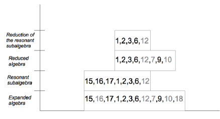
Figure 2: Expansions of $\mathfrak{sl}(2,\mathbb{R})$ with abelian semigroups of order $3$

For space reasons, only the label ‘$a$’ of the semigroup $S_{(3)}^{a}$ was written in the figure. The vertical axis illustrates the different types of expansions that can be performed and the boxes over the horizontal axis contain the semigroups that can be used for each case. The semigroups that preserve semisimplicity are labeled with a gray number and, as we can see, it might happen that a semigroup preserves semisimplicity in one level but not in other. This is the case of the semigroup $S_{(3)}^{16}$, appearing in the sample output above, which preserves semisimplicity for the expanded algebra but not for the resonant subalgebra.

The results of the programs 42-45 (which can also be found in the file Output_examples.zip available in [56]) are sumarized in the following table.

$$n=2$$

#

#pss

This table gives for each order the number of semigroups which allows to generate: S-expanded algebras $\mathcal{G}_{S}$, reduced algebras $\mathcal{G}_{S,\text{red}}$, resonant subalgebras $\mathcal{G}_{S,R}$ and reductions of the resonant subalgebras $\mathcal{G}_{S,R,\text{red}}$. The number of expansions preserving semisimplicity, denoted by #pss, is given for each case. Besides, as shown in Sections 5.2 and 5.3, a given semigroup might have more than one resonance and thus, for the cases with resonances, we also give the total number of resonances #r.

The fraction of semigroups preserving semisimplicity is very small and remarkably, as shown explicitly in Section 4.2 of Ref. [55], expansions performed with those semisgroups always contains the original algebra as a subalgebra. For example, the semigroups $S_{\left(n\right)}^{a}$ of order $n=3,4,5$ with a zero element and a resonant decomposition that preserve semisimplicity are:

$$S_{\left(3\right)}^{12},\ S_{\left(4\right)}^{88},\ S_{\left(5\right)}^{770},\ S_{\left(5\right)}^{779},\ S_{\left(5\right)}^{922},\ S_{\left(5\right)}^{968},\ S_{\left(5\right)}^{990},\ S_{\left(5\right)}^{991}\,.$$

For some of them it is possible to perform more than one reduction consecutively and thus, it can be shown that the semigroups $S_{\left(3\right)}^{12}$, $S_{\left(4\right)}^{88}$, $S_{\left(5\right)}^{779}$ and $S_{\left(5\right)}^{922}$ leads after the whole process to the trivial result $\mathfrak{sl}(2,\mathbb{R})$. Expansions with $S_{\left(5\right)}^{770}$, $S_{\left(5\right)}^{968}$, $S_{\left(5\right)}^{990}$ leads essentially to $\mathfrak{sl}(2,\mathbb{R})\oplus\mathfrak{sl}(2,\mathbb{R})$, as it can be shown by performing a suitable change of basis. Finally, the expansion the semigroup $S_{\left(5\right)}^{991}$ leads to $\mathfrak{su}\left(2,\mathbb{R}\right)\oplus\mathfrak{sl}\left(2,\mathbb{R}\right)$.

One of the motivations used in [55] to study S-expansions preserving semisimplicity was the possibility of establishing some relations between the classical simple Lie algebras $A_{n}$, $B_{n}$, $C_{n}$, $D_{n}$ and the special ones. The detailed analysis revealed that the expansions preserving semisimplicity generate only direct sums of simple algebras, always containing the original one as a subalgebra. This lead to the conjecture that there is no S-expansion procedure relating them (at least with the resonant conditions considered here). However, a general proof for this statement still remains as an open problem.

Finally, the programs 36-41 are examples to study the compactness property of S-expanded alegbras (with semigroups of order $n=2,3,4$), in terms of the eigenvalues of the semigroup metric and the expanded Killing-Cartan metric given respectively in Eqs. (23) and (26). Following the procedure described in the previous section, these programs can be extended in order to study the compactness of resonant subalgebras and reduced algebras.

6 Comments

Motivated by the growing number of applications that the S-expansion method have had recently, mainly in the construction of higher dimensional gravity theories and the understanding of their interrelations, we have developed a computational tool to automatize this procedure. It is given as a Java library which is composed by 11 classes (listed in Section 2.5 and described in Sections 3 and 4) whose methods allows:

• To perform basic operations with semigroups (check associativity and commutativity, find the zero element, resonances and isomorphisms),

• To represent arbitrary Lie algebras and semigroups in order to perform S-expansions with arbitrary semigroups.

Many examples has been provided in Section 5 to solve a considerable number of problems. They are presented such that any user, not necessarilly an expert in Java, can easily modify them to perform his own calculations.

An important input we have used in many of our algorithms is the lists of all the non isomorphic semigroups generated by the Fortran program gen.f given in Ref. [71]. Consequently, this is an input based in the results of many works related to the classification of semigroups (some of them, the most importants for our purposes, were cited in Section 2.4). As mentioned in Ref. [71], the program gen.f should be able to generate in principle the full lists up to order 8. However, in our case we got them only up to order 6, because for some reason the program stops when reaches the 835,927th of the 836,021 semigroups of order 7. That is why, when we need to have the list of all non-isomorphic semigroups of a give order, we resctrict our calculations up to order 6. However, with our library we can still perform calculations with semigroups of order higher than 6 (see e.g., the examples in Sections 5.1 and 5.4). The only issue is that we do not have the full list of non isomorphic tables for those higher orders.

Besides, as our library has an open licence GNU, we expect not only that these lists can be updated soon for semigroups up to order 8 but also that some of its methods can be improved and extended. For example, a superalgebra has usually a subspace structure $\mathcal{G}$ $=V_{0}\oplus V_{1}\oplus V_{2}$ given by

$$\left[V_{0},V_{0}\right] \subset V_{0}\ ,\ \ \left[V_{0},V_{1}\right]\subset V_{1}\ ,\ \ \left[V_{0},V_{2}\right]\subset V_{2}$$

$$\left[V_{1},V_{1}\right] \subset V_{0}\oplus V_{2}\ ,\ \ \left[V_{1},V_{2}\right]\subset V_{1}\ ,\ \ \left[V_{2},V_{2}\right]\subset V_{0}\oplus V_{2}$$

so, according with Ref. [15], in order to perform S-expansions of superalgebras one needs to consider resonant decompositions $S=S_{0}\cup S_{1}\cup S_{2}$ satisfying

$$S_{0}\times S_{0} \subset S_{0}\ ,\ \ S_{0}\times S_{1}\subset S_{1}\ ,\ \ S_{0}\times S_{2}\subset S_{2}$$

$$S_{1}\times S_{1} \subset S_{0}\cap S_{2}\ ,\ \ S_{1}\times S_{2}\subset S_{1}\ ,\ \ S_{2}\times S_{2}\subset S_{0}\cap S_{2}$$

Therefore, an extension of the method described in Section 3.4 for this kind of resonances would allow to perform S-expansions of superalgebras with all the machinery developed in this work. It would also be useful to extend the library to perform resonant reductions which, as briefly mentioned at the end of Section 2.2, are more general than the $0_{S}$-reduction process.

Interestingly, in Ref. [75] it has been recently proposed an analytic method to answer if two given Lie algebras can be S-related. They consider resonances in which an element, different than zero, is not allowed to be repeated in the subsets of the considered decomposition of the semigroup. As our methods are able to find all possible resonant decompositions (allowing non-zero elements to be repeated), a method selecting the decompositions with non-repeated elements may be implemented in such a way that our library can also be useful for this kind of problem, at least for the case $S=S_{0}\cup S_{1}$. We will provide those methods in Ref. [76] as a first extension of this library, together with an independent and complementary procedure that we developed in parallel, in order to answer whether two given Lie algebras can be S-related.

On the other hand, as mentioned in the introduction, in the early 60’s it was conjectured that all solvable Lie algebras could be obtained as a contraction of a semisimple Lie algebra of the same dimension (see, e.g., [17, 18]). Although in 2006 there were found some contra-examples that disproved this supposition [19] that problem has been revisited very recently in the context of the S-expansion [20]. Whether this method fixes the classification of solvable Lie algebras still remains an open problem, therefore we think that the computational tools developed in this work might be useful to work this out.

It is also worth to mention that the fact that the S-expansion reproduces all the WW contractions does not imply that the S-expansion covers all possible contractions. As noticed in [20] there exist contractions that cannnot be realized by a WW contraction (see e.g., Refs.[77, 78]) and that is why it is still unclear whether all contractions can be obtained from S-expansions. On the other hand, we do know that there exist S-expansions that are not equivalent to any contraction (an explicit example is given in [20]) and, in general, this is the case of S-expansions with semigroups that do not belong to the family $S_{E}^{\left(N\right)}$ and/or the case of expansions that lead to algebras of dimension bigger than the original one. Thus, the computational tool provided on this article might also be useful to answer if S-expansions exhaust or not all possible contractions.

From the theoretical-physics point of view, the S-expansion method has been used to show that Chern-Simons (CS) or Born Infeld (BI) type gravities constructed with the $S_{E}^{\left(N\right)}$ family lead, on a certain limit, to higher dimensional General Relativity. Thus, between the possible new applications, the techniques developed in this paper might help to analyze if it is possible to uncover and classify all the relations of this type (some results on this particular problem will be submitted soon [79]). Besides, an extension of the method to calculate resonant decompositions able to expand superalgebras might also be very useful in the context of supergravity (see e.g., [80, 81]). In particular, it might be analyzed whether is possible to obtain standard five-dimensional supergravity (see [82]) from a Chern-Simons supergravity based on a suitable expanded superalgebra.

Another application is related with the so called Pure Lovelock (PL) theory [83, 84, 85], which is a higher dimensional theory that has recently called the attention by the fact that their black hole solutions are asymptotically indistinguishable from the ones in general relativity. In Refs. [86, 87] an atempt to obtain PL gravity from CS and BI type gravities has been carried out using the expanded algebras. The relation is obtained at the level of the action, but present some problems at the level of the field equations, which can be fixed only by performing suitable identifications of the fields. Thus, the methods of this library could be used to look for a suitable S-expanded algebra giving the right dynamical limit and without performing identification of the fields (see [88]).

Apart from the mentioned applications in gravity theories and Lie group theory, it would be interesting analize if this tool could have also applications in other physical theories related with symmetries as well as in other branches, like semigroup theory and constraint logic programming. Besides, Lie algebras and semigroups has been recently applied in robotics and artificial intelligence so it would also be interesting to explore possible applications of this methods in this area too.

Appendix A List of program examples

In this Appedix we give the list of 45 example programs included in the file examples.zip available in [56]. Most of them has been described in Section 5 and, according to the classification explained in section 2.5, they are called generically as “prefix_name”.

1. I_associative_checking.java

2. I_commutative_checking.java

3. I_commutative_ord2_to_6.java

4. I_isomorphisms_ex1.java

5. I_isomorphisms_ex2.java

6. I_isomorphisms_ex3.java

7. I_isomorphisms_SE_N.java

8. I_Permutations_and_inverses_console_n4.java

9. I_Permutations_and_inverses_Order_2_to_7.java

10. I_PermuteWith_ex.java

11. II_AdjointRep_Casimirs_ex.java

12. II_Example_diagonalization.java

13. II_findAllResonances_console_ord4.java

14. II_findAllResonances_ord2_to_6.java

15. II_findresonances_ex_console.java

16. II_findresonances_ex.java

17. II_findzero_and_AllResonances_ord2_to_6.java

18. II_findzero_console_ord4.java

19. II_findzero_ex.java

20. II_findzero_ord2_to_6.java

21. II_isresonant_ex.java

22. II_isresonant_permute_ex1.java

23. II_isresonant_permute_ex2.java

24. II_isresonant_permute_ex3.java

25. II_isresonant_permute_ex4.java

26. II_S_and_G_AdjointRep_ex.java

27. II_SExp_CheckingByHand.java

28. II_SExp_sl2_S770.java

29. II_SExp_sl2_S968.java

30. II_SExp_sl2_S990.java

31. II_SExp_sl2_S991.java

32. II_SExpStructConst_sl2_S770.java

33. II_SExpStructConst_sl2_S968.java

34. II_SExpStructConst_sl2_S990.java

35. II_SExpStructConst_sl2_S991.java

36. III_EigenVectors_SExp_sl2_ord2.java

37. III_EigenVectors_SExp_sl2_ord3.java

38. III_EigenVectors_SExp_sl2_ord4.java

39. III_Signature_Sem_ord2.java

40. III_Signature_Sem_ord3.java

41. III_Signature_Sem_ord4.java

42. III_sl2_SExp_ord2_to_6_console.java

43. III_sl2_SExp_Red_ord2_to_6_console.java

44. III_sl2_SExp_Res_ord2_to_6_console.java

45. III_sl2_SExp_Res_Red_ord2_to_6_console.java

References

- [1] I.E. Segal, “A class of operator algebras which are determined by groups,” Duke Math. J 18(1951) 221
- [2] E. Inönü and E.P. Wigner, “On the contraction of groups and their representations,” Proc. Nat. Acad. Sci. U.S.A. 39, 510-524 (1953); E. Inönü, “Contractions of Lie groups and their representations,” in “Group theoretical concepts in elementary particle physics,” F. Gürseyed., Gordon and Breach, pp. 391-402 (1964)
- [3] E.J. Saletan, “Contractions of Lie groups,” J.Math. Phys. 2, 1-21 (1961).
- [4] M. Gerstenhaber, “On the deformations of rings and algebras,” Ann. Math. 79, 59-103 (1964)
- [5] A. Nijenhuis and R.W. Richardson Jr., “Cohomology and deformations in graded Lie algebras,” Bull. A, Math. Soc. 72, 1-29 (1966); A. Nijenhuis and R.W. Richardson Jr., Deformations of Lie algebra structures, J. Math. Mech. 171, 89-105 (1967)
- [6] R.W. Richardson, “On the rigidity of semi-direct products of Lie algebras,” Pac. J. Math. 22, 339-344 (1967)
- [7] Barut A. O. and Ratzka R. 1986 Theory of Group Representations and Applications (Singapore:World Scientific)
- [8] Gilmore R. 1974 Lie Groups, Lie Algebras, and Some of their Applications (New York: Wiley-Interscience)
- [9] E. Weimar-Woods, “Contractions of Lie algebras: generalized Inonu-Wigner contractions versus graded contractions,” J. Math. Phys. 36, 4519-4548 (1995); Jour. Math. Phys. 32 (1991) 2028; E. Weimar-Woods, “Contractions, generalized Inönü and Wigner contractions and deformations of finite-dimensional Lie algebras,” Rev. Math. Phys. 12, 1505-1529 (2000)
- [10] M. Hatsuda and M. Sakaguchi, “Wess-Zumino term for the AdS superstring and generalized Inonu-Wigner contraction,” Prog. Theor. Phys. 109 (2003) 853 [arXiv:hep-th/0106114].
- [11] J. A. de Azcarraga, J. M. Izquierdo, M. Picon and O. Varela, “Generating Lie and gauge free differential (super)algebras by expanding Maurer-Cartan forms and Chern-Simons supergravity,” Nucl. Phys. B 662 (2003) 185 [arXiv:hep-th/0212347].
- [12] J. A. de Azcarraga, J. M. Izquierdo, M. Picon and O. Varela, “Extensions, expansions, Lie algebra cohomology and enlarged superspaces,” Class. Quant. Grav. 21 (2004) S1375 [arXiv:hep-th/0401033].
- [13] J. A. de Azcarraga, J. M. Izquierdo, M. Picon and O. Varela, “Expansions of algebras and superalgebras and some applications,” Int. J. Theor. Phys. 46 (2007) 2738 [arXiv:hep-th/0703017].
- [14] M. Nakahara, Geometry, topology and physics, Institute of Physics publishing (1990).
- [15] F. Izaurieta, E. Rodriguez and P. Salgado, “Expanding Lie (super)algebras through Abelian semigroups,” J. Math. Phys. 47 (2006) 123512 [arXiv:hep-th/0606215].
- [16] J. Díaz, O. Fierro, F. Izaurieta, N. Merino, E. Rodríguez, P. Salgado and O. Valdivia, “A generalized action for (2 + 1)-dimensional Chern-Simons gravity,” J. Phys. A 45, 255207 (2012), [arXiv:1311.2215 [gr-qc]].
- [17] Zaitsev G.A., “Group-invariant study of the sets of limiting geometrie and special Lie subalgebras,” 1961, Talk thesises of All-USSR Geometric Conference (Kiev, USSR, 1961), 1-48 (Russian).
- [18] Celeghini E. and Tarlini M., “Contraction of group representations II,” Nuovo Cimento B 65 (1981), 172-180.
- [19] M. Nesterenko, R. Popovych, “Contractions of low-dimensional Lie algebras,” J. Math. Phys. 47 (2006) 123515.
- [20] Maryna Nesterenko, “S-expansions of three-dimensional Lie algebras,” Institute of Mathematics of NAS of Ukraine, 3 Tereshchenkivs’ka Str., Kyiv-4, 01601 Ukraine, arXiv:1212.1820; Maryna Nesterenko, “S-expansions of three-dimensional Lie algebras,” Group analysis of differential equations and integrable systems, 147-154, Department of Mathematics and Statistics, University of Cyprus, Nicosia, 2013.
- [21] J. Zanelli, “Lecture notes on Chern-Simons (super-)gravities. Second edition (February 2008),” hep-th/0502193.
- [22] F. Izaurieta, E. Rodriguez and P. Salgado, “Eleven-dimensional gauge theory for the M algebra as an Abelian semigroup expansion of osp(32—1),” Eur. Phys. J. C 54, 675 (2008), [hep-th/0606225].
- [23] F. Izaurieta, E. Rodriguez, A. Perez and P. Salgado, “Dual Formulation of the Lie Algebra S-expansion Procedure,” J. Math. Phys. 50 (2009) 073511 [arXiv:0903.4712 [hep-th]].
- [24] J. D. Edelstein, M. Hassaine, R. Troncoso and J. Zanelli, “Lie-algebra expansions, Chern-Simons theories and the Einstein-Hilbert Lagrangian,” Phys. Lett. B 640, 278 (2006) [hep-th/0605174].
- [25] F. Izaurieta, E. Rodriguez, P. Minning, P. Salgado and A. Perez, “Standard General Relativity from Chern-Simons Gravity,” Phys. Lett. B 678, 213 (2009) [arXiv:0905.2187 [hep-th]].
- [26] P. K. Concha, D. M. Peñafiel, E. K. Rodríguez and P. Salgado, “Even-dimensional General Relativity from Born-Infeld gravity,” Phys. Lett. B 725, 419 (2013) [arXiv:1309.0062 [hep-th]].
- [27] P. K. Concha, D. M. Peñafiel, E. K. Rodríguez and P. Salgado, “Chern-Simons and Born-Infeld gravity theories and Maxwell algebras type,” Eur. Phys. J. C 74, 2741 (2014) [arXiv:1402.0023 [hep-th]].
- [28] P. K. Concha, D. M. Peñafiel, E. K. Rodríguez and P. Salgado, “Generalized Poincaré algebras and Lovelock-Cartan gravity theory,” Phys. Lett. B 742, 310 (2015) [arXiv:1405.7078 [hep-th]].
- [29] S. Deser, G.W. Gibbons, “Born-Infeld-Einstein Actions?,” Class. Quant. Grav. 15 (1998) L35, [hep-th/9803049].
- [30] C. A. C. Quinzacara and P. Salgado, “Black hole for the Einstein-Chern-Simons gravity,” Phys. Rev. D 85, 124026 (2012) [arXiv:1401.1797 [gr-qc]].
- [31] C. A. C. Quinzacara and P. Salgado, “Stellar equilibrium in Einstein-Chern-Simons gravity,” Eur. Phys. J. C 73, no. 6, 2479 (2013).
- [32] J. Crisóstomo, F. Gómez, P. Salgado, C. Quinzacara, M. Cataldo and S. del Campo, “Accelerated FRW Solutions in Chern-Simons Gravity,” Eur. Phys. J. C 74, no. 10, 3087 (2014) [arXiv:1401.2128 [gr-qc]].
- [33] J. Crisóstomo, F. Gómez, C. Quinzacara and P. Salgado, “Static solutions in Einstein-Chern-Simons gravity,” arXiv:1601.06592 [gr-qc].
- [34] N. González, G. Rubio, P. Salgado and S. Salgado, “Generalized Galilean algebras and Newtonian gravity,” Phys. Lett. B 755, 433 (2016) [arXiv:1604.06313 [hep-th]].
- [35] R. Caroca, N. Merino and P. Salgado, “S-Expansion of Higher-Order Lie Algebras,” J. Math. Phys. 50, 013503 (2009) [arXiv:1004.5213 [math-ph]].
- [36] R. Caroca, N. Merino, A. Perez and P. Salgado, “Generating Higher-Order Lie Algebras by Expanding Maurer Cartan Forms,” J. Math. Phys. 50, 123527 (2009) [arXiv:1004.5503 [hep-th]].
- [37] R. Caroca, N. Merino, P. Salgado and O. Valdivia, “Generating infinite-dimensional algebras from loop algebras by expanding Maurer-Cartan forms,” J. Math. Phys. 52, 043519 (2011).
- [38] R. Caroca, I. Kondrashuk, N. Merino and F. Nadal, “Bianchi spaces and their three-dimensional isometries as S-expansions of two-dimensional isometries,” J. Phys. A 46, 225201 (2013) [arXiv:1104.3541 [math-ph]].
- [39] L. Bianchi, “Sugli spazi a tre dimensioni che ammettono un gruppo continuo di movimenti,” Memorie di Matematica e di Fisica della Societa Italiana delle Scienze, Serie Terza, Tomo XI, pp. 267–352 (1898).
- [40] D. V. Soroka and V. A. Soroka, “Semi-simple extension of the (super)Poincare algebra”, Adv. High Energy Phys. 2009, 234147 (2009), [hep-th/0605251].
- [41] R. Durka, J. Kowalski-Glikman and M. Szczachor, “Gauged AdS-Maxwell algebra and gravity,” Mod. Phys. Lett. A 26, 2689 (2011) [arXiv:1107.4728 [hep-th]].
- [42] R. Durka, J. Kowalski-Glikman and M. Szczachor, “AdS-Maxwell superalgebra and supergravity,” Mod. Phys. Lett. A 27, 1250023 (2012) [arXiv:1107.5731 [hep-th]].
- [43] P. Salgado and S. Salgado, “ algebras and gravity,” Phys. Lett. B 728, 5 (2014).
- [44] P. K. Concha, R. Durka, N. Merino and E. K. Rodríguez, “New family of Maxwell like algebras,” Phys. Lett. B 759, 507 (2016), [arXiv:1601.06443 [hep-th]].
- [45] P. Salgado, R. J. Szabo and O. Valdivia, “Topological gravity and transgression holography,” Phys. Rev. D 89, no. 8, 084077 (2014) [arXiv:1401.3653 [hep-th]].
- [46] O. Fierro, F. Izaurieta, P. Salgado and O. Valdivia, “(2+1)-dimensional supergravity invariant under the AdS-Lorentz superalgebra,” arXiv:1401.3697 [hep-th].
- [47] P. K. Concha and E. K. Rodríguez, “Maxwell Superalgebras and Abelian Semigroup Expansion,” Nucl. Phys. B 886, 1128 (2014), [arXiv:1405.1334 [hep-th]].
- [48] P. K. Concha and E. K. Rodríguez, “N = 1 Supergravity and Maxwell superalgebras,” JHEP 1409, 090 (2014), [arXiv:1407.4635 [hep-th]].
- [49] P. K. Concha, E. K. Rodríguez and P. Salgado, “Generalized supersymmetric cosmological term in Supergravity,” JHEP 1508, 009 (2015), [arXiv:1504.01898 [hep-th]].
- [50] P. K. Concha, O. Fierro, E. K. Rodríguez and P. Salgado, “Chern-Simons supergravity in and Maxwell superalgebra,” Phys. Lett. B 750, 117 (2015), [arXiv:1507.02335 [hep-th]].
- [51] M. C. Ipinza, P. K. Concha, L. Ravera and E. K. Rodríguez, “On the Supersymmetric Extension of Gauss-Bonnet like Gravity,” JHEP 1609, 007 (2016) [arXiv:1607.00373 [hep-th]].
- [52] P. K. Concha, O. Fierro and E. K. Rodríguez, “Inönü-Wigner Contraction and Supergravity,” arXiv:1611.05018 [hep-th].
- [53] R. Durka, “Resonant algebras and gravity,” arXiv:1605.00059 [hep-th].
- [54] D. M. Peñafiel and L. Ravera, “Generalized Inönü-Wigner Contraction as -Expansion with Infinite Semigroup and Ideal Subtraction,” arXiv:1611.05812 [hep-th].
- [55] L. Andrianopoli, N. Merino, F. Nadal and M. Trigiante, “General properties of the expansion methods of Lie algebras,” J. Phys. A 46, 365204 (2013) [arXiv:1308.4832 [gr-qc]].
- [56] https://github.com/SemigroupExp/Sexpansion/releases/tag/v1.0.0
- [57] R. Plemmons, “A survey of computer applications to semigroups and related structures,” ACM SIGSAM 12, (1969) 28-39.
- [58] F. Izaurieta, “Semigroup Expansion and M-Supergravity in Eleven Dimensions,” hep-th/0611238.
- [59] N. González, P. Salgado, G. Rubio and S. Salgado, “Einstein-Hilbert action with cosmological term from Chern-Simons gravity,” J. Geom. Phys. 86, 339 (2014).
- [60] G.E. Forsythe, “SWAC computes 126 distinct semigroups of order 4,” Proc. Amer. Math. Soc. 6, (1955) 443-447
- [61] T.S. Motzkin and J.L. Selfridge, “Semigroups of order five,” The November meeting in Los Angeles, Bull. Amer. Math. Soc. 62 (1) (1956) 13-23
- [62] R. Plemmons, “Construction and analysis of non-equivalent finite semigroups” (1970) Computational Problems in Abstract Algebra (Proc. Conf., Oxford, 1967) pp. 223-228 Pergamon, Oxford
- [63] R. Plemmons, “There are 15973 semigroups of order 6,” Math. Algorithms 2, (1967) 2-17
- [64] H. Jürgensen, P. Wick, “Die Halbgruppen der Ordnungen 7,” Semigroup Forum 14 (1977), 1, 69-79.
- [65] S. Satoh, K. Yama, M. Tokizawa, “Semigroups of order 8,” Semigroup Forum 49 (1994), 1, 7-29.
- [66] A. Distler, T. Kelsey, “The monoids of orders eight, nine & ten,” Ann. Math. Artif. Intell. 56 (2009), 3-21.
- [67] A. Distler and T. Kelsey, “The monoids of order eight and nine,” In S. Autexier, J. Campbell, J. Rubio, V. Sorge, M. Suzuki, and F. Wiedijk (Eds), Artificial Intelligence and Symbolic Computation, 8th International Conference, AISC 2008, Birmingham, July, 2008, Proceedings, volume 5144 of “Lecture Notes in Computer Science,” 61-76, Springer, 2008.
- [68] A. Distler and J.D. Mitchell, “Smallsemi - A library of small semigroups,” http://www-history.mcs.st-and.ac.uk/jamesm/smallsemi/, Feb 2010.
- [69] A. Distler, T. Kelsey and J.D. Mitchell, http://www-circa.mcs.st-and.ac.uk/
- [70] Andreas Distler, Chris Jefferson, Tom Kelsey and Lars Kotthof, “The Semigroups of Order 10,” Principles and Practice of Constraint Programming Volume 7514 of the series Lecture Notes in Computer Science pp 883-899, Springer Berlin Heidelberg. 18th International Conference, CP 2012, Québec City, QC, Canada, October 8-12, 2012. Proceedings. DOI 10.1007/978-3-642-33558-7_63
- [71] Hildebrant J 2001 Handbook of Finite Semigroup Programs (LSU Mathematics Electronic Preprint Series) preprint 2001-24
- [72] http://math.nist.gov/javanumerics/jama/
- [73] https://github.com/SemigroupExp/Sexpansion/wiki
- [74] M. Artebani, R. Caroca, M. C. Ipinza, D. M. Peñafiel and P. Salgado, “Geometrical aspects of the Lie algebra S-expansion procedure,” J. Math. Phys. 57, no. 2, 023516 (2016).
- [75] M. C. Ipinza, F. Lingua, D. M. Peñafiel and L. Ravera, “An Analytic Method for -Expansion involving Resonance and Reduction,” Fortsch. Phys. 64, no. 11-12, 854 (2016) [arXiv:1609.05042 [hep-th]].
- [76] C. Inostroza, I. Kondrashuk, N. Merino, F. Nadal, “Algorithm to find S-related Lie algebras,” Will be submitted soon.
- [77] D. Burde, “Degenerations of 7-dimensional nilpotent Lie algebras,” Comm. Algebra 33 (2005), 1259.
- [78] Popovych D.R. and Popovych R.O., “Lowest dimensional example on non-universality of generalized Inönü-Wigner contractions,” J. Algebra 324 (2010), 2742-2756.
- [79] P. K. Concha, C. Inostroza, N. Merino and E. K. Rodríguez, “Chern-Simons gravities related with General Relativity,” Will be submitted soon.
- [80] R. L. Arnowitt, P. Nath and B. Zumino, “Superfield Densities and Action Principle in Curved Superspace,” Phys. Lett. 56B, 81 (1975).
- [81] V. P. Akulov, D. V. Volkov and V. A. Soroka, “Gauge Fields on Superspaces with Different Holonomy Groups,” JETP Lett. 22, 187 (1975) [Pisma Zh. Eksp. Teor. Fiz. 22, 396 (1975)].
- [82] L. Castellani, R. D’Auria and P. Fre, Supergravity and Superstrings: A Geometric Perspective, World Scientific, Singapore, 1991.
- [83] R. G. Cai and N. Ohta, “Black Holes in Pure Lovelock Gravities,” Phys. Rev. D 74, 064001 (2006)
- [84] N. Dadhich, J. M. Pons and K. Prabhu, “On the static Lovelock black holes,” Gen. Rel. Grav. 45, 1131 (2013)
- [85] N. Dadhich, R. Durka, N. Merino and O. Miskovic, “Dynamical structure of Pure Lovelock gravity,” Phys. Rev. D 93, no. 6, 064009 (2016) [arXiv:1511.02541 [hep-th]].
- [86] P. K. Concha, R. Durka, C. Inostroza, N. Merino and E. K. Rodríguez, “Pure Lovelock gravity and Chern-Simons theory,” Phys. Rev. D 94, no. 2, 024055 (2016), [arXiv:1603.09424 [hep-th]].
- [87] P. K. Concha, N. Merino and E. K. Rodríguez, “Lovelock gravities from Born-Infeld gravity theory,” arXiv:1606.07083 [hep-th].
- [88] R. Durka, C. Inostroza and N. Merino, “Pure Lovelock gravity from Chern-Simons theory,” Work in progress.