Quantum Nonadiabatic Cloning of Entangled Coherent States

Abstract

We propose a systematic approach to the basis set extension for nonadiabatic dynamics of entangled combination of nuclear coherent states (CSs) evolving according to the time-dependent variational principle (TDVP). TDVP provides a rigorous framework for fully quantum nonadiabatic dynamics of closed systems, however, quality of results strongly depends on available basis functions. Starting with a single nuclear CS replicated vertically on all electronic states, our approach clones this function when replicas of the CS on different electronic states experience increasingly different forces. Created clones move away from each other (decohere) extending the basis set. To determine a moment for cloning we introduce generalized forces based on derivatives that maximally contribute to a variation of the total quantum action and thus account for entanglement of all basis functions.

The time-dependent variational principle (TDVP)Kramer and Saraceno (1981); Dirac (1958); Frenkel (1934) provides variationally optimal equations of motion (EOM) for the system wave-function specified by a certain ansatz. The TDVP allows one to model the quantum nuclear wave-function in a computationally efficient way for both adiabatic and nonadiabatic nuclear dynamics in molecules. There are two main popular forms of the nuclear wave-function: 1) originating from the multi-configuration time-dependent Hartree (MCTDH) methodMeyer, Manthe, and Cederbaum (1990); Wang and Thoss (2003a); G. A. Worth and Meyer and its multilayer generalizations,Wang and Thoss (2003b); Manthe (2008) 2) based on frozen-width gaussians, Yang et al. (2009); Ben-Nun and Martinez (2002); Shalashilin (2009); Burghardt, Giri, and Worth (2008); Worth, Robb, and Lasorne (2008); Worth, Robb, and Burghardt (2004); Izmaylov (2013); Makhov et al. (2014); Fernandez-Alberti et al. (2016) which are moving either classicallyYang et al. (2009); Ben-Nun and Martinez (2002); Shalashilin (2009); Makhov et al. (2014); Fernandez-Alberti et al. (2016) or quantum-mechanicallyBurghardt, Giri, and Worth (2008); Worth, Robb, and Lasorne (2008); Worth, Robb, and Burghardt (2004); Izmaylov (2013). The latter ansatz, due to locality of involved basis functions, is very well suited to be used in conjunction with the on-the-fly solution of the electronic structure problem. Ben-Nun and Martinez (2002); Shalashilin (2009); Fernandez-Alberti et al. (2016)

The main practical difficulty for any dynamical method based on the TDVP is basis set limitation. If we consider nonadiabatic dynamics using a linear combination of frozen-width gaussians

$$\ket{\Psi(t)}=\sum_{I=1}^{N_{G}}\sum_{s=1}^{N_{s}}C_{I}^{(s)}(t)\ket{G_{I}^{(s)}(t)}\ket{\phi_{s}},$$ (1)

where $C_{I}^{(s)}$ are time-dependent coefficients (amplitudes), indices $s$ and $I$ enumerate electronic states $\ket{\phi_{s}}$ and gaussians $\ket{G_{I}^{(s)}}$, respectively, the population transfer between electronic states can only take place when gaussians located on different electronic states have significant overlap in nuclear degrees of freedom (DOF), $\Braket{G_{I}^{(s)}\Big{}{}G_{J}^{(s^{\prime})}}{\gg}0$. However, considering localized nature of gaussians and that different electronic surfaces provide different forces in the same area of nuclear geometry, these overlaps generally quickly decay along the dynamics. This decoherence process artificially reduces the electronic population transfer. To address this issue, the spawning technique was introduced for a linear combination of frozen-width gaussians whose parameters evolved classically while the amplitudes were propagated quantum-mechanically.Yang et al. (2009); Ben-Nun and Martinez (2002) If a gaussian arrives at a region of strong coupling between electronic states and there is no gaussian on the other state to interact with it, the spawning algorithm creates the counterpart needed for population exchange (Fig. 1S). This consideration may seem ad hoc and does not account for the fact that each gaussian basis function is a part of the total nuclear wave-function. However, the spawning approach can be also rigorously introduced using time-dependent perturbation theoryIzmaylov (2013) that takes the total wave-function into account and provides a route for dynamical basis set extension. This perturbative spawning has been extended to the fully quantum propagation schemes such as the variational multiconfiguration gaussian (vMCG) method where gaussian dynamics has highly entangled quantum character.Izmaylov (2013)

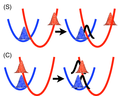
Figure 1: Illustration of the spawning (S) and cloning (C) procedures.

Alternatively, one can approach the problem of population transfer in TDVP based nonadiabatic dynamics by introducing a nuclear basis with the condition

$$\ket{G_{I}^{(s)}}=\ket{G_{I}^{(s^{\prime})}}=\ket{G_{I}},~{}s\neq s^{\prime}.$$ (2)

This condition will ensure the maximum overlap between gaussians on different electronic states $\Braket{G_{I}^{(s)}\Big{}{}G_{I}^{(s^{\prime})}}{=}1$. The wave-function becomes

$$\ket{\Psi(t)}=\sum_{I=1}^{N_{G}}\sum_{s=1}^{N_{s}}C_{I}^{(s)}(t)\ket{G_{I}(t)}\ket{\phi_{s}}$$ (3)

or equivalently

$$\ket{\Psi(t)}=\sum_{I=1}^{N_{G}}\ket{G_{I}(t)}\left[\sum_{s=1}^{N_{s}}C_{I}^{(s)}(t)\ket{\phi_{s}}\right].$$ (4)

Therefore, this basis, also known as the single-set (SS) basis, can be either thought as consisting of stacks of identical gaussians replicated for all electronic states [Eq. (3)] or gaussians with individual time-dependent electronic functions [Eq. (4)]. Although the SS gaussians always can exchange the population between electronic states, a new problem arises, replicas cannot take individual paths or decohere, instead each SS gaussian moves on an average, “Ehrenfest-like” surface. To introduce more freedom, the cloning technique was suggested,Makhov et al. (2014) the algorithm monitors difference in forces that replicas within an SS stack experience on different electronic states. When the force difference becomes large, the cloning scheme splits the stack of gaussians in two clones and adds empty replicas of gaussians for parts of the stack that went to another clone (Fig. 1C). As in the case of spawning, cloning has been introduced for frozen-width gaussians that are evolving classically on “Ehrenfest-like” surfaces.Makhov et al. (2014); Fernandez-Alberti et al. (2016) The algorithm treats every stack of gaussians independently, and thus, evaluation of forces is straightforward. However, such cloning has the same drawback as spawning: it does not treat each gaussian as a part of the total wave-function.

In order to put the cloning idea on a rigorous quantum basis as well as to extend it to fully quantum treatment of nuclear dynamics one should consider the case of quantum entangled gaussians with corresponding quantum forces that originate from the total nuclear wave-function. This is exactly the aim of the current Letter, where we propose a cloning algorithm for the fully quantum nonadiabatic dynamics in the basis of SS frozen-width gaussians.

For the sake of simplicity, our technique will be illustrated on a set of two-state low dimensional diabatic models where the exact quantum results can be easily obtained. However, nothing prevents the use of the approach in the adiabatic representation with the on-the-fly generation of potential electronic surfaces. To treat challenging geometric phase effects arising in the conical intersection caseMead and Truhlar (1979); Ryabinkin and Izmaylov (2013); Joubert-Doriol, Ryabinkin, and Izmaylov (2013); Ryabinkin, Joubert-Doriol, and Izmaylov (2014); Xie et al. (2016) one can use recently introduced scheme evaluating adiabatic electronic functions only at gaussian centres.Joubert-Doriol et al. (2017); Makhov et al. (2014); Fernandez-Alberti et al. (2016)

Equations of motion for the SS representation:

We start with the total non-stationary wave-function given by Eq. (4) where gaussians are taken in the coherent state (CS) form

$$\langle\mathbf{x}\ket{G_{I}(t)} = \prod_{j=1}^{N_{\rm dim}}\left(\frac{\omega_{j}}{\pi}\right)^{1/4}\exp\Big{[}-\frac{\omega_{j}}{2}[x_{j}-q_{jI}(t)]^{2}$$ (5)

$$+ip_{jI}[x_{j}-q_{jI}(t)]+\frac{i}{2}p_{jI}q_{jI}\Big{]}$$

here, $\mathbf{x}$ are nuclear coordinates, ${\rm dim}(\mathbf{x})=N_{\rm dim}$, and $\mathbf{q}_{I}(t)=\{q_{jI}(t)\}_{j=1,N_{\rm dim}}$ and $\mathbf{p}_{I}(t)=\{p_{jI}(t)\}_{j=1,N_{\rm dim}}$ are time-dependent positions and momenta. EOM for all parameters of the wave-function in Eq. (4) can be obtained by finding an extremum of the action $S=\int\bra{\Psi(t)}\hat{H}-i\partial_{t}\ket{\Psi(t)}dt$ which is equivalent to solvingBroeckhove et al. (1988)

$${\rm Re}\bra{\delta\Psi(t)}\hat{H}-i\partial_{t}\ket{\Psi(t)}=0.$$ (6)

Here, $\hat{H}$ is the system Hamiltonian. For the parametrization of Eq. (4) it is easy to show that such version of TDVP is equivalent to those of Dirac-FrenkelDirac (1958); Frenkel (1934) and McLachlanMcLachlan (1964). Introducing the SS variations

$$\ket{\delta\Psi}=\sum_{I,s}\Ket{\frac{\partial\Psi}{\partial C_{I}^{(s)}}}\delta C_{I}^{(s)}+\sum_{j,I}\Ket{\frac{\partial\Psi}{\partial q_{jI}}}\delta q_{jI}+\Ket{\frac{\partial\Psi}{\partial p_{jI}}}\delta p_{jI}$$ (7)

and accounting for independence and arbitrariness of individual variations $\delta C_{I}^{(s)}$, $\delta q_{jI}$, and $\delta p_{jI}$ leads to the EOM for all parametersWorth, Robb, and Lasorne (2008); Richings et al. (2015)

$$i\dot{C}_{I}^{(s)} = \sum_{J,s^{\prime}}\Big{[}\mathbf{S^{-1}}(\mathbf{H_{ss^{\prime}}}-i\boldsymbol{\tau}\delta_{ss^{\prime}})\Big{]}_{IJ}C_{J}^{(s^{\prime})},$$ (8)

$$i\dot{\xi}_{jI} = [\mathbf{B}^{-1}\mathbf{Y}]_{jI},$$ (9)

where $\xi_{jI}=\omega_{j}q_{jI}+ip_{jI}$ are convenient variables encoding both position and momentum components of CSs. Matrices involved in Eqs. (8) and (9) are

$$\tau_{IJ} = \bra{G_{I}}\partial_{t}G_{J}\rangle,~{}S_{IJ}=\bra{G_{I}}G_{J}\rangle,$$ (10)

$$H_{ss^{\prime},IJ} = \bra{G_{I}}\bra{\phi_{s}}\hat{H}\ket{\phi_{s^{\prime}}}\ket{G_{J}},$$ (11)

$$B_{Ik,Jn} = \sum_{s}C_{I}^{(s)*}C_{J}^{(s)}(\mathbf{S}^{(kn)}-\mathbf{S}^{(k0)}\mathbf{S}^{-1}\mathbf{S}^{(0n)})_{IJ}$$ (12)

$$Y_{Ik} = \sum_{ss^{\prime},J}C_{I}^{(s)*}C_{J}^{(s^{\prime})}(\mathbf{H}_{ss^{\prime}}^{(k0)}-\mathbf{S}^{(k0)}\mathbf{S}^{-1}\mathbf{H}_{ss^{\prime}})_{IJ},$$ (13)

$$H_{ss^{\prime},IJ}^{(k0)} = \Bra{\frac{\partial G_{I}}{\partial\xi_{kI}}}\bra{\phi_{s}}\hat{H}\ket{\phi_{s^{\prime}}}\Big{|}G_{J}\Big{\rangle},~{}S_{IJ}^{(kn)}=\Braket{\frac{\partial G_{I}}{\partial\xi_{kI}}\Big{}{}\frac{\partial G_{J}}{\partial\xi_{nJ}}}{,}~{}$$ (14)

$$S_{IJ}^{(k0)} = \Braket{\frac{\partial G_{I}}{\partial\xi_{kI}}\Big{}{}G_{J}}{,}~{}S_{IJ}^{(0n)}=\Braket{G_{I}\Big{}{}\frac{\partial G_{J}}{\partial\xi_{nJ}}}{.}$$ (15)

Time-derivatives of CSs needed in the $\boldsymbol{\tau}$ matrix are derived using the chain rule

$$\ket{\partial_{t}G_{K}} = \Ket{\frac{\partial G_{K}}{\partial\mathbf{q}_{K}}}\dot{\mathbf{q}}_{K}(t)+\Ket{\frac{\partial G_{K}}{\partial\mathbf{p}_{K}}}\dot{\mathbf{p}}_{K}(t).$$ (16)

Solving equations (8) and (9) constitutes the vMCG approach within the SS basis set.

Cloning SS pairs:

If we consider a variation of the total wave-function that changes positions and momenta of replicas for an $I^{th}$ CS on different electronic states independently

$$\ket{\delta_{I}\Psi}=\sum_{s,j}\Ket{\frac{\partial\Psi}{\partial\xi_{jI}^{(s)}}}\delta\xi_{jI}^{(s)},$$ (17)

the condition of Eq. (6) will not be satisfied. Formally, to consider such variation we need to evaluate it on a wave-function obtained from $\ket{\Psi}$ by allowing the $I^{th}$ CS’s replicas to be different for different electronic states

$$\ket{\Psi_{I}(t)}=\sum_{s}\left[C_{I}^{(s)}(t)\ket{G_{I}^{(s)}(t)}+\sum_{J\neq I}C_{J}^{(s)}(t)\ket{G_{J}(t)}\right]\ket{\phi_{s}}.$$ (18)

To determine when and which of the SS pairs to split for cloning, it is instructive to consider the variation

$${\rm Re}\bra{\delta_{I}\Psi_{I}}\hat{H}-i\partial_{t}\ket{\Psi_{I}} = {\rm Re}\left[\neq 0.$$ (19)

This quantity contains arbitrary variations $\delta\xi_{jI}^{(s)}$, which can be removed if one is interested in effect of splitting of the $I^{th}$ SS pair on the action. Thus, our criterion for splitting the $I^{th}$ SS pair is

$$\sum_{j,s}\left|>\varepsilon$$ (20)

where $\varepsilon$ is an accuracy threshold. Interestingly, since we use $\ket{\Psi_{I}}$ from the SS simulation, the sum of derivatives over electronic states is always zero,

$$\sum_{s}{\rm Re}\Braket{\frac{\partial\Psi_{I}}{\partial\xi_{jI}^{(s)}}\Bigg{}{}\hat{H}-i\partial_{t}\Bigg{}{}\Psi_{I}}{=}{0},$$ (21)

which is consistent with zero state average value. Therefore, the sum in Eq. (20) corresponds to the norm of the deviation of generalized quantum state specific forces acting on an individual CS from the state averaged counterpart.

Note, that more than one SS pair can be split using the criterion of Eq. (20) at a time, but for the sake of simplicity of further discussion we assume that only one pair has been split. Once the decision on splitting is made, to avoid linear dependency between clones, we propagate the split pair treated as independent CSs along with $N_{G}-1$ unsplit SS pairs. EOM for such hybrid evolution are obtained using TDVP applied to the parametrization $\Psi_{I}$ in Eq. (18) and detailed in the SI. CSs of the split pair move on different potential energy surfaces and necessarily decohere so that the overlap integral $\bra{G_{I}^{(1)}}G_{I}^{(2)}\rangle$ will decrease allowing to create two new SS pairs without introducing linear dependency

$$\begin{pmatrix}C_{I}^{(1)}\ket{G_{I}^{(1)}}\\ C_{I}^{(2)}\ket{G_{I}^{(2)}}\end{pmatrix}\rightarrow\begin{pmatrix}C_{I}^{(1)}\\ 0\end{pmatrix}\ket{G_{I}^{(1)}},~{}\begin{pmatrix}0\\ C_{I}^{(2)}\end{pmatrix}\ket{G_{I}^{(2)}}$$ (22)

where vectors are written in the basis of electronic functions $\{\phi_{s}\}_{s=1,2}$. Once the split CSs are cloned into two new SS pairs the regular EOM ((8) and (9)) for $N_{G}+1$ SS pairs are employed. We will refer to this algorithm as the quantum cloning vMCG (QC-vMCG) approach.

Numerical examples:

We illustrate the performance of QC-vMCG in modelling nuclear dynamics of one- and two-dimensional two-state diabatic models

$$\hat{H} = \sum_{j=1}^{N_{\rm dim}}\begin{pmatrix}[\hat{p}_{j}^{2}+\omega_{j}^{2}{x}_{j}^{2}]/2&c_{j}x_{j}\\ c_{j}x_{j}&[\hat{p}_{j}^{2}+\omega_{j}^{2}({x}_{j}-d_{j})^{2}]/2\end{pmatrix}+\begin{pmatrix}0&V\\ V&\Delta\end{pmatrix},$$ (23)

where $x_{j}$ and $\hat{p}_{j}$ are nuclear coordinates and associated momenta, and $V,~{}\Delta,~{}d_{j},~{}c_{j},~{}\omega_{j}$ are constants. In the one-dimensional (1D) model ($N_{\rm dim}=1$), which is also known as spin-boson, $\hat{H}_{\rm SB}=\hat{H}$ where $c_{j}=0$. In the two-dimensional (2D) model ($N_{\rm dim}=2$), $\hat{H}_{\rm CI}=\hat{H}$ where $V=d_{2}=c_{1}=0$, this setup gives rise to the conical intersection of potential energies if transformed to the adiabatic representation. Other parameters in both cases are $\omega_{1}=0.89$, $\omega_{2}=0.9$, $d_{1}=5$, and $\Delta=-\omega_{1}$. The last condition ensures resonance between vibrational levels of diabats coupled with linear potential coupling. Such resonances are unavoidable in large dimensional problems with conical intersections but can be missing in 2D models. We consider systems with strong and weak couplings, which are characterized by $V$ and $c_{2}$ for $\hat{H}_{\rm SB}$ and $\hat{H}_{\rm CI}$, respectively. Weak couplings simulate diabatically trapped systems,Izmaylov et al. (2011) while strong couplings bring systems closer to the adiabatic limit. However, strong nonadiabatic couplings are present in both cases. Also, large reorganization energy is maintained in all systems ($d_{1}=5$) to make them challenging for the SS basis. Note that $d_{j}=c_{j}=0$ case can be solved with a single SS pair because diabatic states have identical nuclear dependence in this limit.

We simulate nuclear dynamics starting with an initial wave-function constituting a single SS pair $\ket{\Psi(t=0)}=\ket{G_{1}}[1\cdot\ket{\phi_{1}}+0\cdot\ket{\phi_{2}}]$ with zero initial momentum and centred at point $\mathbf{q_{c}}$. For each Hamiltonian we simulate time-dependent wave-functions and monitor the population of the 1st electronic state, $P(t)={\rm Tr}_{n}[|\langle\phi_{1}\ket{\Psi(t)}|^{2}]$, where ${\rm Tr}_{n}$ is the trace over the nuclear coordinates (Fig. 2). In all QC-vMCG calculations lowering $\varepsilon$ allowed us to converge to the exact dynamics generated by the split operator approach.Tannor (2007) It may seem that lower couplings require lower thresholds, but it partly comes from the scale of the plots. Stronger couplings make initially empty replicas of CSs to be populated faster and to generate force difference for faster decoherence. Compare to 1D, in 2D there are more ways for CSs to avoid each other and to lower the overlap between different pairs. Mutual help of CSs is weaker in 2D, and thus, more CSs are required in 2D for convergence.

Besides cases in Fig. 2, decoherence forces of Eq. (20) for extreme limits of the spin-boson model have been considered: 1) $\hat{H}_{\rm SB}$ with $d_{1}=0$ produces zero derivatives in Eq. (20) because diabatic surfaces are parallel; 2) $\hat{H}_{\rm SB}$ with $V\rightarrow 0$ also produces zero derivatives in Eq. (20) because the population transfer is negligible, and the initial CSs evolves on a single harmonic oscillator. Also, in general case, it was confirmed that upon splitting not only derivatives in Eq. (20) of the split pair vanish but also derivatives of unsplit CSs are reduced. The latter is the effect that comes from quantum entanglement of CSs in the total nuclear wave-function.

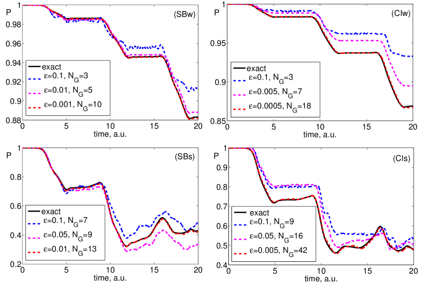
Figure 2: Electronic population as a function of time for $\hat{H}_{\rm SB}$ and $\hat{H}_{\rm CI}$ models for different couplings: (SBw) $\hat{H}_{\rm SB}$ weak coupling, $V=0.1\omega_{2}$; (SBs) $\hat{H}_{\rm SB}$ strong coupling, $V=0.5\omega_{2}$; (CIw) $\hat{H}_{\rm CI}$ weak coupling, $c_{2}=0.1\omega_{2}$; (CIs) $\hat{H}_{\rm CI}$ strong coupling, $c_{2}=0.5\omega_{2}$. In QC-vMCG (dashed curves) various $\varepsilon$’s produced different numbers of SS pairs at the end of the propagation, they are given by the $N_{G}$ values. Positions of the initial CS are $q_{c}=-3$ (1D) and $\mathbf{q_{c}}=(-3,-1)$ (2D).

In conclusion, we have introduced a novel general algorithm to extend basis set when needed in quantum dynamical simulations based on the magnitude of the quantum forces that have maximal effect on the action variation. These derivatives become large when pairs of nuclear CSs located on different potential energy surfaces are experiencing very different forces. Similar developments were done for classically moving CSs, where an ad hoc criteria of pair separation were introduced based on force differences. We rigorously extended these intuitive techniques to fully quantum dynamics of CSs, with account for entanglement between different CSs in the total wave-function. Our approach can be easily extended to more than two electronic states, the adiabatic representation, and on-the-fly generation of potential energy surfaces. Another useful extension can be a formulation of a spawning technique which will use similar derivatives to determine a spawning event variationally. The work on this approach is underway and will be reported elsewhere.

Acknowledgement: A.F.I. thanks I. G. Ryabinkin for critical reading of the manuscript and acknowledges funding from a Sloan Research Fellowship and the Natural Sciences and Engineering Research Council of Canada (NSERC) through the Discovery Grants Program.

References

- Kramer and Saraceno (1981) P. Kramer and M. Saraceno, Geometry of the Time-Dependent Variational Principle in Quantum Mechanics (Springer, New York, 1981).
- Dirac (1958) P. A. M. Dirac, The Principles of Quantum Mechanics, 4th Edition (Clarendon Press, Oxford, 1958).
- Frenkel (1934) J. Frenkel, Wave Mechanics (Clarendon Press, Oxford, 1934).
- Meyer, Manthe, and Cederbaum (1990) H.-D. Meyer, U. Manthe, and L. S. Cederbaum, Chem. Phys. Lett. 165, 73 (1990).
- Wang and Thoss (2003a) H. Wang and M. Thoss, J. Chem. Phys. 119, 1289 (2003a).
- (6) A. J. G. A. Worth, M. H. Beck and H.-D. Meyer, The MCTDH Package, Development Version 9.0, University of Heidelberg, Heidelberg, Germany, 2009.
- Wang and Thoss (2003b) H. Wang and M. Thoss, The Journal of Chemical Physics 119, 1289 (2003b).
- Manthe (2008) U. Manthe, The Journal of Chemical Physics 128, 164116 (2008).
- Yang et al. (2009) S. Yang, J. D. Coe, B. Kaduk, and T. J. Martínez, J. Chem. Phys. 130, 134113 (2009).
- Ben-Nun and Martinez (2002) M. Ben-Nun and T. J. Martinez, Adv. Chem. Phys. 121, 439 (2002).
- Shalashilin (2009) D. V. Shalashilin, J. Chem. Phys. 130, 244101 (2009).
- Burghardt, Giri, and Worth (2008) I. Burghardt, K. Giri, and G. A. Worth, J. Chem. Phys. 129, 174104 (2008).
- Worth, Robb, and Lasorne (2008) G. A. Worth, M. A. Robb, and B. Lasorne, Mol. Phys. 106, 2077 (2008).
- Worth, Robb, and Burghardt (2004) G. A. Worth, M. A. Robb, and I. Burghardt, Faraday Discuss. 127, 307 (2004).
- Izmaylov (2013) A. F. Izmaylov, J. Chem. Phys. 138, 104115 (2013).
- Makhov et al. (2014) D. V. Makhov, W. J. Glover, T. J. Martinez, and D. V. Shalashilin, J. Chem. Phys. 141, 054110 (2014).
- Fernandez-Alberti et al. (2016) S. Fernandez-Alberti, D. V. Makhov, S. Tretiak, and D. V. Shalashilin, Phys. Chem. Chem. Phys. 18, 10028 (2016).
- Mead and Truhlar (1979) C. A. Mead and D. G. Truhlar, J. Chem. Phys. 70, 2284 (1979).
- Ryabinkin and Izmaylov (2013) I. G. Ryabinkin and A. F. Izmaylov, Phys. Rev. Lett. 111, 220406 (2013).
- Joubert-Doriol, Ryabinkin, and Izmaylov (2013) L. Joubert-Doriol, I. G. Ryabinkin, and A. F. Izmaylov, J. Chem. Phys. 139, 234103 (2013).
- Ryabinkin, Joubert-Doriol, and Izmaylov (2014) I. G. Ryabinkin, L. Joubert-Doriol, and A. F. Izmaylov, J. Chem. Phys. 140, 214116 (2014).
- Xie et al. (2016) C. Xie, J. Ma, X. Zhu, D. R. Yarkony, D. Xie, and H. Guo, J. Am. Chem. Soc. 138, 7828 (2016).
- Joubert-Doriol et al. (2017) L. Joubert-Doriol, J. Sivasubramanium, I. G. Ryabinkin, and A. F. Izmaylov, The Journal of Physical Chemistry Letters , 452 (2017).
- Broeckhove et al. (1988) J. Broeckhove, L. Lathouwers, E. Kesteloot, and P. Van Leuven, Chemical Physics Letters 149, 547 (1988).
- McLachlan (1964) A. D. McLachlan, Molecular Physics 8, 39 (1964).
- Richings et al. (2015) G. W. Richings, I. Polyak, K. E. Spinlove, G. A. Worth, I. Burghardt, and B. Lasorne, International Reviews in Physical Chemistry , 161 (2015).
- Izmaylov et al. (2011) A. F. Izmaylov, D. Mendive Tapia, M. J. Bearpark, M. A. Robb, J. C. Tully, and M. J. Frisch, The Journal of Chemical Physics 135, 234106 (2011).
- Tannor (2007) D. J. Tannor, in Introduction to Quantum Mechanics: A Time-Dependent Perspective (University Science Books, Sausalito, California, 2007) p. 214.