Supersonic Flow onto Solid Wedges,
Multidimensional Shock Waves
and Free Boundary Problems

Abstract

When an upstream steady uniform supersonic flow impinges onto a symmetric straight-sided wedge, governed by the Euler equations, there are two possible steady oblique shock configurations if the wedge angle is less than the detachment angle – the steady weak shock with supersonic or subsonic downstream flow (determined by the wedge angle that is less or larger than the sonic angle) and the steady strong shock with subsonic downstream flow, both of which satisfy the entropy condition. The fundamental issue – whether one or both of the steady weak and strong shocks are physically admissible solutions – has been vigorously debated over the past eight decades. In this paper, we survey some recent developments on the stability analysis of the steady shock solutions in both the steady and dynamic regimes. For the static stability, we first show how the stability problem can be formulated as an initial-boundary value type problem and then reformulate it into a free boundary problem when the perturbation of both the upstream steady supersonic flow and the wedge boundary are suitably regular and small, and we finally present some recent results on the static stability of the steady supersonic and transonic shocks. For the dynamic stability for potential flow, we first show how the stability problem can be formulated as an initial-boundary value problem and then use the self-similarity of the problem to reduce it into a boundary value problem and further reformulate it into a free boundary problem, and we finally survey some recent developments in solving this free boundary problem for the existence of the Prandtl-Meyer configurations that tend to the steady weak supersonic or transonic oblique shock solutions as time goes to infinity. Some further developments and mathematical challenges in this direction are also discussed.

Primary: 35-02, 35M12, 35R35, 76H05, 76L05, 35L67, 35L65, 35B35, 35B30, 35B40, 35Q31, 76N10, 76N15, 35Q35, 35L60; Secondary: 35M10, 35B65, 35L70, 35L20, 35J70, 35B45, 35B36, 35B38, 35J67, 76J20, 76N20, 76G25

Citation:​​​​

CHEN Gui-Qiang. . Sci China Math, 2016, 59, doi:

1 Introduction

We survey some recent developments in the analysis of supersonic flow onto solid wedges (see Fig. 1.1), involving multidimensional shock waves, and related initial-boundary value type problems and free boundary problems for the Euler equations for compressible fluids. This paper is dedicated to Professor Tatsien on the occasion of his 80th birthday, who has made pioneering and fundamental contributions to this research direction and related areas (cf. [32, 41, 42, 43, 44, 45], [37, 38, 39], and the references cited therein), as we discussed below.

The wedge problem is a longstanding fundamental problem in mathematical fluid mechanics, partly owing to both the rich wave configurations in the fluid flow around the wedge and the mathematical challenges involved. More importantly, the solution configurations of the wedge problem are core configurations in the structure of global steady entropy solutions, as well as global dynamic entropy solutions of the two-dimensional Riemann problem, for multidimensional hyperbolic systems of conservation laws. The steady and Riemann solutions themselves are expected to be local building blocks and determine local structures, global attractors, and large-time asymptotic states of general entropy solutions for the systems. In this sense, we have to understand the solution configurations and their stability in order to understand fully the global entropy solutions of the multidimensional hyperbolic systems of conservation laws.

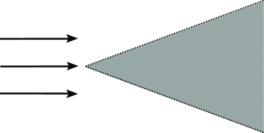
Figure 1.1: Upstream steady uniform supersonic flow past a symmetric straight-sided wedge

The two-dimensional steady, full Euler equations take the form:

$$\left\{\begin{aligned} &\nabla_{\mathbf{x}}\cdot(\rho\mathbf{u})=0,\\ &\nabla_{\mathbf{x}}\cdot\left(\rho{\mathbf{u}\otimes\mathbf{u}}\right)+\nabla_{\mathbf{x}}p=0,\\ &\nabla_{\mathbf{x}}\cdot\big{(}\rho\mathbf{u}(E+\frac{p}{\rho})\big{)}=0,\end{aligned}\right.$$ (1.1)

where $\nabla_{\mathbf{x}}$ is the gradient in $\mathbf{x}=(x_{1},x_{2})\in\mathbb{R}^{2}$, $\mathbf{u}=(u_{1},u_{2})$ the velocity, $\rho$ the density, $p$ the pressure, as well as

$$E=\frac{1}{2}|\mathbf{u}|^{2}+e$$ (1.2)

is the total energy with the internal energy $e$. The other two thermodynamic variables are temperature $T$ and entropy $S$. If $\rho$ and $S$ are chosen as the independent variables, then the constitutive relations can be written as

$$(e,p,T)=(e(\rho,S),p(\rho,S),T(\rho,S))$$

governed by $TdS=de-\frac{p}{\rho^{2}}d\rho.$ For an ideal gas,

$$p=R\rho T,\qquad e=c_{v}T,\qquad\gamma=1+\frac{R}{c_{v}}>1,$$ (1.3)

and

$$p=p(\rho,S)=\kappa\rho^{\gamma}{\rm e}^{S/c_{v}},\quad e=\frac{\kappa}{\gamma-1}\rho^{\gamma-1}{\rm e}^{S/c_{v}}=\frac{RT}{\gamma-1},$$ (1.4)

where $R,\kappa$, and $c_{v}$ are all positive constants.

The sonic speed of the polytropic gas flow is

$$c=\sqrt{\frac{\gamma p}{\rho}}.$$ (1.5)

The flow is subsonic if $|\mathbf{u}|<c$ and supersonic if $|\mathbf{u}|>c$. For a transonic flow, both cases occur in the flow, and then system (1.1) is of mixed-composite elliptic-hyperbolic type, which consists of two equations of mixed elliptic-hyperbolic type and two equations of transport-type (which are hyperbolic).

System (1.1) is a prototype of general nonlinear systems of conservation laws:

$$\nabla_{\mathbf{x}}\cdot\mathbf{F}(U)=0,\qquad\,\,\mathbf{x}\in\mathbb{R}^{n},$$ (1.6)

where $U:\mathbb{R}^{n}\to\mathbb{R}^{m}$ is unknown, while $\mathbf{F}:\mathbb{R}^{m}\to\mathbb{M}^{m\times n}$ is a given nonlinear mapping for the $m\times n$ matrix space $\mathbb{M}^{m\times n}$. For (1.1), we may choose $U=(\mathbf{u},p,\rho)$. The systems with form (1.6) often govern time-independent solutions of multidimensional quasilinear hyperbolic systems of conservation laws; cf. Dafermos [26] and Lax [40].

It is well known that, for an upstream steady uniform supersonic flow past a symmetric straight-sided wedge (see Fig. 1.1):

$$W:=\{\mathbf{x}=(x_{1},x_{2})\in\mathbb{R}^{2}\,:\,|x_{2}|<x_{1}\tan\theta_{\rm w},x_{1}>0\}$$ (1.7)

whose angle $\theta_{\rm w}$ is less than the detachment angle $\theta^{\rm d}_{\rm w}$, there exists an oblique shock emanating from the wedge vertex. Since the upper and lower subsonic regions do not interact with each other, it suffices to study the upper part. Then, more precisely, if the upstream steady flow is a uniform supersonic state, we can find the corresponding constant downstream flow along the straight-sided upper wedge boundary, together with a straight shock separating the two states. The downstream flow is determined by the shock polar whose states in the phase space are governed by the Rankine-Hugoniot conditions and the entropy condition; see Fig. 1.2 and §2. Indeed, Prandtl in [55] first employed the shock polar analysis to show that there are two possible steady oblique shock configurations when the wedge angle $\theta_{\rm w}$ is less than the detachment angle $\theta_{\rm w}^{\rm d}$ – The steady weak shock with supersonic or subsonic downstream flow (determined by the wedge angle that is less or larger than the sonic angle $\theta^{\rm s}_{\rm w}$) and the steady strong shock with subsonic downstream flow, both of which satisfy the entropy condition, provided that no additional conditions are assigned at downstream. See also Busemann [3], Courant-Friedrichs [25], Meyer [53], and the references cited therein.

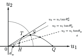
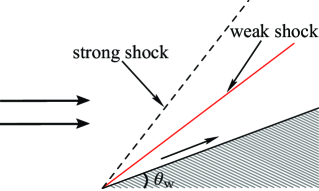
Figure 1.2: The shock polar in the $\mathbf{u}$-plane and uniform steady (weak and strong) shock flows

The fundamental issue – whether one or both of the steady weak and strong shocks are physically admissible – has been vigorously debated over the past eight decades (cf. [25, 26, 48, 54, 58]). On the basis of experimental and numerical evidence, it has strongly indicated that the steady weak shock solution would be physically admissible, as Prandtl conjectured in [55]. One natural approach to single out the physically admissible steady shock solutions is via the stability analysis: The stable ones are physical. For example, it is indicated in Courant-Friedrichs [25], Section 123, that “The question arises which of the two actually occurs. It has frequently been stated that the strong one is unstable and that, therefore, only the weak one could occur. A convincing proof of this instability has apparently never been given.” On August 17, 1949, during the Symposium on the Motion of Gaseous Masses of Cosmical Dimensions held at Paris, von Neumann [54] invited several eminent scientists of that days, including Burges, Heisenberg, Liepmann, von Kármán, and Temple, to join his discussion panel on the topic entitled “the Existence and Uniqueness of Multiplicity of Solutions of the Aerodynamical Equations”. In his open remarks, von Neumann made his comments specifically on the wedge problem: “Occasionally the simplest hydrodynamical problems have several solutions, some of which are very difficult to exclude on mathematical grounds only. For instance, a very simple hydrodynamical problem is that of the supersonic flow of a gas through a concave corner, which obviously leads to the appearance of shock wave. In general, there are two different solutions with shock waves, and it is perfectly well known from experimentation that only one of the two, the weaker shock wave, occurs in nature. But I think that all stability arguments to prove that it must be so, are of very dubious quality.” From these comments, one may see that von Neumann was not so optimistic then whether the mathematical stability analysis could provide a complete understanding of the non-uniqueness issue. After von Neumannn’s remarks, the panel members made their deep insights and different points of view for the admissibility of the weak and strong shock waves and related problems. For more details, we refer the reader to von Neumann [54]; see also [48, 58].

It is interesting to observe that there had not too much progress on the global stability analysis of the steady oblique shock solutions until recently; this is partly owing to the lack of mathematical tools and techniques that are required for solving the problem. Mathematically, there are two levels of the stability analysis of the multidimensional shock waves: One is the static stability of the shocks under steady perturbations within the steady regime, i.e., the steady perturbation of both the upstream supersonic flow and the wedge boundary; the other is the dynamic stability to show that the steady shock solutions are the long-time asymptotic limiting states of the corresponding unsteady solutions of the Euler equations for compressible fluids.

As far as we have known, the rigorous study of the local static stability of supersonic shock waves (i.e., both the upstream and downstream states are supersonic) around the wedge vertex for potential flow was first initiated by the Fudan Nonlinear PDE Group led by Chaohao Gu and Tatsien Li in 1960; see [32]. In this work, the shock wave involved was first regarded as a free boundary to formulate the stability problem as a free boundary problem, and was further reformulated the free boundary problem into a fixed boundary problem via the hodograph transform. The hodograph method was further refined by employing the parameterization method of characteristics in Gu-Li-Hou [37, 38, 39]. In [36], Gu extended the analysis of the wedge problem from the isentropic to full Euler equations and related quasilinear hyperbolic systems. In Li-Yu [43, 44] (see also [45]), a more general method of transformations was developed to analyze more general quasilinear hyperbolic systems. The local stability of the two-dimensional supersonic shock waves for the full Euler equations was proved in Li [41, 42] via employing the approach to solving free boundary problems for quasilinear hyperbolic systems, developed in Li-Yu [43, 44] (see also [45]), which considerably simplified the original proof of Schaeffer [56] that had been achieved via the Nash-Moser iterations. It is shown that the flow possesses the same qualitative features as a flow past a straight-sided wedge locally. The result in Li [41, 42] was obtained without the additional hypothesis of the Hölder continuity employed in [56] via the Nash-Moser iterations. See also Chen [16, 20] for the local static stability of supersonic shock waves past a three-dimensional wing and conical body for potential flow. For the first rigorous treatment of the local existence and stability of unsteady multidimensional shock fronts for nonlinear hyperbolic systems of conservation laws, see Majda [49, 50, 51]

The global stability results we present here are originally motivated by these fundamental results, insights, and remarks mentioned above. The purpose of this paper is to analyze the stability of both weak and strong shock waves, to show how the wedge problem can be formulated as mathematical problems – initial-boundary value type problems and free boundary problems, to present some recent developments, and to discuss further mathematical challenges and open problems in the global stability analysis of multidimensional shock waves.

More precisely, in Section 2, we first formulate the wedge problem as an initial-boundary value type problem, and then reformulate it into a free boundary problem. In Section 3, we present the global static stability of steady supersonic shocks under the BV perturbation of both the upstream steady supersonic flow and the slope of the wedge boundary, as long as the wedge vertex angle is less than the sonic angle. In Section 4, we present the global static stability of both weak and strong transonic shocks under the perturbation of both the upstream flow and the slope of the wedge boundary in a weighted Hölder space. In Section 5, we show that the steady weak supersonic/transonic shock solutions are the asymptotic limits of the dynamic self-similar solutions, the Prandtl-Meyer configurations. Finally, in Section 6, we discuss some further developments and mathematical challenges in this research direction.

2 Static Stability I: Mathematical Formulations and Free Boundary Problems

In this section, we first formulate the wedge problem as an initial-boundary value type problem, and then reformulate it into a free boundary problem when the perturbation of both the upstream steady supersonic flow and the wedge boundary are suitably regular and small.

In order that a piecewise smooth solution $U=(\mathbf{u},p,\rho)$ separated by a front $\mathcal{S}:=\{\mathbf{x}\,:\,x_{2}=\sigma(x_{1}),x_{1}\geq 0\}$ becomes a weak solution of the Euler equations (1.1), the Rankine-Hugoniot conditions must be satisfied along $\mathcal{S}$:

$$\begin{cases}\sigma^{\prime}(x_{1})[\,\rho u_{1}\,]=[\,\rho u_{2}\,],\\[2.84526pt] \sigma^{\prime}(x_{1})[\,\rho u_{1}^{2}+p\,]=[\,\rho u_{1}u_{2}\,],\\[2.84526pt] \sigma^{\prime}(x_{1})[\,\rho u_{1}u_{2}\,]=[\,\rho u_{2}^{2}+p\,],\\[2.84526pt] \sigma^{\prime}(x_{1})[\,\rho u_{1}(E+\frac{p}{\rho})\,]=[\,\rho u_{2}(E+\frac{p}{\rho})\,],\end{cases}$$ (2.1)

where $[\,\cdot\,]$ denotes the jump between the quantity of two states across front $\mathcal{S}$; that is, if $w^{-}$ and $w^{+}$ represent the left and right states, respectively, then $[w]:=w^{+}-w^{-}$.

Such a front $\mathcal{S}$ is called a shock if the entropy condition holds along $\mathcal{S}$: The density increases in the fluid direction across $\mathcal{S}$.

For given a state $U^{-}$, all states $U$ that can be connected with $U^{-}$ through the relations in (2.1) form a curve in the state space $\mathbb{R}^{4}$; the part of the curve whose states satisfy the entropy condition is called the shock polar. The projection of the shock polar onto the $\mathbf{u}$–plane is shown in Fig. 1.2.

In particular, for an upstream uniform horizontal flow $U_{0}^{-}=(u_{10}^{-},0,p_{0}^{-},\rho_{0}^{-})$ past the upper part of a straight-sided wedge whose angle is $\theta_{\rm w}$, the downstream constant flow can be determined by the shock polar (see Fig. 1.2). According to the shock polar, the two flow angles are important: One is the detachment angle $\theta_{\rm w}^{\rm d}$ that ensures the existence of an attached shock at the wedge vertex, and the other is the sonic angle $\theta_{\rm w}^{\rm s}<\theta_{\rm w}^{\rm d}$ for which the downstream fluid velocity is at the sonic speed in the direction. More precisely, in Fig. 1.2, $\theta_{\rm w}^{\rm s}$ is the wedge-angle such that line $u_{2}=u_{1}\tan\theta_{\rm w}^{\rm s}$ intersects with the shock polar at a point on the circle of radius $c_{0}$, and $\theta_{\rm w}^{\rm d}$ is the wedge-angle so that line $u_{2}=u_{1}\tan\theta_{\rm w}^{\rm d}$ is tangential to the shock polar and there is no intersection between line $u_{2}=u_{1}\tan\theta_{\rm w}$ and the shock polar when $\theta_{\rm w}>\theta_{\rm w}^{\rm d}$.

When the wedge angle is less than the detachment angle $\theta_{\rm w}^{\rm d}$, the tangent point $T$ corresponding to the detachment angle divides arc $\wideparen{HS}$ into the two open arcs $\wideparen{TS}$ and $\wideparen{TH}$; see Fig. 1.2. The nature of these two cases, as well as the case for arc $\wideparen{SQ}$, is very different. When the wedge angle $\theta_{\rm w}$ is between $\theta_{\rm w}^{\rm s}$ and $\theta_{\rm w}^{\rm d}$, there are two subsonic solutions; while the wedge angle $\theta_{\rm w}$ is smaller than $\theta_{\rm w}^{\rm s}$, there are one subsonic solution and one supersonic solution. Such an oblique shock $\mathcal{S}_{0}$ is also straight, described by $x_{2}=s_{0}x_{1}$. The question is whether the steady oblique shock solution is stable under a perturbation of both the upstream supersonic flow and the wedge boundary.

Assume that the perturbed upstream flow $U^{-}_{I}$ is close to $U_{0}^{-}$, which is supersonic and almost horizontal, and the wedge is close to a straight-sided wedge. Then, for any suitable wedge angle (smaller than a detachment angle), it is expected that there should be a shock attached to the wedge vertex. We now use a function $b(x_{1})\geq 0$ to describe the upper wedge boundary:

$$\partial\mathcal{W}=\{\mathbf{x}\in\mathbb{R}^{2}\,:\,x_{2}=b(x_{1}),\ b(0)=0\}.$$ (2.2)

Then the wedge problem can be formulated as the following problem:

Problem 2.1 (Initial-Boundary Value Type Problem).

Find a global solution of system (1.1) in $\Omega:=\{x_{2}>b(x_{1}),x_{1}>0\}$ such that the following holds:

1. Cauchy condition at $x_{1}=0$:

   $$U|_{x_{1}=0}=U^{-}_{I}(x_{2}){\rm;}$$ (2.3)

2. Boundary condition on $\partial\mathcal{W}$ as the slip boundary:

   $$\mathbf{u}\cdot\mathbf{n}|_{\partial\mathcal{W}}=0,$$ (2.4)

   where $\mathbf{n}$ is the outer unit normal vector to $\partial\mathcal{W}$.

Suppose that the background shock is the straight line given by $x_{2}=\sigma_{0}(x_{1})=s_{0}x_{1}$. When the upstream steady supersonic perturbation $U^{-}_{I}(x_{2})$ at $x_{1}=0$ is suitably regular and small, the upstream steady supersonic smooth solution $U^{-}(\mathbf{x})$ exists in region $\Omega^{-}=\Big{\{}\mathbf{x}\,:\,0<x_{1}<\frac{s_{0}}{2}x_{1}\Big{\}}$, beyond the background shock, but is still close to $U_{0}^{-}$.

Suppose that the shock wave $\mathcal{S}$ we seek is

$$\{\mathbf{x}\,:\,\sigma(0)=0,\,x_{2}=\sigma(x_{1}),x_{1}\geq 0\}.$$

The domain for the downstream flow behind $\mathcal{S}$ is denoted by

$$\Omega=\{\mathbf{x}\in\mathbb{R}^{2}\,:\,b(x_{1})<x_{2}<\sigma(x_{1}),x_{1}>0\}.$$ (2.5)

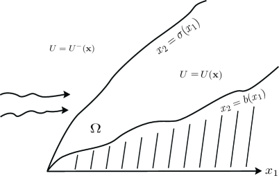
Figure 2.1: The leading steady shock as a free boundary under the perturbation

Then Problem 2.1 can be further reformulated into the following free boundary problem:

Problem 2.2 (Free Boundary Problem; see also Fig. 2.1).

Let $(U^{-}_{0},U^{+}_{0})$ be a constant transonic solution with transonic shock $\mathcal{S}_{0}:=\{x_{2}=\sigma_{0}(x_{1})=s_{0}x_{1}\}$. For any upstream flow $U^{-}$ for equations (1.1) in domain $\Omega^{-}$ as a small perturbation of $U^{-}_{0}$, find a shock $\mathcal{S}:=\{x_{2}=\sigma(x_{1})\}$ and a solution $U$ in $\Omega$ (see Fig. 2.1), which are small perturbations of $\mathcal{S}_{0}$ and $U^{+}_{0}$, respectively, such that

1. $U$ satisfies the equations in (1.1) in domain $\Omega$;

2. The slip condition (2.4) holds along the wedge boundary ${\partial}\mathcal{W}$;

3. The Rankine-Hugoniot conditions (2.1) as free boundary conditions hold along the shock front $\mathcal{S}$.

When $U^{+}_{0}$ corresponding to a state on arc $\wideparen{SQ}$ gives a weak supersonic shock (i.e., both the upstream and downstream states are supersonic) (see Fig. 1.2), the problem is denoted by Problem 2.2(SS); when $U^{+}_{0}$ corresponding to a subsonic state on arc $\wideparen{TS}$ gives a weak transonic shock (i.e., the upstream state is supersonic and the downstream state is subsonic) (see Fig. 1.2), the problem is denoted by Problem 2.2 (WT); while the strong transonic shock problem corresponds to arc $\wideparen{TH}$, denoted by Problem 2.2 (ST).

In general, the initial-boundary value type problem (Problem 2.1) is more general than the free boundary problem (Problem 2.2). On the other hand, the complete solution to the free boundary problem (Problem 2.2) provides the global structural stability of the steady oblique shocks, as well as more detailed structure of solutions.

3 Static Stability II: Steady Supersonic Shocks

If the downstream flow is supersonic (i.e., $U_{0}^{+}\in\wideparen{SQ}$), the corresponding shock is a weaker supersonic shock.

As indicated in §2, the rigorous study of the local static stability of such shock waves around the wedge vertex for the potential flow equation was first initiated by the Fudan Nonlinear PDE Group led by Gu and Li in [32]; also see [37, 38, 39, 36, 43, 44, 45]. For the full Euler equations, the local stability of the supersonic shocks was established by Gu [36], Li [41, 42], and Schaeffer [56] via different approaches.

Global potential solutions were constructed in [17, 18, 19, 24, 23, 60, 61] when the wedge has certain convexity or the wedge is a small perturbation of the straight-sided wedge with fast decay in the flow direction, whose vertex angle is less than the detachment angle. In particular, in Zhang [61], the existence of two-dimensional steady supersonic potential flows past piecewise smooth curved wedges, which are a small perturbation of the straight-sided wedge, was established.

For the free boundary problem Problem 2.2 (SS), the more general initial-boundary value type problem (Problem 2.1) has been solved for more general perturbations of both the initial data and wedge boundary, in Chen-Zhang-Zhu [14] and Chen-Li [13]. More precisely,

1. The wedge boundary function $x_{2}=b(x_{1})$ is a Lipschitz function, $b\in Lip(\mathbb{R}_{+})$, with

   $$TV(b^{\prime}(\cdot))<\infty,\quad b^{\prime}(0+)=0,\quad b(0)=0,\quad\arctan(b^{\prime}(x_{1}))<\theta_{\rm w}^{\rm s},$$

   so that ${\bf n}(x_{1}\pm)=\frac{(-b^{\prime}(x_{1}\pm),1)}{\sqrt{(b^{\prime}(x_{1}\pm))^{2}+1}}$ is the outer normal vector to $\Gamma$ at point $x\pm$ (see Fig. 3.1);

2. The upstream flow $U^{-}_{I}=(\mathbf{u}^{-}_{I},p^{-}_{I},\rho^{-}_{I})$ is a BV function (i.e., $U^{-}_{I}\in BV(\mathbb{R}_{+})$) satisfying that

   $$u^{-}_{I}>0,\qquad|\mathbf{u}^{-}_{I}|^{2}>(c^{-}_{I})^{2}:=\frac{\gamma p^{-}_{I}}{\rho^{-}_{I}}.$$

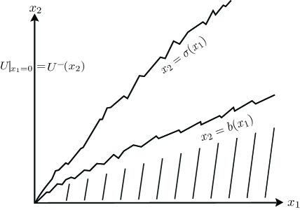
Figure 3.1: The leading supersonic shock as a Lipschitz free boundary under the BV perturbations

With this setup, we have

Theorem 3.1 (Chen-Zhang-Zhu [14] and Chen-Li [13]; see also Fig. 3.1).

There are $\varepsilon>0$ and $C>0$ such that, if

$$TV(U^{-}_{I}(\cdot))+TV(b^{\prime}(\cdot))<\varepsilon,$$ (3.1)

then there exists a pair of functions $(U(\mathbf{x}),\sigma(x_{1}))$:

$$U\in BV_{loc}(\mathbb{R}^{2}_{+}),\qquad\sigma^{\prime}\in BV(\mathbb{R}_{+}),$$

such that

(i) The curve, $x_{2}=\sigma(x_{1})$, is a leading shock above the wedge boundary $x_{2}=b(x_{1})$ for any $x_{1}>0$;

(ii) $U$ is a global entropy solution of Problem 2.1 in $\Omega:=\{\mathbf{x}\,:\,x_{2}>b_{1}(x_{1}),x_{1}\geq 0\}$ with

$$TV\{U(x_{1},\cdot)\,:\,(b(x_{1}),\sigma(x_{1}))\cup(\sigma(x_{1}),\infty)\}\leq C\big{(}TV(U^{-}_{I}(\cdot))+TV(b^{\prime}(\cdot))\big{)}\,\,\,\,\,\mbox{for any}\,\,x_{1}\in\mathbb{R}_{+},\qquad$$ (3.2)

$$(u,v)\cdot{\bf n}|_{x_{2}=b(x_{1})}=0\quad\mbox{in the trace sense};$$ (3.3)

(iii) There exist constants $s_{\infty}$ and $p_{\infty}$ such that

$$\lim_{x_{1}\rightarrow\infty}|\sigma^{\prime}(x_{1})-s_{\infty}|=0,\quad\lim_{x_{1}\rightarrow\infty}\sup\big{\{}|p(\mathbf{x})-p_{\infty}|\,:\;b(x_{1})<x_{2}<\sigma(x_{1})\big{\}}=0,$$

and

$$\lim_{x_{1}\rightarrow\infty}\sup\big{\{}\big{|}\frac{u_{2}(\mathbf{x})}{u_{1}(\mathbf{x})}-b^{\prime}(\infty)\big{|}\,:\;b(x_{1})<x_{2}<\sigma(x_{1})\big{\}}=0.$$

Moreover, the entropy solution $U=U(\mathbf{x})$ is stable with respect to the initial $BV$ perturbation in $L^{1}$ and unique in a broader class – the class of viscosity solutions.

This theorem indicates that the leading steady supersonic oblique shock-front emanating from the wedge vertex is nonlinearly stable in structure, although there may be many weaker waves and vortex sheets between the leading supersonic shock-front and the wedge boundary or the $x_{2}$–axis where the initial condition is assigned, under the $BV$ perturbation of both the upstream flow and the slope of the wedge boundary, as long as the wedge vertex angle is less than the sonic angle $\theta_{\rm w}^{\rm s}$. Moreover, the steady supersonic shock for the wedge problem is nonlinearly stable in $L^{1}$ under the $BV$ perturbation. This asserts that the steady supersonic oblique shock should be physical admissible, as observed from the experimental results.

More specifically, in Chen-Zhang-Zhu [14], in order to establish the global existence of solutions for the constant Cauchy data $U^{-}_{I}=U_{0}^{-}$, we first developed a modified Glimm scheme and identified a Glimm-type functional by incorporating the curved wedge boundary and the strong shock naturally, and by tracing the interactions not only between the wedge boundary and weak waves but also the interaction between the strong shock and weak waves. Some detailed interaction estimates are carefully made to ensure that the Glimm-type functional monotonically decreases in the flow direction. In particular, one of the essential estimates is on the strengths of the reflected waves for system (1.1) in the interaction between the strong shock and weak waves; and the second essential estimate is the interaction estimate between the wedge boundary and weak waves. Another essential estimate is on tracing the approximate strong shocks in order to establish the nonlinear stability and asymptotic behavior of the strong shock emanating from the wedge vertex under the wedge perturbation.

In Chen-Li [13], based on the understanding of the problem in Chen-Zhang-Zhu [14], we further established the $L^{1}$ well-posedness for Problem 2.1 when the total variation of both the boundary slope function and the Cauchy data (upstream flow) is small. We first obtained the existence of solutions in $BV$ when the upstream flow $U^{-}_{I}$ has small total variation by the wave front tracking method and then established the $L^{1}$–stability of the solutions with respect to the upstream flows. In particular, we incorporated the nonlinear waves generated from the wedge boundary to develop a Lyapunov functional between two solutions containing the strong shock fronts, which is equivalent to the $L^{1}$–norm, and proved that the functional decreases in the flow direction. Then the $L^{1}$–stability was established, which implies the uniqueness of the solutions by the wave front tracking method. Finally, the uniqueness of solutions in a broader class, the class of viscosity solutions, was also obtained.

4 Static Stability III: Weak and Strong Transonic Shocks

For transonic (i.e., supersonic-subsonic) shocks, there are two cases – the transonic shock with the subsonic state corresponding to arc $\wideparen{TS}$ (which is a weaker shock) and the one corresponding to arc $\wideparen{TH}$ (which is a stronger shock) (see Fig. 1.2). The strong shock case was first studied in Chen-Fang [23] for the potential flow. In Fang [31], the full Euler equations were studied with a uniform Bernoulli constant for both weak and strong transonic shocks. Because the framework is a weighted Sobolev space, the asymptotic behavior of the shock slope or subsonic solution was not derived. In Yin-Zhou [59], the Hölder norms were used for the estimates of solutions of the full Euler equations with the assumption on the sharpness of the wedge angle, which means that the subsonic state is near point $H$ in the shock polar. In Chen-Chen-Feldman [6], the weaker transonic shock, which corresponds to arc $\wideparen{TS}$, was investigated; and the existence, uniqueness, stability, and asymptotic behavior of subsonic solutions were obtained. In [6, 59], a potential function is used to reduce the full Euler equations to one elliptic equation in the subsonic region. The method was first proposed in [5] and has the advantage of integrating the conservation properties of the Euler system into a single elliptic equation. However, working on the potential function requires at least the Lipschitz estimate of the potential function to keep the subsonicity of the flow. In our recent paper [7], we have directly employed the decomposition of the full Euler equations into two algebraic equations and a first-order elliptic system of two equations and have established the stability and asymptotic behavior of transonic flows for Problem 2.2 (WT)–(ST) in a weighted Hölder space.

To state the results, following [7], we need to introduce the weighed Hölder norms in the subsonic domain $\Omega$, where $\Omega$ is either a truncated triangular domain or an unbounded domain with the vertex at origin ${O}$ and one side as the wedge boundary. There are two weights: One is the distance function to origin ${O}$ and the other is to the wedge boundary $\partial\mathcal{W}$. For any $\mathbf{x},\mathbf{x}^{\prime}\in\Omega$, define

$$\delta^{\rm o}_{\mathbf{x}}:=\min(|\mathbf{x}|,1),\quad\delta^{\rm o}_{\mathbf{x},\mathbf{x}^{\prime}}:=\min(\delta^{\rm o}_{\mathbf{x}},\delta^{\rm o}_{\mathbf{x}^{\prime}}),\quad\delta^{\rm w}_{\mathbf{x}}:=\min(\textrm{dist}(\mathbf{x},\partial\mathcal{W}),1),\quad\delta^{\rm w}_{\mathbf{x},\mathbf{x}^{\prime}}:=\min(\delta_{\mathbf{x}}^{\rm w},\delta_{\mathbf{x}^{\prime}}^{\rm w}),$$

$$\Delta_{\mathbf{x}}:=|\mathbf{x}|+1,\quad\Delta_{\mathbf{x},\mathbf{x}^{\prime}}:=\min(\Delta_{\mathbf{x}},\Delta_{\mathbf{x}^{\prime}}),\quad\widetilde{\Delta}_{\mathbf{x}}:=\textrm{dist}(\mathbf{x},\partial\mathcal{W})+1,\quad\widetilde{\Delta}_{\mathbf{x},\mathbf{x}^{\prime}}:=\min(\widetilde{\Delta}_{\mathbf{x}},\widetilde{\Delta}_{\mathbf{x}}).$$

Let $\alpha\in(0,1)$, $\tau,l,\gamma_{1},\gamma_{2}\in\mathbb{R}$ with $\gamma_{1}\geq\gamma_{2}$, and let $k$ be a nonnegative integer. Let $\mathbf{k}=(k_{1},k_{2})$ be an integer-valued vector, where $k_{1},k_{2}\geq 0$, $|\mathbf{k}|=k_{1}+k_{2}$, and $D^{\mathbf{k}}=\partial_{x_{1}}^{k_{1}}\partial_{x_{2}}^{k_{2}}$. We define

$$[f]_{k,0;(\tau,l);\Omega}^{(\gamma_{1};{O})(\gamma_{2};\partial\mathcal{W})}=\sup_{\begin{subarray}{c}\mathbf{x}\in\Omega\\ |\mathbf{k}|=k\end{subarray}}\begin{array}[]{l}\big{\{}(\delta^{\rm o}_{\mathbf{x}})^{\max\{\gamma_{1}+\min\{k,-\gamma_{2}\},0\}}(\delta^{\rm w}_{\mathbf{x}})^{\max\{k+\gamma_{2},0\}}\,\Delta_{\mathbf{x}}^{\tau}\widetilde{\Delta}_{\mathbf{x}}^{l+k}|D^{\mathbf{k}}f(\mathbf{x})|\big{\}},\end{array}$$ (4.2)

$${[f]}_{k,\alpha;(\tau,l);\Omega}^{(\gamma_{1};{O})(\gamma_{2};\partial\mathcal{W})}$$

$$\quad=\sup_{\begin{subarray}{c}\mathbf{x},\mathbf{x}^{\prime}\in\Omega\\ \mathbf{x}\neq\mathbf{x}^{\prime},|\mathbf{k}|=k\end{subarray}}\Big{\{}(\delta^{\rm o}_{\mathbf{x},\mathbf{x}^{\prime}})^{\max\{\gamma_{1}+\min\{k+\alpha,-\gamma_{2}\},0\}}(\delta^{\rm w}_{\mathbf{x},\mathbf{x}^{\prime}})^{\max\{k+\alpha+\gamma_{2},0\}}\Delta_{\mathbf{x},\mathbf{x}^{\prime}}^{\tau}\widetilde{\Delta}_{\mathbf{x},\mathbf{x}^{\prime}}^{l+k+\alpha}\frac{|D^{\mathbf{k}}f(\mathbf{x})-D^{\mathbf{k}}f(\mathbf{x}^{\prime})|}{|\mathbf{x}-\mathbf{x}^{\prime}|^{\alpha}}\Big{\}},$$ (4.3)

$$\|f\|_{k,\alpha;(\tau,l);\Omega}^{(\gamma_{1};{O})(\gamma_{2};\partial\mathcal{W})}=\sum_{i=0}^{k}{[f]}_{i,0;(\tau,l);\Omega}^{(\gamma_{1};{O})(\gamma_{2};\partial\mathcal{W})}+{[f]}_{k,\alpha;(\tau,l);\Omega}^{(\gamma_{1};{O})(\gamma_{2};\partial\mathcal{W})}.$$ (4.4)

For a vector-valued function $\mathbf{f}=(f_{1},f_{2},\cdots,f_{n})$, we define

$$\|\mathbf{f}\|_{k,\alpha;(\tau,l);\Omega}^{(\gamma_{1};{O})(\gamma_{2};\partial\mathcal{W})}=\sum_{i=1}^{n}\|f_{i}\|_{k,\alpha;(\tau,l);\Omega}^{(\gamma_{1};{O})(\gamma_{2};\partial\mathcal{W})}.$$

Let

$$C^{k,\alpha;(\tau,l)}_{(\gamma_{1};{O})(\gamma_{2};\partial\mathcal{W})}(\Omega)=\left\{f:\|f\|_{k,\alpha;(\tau,l);\Omega}^{(\gamma_{1};{O})(\gamma_{2};\partial\mathcal{W})}<\infty\right\}.$$ (4.5)

The requirement that $\gamma_{1}\geq\gamma_{2}$ in the definition above means that the regularity up to the wedge boundary is no worse than the regularity up to the wedge vertex. When $\gamma_{1}=\gamma_{2}$, the $\delta^{\rm o}$–terms disappear so that $(\gamma_{1},{O})$ can be dropped in the superscript. If there is no weight $(\gamma_{2},\partial\mathcal{W})$ in the superscript, the $\delta$–terms for the weights should be understood as $(\delta_{\mathbf{x}}^{\rm o})^{\max\{k+\gamma_{1},0\}}$ and $(\delta_{\mathbf{x}}^{\rm o})^{\max\{k+\alpha+\gamma_{1},0\}}$ in (4.2) and (4.3), respectively. Moreover, when no weight appears in the superscripts of the seminorms in (4.2) and (4.3), it means that neither $\delta^{\rm o}$ nor $\delta^{\rm w}$ is present. For a function of one variable defined on $(0,\infty)$, the weighted norm $\|f\|^{(\gamma_{2};0)}_{k,\alpha;(l);\mathbb{R}^{+}}$ is understood in the same as the definition above with the weight to $\{0\}$ and the decay at infinity.

Since the variables in $U$ are expected to have different levels of regularity, we distinguish these variables by defining ${U_{1}}=(u_{1},\rho)$ and $U_{2}=(w,p)$ for $w=\frac{u_{2}}{u_{1}}$. Let $U_{10}^{+}$ and $U_{20}^{+}$ be the corresponding background subsonic states.

Theorem 4.1 (Chen-Chen-Feldman [7]).

There are positive constants $\alpha,\beta,C_{0}$, and $\varepsilon$, depending only on the background states $(U^{-}_{0},U^{+}_{0})$, such that there exists a solution $(U,\sigma)$ for either of Problem 2.2 (WT) and Problem 2.2 (ST) such that $(U,\sigma)$ satisfies the following estimates:

1. For Problem 2.2 (WT),

   $$\begin{split}&\|U_{1}-U_{10}^{+}\|^{(-\alpha;{\partial}\mathcal{W})}_{2,\alpha;(0,1+\mathbf{\beta});\Omega}+\|U_{2}-U_{20}^{+}\|^{(-\alpha;{O})(-1-\alpha;{\partial}\mathcal{W})}_{2,\alpha;(1+\mathbf{\beta},0);\Omega}+\|\sigma^{\prime}-s_{0}\|^{(-\alpha;0)}_{2,\alpha;(1+\mathbf{\beta});\mathbb{R}^{+}}\\ &\leq{}C_{0}\left(\|U^{-}-U^{-}_{0}\|_{2,\alpha;(1+\beta,0);\Omega^{-}}+\|b^{\prime}\|^{(-\alpha;0)}_{1,\alpha;(1+\beta);\mathbb{R}^{+}}\right),\end{split}$$ (4.6)

   provided that

   $$\|U^{-}-U^{-}_{0}\|_{2,\alpha;(1+\beta,0);\Omega^{-}}+\|b^{\prime}\|^{(-\alpha;0)}_{1,\alpha;(1+\beta);\mathbb{R}^{+}}<\varepsilon;$$

2. For Problem 2.2 (ST),

   $$\begin{split}&\|U_{1}-U_{10}^{+}\|^{(-1-\alpha;\partial\mathcal{W})}_{2,\alpha;(0,\mathbf{\beta});\Omega}+\|U_{2}-U_{20}^{+}\|^{(-1-\alpha;{O})}_{2,\alpha;(\mathbf{\beta},0);\Omega}+\|\sigma^{\prime}-s_{0}\|^{(-1-\alpha;0)}_{2,\alpha;(\mathbf{\beta});\mathbb{R}^{+}}\\ &\leq{}C_{0}\left(\|U^{-}-U^{-}_{0}\|_{2,\alpha;(\beta);\Omega^{-}}+\|b^{\prime}\|^{(-1-\alpha;0)}_{2,\alpha;(\beta);\mathbb{R}^{+}}\right),\end{split}$$ (4.7)

   provided that

   $$\|U^{-}-U^{-}_{0}\|_{2,\alpha;(\beta,0);\Omega^{-}}+\|b^{\prime}\|^{(-\alpha-1;0)}_{2,\alpha;(\beta);\mathbb{R}^{+}}<\varepsilon.$$

The solution $(U,\sigma)$ is unique within the class of solutions such that the left-hand side of (4.6) for Problem 2.2 (WT) or (4.7) for Problem 2.2 (ST) is less than $C_{0}\varepsilon$.

The dependence of constants $\alpha,\beta,C_{0}$, and $\varepsilon$ in Theorem 4.1 is as follows: $\alpha$ and $\beta$ depend on $U^{-}_{0}$ and $U^{+}_{0}$, but are independent of $C_{0}$ and $\varepsilon$; $C_{0}$ depends on $U^{-}_{0},U^{+}_{0},\alpha$, and $b$, but are independent of $\varepsilon$; and $\varepsilon$ depends on all $U^{-}_{0},U^{+}_{0},\alpha,\beta$, and $C_{0}$.

The difference in the results of the two problems is that the solution of Problem 2.2 (WT) has less regularity at corner ${O}$ and decays faster with respect to $|\mathbf{x}|$ (or the distance from the wedge boundary) than the solution of Problem 2.2 (ST).

To achieve these, the main strategy is to use the physical variables to do the estimates, instead of the potential function. The advantage of this method is that only the lower regularity (i.e., the $C^{0}$–estimate) is enough to guarantee the subsonicity. Furthermore, directly estimating the physical state function $U$ also yields a better asymptotic decay rate: For weaker transonic shocks, in our earlier paper [6], the decay rate of the velocity is only $|\mathbf{x}|^{-\mathbf{\beta}}$; while, as indicated in (4.6) here, the subsonic solution decays to a limit state at rate $|\mathbf{x}|^{-\mathbf{\beta}-1}$.

More precisely, we have first used the Lagrangian coordinates to straighten the streamlines. The reason for this is that the Bernoulli variable and entropy are conserved along the streamlines. Using the streamline as one of the coordinates simplifies the formulation, especially for the asymptotic behavior of the solution. Then we have decomposed the Euler system into two algebraic equations and two elliptic equations, as in [22, 31]. Differentiating the two elliptic equations yields a second-order elliptic equation in divergence form for the flow direction $w=\frac{u_{2}}{u_{1}}$. Given $U$ for the coefficients in the equation, we can solve for a new variable $\tilde{w}$. Once we have solved for $\tilde{w}$ and obtained the desired estimates, the rest variables have then been updated so that a map $\delta\widetilde{U}=\mathcal{Q}(\delta U)$ has been constructed, where $\delta U$ and $\delta\widetilde{U}$ are the perturbations from the background subsonic state. The estimates based on our method do not yield the contraction for $\mathcal{Q}$. Therefore, the Schauder fixed point argument has been employed to obtain the existence of the subsonic solution. For the uniqueness, we have taken the difference of two solutions and have estimated the difference by using the weighted Hölder norms with less decay rate.

One point we should emphasize here is that the decay pattern is different from the potential flow. In a potential flow, the decay is with respect to $|\mathbf{x}|$. For example, if $\varphi$ converges to $\varphi_{0}$ at rate $|\mathbf{x}|^{-\mathbf{\beta}}$, then $\nabla\varphi$ converges at rate $|\mathbf{x}|^{-\mathbf{\beta}-1}$. For the Euler equations, because the Bernoulli variable and the entropy are constant along the streamlines, $U_{1}=(u_{1},\rho)$ does not converge to the background state along the streamlines, but does converge only across the streamlines away from the wedge. Therefore, when the elliptic estimates are performed, the scaling is with respect to the distance from the wedge, rather than $|\mathbf{x}|$. This results in the following decay pattern: In Lagrangian coordinates $\mathbf{y}$, there exists an asymptotic limit $U^{\infty}=(u_{1}^{\infty},0,p_{0}^{+},\rho^{\infty})$; $U$ converges to $U^{\infty}$ at rate $|\mathbf{y}|^{-\mathbf{\beta}}$, but $\nabla U$ converges at rate $|\mathbf{y}|^{-\mathbf{\beta}}(y_{2}+1)^{-1}$. That is, the extra decay for the gradient of the solution is only along the $y_{2}$–direction.

It would also be interesting to investigate the stability problems under more general perturbations, say the BV perturbation of both the upstream flow and the slope of the wedge boundary.

5 Dynamic Stability: Self-Similar Transonic Shocks and Existence of Prandtl-Meyer Configurations for Potential Flow

Since both weak and strong steady shock solutions are stable in the steady regime, the static stability analysis alone is not able to single out one of them in this sense, unless an additional condition is posed on the speed of the downstream flow at infinity. Then the dynamic stability analysis becomes more significant to understand the non-uniqueness issue of the steady oblique shock solutions. However, the problem for the dynamic stability of the steady shock solutions for supersonic flow past solid wedges involves several additional mathematical difficulties. The recent efforts have been focused on the construction of the global Prandtl-Meyer configurations in the self-similar coordinates for potential flow.

The compressible potential flow is governed by the conservation law of mass and the Bernoulli law:

$$\partial_{t}\rho+\nabla_{\bf x}\cdot(\rho\nabla_{\bf x}\Phi)=0,$$ (5.1)

$$\partial_{t}\Phi+\frac{1}{2}|\nabla_{\bf x}\Phi|^{2}+h(\rho)=B$$ (5.2)

for density $\rho$ and velocity-potential $\Phi$, where $B$ is the Bernoulli constant determined by the upstream flow and/or boundary conditions, and $h(\rho)$ is given by $h(\rho)=\int_{1}^{\rho}\frac{p^{\prime}(\varrho)}{\varrho}\,d\varrho=\int_{1}^{\rho}\frac{c^{2}(\varrho)}{\varrho}\,d\varrho$ for the sound speed $c(\rho)$ and pressure $p$. For an ideal polytropic gas, by scaling without loss of generality, the sound speed $c$ and pressure $p$ are given by

$$p(\rho)=\frac{\rho^{\gamma}}{\gamma},\qquad c^{2}(\rho)=\rho^{\gamma-1},\qquad h(\rho)=\frac{\rho^{\gamma-1}-1}{\gamma-1}$$ (5.3)

for the adiabatic component $\gamma>1$.

By (5.2)–(5.3), $\rho$ can be expressed as

$$\rho(\partial_{t}\Phi,\nabla_{\bf x}\Phi)=h^{-1}\bigl{(}B-\partial_{t}\Phi-\frac{1}{2}|\nabla_{\bf x}\Phi|^{2}\bigr{)}.$$ (5.4)

Then system (5.1)–(5.2) can be rewritten as

$$\partial_{t}\rho(\partial_{t}\Phi,\nabla_{\bf x}\Phi)+\nabla_{\bf x}\cdot\big{(}\rho(\partial_{t}\Phi,\nabla_{\bf x}\Phi)\nabla_{\bf x}\Phi\big{)}=0$$ (5.5)

with $\rho(\partial_{t}\Phi,\nabla_{\bf x}\Phi)$ determined by (5.4).

As we discussed earlier, if a supersonic flow with a constant density $\rho_{0}>0$ and a velocity ${\bf u}_{0}=(u_{10},0)$, $u_{10}>c_{0}:=c(\rho_{0})$, impinges toward wedge $W$ in (1.7), and if $\theta_{\rm w}$ is less than the detachment angle $\theta_{\rm w}^{\rm d}$, then the well-known shock polar analysis shows that there are two different steady weak solutions: the steady weak shock solution $\bar{\Phi}$ and the steady strong shock solution, both of which satisfy the entropy condition and the slip boundary condition (see Fig. 5.3).

Then the dynamic stability of the weak transonic shock solution for potential flow can be formulated as the following problem:

Problem 5.1 (Initial-Boundary Value Problem).

Given $\gamma>1$, fix $(\rho_{0},u_{10})$ with $u_{10}>c_{0}$. For a fixed $\theta_{\rm w}\in(0,\theta_{\rm w}^{\rm d})$, let $W$ be given by (1.7). Seek a global weak solution $\Phi\in W^{1,\infty}_{loc}(\mathbb{R}_{+}\times(\mathbb{R}^{2}\setminus W))$ of Eq. (5.5) with $\rho$ determined by (5.4) and $B=\frac{u_{10}^{2}}{2}+h(\rho_{0})$ so that $\Phi$ satisfies the initial condition at $t=0$:

$$(\rho,\Phi)|_{t=0}=(\rho_{0},u_{10}x_{1})\qquad\,\,\,\text{for}\;\;\mathbf{x}\in\mathbb{R}^{2}\setminus W,$$ (5.6)

and the slip boundary condition along the wedge boundary $\partial W$:

$$\nabla_{\bf x}\Phi\cdot{\bf n}_{\rm w}|_{\partial W}=0,$$ (5.7)

where ${\bf n}_{\rm w}$ is the exterior unit normal to $\partial W$.

In particular, we seek a solution $\Phi\in W^{1,\infty}_{loc}(\mathbb{R}_{+}\times(\mathbb{R}^{2}\setminus W))$ that converges to the steady weak oblique shock solution $\bar{\Phi}$ corresponding to the fixed parameters $(\rho_{0},u_{10},\gamma,\theta_{\rm w})$ with $\bar{\rho}=h^{-1}(B-\frac{1}{2}|\nabla\bar{\Phi}|^{2})$, when $t\to\infty$, in the following sense: For any $R>0$, $\Phi$ satisfies

$$\lim_{t\to\infty}\|(\nabla_{\bf x}\Phi(t,\cdot)-\nabla_{\bf x}\bar{\Phi},\rho(t,\cdot)-\bar{\rho})\|_{L^{1}(B_{R}({\bf 0})\setminus W)}=0$$ (5.8)

for $\rho(t,{\bf x})$ given by (5.4).

Since the initial data function in (5.6) does not satisfy the boundary condition (5.7), a boundary layer is generated along the wedge boundary starting at $t=0$, which forms the Prandtl-Meyer configuration, as proved in Bae-Chen-Feldman [1, 2].

Notice that the initial-boundary value problem, Problem 5.1, is invariant under the scaling:

$$(t,{\bf x})\rightarrow(\alpha t,\alpha{\bf x}),\quad(\rho,\Phi)\rightarrow(\rho,\frac{\Phi}{\alpha})\qquad\quad\text{for}\;\;\alpha\neq 0.$$

Thus, we seek self-similar solutions in the form of

$$\rho(t,{\bf x})=\rho({\bm{\xi}}),\quad\Phi(t,{\bf x})=t\phi({\bm{\xi}})\qquad\quad\text{for}\;\;{\bm{\xi}}=\frac{{\bf x}}{t}.$$

Then the pseudo-potential function $\varphi=\phi-\frac{1}{2}|{\bm{\xi}}|^{2}$ satisfies the following Euler equations for self-similar solutions:

$${\rm div}(\rho D\varphi)+2\rho=0,\qquad\frac{\rho^{\gamma-1}-1}{\gamma-1}+\big{(}\frac{1}{2}|D\varphi|^{2}+\varphi\big{)}=B,$$ (5.9)

where the divergence $div$ and gradient $D$ are with respect to ${\bm{\xi}}$. From this, we obtain the following equation for the pseudo-potential function $\varphi({\bm{\xi}})$:

$${\rm div}(\rho(|D\varphi|^{2},\varphi)D\varphi)+2\rho(|D\varphi|^{2},\varphi)=0$$ (5.10)

for

$$\rho(|D\varphi|^{2},\varphi)=\bigl{(}B_{0}-(\gamma-1)(\frac{1}{2}|D\varphi|^{2}+\varphi)\bigr{)}^{\frac{1}{\gamma-1}},$$ (5.11)

where we have set $B_{0}:=(\gamma-1)B+1$. Then we have

$$c^{2}(|D\varphi|^{2},\varphi)=B_{0}-(\gamma-1)\big{(}\frac{1}{2}|D\varphi|^{2}+\varphi\big{)}.$$ (5.12)

Equation (5.10) is an equation of mixed elliptic-hyperbolic type. It is elliptic if and only if

$$|D\varphi|<c(|D\varphi|^{2},\varphi).$$ (5.13)

As the upstream flow has the constant velocity $(u_{10},0)$, the corresponding pseudo-potential $\varphi_{0}$ has the expression of

$$\varphi_{0}=-\frac{1}{2}|{\bm{\xi}}|^{2}+u_{10}\xi_{1}.$$ (5.14)

Problem 5.1 can then be reformulated as the following boundary value problem in the domain:

$$\Lambda:=\mathbb{R}^{2}_{+}\setminus\{{\bm{\xi}}\,:\,\xi_{2}\leq\xi_{1}\tan\theta_{\rm w},\,\xi_{1}\geq 0\}$$

in the self-similar coordinates ${\bm{\xi}}$, which corresponds to domain $\{(t,{\bf x})\,:\,{\bf x}\in\mathbb{R}^{2}_{+}\setminus W,\,t>0\}$ in the $(t,{\bf x})$–coordinates.

Problem 5.2 (Boundary Value Problem).

Seek a solution $\varphi$ of equation (5.10) in the self-similar domain $\Lambda$ with the slip boundary condition:

$$D\varphi\cdot\mathbf{n}|_{\partial\Lambda}=0,$$ (5.15)

and the asymptotic boundary condition at infinity:

$$\varphi-\varphi_{0}\longrightarrow 0$$ (5.16)

along each ray $R_{\theta}:=\{\xi_{1}=\xi_{2}\cot\theta,\xi_{2}>0\}$ with $\theta\in(\theta_{\rm w},\pi)$ as $\xi_{2}\to\infty$ in the sense that

$$\lim_{r\to\infty}\|\varphi-\varphi_{0}\|_{C(R_{\theta}\setminus B_{r}(0))}=0.$$ (5.17)

In particular, we seek a weak solution of Problem 5.2 with two types of Prandtl-Meyer configurations whose occurrence is determined by the wedge angle $\theta_{\rm w}$ for the two different cases: One contains a straight weak oblique shock attached to the wedge vertex $O$, and the oblique shock is connected to a normal shock through a curved shock when $\theta_{\rm w}<\theta_{\rm w}^{\rm s}$, as shown in Fig. 5.1; the other contains a curved shock attached to the wedge vertex and connected to a normal shock when $\theta_{\rm w}^{\rm s}\leq\theta_{\rm w}<\theta_{\rm w}^{\rm d}$, as shown in Fig. 5.2, in which the curved shock $\Gamma_{\rm shock}$ is tangential to a straight weak oblique shock $S_{0}$ at the wedge vertex.

\psfrag{ls}[cc][0.8][0]{$\mathcal{S}_{0}$}\psfrag{sn}[cc][0.8][0]{$\mathcal{S}_{1}$}\psfrag{ol}[cc][0.8][0]{$\Omega_{1}$}\psfrag{on}[cc][0.8][0]{$\Omega_{2}$}\psfrag{lsn}[cc][0.8][0]{$\phantom{aa}\Gamma_{\rm sonic}^{1}$}\psfrag{rsn}[cc][0.8][0]{$\Gamma_{\rm sonic}^{2}\phantom{aaaaaaa}$}\psfrag{tw}[cc][0.8][0]{$\theta_{w}$}\psfrag{o}[cc][0.8][0]{$O$}\psfrag{lb}[cc][0.8][0]{$P_{4}$}\psfrag{rb}[cc][0.8][0]{$P_{3}$}\psfrag{lt}[cc][0.8][0]{$P_{1}$}\psfrag{rt}[cc][0.8][0]{$P_{2}$}\psfrag{s}[cc][0.8][0]{$\Gamma_{\rm shock}$}\psfrag{om}[cc][0.8][0]{$\Omega$}\includegraphics[scale={.5}]{prand3add.eps}

Figure 5.1: Self-similar solutions for $\theta_{\rm w}\in(0,\theta_{\rm w}^{\rm s})$ in the self-similar coordinates ${\bm{\xi}}$; see Bae-Chen-Feldman [1]

\psfrag{oi}[cc][0.8][0]{$\phantom{aaaaaaa}\Omega_{\infty}:(u_{10},0),\rho_{\infty}$}\psfrag{om}[cc][0.8][0]{$\Omega$}\psfrag{on}[cc][0.8][0]{$\Omega_{2}$}\psfrag{sn}[cc][0.8][0]{$\mathcal{S}_{1}$}\psfrag{ls}[cc][0.8][0]{$\mathcal{S}_{0}$}\psfrag{s}[cc][0.8][0]{\phantom{aaaaa}$\Gamma_{\rm shock}$}\psfrag{tw}[cc][0.8][0]{$\theta_{w}$}\includegraphics[scale={0.7}]{sol1.eps}

Figure 5.2: Self-similar solutions for $\theta_{\rm w}\in[\theta_{\rm w}^{\rm s},\theta_{\rm w}^{\rm d})$ in the self-similar coordinates ${\bm{\xi}}$; see Bae-Chen-Feldman [1]

A shock is a curve across which $D\varphi$ is discontinuous. If $\Omega^{+}$ and $\Omega^{-}(:=\Omega\setminus\overline{\Omega^{+}})$ are two nonempty open subsets of $\Omega\subset\mathbb{R}^{2}$, and $\mathcal{S}:=\partial\Omega^{+}\cap\Omega$ is a $C^{1}$-curve where $D\varphi$ has a jump, then $\varphi\in W^{1,1}_{loc}\cap C^{1}(\Omega^{\pm}\cup S)\cap C^{2}(\Omega^{\pm})$ is a global weak solution of (5.10) in $\Omega$ if and only if $\varphi$ is in $W^{1,\infty}_{loc}(\Omega)$ and satisfies equation (5.10) and the Rankine-Hugoniot condition on $\mathcal{S}$:

$$[\rho(|D\varphi|^{2},\varphi)D\varphi\cdot{\bm{\nu}}]_{\mathcal{S}}=0,$$ (5.18)

where $[F]_{\mathcal{S}}$ is defined by

$$[F({\bm{\xi}})]_{\mathcal{S}}:=F({\bm{\xi}})|_{\overline{\Omega^{-}}}-F({\bm{\xi}})|_{\overline{\Omega^{+}}}\qquad\quad\text{for}\;\;{\bm{\xi}}\in\mathcal{S}.$$

Note that the condition, $\varphi\in W^{1,\infty}_{loc}(\Omega)$, requires that

$$[\varphi]_{\mathcal{S}}=0.$$ (5.19)

The front, $\mathcal{S}$, is called a shock if density $\rho$ increases in the flow direction across $\mathcal{S}$. A piecewise smooth solution whose discontinuities are all shocks is called an entropy solution.

To seek a global entropy solution of Problem 5.2 with the structure of Fig. 5.1 or Fig. 5.2, one needs to compute the pseudo-potential function $\varphi_{0}$ below $S_{0}$.

Given $M_{0}>1$, $\rho_{1}$ and $\mathbf{u}_{1}$ are determined by using the shock polar in Fig. 5.3 for steady potential flow. For any wedge angle $\theta_{\rm w}\in(0,\theta_{\rm w}^{\rm s})$, line $u_{2}=u_{1}\tan\theta_{\rm w}$ and the shock polar intersect at a point $\mathbf{u}_{1}$ with $|\mathbf{u}_{1}|>c_{1}$ and $u_{11}<u_{10}$; while, for any wedge angle $\theta_{\rm w}\in[\theta_{\rm w}^{\rm s},\theta_{\rm w}^{\rm d})$, they intersect at a point $\mathbf{u}_{1}$ with $u_{11}>u_{\rm 1d}$ and $|\mathbf{u}_{1}|<c_{1}$. The intersection state $\mathbf{u}_{1}$ is the velocity for steady potential flow behind an oblique shock $\mathcal{S}_{0}$ attached to the wedge vertex with angle $\theta_{\rm w}$. The strength of shock $\mathcal{S}_{0}$ is relatively weak compared to the other shock given by the other intersection point on the shock polar, which is a weak oblique shock, and the corresponding state $\mathbf{u}_{1}$ is a weak state.

We also note that states $\mathbf{u}_{1}$ depend smoothly on $u_{10}$ and $\theta_{\rm w}$, and such states are supersonic when $\theta_{\rm w}\in(0,\theta_{\rm w}^{\rm s})$ and subsonic when $\theta_{\rm w}\in[\theta_{\rm w}^{s},\theta_{\rm w}^{\rm d})$.

\psfrag{tc}[cc][0.8][0]{$\phantom{aaaaaaaaaaa}u_{2}=u_{1}\tan\theta_{\rm w}^{\rm s}$}\psfrag{tw}[cc][0.8][0]{$\phantom{aaaaaaaaaaa}u_{2}=u_{1}\tan\theta_{w}$}\psfrag{td}[cc][0.8][0]{$\phantom{aaaaaaaaaaa}u_{2}=u_{1}\tan\theta_{\rm w}^{\rm d}$}\psfrag{u}[cc][0.8][0]{$u_{1}$}\psfrag{v}[cc][0.8][0]{$u_{2}$}\psfrag{u0}[cc][0.8][0]{$u_{10}$}\psfrag{zeta}[cc][0.8][0]{}\psfrag{ud}[cc][0.8][0]{$u_{\rm 1d}$}\includegraphics[scale={.8}]{shockpolar.eps}

Figure 5.3: The shock polar in the $\mathbf{u}$–plane

Once $\mathbf{u}_{1}$ is determined, by (5.14) and (5.19), the pseudo-potentials $\varphi_{1}$ and $\varphi_{2}$ below the weak oblique shock $\mathcal{S}_{0}$ and the normal shock $\mathcal{S}_{1}$ are respectively in the form of

$$\varphi_{1}=-\frac{1}{2}|{\bm{\xi}}|^{2}+\mathbf{u}_{1}\cdot{\bm{\xi}},\qquad\varphi_{2}=-\frac{1}{2}|{\bm{\xi}}|^{2}+\mathbf{u}_{2}\cdot{\bm{\xi}}+k_{2}$$ (5.20)

for constant states $\mathbf{u}_{1}$ and $\mathbf{u}_{2}$, and constant $k_{2}$. Then it follows from (5.11) and (5.20) that the corresponding densities $\rho_{1}$ and $\rho_{2}$ below $S_{0}$ and $S_{1}$ are constants, respectively. In particular, we have

$$\rho_{1}^{\gamma-1}=\rho_{0}^{\gamma-1}+\frac{\gamma-1}{2}\big{(}u_{10}^{2}-|\mathbf{u}_{1}|^{2}\big{)}.$$ (5.21)

Then Problem 5.2 can be reformulated into the following free boundary problem.

Problem 5.3 (Free Boundary Problem).

For $\theta_{\rm w}\in(0,\theta_{\rm w}^{\rm d})$, find a free boundary (curved shock) $\Gamma_{\rm shock}$ and a function $\varphi$ defined in domain $\Omega$, as shown in Figs. 5.1–5.2, such that $\varphi$ satisfies

• Equation (5.10) in $\Omega$;

• $\varphi=\varphi_{0}$ and $\rho D\varphi\cdot\mathbf{n}_{\rm s}=\rho_{0}D\varphi_{0}\cdot\mathbf{n}_{\rm s}$ on $\Gamma_{\rm shock}$;

• $\varphi=\hat{\varphi}$ and $D\varphi=D\hat{\varphi}$ on $\Gamma_{\rm sonic}^{1}\cup\Gamma_{\rm sonic}^{2}\,\,$ when $\theta_{\rm w}\in(0,\theta_{\rm w}^{s})$ and on $\Gamma_{\rm sonic}^{2}\cup\{O\}\,\,$ when $\theta_{\rm w}\in[\theta_{\rm w}^{\rm s},\theta_{\rm w}^{\rm d})$ for $\hat{\varphi}:=\max(\varphi_{1},\varphi_{2})$;

• $D\varphi\cdot\mathbf{n}=0$ on $\Gamma_{\rm wedge}$,

where $\mathbf{n}_{\rm s}$ and $\mathbf{n}$ are the interior unit normals to $\Omega$ on $\Gamma_{\rm shock}$ and $\Gamma_{\rm wedge}$, respectively.

Let $\varphi$ be a solution of Problem 5.3 such that $\Gamma_{\rm shock}$ is a $C^{1}$–curve up to its endpoints and $\varphi\in C^{1}(\overline{\Omega})$. To obtain a solution of Problem 5.2 from $\varphi$, we have two cases:

For $\theta_{\rm w}\in(0,\theta_{\rm w}^{\rm s})$, we divide the half-plane $\{\xi_{2}\geq 0\}$ into five separate regions. Let $\Omega_{\mathcal{S}}$ be the unbounded domain below curve $\overline{\mathcal{S}_{0}\cup\Gamma_{\rm shock}\cup\mathcal{S}_{1}}$ and above $\Gamma_{\rm wedge}$ (see Fig. 5.1). In $\Omega_{\mathcal{S}}$, let $\Omega_{1}$ be the bounded open domain enclosed by $\mathcal{S}_{0},\Gamma^{1}_{\rm sonic}$, and $\{\xi_{2}=0\}$. Set $\Omega_{2}:=\Omega_{S}\setminus\overline{(\Omega_{1}\cup\Omega)}$. Define a function $\varphi_{*}$ in $\{\xi_{2}\geq 0\}$ by

$$\varphi_{*}=\begin{cases}\varphi_{0}&\qquad\text{in}\,\Lambda\cap\{\xi_{2}\geq 0\}\setminus\Omega_{\mathcal{S}},\\ \varphi_{1}&\qquad\text{in}\,\Omega_{1},\\ \varphi&\qquad\text{in}\,\Gamma^{1}_{\rm sonic}\cup\Omega\cup\Gamma^{2}_{\rm sonic},\\ \varphi_{2}&\qquad\text{in}\,\Omega_{2}.\end{cases}$$ (5.22)

By (5.19) and (iii) of Problem 5.3, $\varphi_{*}$ is continuous in $\{\xi_{2}\geq 0\}\setminus\Omega_{S}$ and $C^{1}$ in $\overline{\Omega_{\mathcal{S}}}$. In particular, $\varphi_{*}$ is $C^{1}$ across $\Gamma^{1}_{\rm sonic}\cup\Gamma^{2}_{\rm sonic}$. Moreover, using (i)–(iii) of Problem 5.3, we obtain that $\varphi_{*}$ is a global entropy solution of equation (5.10) in $\Lambda\cap\{\xi_{2}>0\}$.

For $\theta_{w}\in[\theta_{\rm w}^{\rm s},\theta_{\rm w}^{\rm d})$, region $\Omega_{1}\cup\Gamma^{1}_{\rm sonic}$ in $\varphi_{*}$ reduces to one point $\{O\}$, and the corresponding $\varphi_{*}$ is a global entropy solution of equation (5.10) in $\Lambda\cap\{\xi_{2}>0\}$.

The first rigorous unsteady analysis of the steady supersonic weak shock solution as the long-time behavior of an unsteady flow is due to Elling-Liu [30], in which they succeeded in establishing a stability theorem for an important class of physical parameters determined by certain assumptions for the wedge angle $\theta_{\rm w}$ less than the sonic angle $\theta^{\rm s}_{\rm w}\in(0,\theta^{\rm d}_{\rm w})$ for potential flow.

Recently, in Bae-Chen-Feldman [1, 2], we have successfully remove the assumptions in Elling-Liu’s theorem [30] and established the stability theorem for the steady (supersonic or transonic) weak shock solutions as the long-time asymptotics of the global Prandtl-Meyer configurations for unsteady potential flow for all the admissible physical parameters even up to the detachment angle $\theta^{\rm d}_{\rm w}$ (beyond the sonic angle $\theta^{\rm s}_{\rm w}<\theta^{\rm d}_{\rm w}$). The global Prandtl-Meyer configurations involve two types of transonic transition – discontinuous and continuous hyperbolic-elliptic phase transitions for the fluid fields (transonic shocks and sonic circles). To establish this theorem, we have first solved the free boundary problem (Problem 5.3), involving transonic shocks, for all wedge angles $\theta_{\rm w}\in(0,\theta_{\rm w}^{\rm d})$ by employing the new techniques developed in Chen-Feldman [11] to obtain the monotonicity properties and uniform a priori estimates for admissible solutions. Therefore, we have achieved the existence of a self-similar weak solution with higher regularity to Problem 5.1 for all wedge angles $\theta_{\rm w}$ up to the detachment angle $\theta_{\rm w}^{\rm d}$.

More precisely, to solve this free boundary problem, we have followed the approach introduced in Chen-Feldman [11]. We have first defined a class of admissible solutions $\varphi$, which are the solutions of Prandtl-Meyer configuration, such that, when $\theta_{\rm w}\in(0,\theta_{\rm w}^{\rm s})$, equation (5.10) is strictly elliptic for $\varphi$ in $\overline{\Omega}\setminus(\Gamma_{\rm sonic}^{1}\cup\Gamma_{\rm sonic}^{2})$, $\max\{\varphi_{1},\varphi_{2}\}\leq\varphi\leq\varphi_{0}$ holds in $\Omega$, and the following monotonicity properties hold:

$$D(\varphi_{0}-\varphi)\cdot\mathbf{e}_{\mathcal{S}_{1}}\geq 0,\quad D(\varphi_{0}-\varphi)\cdot\mathbf{e}_{\mathcal{S}_{0}}\leq 0\qquad\quad\mbox{in $\Omega$},$$ (5.23)

where $\mathbf{e}_{\mathcal{S}_{0}}$ and $\mathbf{e}_{\mathcal{S}_{1}}$ are the unit tangential directions to lines $\mathcal{S}_{0}$ and $\mathcal{S}_{1}$, respectively, pointing to the positive $\xi_{1}$-direction. The monotonicity properties in (5.23) are the key to ensure that the shock is a Lipschitz graph in a cone of directions, so that the geometry of the problem is fixed, among other consequences. For $\theta_{\rm w}\in[\theta_{\rm w}^{\rm s},\theta_{\rm w}^{\rm d})$, admissible solutions have been defined similarly, with corresponding changes to the structure of subsonic reflection solutions.

Another key step for solving Problem 5.3 is to derive uniform a priori estimates for admissible solutions for any wedge angle $\theta_{\rm w}\in[0,\theta_{\rm w}^{\rm d}-\varepsilon]$ for each $\varepsilon>0$. In particular, for fixed $\gamma>1$, $u_{10}>0$, and $\varepsilon>0$, it has been proved that there exists a constant $C>0$ depending only on $\gamma,u_{10}$, and $\varepsilon>0$ such that, for any $\theta\in(0,\theta^{\rm d}_{\rm w}-\varepsilon]$, a corresponding admissible solution $\varphi$ satisfies

$${\rm dist}(\Gamma_{\rm shock},B_{c_{0}}(u_{10},0))\geq C^{-1}>0.$$

This inequality plays an essential role to achieve the ellipticity of equation (5.10) in $\Omega$. Once the ellipticity is achieved, then we can obtain various apriori estimates of $\varphi$, so that the Leray-Schauder degree argument can be employed to obtain the existence for each $\theta_{\rm w}\in[0,\theta_{\rm w}^{\rm d}-\varepsilon]$ in the class of admissible solutions, starting from the unique normal solution for $\theta_{\rm w}=0$. Since $\varepsilon>0$ is arbitrary, the existence of a weak solution for any $\theta_{\rm w}\in(0,\theta_{\rm w}^{\rm d})$ can be established.

More details can be found in Bae-Chen-Feldman [1, 2]; see also Chen-Feldman [11].

More recently, in Chen-Feldman-Xiang [12], we have also established the strict convexity of the curved transonic part of the free boundary in the Prandtl-Meyer configurations described above. In order to prove the convexity, we employ the global properties of admissible solutions, including the existence of the cone of monotonicity discussed above.

The existence results in Bae-Chen-Feldman [1, 2] indicate that the steady weak supersonic/transonic shock solutions are the asymptotic limits of the dynamic self-similar solutions, the Prandtl-Meyer configurations, in the sense of (5.17) in Problem 5.1.

On the other hand, it is shown in Elling [28] and Bae-Chen-Feldman [2] that, for each $\gamma>1$, there is no self-similar strong Prandtl-Meyer configuration for the unsteady potential flow in the class of admissible solutions (cf. [2]). This means that the situation for the dynamic stability of the strong steady oblique shocks is more sensitive.

6 Further Problems and Remarks

In §1–§5, we have surveyed some recent developments on the static stability of the weak and strong steady shock solutions for the wedge problem; we have also presented the recent results on the dynamic stability of the weak steady supersonic/transonic shock solutions for potential flow. These indicate that the weak supersonic/transonic oblique shocks are both stable, and it is more sensitive for the dynamic stability of the steady strong transonic shocks, which require further mathematical understanding. Moreover, there are many other open problems in this direction, which require further investigations.

When the deviation of vorticity become significant, the full Euler equations are required. It is still open how the Prandtl-Meyer configurations can be constructed for the full Euler flow. As seen in §5, we have understood the mathematical difficulties relatively well for the transonic shocks, the Kelydsh degeneracy near the sonic arcs, and the corner between the transonic shock and the sonic arcs for the nonlinear second-order elliptic equations, as well as a one-point singularity at the wedge vertex between the attached shock and the wedge boundary for the transition of state $(1)$ from the supersonic to subsonic states when the wedge angle increases across the sonic angle up to the detachment angle. On the other hand, when the flow is pseudo-subsonic, the system consists of two transport-type equations and two nonlinear equations of mixed hyperbolic-elliptic type. Therefore, in general, the full Euler system is of composite-mixed hyperbolic-elliptic type; see Chen-Feldman [11]. Then the following two new features for this problem for the isentropic and/or full Euler equations still need to be understood:

(i) Solutions of transport-type equations with rough coefficients and stationary transport velocity;

(ii) Estimates of the vorticity of the pseudo-velocity.

Indeed, a similar calculation as in Serre [57] has shown difficulties in estimating the vorticity. It is possible that the vorticity has some singularities in the region, perhaps near the wedge boundary and/or corner. In fact, even for potential flow, for the wedge angle $\theta_{\rm w}\in(\theta_{\rm w}^{\rm s},\theta_{\rm w}^{\rm d})$, the second derivatives of the velocity potential, i.e., the first derivatives of the velocity, may blow up at the wedge corner.

For the global stability of three or higher dimensional (M-D) transonic shocks in steady supersonic flow past M-D wedges, the situation is much more sensitive than that for the $2$-D case, which requires more careful rigorous mathematical analysis. In Chen-Fang [9], we developed a nonlinear approach and employed it to establish the stability of weak shock solutions containing a transonic shock for potential flow with respect to the M-D perturbation of the wedge boundary in appropriate function spaces. To achieve this, we first formulated the stability problem as an M-D free boundary problem for nonlinear elliptic equations. Then we introduced the partial hodograph transformation to reduce the free boundary problem into a fixed boundary value problem near a background solution with fully nonlinear boundary conditions for second-order nonlinear elliptic equations in an unbounded domain in M-D. To solve this reduced problem, we linearized the nonlinear problem on the background shock solution and then, after solving this linearized elliptic problem, we developed a nonlinear iteration scheme that was proved to be contractive, which implies the convergence of the scheme to yield the desired results. It would be interesting to investigate further problems for the stability of M-D shocks in steady supersonic flow past M-D wedges. In this regard, we notice that an instability result has been observed in Liang-Xu-Yin [46].

Conical flow (i.e., cylindrically symmetric flow with respect to an axis) occurs in many physical situations. For instance, it occurs at the conical nose of a projectile facing a supersonic stream of air (cf. [25]). The global stability of conical supersonic shocks has been studied in Liu-Lien [47] in the class of $BV$ solutions when the cone vertex angle is small, and Chen [21] and Chen-Xin-Yin [24] in the class of smooth solutions away from the conical shock when the perturbed cone is sufficiently close to the straight-sided cone. The stability of transonic shocks in 3-D steady flow past a perturbed cone had been a longstanding open problem. For the 2-D wedge case, the equations do not involve such singular terms, and the flow past the straight-sided wedge is piecewise constant. However, for the 3-D conical case, the governing equations have a singularity at the cone vertex and the flow past the straight-sided cone is self-similar, but no longer piecewise constant. These cause additional difficulties for the stability problem. In Chen-Fang [8], we developed techniques to handle the singular terms in the equations and the singularity of the solutions. Our main results indicate that the self-similar transonic shock is conditionally stable with respect to the conical perturbation of the cone boundary and the upstream flow in appropriate function spaces. That is, it was proved that the transonic shock and downstream flow in our solutions are close to the unperturbed self-similar transonic shock and downstream flow under the conical perturbation, and the slope of the shock asymptotically tends to the slope of the unperturbed self-similar shock at infinity. These results were obtained by first formulating the stability problem as a free boundary problem and introducing a coordinate transformation to reduce the free boundary problem into a fixed boundary value problem for a singular nonlinear elliptic system. Then we developed an iteration scheme that consists of two iteration mappings: One is for an iteration of approximate transonic shocks, and the other is for an iteration of the corresponding boundary value problems for the singular nonlinear systems for given approximate shocks. To ensure the well-definedness and contraction property of the iteration mappings, it is essential to establish the well-posedness for a corresponding singular linearized elliptic equation, especially the stability with respect to the coefficients of the equation, and to obtain the estimates of its solutions reflecting their singularity at the cone vertex and decay at infinity. The approach is to employ key features of the equation, to introduce appropriate solution spaces, and to apply a Fredholm-type theorem in Maz’ya-Plamenevskiǐ [52] to establish the existence of solutions by showing the uniqueness in the solution spaces.

Another important direction is to analyze the detached shocks off the wedge when the supersonic flow onto the wedge whose angle is larger than the detachment angle.

Finally, many fundamental problems in this direction are still wide open, and their solution requires further new techniques, approaches and ideas, which deserve our special attention.

The materials presented in this paper contain direct and indirect contributions of my collaborators Myoungjean Bae, Jun Chen, Beixiang Fang, Mikhail Feldman, Tianhong Li, Wei Xiang, Dianwen Zhu, and Yongqian Zhang. The work of Gui-Qiang G. Chen was supported in part by the US National Science Foundation under Grants DMS-0935967 and DMS-0807551, the UK Engineering and Physical Sciences Research Council under Grants EP/E035027/1 and EP/L015811/1, the National Natural Science Foundation of China (under joint project Grant 10728101), and the Royal Society–Wolfson Research Merit Award (UK).

References

- \bahao
- [1] Bae M J, Chen G -Q, Feldman M. Prandtl-Meyer reflection for supersonic flow past a solid ramp. Quart Appl Math, 2013, 71: 583–600
- [2] Bae M J, Chen G -Q, Feldman M. Prandtl-Meyer Reflection Configurations, Transonic Shocks and Free Boundary Problems. Research Monograpgh, Preprint, November 2016
- [3] Busemann A. Gasdynamik. Handbuch der Experimentalphysik, Vol. IV, Akademische Verlagsgesellschaft, Leipzig, 1931
- [4] Chang T, Hsiao L. The Riemann Problem and Interaction of Waves in Gas Dynamics. Longman Scientific & Technical, Harlow; copublished in the United States with John Wiley & Sons, Inc., New York, 1989
- [5] Chen G -Q, Chen J, Feldman M. Transonic shocks and free boundary problems for the full Euler equations in infinite nozzles. J Math Pures Appl (9), 2007, 88: 191–218
- [6] Chen G -Q, Chen J, Feldman M. Transonic flows with shocks past curved wedges for the full Euler equations. Discrete Conti Dyn Syst, 2016, 36: 4179–4211
- [7] Chen G -Q, Chen J, Feldman M. Stability and asymptotic behavior of transonic flows past wedges for the full Euler equations. Interfaces Free Boundaries, 2017, in press; arXiv: 1612.09538
- [8] Chen G-Q, Fang B. Stability of transonic shock-fronts in three-dimensional conical steady potential flow past a perturbed cone. Discrete Contin Dyn Syst, 2009, 23: 85–114
- [9] Chen G-Q, Fang B. Stability of transonic shocks in steady supersonic flow past multidimensional wedges. Adv Math, 2017, in press; arXiv:1603.03169
- [10] Chen G -Q, Feldman M. Multidimensional transonic shocks and free boundary problems for nonlinear equations of mixed type. J Amer Math Soc, 2003, 16: 461–494
- [11] Chen G -Q, Feldman M. The Mathematics of Shock Reflection-Diffraction and von Neumann’s Conjectures. Research Monograph, Princeton University Press, 2017
- [12] Chen G -Q, Feldman M, Xiang W. Convexity of self-similar transonic shock waves for potential flow. Preprint, December 2016
- [13] Chen G -Q, Li T -H. Well-posedness for two-dimensional steady supersonic Euler flows past a Lipschitz wedge. J Diff Eqs, 2008, 244: 1521–1550
- [14] Chen G -Q, Zhang Y -Q, Zhu D-W. Existence and stability of supersonic Euler flows past Lipschitz wedges. Arch Rational Mech Anal, 2006, 181: 261–310
- [15] Chen J, Christoforou C, Jegdić K. Existence and uniqueness analysis of a detached shock problem for the potential flow. Nonlinear Anal, 2011, 74: 705–720
- [16] Chen S -X. Existence of local solution to supersonic flow around a three-dimensional wing. Adv Appl Math, 1992, 13: 273–304
- [17] Chen S -X. Supersonic flow past a concave wedge. Science in China, 1997, 10A (27): 903–910
- [18] Chen S -X. Asymptotic behavior of supersonic flow past a convex combined wedge. Chin Ann Math, 1998, 19B: 255–264
- [19] Chen S -X. Global existence of supersonic flow past a curved convex wedge. J Partial Diff Eqs, 1998, 11: 73–82
- [20] Chen S -X. Existence of stationary supersonic flow past a pointed body. Arch Ration Mech Anal. 2001, 156: 141–181
- [21] Chen S -X. A free boundary problem of elliptic equation arising in supersonic flow past a conical body. Z Angew Math Phys. 2003, 54: 387–409
- [22] Chen S -X. Stability of transonic shock fronts in two-dimensional Euler system. Trans Amer Math Soc, 2005, 37: 287–308
- [23] Chen S -X, Fang B -X. Stability of transonic shocks in supersonic flow past a wedge. J Diff Eqs, 2007, 233: 105–135
- [24] Chen S -X, Xin Z, Yin H. Global shock waves for the supersonic flow past a perturbed cone. Commun Math Phys, 2002, 228: 47–84
- [25] Courant R, Friedrichs K O. Supersonic Flow and Shock Waves. New York: Wiley Interscience, 1948
- [26] Dafermos C M. Hyperbolic Conservation Laws in Continuum Physics. 4th Edition, Berlin: Springer-Verlag, 2016
- [27] Ding X -X, Chang T, Wang C -H, Hsiao L, Li T. -C. A study of the global solutions for quasilinear hyperbolic systems of conservation laws. Sci Sinica, 1973, 16: 317–335
- [28] Elling V. Non-existence of strong regular reflections in self-similar potential flow. J Diff Eqs, 2012, 252: 2085–2103
- [29] Elling V, Liu T -P. The ellipticity principle for self-similar potential flows. J Hyperbolic Diff Eqs, 2005, 2: 909–917
- [30] Elling V, Liu T -P. Supersonic flow onto a solid wedge. Comm Pure Appl Math, 2008, 61: 1347–1448
- [31] Fang B -X. Stability of transonic shocks for the full Euler system in supersonic flow past a wedge. Math Methods Appl Sci, 2006, 29: 1–26
- [32] Fudan Nonlinear PDE Group. On the problem of plane supersonic flow past a curved wedge. Page 17–28, In: Collection of Mathematical Papers, Department of Mathematics, Fudan University, Shanghai Science and Technology Press, 1960
- [33] Gilbarg D, Trudinger N. Elliptic Partial Differential Equations of Second Order. 2nd Ed. Berlin: Springer-Verlag, 1983
- [34] Glimm J. Solution in the large for nonlinear systems of conservation laws. Comm Pure Appl Math, 1965, 18: 695–715
- [35] Glimm J, Lax P D. Decay of Solutions of Systems of Hyperbolic Conservation Laws. Mem Amer Math Soc, 101, 1970
- [36] Gu C -H. A method for solving the supersonic flow past a curved wedge. Fudan J (Nature Sci), 1962, 7: 11–14
- [37] Gu C -H, Li T -T, Hou Z -Y. Discontinuous initial value problems for systems of quasi-linear hyperbolic equations. I. Acta Math Sinica, 1961, 11: 314–323 (Chinese); translated as Chinese Math, 1961, 2: 354–365
- [38] Gu C -H, Li T -T, Hou Z -Y. Discontinuous initial value problems for systems of quasi-linear hyperbolic equations. II. Acta Math Sinica, 1961, 11: 324–327 (Chinese); translated as Chinese Math, 1961, 2: 366–370
- [39] Gu C -H, Li T -T, Hou Z -Y. Discontinuous initial value problems for systems of quasi-linear hyperbolic equations. III. Acta Math Sinica, 1962, 12: 132–143 (Chinese); translated as Chinese Math, 1962, 3: 142–155
- [40] Lax P D. Hyperbolic Systems of Conservation Laws and the Mathematical Theory of Shock Waves. CBMS-RCSM, Philiadelphia: SIAM, 1973
- [41] Li T -T. Une remarque sur un problème à frontière libre. C R Acad Sci Paris Sér, 1979, A-B 289: A99–A102 (in French)
- [42] Li T -T. On a free boundary problem. Chinese Ann Math, 1980, 1: 351–358
- [43] Li T -T, Yu W -C. Some existence theorems for quasi-linear hyperbolic systems of partial differential equations in two independent variables. I. Typical boundary value problems. Sci Sinica, 1964, 13: 529–549
- [44] Li T -T, Yu W -C. Some existence theorems for quasi-linear hyperbolic systems of partial differential equations in two independent variables. II. Typical boundary value problems of functional formal and typical free boundary problems. Sci Sinica, 1964, 13: 551–562
- [45] Li T -T, Yu W -C. Boundary Value Problems for Quasilinear Hyperbolic Systems. Duke University Mathematics Series, 5. Duke University, Mathematics Department, Durham, NC, 1985
- [46] Li L, Xu G, Yin H. On the instability problem of a 3-D transonic oblique shock wave. Adv Math, 2015, 282: 443–515
- [47] Lien W, Liu T -P. Nonlinear stability of a self-similar 3-dimensional gas flow. Commun Math Phys, 1999, 204: 525–549
- [48] Liu T -P. Multi-dimensional gas flow: some historical perespectives. Bull Inst Math Acad Sinica (New Series), 2011, 6: 269–291
- [49] Majda A. The Stability of Multidimensional Shock Fronts. Mem Amer Math Soc, 41, no. 275, 1983
- [50] Majda A. The Existence of Multidimensional Shock Fronts. Mem Amer Math Soc, 43, no. 281, 1983
- [51] Majda A. Compressible Fluid Flow and Systems of Conservation Laws in Several Space Variables. Applied Mathematical Sciences, 53. Springer-Verlag: New York, 1984
- [52] Maz’ya V G, Plamenevskiǐ B A. Estimates in and in Hölder classes and the Miranda-Agman maximun principle for solutions of elliptic boundary value problems in domains with sigular points on the boundary. Amer Math Soc Transl, 1984, 123: 1–56
- [53] Meyer Th. Über zweidimensionale Bewegungsvorgänge in einem Gas, das mit Überschallgeschwindigkeit strömt. Dissertation, Göttingen, 1908. Forschungsheft des Vereins deutscher Ingenieure, Vol. 62, pp. 31–67, Berlin, 1908
- [54] von Neumann J. Discussion on the existence and uniqueness or multiplicity of solutions of the aerodynamical equations [Reprinted from MR0044302]. Bull Amer Math Soc (N.S.), 2010, 47: 145–154
- [55] Prandtl L. Allgemeine Überlegungen über die Strömung zusammendrückbarer Fluüssigkeiten. Zeitschrift für angewandte Mathematik und Mechanik, 1938, 16: 129–142
- [56] Schaeffer D G. Supersonic flow past a nearly straight wedge. Duke Math J, 1976, 43: 637–670
- [57] Serre D. Shock reflection in gas dynamics. In: Handbook of Mathematical Fluid Dynamics, Vol. 4, pp. 39–122, North-Holland: Elsevier, 2007
- [58] Serre D. von Neumann’s comments about existence and uniqueness for the initial-boundary value problem in gas dynamics. Bull Amer Math Soc (N.S.), 2010, 47: 139–144
- [59] Yin H, Zhou C. On global transonic shocks for the steady supersonic Euler flows past sharp 2-D wedges. J Diff Eqs, 2009, 246: 4466–4496
- [60] Zhang Y. Global existence of steady supersonic potential flow past a curved wedge with piecewise smooth boundary. SIAM J Math Anal, 1999, 31: 166–183
- [61] Zhang Y. Steady supersonic flow past an almost straight wedge with large vertex angle. J Diff Eqs, 2008, 192: 1–46