Determination of the strong coupling constant from ATLAS measurements of the inclusive isolated prompt photon cross section at $\sqrt{s}=7$ TeV.

Abstract

We present an estimation of the strong coupling constant $\alpha_{s}(M_{Z}^{2})$ using, for the first time, the production of prompt photon process in proton-proton collisions at the LHC. ATLAS measurements of the inclusive isolated prompt photon cross section at $\sqrt{s}=7$ TeV are exploited. Both theoretical and experimental uncertainties are estimated and the strong coupling constant has been determined to be $\alpha_{s}(M_{Z}^{2})=0.1183\pm 0.0038,$ to NLO accuracy.

I Introduction

The strong coupling "constant" $\alpha_{s}$ is the basic free parameter of Quantum Chromodynamics. QCD predicts that $\alpha_{s}(Q^{2})$ decreases with increasing energy or momentum transfer $Q$, and vanishes at asymptotically high energies. Testing the energy dependence (running) of $\alpha_{s}$ over a wide range provides an implicit test of QCD. Any modified running of the strong coupling may be a sign of new physics, for instance, a possible existence of new coloured matter near TeV energies is considered in Ref. new coloured matter .

$\alpha_{s}$ is not an “observable” by itself. Values of $\alpha_{s}(Q^{2})$ are determined from measurements of observables for which QCD predictions exist. Different particle reactions and scattering processes, performed at different energy scales $Q^{2}$, are used to extract the strong coupling parameter^[2]. In the theoretical framework, the Lattice QCD uses several approaches “which directly determine $\alpha_{s}$ on the lattice in a scheme closer to $\overline{\mathrm{MS}}$”^[3]; the ETM Collaboration uses a comparison of lattice data for the ghost-gluon coupling with that of perturbation theory^[4], providing the first determination of $\alpha_{s}$ with 2+1+1 flavors of dynamical quarks.

The energy reach available at the LHC makes possible, for the first time, to perform direct “measurements” of $\alpha_{s}(Q^{2})$ in the TeV scale. Jet production is used to extract $\alpha_{s}$ and to test its running with the momentum transfer up to the TeV region, currently to NLO accuracy^[5]and the CMS Collaboration reported the first determination of $\alpha_{s}$ using events from top-quark production, to NNLO accuracy^[6].

Here, we propose for the first time an extraction of the strong coupling constant using the prompt photon production process at the LHC. ATLAS measurements of the inclusive isolated cross section at $\sqrt{s}=7$ TeV is presented as a function of transverse energy $E_{T}^{\gamma}$ of the photon in the kinematic range $15\leq E_{T}^{\gamma}<1000$ GeV and the pseudo rapidity $\eta^{\gamma}$ regions $|\eta^{\gamma}|<1.37$ and $1.52\leq|\eta^{\gamma}|<2.37$^[7,8,9]. NLO calculations are performed using JETPHOX ^[10] with (NLO) CT10w parton density functions^[11], provided by the LHAPDF package${}^{[12]}.$

The paper is organized as follows. In Sec. II we present the theoretical predictions, involving the perturbative part and the non-pertubative corrections. Section III describes the extraction of the $\alpha_{s}$ from data and the averaging procedure. Both scale and PDF uncertainties are considered. The conclusion is presented in Sec. IV.

II The theoretical predictions

NLO differential cross-sections of isolated prompt photon production are calculated with the JETPHOX program^[10]. Further details on the scale and pdf uncertainties are available in papers note CERN ; note ATL , in region of phase space of interest.

The radius of the isolated cone is set to $R=0.4$ in $\eta-\varphi$ space around the photon direction and the maximum transverse energy cut deposited in the isolation cone (at the parton-level) is set to $(E_{T}^{\mathrm{iso}})_{max}=4\>\mathrm{and\>7\,GeV}$ as recommended in papers ATLAS1 and ATLAS3 respectively. Note that all ATLAS and CMS prompt photon measurements use the same definition of the cone isolation variable $E_{T}^{\mathrm{iso}}$ with a unique cone radius value $R=0.4$. This value seems to be the most suitable for the analysis.

The theoretical prediction are multiplied by an additional correction factor $C_{\mathrm{np}}$ to account for the presence of contributions from the underlying event and hadronization, using the Monte Carlo generator PYTHIA^[15].

The renormalization $\mu_{R}$, factorization $\mu_{F}$ and fragmentation $\mu_{f}$ scales are set to be equal:

$$\mu_{R}=\mu_{F}=\mu_{f}=\mu=E_{T}^{\gamma},$$ (II.1)

and the scale effects are evaluated using the uncertainty band varying the scales coherently and independently, (see Sec. III).

NLO calculations

The knowledge of the $\left(d\sigma/dE_{T}^{{}^{\gamma}}\right)_{\mathrm{NLO}}$ as functions of $\alpha_{s}(M_{Z}^{2})$ in each $(|\eta^{\gamma}|\mathrm{\mathrm{-}}E_{T}^{\gamma})$ bin is allowed using CT10wnlo_as_xxxx parametrizations presented for sixteen $\alpha_{s}(M_{Z}^{2})$ values in the range $0.112\mathrm{-}0.127$ in steps of $0.001$.

(a) $|\eta^{\gamma}|<0.6$

(b) $0.6<|\eta^{\gamma}|<1.37$

(c) $1.52<|\eta^{\gamma}|<1.81$

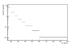
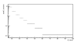
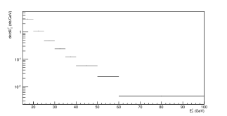
Figure II.1: NLO differential cross-sections multiplied by the non-prturbative coefficient $C_{\mathrm{np}}$, (CT10wnlo_as_0118, $E_{\mathrm{iso}}<4$ GeV)

The choice of this CTEQ set is motivated by its fine alphas scan and by the fact that it is largely used in theoretical calculations with consistent results in comparisons with data.

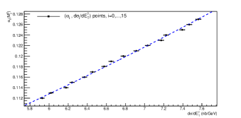
JETPHOX calculations are done for each pdf member (i.e. for each value of $\alpha_{s}(M_{Z}^{2})$), an example is shown in Fig.II.1. NLO calculations yield a set of cross section values related to their corresponding $\alpha_{s}$. For each $(|\eta^{\gamma}|\mathrm{-}E_{T}^{\gamma})$ bin we construct a one-to-one mapping, noted $f_{\mathrm{bin}}$, between the calculated cross section $\frac{d\sigma_{i}}{dE_{T}^{{}^{\gamma}}}$, related to the pdf member $i$ (16 pdf members), and its corresponding strong coupling $\alpha_{i}$:

$$\alpha_{i}=f_{\mathrm{bin}}\left[\left(\frac{d\sigma_{i}}{dE_{T}^{{}^{\gamma}}}\right)_{\mathrm{NLO}}\right],$$ (II.2)

with

$$\mathit{i=\mathrm{0,...15;}}\quad\alpha_{i}=\mathit{\mathrm{0.112}+i*\mathrm{0.001.}}$$ (II.3)

We have 79 maps corresponding to all possible bins needed for our analysis, one such curves is illustrated in Fig.II.2.

Note that JETPHOX calculations use a running $\alpha_{s}(Q^{2})$ extracted from the LHAPDF routine, assuming that the number of active flavours is equal to 5.

Figure II.2: $\alpha_{s}\left(M_{Z}^{2}\right)$versus $d\sigma/dE_{T}^{\gamma}$, in the range $15<E_{T}^{\gamma}<20$ GeV and $|\eta^{\gamma}|<0.6$.

The non-perturbative corrections

The theoretical cross-sections must be multiplied by the non-perturbative coefficient $C_{\mathrm{np}}$

$$\left(\frac{d\sigma}{dE_{T}^{{}^{\gamma}}}\right)_{\mathrm{the}}=\left(\frac{d\sigma}{dE_{T}^{{}^{\gamma}}}\right)_{\mathrm{NLO}}*C_{\mathrm{np}}(E_{T}^{\gamma})$$ (II.4)

The non-perturbative corrections are divided into underlying event and hadronization effects and $C_{\mathrm{np}}$ is calculated as the ratio between the isolated fraction of the total prompt photon cross section at the hadron level and the same fraction at the parton level, obtained after turning off both (MPI) and hadronization.

The average of $C_{\mathrm{np}}$ is reported in Ref. CMS2 as

$$C_{\mathrm{np}}=0.975\pm 0.006,$$ (II.5)

and our estimation is given by

$$C_{\mathrm{np}}=0.980\pm 0.009\>(\mathrm{stat.}),$$ (II.6)

estimated using PYTHIA 8.176 with 4Cx tune parameter, both results are close each to other but the former, which is used in our analysis, is more relevant because it is extracted using different sets of PYTHIA parameters.

III Extraction of $\alpha_{s}$ and averages

The experimental data

The measured inclusive isolated prompt photon production cross sections $\left(d\sigma/dE_{T}^{\gamma}\right)_{\mathrm{exp}}$ are presented as a function of the photon transverse energy $E_{T}^{\gamma}$, for each pseudorapidity intervals.

The first 24 data points are given in Ref. ATLAS1 , were measurement spans from $E_{T}^{\gamma}=15\>GeV$ to $E_{T}^{\gamma}=100\>GeV$ in eight $E_{T}^{\gamma}$-bins, for the |$\eta^{\gamma}|\leq 0.6,\>0.6\leq|\eta^{\gamma}|<1.37\>\mathrm{and\>1.52\leq|\eta^{\gamma}|<1.81}$ regions.

32 supplementary data points are reported in Ref. ATLAS2 , in eight $E_{T}^{\gamma}$-bins between $45$ and $400\>GeV$ in the four pseudo rapidity intervals $|\eta^{\gamma}|\leq 0.6,\>0.6\leq|\eta^{\gamma}|<1.37,\>1.52\leq|\eta^{\gamma}|<1.81\>\mathrm{and\>1.81\leq|\eta^{\gamma}|<2.37}.$

Measurements are completed with 23 new data points extending significantly the measured kinematic range to $1\>TeV$ ^[9]. We have a total of 79 experimental data points with asymmetric errors of the form:

$$\left[\left(d\sigma/dE_{T}^{\gamma}\right)_{\mathrm{exp}}\right]_{-\Delta_{n}}^{+\Delta_{p}}.$$ (III.1)

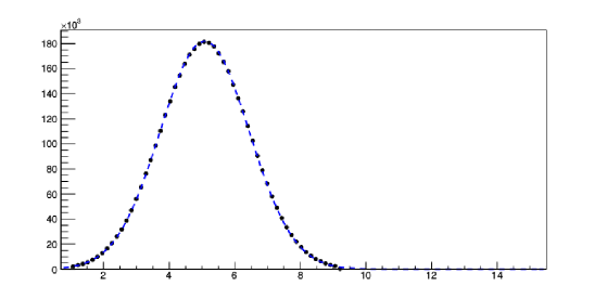
Dealing with asymmetric errors requires special care^[17,18]. After the symmetrization following the prescriptions in Ref. AssymError , making the results approximately symmetric and Gaussian (Fig.III.1):

$$(d\sigma/dE_{T}^{\gamma})_{\mathrm{exp}}=\sigma_{\mathrm{exp}}\pm\Delta_{\mathrm{exp}},$$ (III.2)

we propagate the experimental uncertainties by means of a series of pseudo-experiments using Monte Carlo technique as we will see in next section.

Figure III.1: An example of Gaussian distributions generated by the Monte Carlo method corresponding to the first data point $(5.09\pm 1.36)$ (nb/GeV) in the range $15<E_{T}^{\gamma}<20$ GeV and $|\eta^{\gamma}|<0.6$. The original (asymmetrical) value is $5.24_{-1.4}^{+1.3}(\mathrm{total})\pm 0.58(\mathrm{luminosity})$${}^{[6]}.$The $x$-axis represents $d\sigma/dE_{T}^{\gamma}$ in (nb/GeV) and the $y$-axis the number of entries.

The nominal values

The value of alphas is obtained, in each of the 79 $(|\eta^{\gamma}|\mathrm{-}E_{T}^{\gamma})$-bins of the measurement, by combining the theoretical calculations (II.2-II.5) and the $N=10^{7}$ MC generated experimental cross sections (III.2): a set of values $\left\{\alpha_{ik}\right\}$ are obtained for each $(|\eta^{\gamma}|\mathrm{-}E_{T}^{\gamma})$-bin, by means of pseudo-experiments where the experimental cross section corresponding to the bin is assumed to be Gaussian, and then a set of cross sections $\left\{\left(d\sigma/dE_{T}^{\gamma}\right)_{ik}\right\}$ is generated using Toy Monte Carlo techniques. Each of them is used to extract $\alpha_{ik}$ from the theoretical curves (II.2) using the linear inter(extra)polation numerical method.

The nominal value is represented by the average of the resulting sample$\left\{\alpha_{ik}\right\}$ :

$$\bar{\alpha}_{\mathrm{\mathit{i}}}=\frac{1}{N}\sum_{k=1}^{N}\alpha_{ik},\quad\mathrm{\mathit{i}\mathit{=\mathrm{1,...,79.}}}$$ (III.3)

The $\pm\sigma$ error is calculated using the CL=68% confidence interval for the mean. This is achieved by solving the following equation:

$$\intop_{\bar{\alpha}_{\mathrm{\mathit{i}}}-\Delta_{i}}^{\bar{\alpha}_{\mathrm{\mathit{i}}}+\Delta_{i}}dx\>\mathrm{pdf}_{i}(x)=\mathrm{CL}\simeq 0.6827;$$ (III.4)

where $\mathrm{pdf_{i}}(x)$ is the probability density function representing the sample $\left\{\alpha_{ik}\right\}$.

The Fig.III.2 shows several examples of $\alpha_{s}$distributions extracted from pseudo-experiments in several $(|\eta^{\gamma}|\mathrm{-}E_{T}^{\gamma})$-bins.

(a) $\begin{array}[]{c}15<E_{T}^{\gamma}<20\>\mathrm{GeV}\\ \left|\eta^{\gamma}\right|<0.6\end{array}$

(b) $\begin{array}[]{c}30<E_{T}^{\gamma}<35\>\mathrm{GeV}\\ \left|\eta^{\gamma}\right|<0.6\end{array}$

(c) $\begin{array}[]{c}45<E_{T}^{\gamma}<55\>\mathrm{GeV}\\ 0.6<\left|\eta^{\gamma}\right|<1.37\end{array}$

(d) $\begin{array}[]{c}60<E_{T}^{\gamma}<100\>\mathrm{GeV}\\ 0.6<\left|\eta^{\gamma}\right|<1.37\end{array}$

(e) $\begin{array}[]{c}200<E_{T}^{\gamma}<400\>\mathrm{GeV}\\ 0.6<\left|\eta^{\gamma}\right|<1.37\end{array}$

(f) $\begin{array}[]{c}500<E_{T}^{\gamma}<600\>\mathrm{GeV}\\ 1.52<\left|\eta^{\gamma}\right|<2.37\end{array}$

(g) $\begin{array}[]{c}800<E_{T}^{\gamma}<1000\>\mathrm{GeV}\\ \left|\eta^{\gamma}\right|<1.37\end{array}$.

Figure III.2: Examples of $\alpha_{s}$ probability distributions constructed from data generated by pseudo-experiments in different kinematic range. The $x$-axis represents $\alpha_{s}\left(M_{Z}^{2}\right)$ and the $y$-axis the number of entries.

The averaging procedure

To obtain the average value of the strong coupling from nominal values extracted in individual $(|\eta^{\gamma}|\mathrm{-}E_{T}^{\gamma})$ bin, we must take into account their correlations. For this purpose we used the Best Linear Unbiased Estimate (BLUE) method^[19] where the unbiased estimate $\hat{\alpha}$, is a linear combination of the individual estimates,

$$\hat{\alpha}= \sum_{i=1}^{79}\lambda_{i}\bar{\,\alpha_{i}}$$ (III.5)

with the constraint

$$\sum_{i=1}^{79}\lambda_{i}=1,$$ (III.6)

having the minimum variance $\sigma^{2}$:

$$\sigma^{2}=\sum_{ij=1}^{79}\lambda_{i}\mathrm{\,Cov_{\mathit{ij}\,}\lambda_{j},}$$ (III.7)

$\mathrm{Cov_{\mathit{ij}}}$ represents the covariance matrix elements.

The combination of the correlated estimates requires knowledge of the correlations between the different bins, but none of this information is available in the published experimental papers^[7,8,9] and the extraction of these correlations needs full access to all the uncertainties that contribute to the measurement of cross-sections.

Nevertheless, we have estimated the $79\times 79$ “nominal” covariance matrix using samples $\left\{\alpha_{ik}\right\}$:

$$\mathrm{Cov_{\mathit{ij}}}\simeq \frac{1}{N}\sum_{k=1}^{N}\left(\bar{\alpha}_{\mathrm{\mathit{i}}}-\alpha_{ik}\right)\left(\bar{\alpha}_{\mathrm{\mathit{j}}}-\alpha_{jk}\right),\>\mathrm{for}\>i\neq j;$$ (III.8)

$$\mathrm{Cov_{\mathit{ii}}}= \Delta_{i}^{2},$$

this is the sample covariance matrix, an unbiased estimate of the covariance matrix.

To be “conservative” the off-diagonal “nominal” covariance matrix elements (III.8) are multiplied by a factor in order to maximize the variance of the combined results^[20]:

$$\mathrm{Cov_{\mathit{ij}}} \rightarrow f\,\mathrm{Cov_{\mathit{\mathit{ij}}},}\>\mathrm{for}\>i\neq j;$$ (III.9)

where:

$$0\leq f\leq 1.$$ (III.10)

This procedure is implemented in a software package^[21] which is incorporated as part of ROOT analysis framework^[22].

For CT10wnlo PDFs and the scale choice (II.1), the average procedure yields the following BLUE value:

$$\alpha_{s}(M_{Z}^{2})_{\mathrm{CTEQ}}=0.1185\pm 0.0010\left(\mathrm{exp}.\right).$$ (III.11)

The scale uncertainty

The scale effect on the cross sections is studied in Ref. note CERN (Fig.10) and Ref. note ATL (Fig.5). These bands are evaluated by varying the three scales following the constraints:

• $\mu_{R}=\mu_{F}=\mu_{f}\in[\frac{1}{2}E_{T}^{\gamma},2E_{T}^{\gamma}];$

• $\mu_{R}\text{$\in$}[\frac{1}{2}E_{T}^{\gamma},2E_{T}^{\gamma}];\mu_{F}=\mu_{f}=\mathrm{E_{T}^{\gamma}};$

• $\mu_{F}\text{$\in$}[\frac{1}{2}E_{T}^{\gamma},2E_{T}^{\gamma}];\mu_{R}=\mu_{f}=\mathrm{E_{T}^{\gamma}};$

• $\mu_{f}\text{$\in$}[\frac{1}{2}E_{T}^{\gamma},2E_{T}^{\gamma}];\mu_{R}=\mu_{F}=\mathrm{E_{T}^{\gamma}};$

The scale uncertainty on the cross section is propagated to the uncertainty on $\alpha_{s}$ using the coefficients $\varGamma_{\mathrm{{}_{min}^{max}}}$ extracted from the figures cited above (see Tables 1):

$E_{T}^{\gamma}$-bin (GeV)	$\Gamma_{\mathrm{max}}$	$\Gamma_{\mathrm{min}}$
15-20	1.20	0.86
20-25	1.19	0.87
25-30	1.16	0.87
30-35	1.18	0.87
35-40	1.16	0.88
40-50	1.14	0.89
50-60	1.14	0.90
60-100	1.12	0.90

$E_{T}^{\gamma}$-bin (GeV)	$\Gamma_{\mathrm{max}}$	$\Gamma_{\mathrm{min}}$
45-55	1.14	0.89
55-70	1.13	0.90
70-85	1.12	0.90
85-100	1.12	0.91
100-125	1.12	0.91
125-150	1.12	0.90
150-200	1.12	0.90
200-400	1.12	0.90

(a) $\Gamma_{\mathrm{{}_{min}^{max}}}$ extracted from Fig. 10 of Ref. note CERN .

$E_{T}^{\gamma}$-bin (GeV)	$\Gamma_{\mathrm{max}}$	$\Gamma_{\mathrm{min}}$
100-125	1.059	0.956
125-150	1.065	0.952
150-175	1.068	0.950
175-200	1.070	0.949
200-250	1.068	0.949
250-300	1.063	0.951
300-350	1.054	0.955
350-400	1.043	0.960
400-500	1.038	0.962
500-600	1.048	0.960
600-700	1.061	0.912
700-800	1.076	0.820
800-1000	1.152	0.646

$E_{T}^{\gamma}$-bin (GeV)	$\Gamma_{\mathrm{max}}$	$\Gamma_{\mathrm{min}}$
100-125	1.076	0.943
125-150	1.084	0.937
150-175	1.091	0.932
175-200	1.095	0.928
200-250	1.098	0.926
250-300	1.100	0.923
300-350	1.085	0.927
350-400	1.067	0.934
400-500	1.067	0.934
500-600	1.055	0.955

(b) $\Gamma_{\mathrm{{}_{min}^{max}}}$ extracted from Fig. 5 of Ref. note ATL .

Table 1: Scale ratio coefficients $\Gamma_{\mathrm{{}_{min}^{max}}}$in different kinematic range.

$$\varGamma_{\mathrm{{}_{min}^{max}}}=\left(d\sigma_{\mu}/d\sigma_{\mu=\mu_{R}=\mu_{F}=\mu_{f}=E}\right)_{\mathrm{{}_{min}^{max}}}.$$ (III.12)

These values are related to MSTW2008 NLO set, but we can use them to evaluate the scale uncertainty related to CT10 set because the cross sections calculated with both sets are very close to each other (see Table 2).

To be “conservative”, the extreme values in each bin are considered, corresponding to the largest uncertainty.

Each theoretical curve $f_{\mathrm{bin}}$ (Eq. 2) generates two additional curves $f_{\mathrm{{}_{min}^{max}}}$ by rescaling cross sections with corresponding amounts $\varGamma_{\mathrm{{}_{min}^{max}}}$ and the nominal value of the corresponding measured cross section was mapped to the $(\bar{\alpha}_{i})_{\mathrm{min}}^{\mathrm{max}}$ .

The average procedure cited above gives two values $\alpha_{s}^{\mathrm{max}}$ and $\alpha_{s}^{\mathrm{min}}$ around the central one $0.1185$:

$$\alpha_{s}^{\mathrm{max}} =0.1221$$ (III.13)

$$\alpha_{s}^{\mathrm{min}} =0.1175$$ (III.14)

and then:

$$\alpha_{s}=0.1185_{-0.0010}^{+0.0036},$$ (III.15)

The scale uncertainty is consistent with LHC works determining $\alpha_{s}$ using jet data^[24].

The PDF uncertainties

CTEQ eign.

The JETPHOX error band cross sections calculated with CT10wnlo, involving 52 member PDFs, are combined with our theoretical curves (II.2) to estimate PDF uncertainties.

The weighted average procedure gives:

$$\bar{\alpha}_{\mathrm{CT10}}=0.1139\pm 0.0028$$ (III.16)

with a relative error of roughly $\frac{0.0028}{0.1139}\times 100=2.5\%$. The PDF-eign. uncertainty is estimated as:

$$\Delta_{\mathrm{PDF\,eig}.}^{\mathrm{CTEQ}}=\pm 0.025*0.1185=\pm 0.0029.$$ (III.17)

This value agrees with results obtained from LHC jet data studies^[24].

MSTW and CTEQ

We exploit informations on the cross section ratio $\varPi=d\sigma_{\mathrm{MSTW}}/d\sigma_{\mathrm{CTEQ}}$ extracted from tables 1-2 of Ref. note CERN and Fig.4 of Ref. ATLAS3 . We remark that there is no significant difference between cross section values calculated with MSTW and CTEQ pdfs (see Table2).

The ratio $\varPi$ is used to calculate the MSTW central value of $\alpha_{s}$:

$$\alpha_{s}(M_{Z}^{2})_{\mathrm{MSTW}}=0.1181\pm 0.0009\left(\mathrm{exp}.\right),$$ (III.18)

then:

$$\alpha_{s}(M_{Z}^{2})_{\mathrm{CTEQ}}-\alpha_{s}(M_{Z}^{2})_{\mathrm{MSTW}}=0.0004.$$ (III.19)

At this stage, we can write:

$$\alpha_{s}(M_{Z}^{2})=0.1183\pm 0.0002\left(\mathrm{\mathrm{MSTW-CTEQ}}\right)\pm 0.0029\left(\mathrm{CTEQ\,eig.}\right).$$ (III.20)

$E_{T}^{\gamma}$-bin (GeV)	$\varPi_{\left|\eta^{\gamma}\right|<0.6}$	$\varPi_{0.6<\left|\eta^{\gamma}\right|<1.37}$	$\varPi_{1.52<\left|\eta^{\gamma}\right|<1.81}$
15-20	1.027	1.024	1.023
20-25	1.041	1.040	1.033
25-30	1.046	1.050	1.043
30-35	1.063	1.050	1.052
35-40	1.036	1.049	1.048
40-50	1.055	1.043	1.052
50-60	1.059	1.062	1.042
60-100	1.083	1.067	1.000

$E_{T}^{\gamma}$-bin (GeV)	$\varPi_{\left|\eta^{\gamma}\right|<0.6}$	$\varPi_{0.6<\left|\eta^{\gamma}\right|<1.37}$	$\varPi_{1.52\leq\left|\eta^{\gamma}\right|<1.81}$	$\varPi_{1.81\leq\left|\eta^{\gamma}\right|<2.37}$
45-55	1.052	1.050	1.046	1.041
55-70	1.055	1.053	1.047	1.041
70-85	1.058	1.055	1.048	1.040
85-100	1.060	1.056	1.048	1.037
100-125	1.060	1.054	1.054	1.037
125-150	1.067	1.062	1.029	1.036
150-200	1.040	1.031	1.000	1.000
200-400	1.000	1.000	1.000	1.000

(a) $\varPi$ extracted from tables 1-2 of Ref. note CERN .

$E_{T}^{\gamma}$-bin (GeV)	$\varPi_{\left|\eta^{\gamma}\right|<1.37}$
100-125	1.038
125-150	1.050
150-175	1.047
175-200	1.105
200-250	1.037
250-300	1.032
300-350	1.043
350-400	1.028
400-500	1.048
500-600	1.020
600-700	1.021
700-800	1.012
800-1000	0.991

$E_{T}^{\gamma}$-bin (GeV)	$\varPi_{1.52\leq\left|\eta^{\gamma}\right|<2.37}$
100-125	1.046
125-150	1.018
150-175	1.031
175-200	1.001
200-250	0.998
250-300	1.019
300-350	1.023
350-400	1.036
400-500	0.951
500-600	1.010

(b) $\varPi$ extracted from Fig.4 of Ref. ATLAS3 .

Table 2: The ratio of cross sections $\varPi$ corresponding to CTEQ and MSTW pdfs, in different kinematic range.

The $\alpha_{s}$value

Finally our estimation of the $\alpha_{s}(M_{Z}^{2})$, including experimental, PDF and scale errors is:

$$\alpha_{s}(M_{Z}^{2}) =0.1183\pm 0.0010(\mathrm{exp.})\pm_{0.0010}^{0.0036}(\mathrm{scale})\pm 0.0002(\mathrm{MSTW\mathrm{-}CT10\>PDF})\pm 0.0029(\mathrm{CT10\>eig.})$$ (III.21)

$$\alpha_{s}(M_{Z}^{2}) =0.1183\pm 0.0038.$$

This result is consistent with the recent PDG average world value $0.1181\pm 0.0011$^[2], and with values extracted directly from jet measurements at the LHC^[24], especially with the value reported by CMS Collaboration^[23]: $0.1185\pm 0.0019\>(\mathrm{exp})\pm 0.0028\>(\mathrm{PDF})\pm 0.0004\>(\mathrm{NP})\pm 0.0024\>(\mathrm{scale})$.

IV Conclusion

Using the measured inclusive isolated prompt photon production cross sections reported by ATLAS Collaboration at $\sqrt{s}=7$ TeV combined with Monte Carlo NLO calculations, we propose for the first time an estimation of the strong coupling constant exploiting the prompt photon production process, up to TeV region. Both theoretical and experimental errors are evaluated and our result has been determined to be $\alpha_{s}\left(M_{Z}^{2}\right)=0.1183\pm 0.0038\>(\mathrm{exp.,PDF},\mathrm{scale})$, which is in good agreement with the most recent world average value $0.1181\pm 0.0011$^[2].

It is important to note that the theoretical uncertainties are mostly coming from terms beyond NLO order. The calculations of prompt photon production cross sections to NNLO are necessary to overcome this deficiency, especially they will minimize the sensitivity of the result to the scale parameters and will improve accuracy in $\alpha_{s}$ determination.

V Acknowledgements

This work was realized with the support of the FNR (Algerian Ministry of Higher Education and Scientific Research), as part of the research project D018 2014 0044. The authors are grateful to Olivier Pène and Michel Fontannaz for many useful discussions on this work; and we thank the laboratory of theoretical physics (LPT, Université Paris-Sud, Orsay) for its warm hospitality during our visits there. In addition, we gratefully acknowledge the UCI Computing Centre of Oran-1 University and its Staff for delivering so effectively the computing infrastructure essential to our work.

References

• (1) D. Becciolini, M. Gillioz, F. Sannino, M. Nardecchia, and M. Spannowsky, Phys. Rev. D 91, 015010 (2015); Erratum Phys. Rev. D 92, 079905(E) (2015).
• (2) S. Bethke, G. Dissertori and G.P. Salam ,โ€9.4. Determinations of the strong coupling constantโ€; (2016 Review of Particle Physics), Chin. Phys. C40, 100001 (2016).
• (3) y S. Hashimo, J. Laiho and S.R. Sharpe,โ€18.3.4. Strong coupling constantโ€; (2016 Review of Particle Physics), Chin. Phys. C40, 100001 (2016).
• (4) B. Blossier, Ph. Boucaud, M. Brinet, F. De Soto, V. Morenas, O. Pรจne, K. Petrov, J. Rodrรญguez-Quintero, Phys. Rev. D 89, 014507 (2014).
• (5) Juan Rojo, arXiv:1410.7728.
• (6) CMS collaboration, Phys. Lett. B 728, 496 (2013).
• (7) G. Aad et al. (ATLAS Collaboration), Phys. Rev. D 83, 052005 (2011).
• (8) ATLAS Collaboration, Phys. Lett. B 706, 150 (2011).
• (9) G. Aad et al. (ATLAS Collaboration), Phys. Rev. D 89, 052004 (2014).
• (10) S. Catani, M. Fontannaz, J-P. Guillet and E. Pilon, JHEP 05, 028 (2002); http://lapth.cnrs.fr/PHOX_FAMILY/.
• (11) H.-L. Lai, M. Guzzi, J. Huston, Z. Li, P.M. Nadolsky, J. Pumplin, and C.-P. Yuan, Phys. Rev. D 82, 074024 (2010).
• (12) M.R.Whalley, D.Bourilkov and R.C.Group, arXiv:hep-ph/0508110; http://lhapdf.hepforge.org.
• (13) Blair R. Brelier B., Bucci F., Chekanov S., Stockton M. and Tripiana M., CERN-OPEN-2011-041.
• (14) The ATLAS collaboration, ATL-PHYS-PUB-2013-018.
• (15) T. Sjรถstrand, S. Mrenna and P. Z. Skands, JHEP 05 026 (2006).
• (16) CMS collaboration, Phys. Rev. D 84, 052011 (2011).
• (17) G. Dโ€™Agostini, arXiv:physics/0403086.
• (18) R. Barlow, ECONF C030908:WEMT002(2003); arXiv:physics/0401042v1.
• (19) L. Lyons and D. Gibaut and P. Cliord, Nucl. Instr. and Meth. A270 (1988) 110.
• (20) A. Valassi and R., arXiv:1307.4003
• (21) R. Nisius, URL http: //blue.hepforge.org.
• (22) R. Brun and F. Rademakers, Nucl. Instr. and Meth. A389, 81 (1997). Proceedings of AIHENPโ€™96 Workshop, Lausanne, Sep. 1996.
• (23) V. Khachatryan et al. (CMS Collaboration), Eur. Phys. J. C 75, 288 (2015); arXiv:1410.6765 [hep-ex].
• (24) D. dโ€™Enterria et al. , arXiv:1512.05194 [hep-ph]