Generalized Rao Test for Decentralized Detection of an Uncooperative Target

Abstract

We tackle distributed detection of a non-cooperative target with a Wireless Sensor Network (WSN). When the target is present, sensors observe an (unknown) deterministic signal with attenuation depending on the distance between the sensor and the (unknown) target positions, embedded in symmetric and unimodal noise. The Fusion Center (FC) receives quantized sensor observations through error-prone Binary Symmetric Channels (BSCs) and is in charge of performing a more-accurate global decision. The resulting problem is a two-sided parameter testing with nuisance parameters (i.e. the target position) present only under the alternative hypothesis. After introducing the Generalized Likelihood Ratio Test (GLRT) for the problem, we develop a novel fusion rule corresponding to a Generalized Rao (G-Rao) test, based on Davies’ framework, to reduce the computational complexity. Also, a rationale for threshold-optimization is proposed and confirmed by simulations. Finally, the aforementioned rules are compared in terms of performance and computational complexity.

I Introduction

Wireless Sensor Networks (WSNs) have attracted significant interest due to their applicability to reconnaissance, surveillance, security and environmental monitoring [1]. Distributed detection is one of the main tasks for a WSN and it has been heavily investigated in the last decades [2].

Due to stringent bandwidth and energy constraints, it is often assumed that each sensor sends one bit of information about the estimated hypothesis to the Fusion Center (FC). In this context the optimal test (under Bayesian/Neyman-Pearson frameworks) at each sensor is known to be a one-bit quantization of the local Likelihood-Ratio (LR); that is to perform a LR Test (LRT). Unfortunately in most cases, due to a lack of knowledge of the parameters of the target to be detected, it is not possible to compute the LRT at each sensor. Also, even when the sensors can compute their local LRT, the search for local quantization thresholds is exponentially complex [3, 4]. Thus the bit of information being sent is usually the result of a “dumb” quantization [5, 6] or represents the estimated binary event, according to a sub-optimal rule [7, 8]. In both cases, the bits from the sensors are collected by the FC and combined via a specifically-designed fusion rule aiming at improved detection rate.

The optimum strategy to fuse the sensors’ bits at the FC, under conditional independence assumption, is a weighted sum, with weights depending on unknown target parameters [2]. Some simple fusion approaches, based on the counting rule or channel-aware statistics, have been proposed in the literature to overcome such unavailability [9, 10, 11, 12]. On the other hand, in some particular scenarios the uniformly most powerful test is independent of the unknown parameters under the alternative hypothesis, so they do not need to be estimated [13]. Nonetheless, in the general case the FC is usually in charge of solving a composite hypothesis test and the Generalized LRT (GLRT) is commonly employed [14]. Indeed, GLRT-based fusion of quantized data was studied in [15, 6, 16] for: ($i$) detecting a known source with unknown location, ($ii$) detecting an unknown source with known observation coefficients, and $(iii)$ fusing conditionally dependent decisions, respectively. As a simpler alternative, a Rao test was developed in a more general context for problem $(ii)$ in [5]. However, in the case of an uncooperative target, it is reasonable to assume that both the target emitted signal and location are not available at the FC. To the best of authors’ knowledge, only a few works have dealt with the latter case [17, 18]. In [17], a GLRT was derived for revealing a target with unknown position and emitted power and compared to the so-called counting rule, the optimum rule and a GLRT based on the awareness of target emitted power, showing a marginal loss of the latter rule with respect to the “power-clairvoyant” GLRT. Unfortunately, the considered GLRT requires a grid search on both the target location and emitted power domains. Therefore, as a computationally simpler solution, generalized forms of locally-optimum detectors have been proposed for non-cooperative detection of a fluctuating target emission [18].

In this letter, we focus on decentralized detection of a non-cooperative target with a spatially-dependent emission (signature), with emitted signal modelled as unknown and deterministic (as opposed to [18]). More specifically, the received signal at each individual sensor is embedded in unimodal zero-mean additive noise, with a deterministic Amplitude Attenuation Function (AAF) depending on the sensor-target distance. Each sensor observes a local measurement on the absence/presence of the target and forwards a single bit version to a FC, over noisy imperfect (modelled as Binary Symmetric Channels, BSCs) reporting channels, which is in charge of providing an accurate global decision. The problem considered is a two-sided parameter test with nuisance parameters present only under the alternative hypothesis, which thus precludes the application of conventional score-based tests, such as the Rao test. In order to reduce the computational complexity required by the GLRT, we develop a (simpler) sub-optimal fusion rule based on a generalization of the Rao test [14]. The aforementioned detector is also compared in terms of computational complexity. Finally, simulation results are provided to compare these rules in some practical scenarios.

The letter is organized as follows: Sec. II describes the system model; Sec. III develops the generalized form of Rao test and tackles the quantizer optimization problem, with results validated in Sec. IV. Finally, conclusions are in Sec. VI.

II System Model

We consider a binary hypothesis test where a collection of sensors $k\in\mathcal{K}\triangleq\{1,\ldots,K\}$ are deployed in a surveillance area to monitor the absence ($\mathcal{H}_{0}$) or presence ($\mathcal{H}_{1}$) of a target of interest having a partially-specified spatial signature. The problem can be summarized as follows:

$$\begin{cases}\mathcal{H}_{0}\quad:\quad&y_{k}=w_{k},\\ \mathcal{H}_{1}\quad:\quad&y_{k}=\theta\,g(\bm{x}_{T},\bm{x}_{k})+w_{k},\qquad k\in\mathcal{K};\end{cases}$$ (1)

In other terms, when the target is present (i.e. $\mathcal{H}_{1}$), we assume that its radiated (amplitude) signal $\theta$, modelled as unknown deterministic, is isotropic and experiences (distance-dependent) path-loss and additive noise, before reaching individual sensors. In Eq. (1), $y_{k}\in\mathbb{R}$ denotes the $k$th sensor measurement and $w_{k}\in\mathbb{R}$ denotes the noise Random Variable (RV) with $\mathbb{E}\{w_{k}\}=0$ and unimodal symmetric pdf, denoted with $p_{w_{k}}(\cdot)$ (the RVs $w_{k}$ are assumed mutually independent). Additionally, $\bm{x}_{T}\in\mathbb{R}^{d}$ denotes the unknown position of the target, while $\bm{x}_{k}\in\mathbb{R}^{d}$ denotes the known $k$th sensor position. Both $\bm{x}_{T}$ and $\bm{x}_{k}$ uniquely determine the value of $g(\bm{x}_{T},\bm{x}_{k})$, generically denoting the AAF.

For example, the measurement $y_{k}$ is distributed under $\mathcal{H}_{0}$ (resp. $\mathcal{H}_{1}$) as $y_{k}\,|\,\mathcal{H}_{0}\sim\mathcal{N}(0,\sigma_{w,k}^{2})$ (resp. $y_{k}\,|\,\mathcal{H}_{1}\sim\mathcal{N}(\theta\,g(\bm{x}_{T},\bm{x}_{k}),\,\sigma_{w,k}^{2})$) when the noise is modelled as $w_{k}\sim\mathcal{N}(0,\sigma_{w}^{2})$. Then, to meet stringent bandwidth and energy budgets in WSNs, the $k$th sensor quantizes $y_{k}$ into one bit of information, i.e. $b_{k}\triangleq u\,(y_{k}-\tau_{k})$, $k\in\mathcal{K}$, where $\tau_{k}$ denotes the quantizer threshold. The bit $b_{k}$ is sent over a BSC and the FC observes an error-prone version due to non-ideal transmission, i.e. $\hat{b}_{k}=b_{k}$ (resp. $\hat{b}_{k}=(1-b_{k})$) with probability $(1-P_{e,k})$ (resp. $P_{e,k}$), which we collect as $\hat{\bm{b}}\triangleq\left[\begin{array}[]{ccc}\hat{b}_{1}&\cdots&\hat{b}_{K}\end{array}\right]^{T}$. Here $P_{e,k}$ denotes the (known) BEP of $k$th link.

We underline that the unknown target position $\bm{x}_{T}$ is observable (i.e. can be estimated) at the FC only when the signal is present, i.e. $\theta\neq\theta_{0}$ ($\theta_{0}=0$). Therefore, the problem in Eq. (1) refers to a two-sided parameter test (that is $\{\mathcal{H}_{0},\mathcal{H}_{1}\}$ corresponds to $\{\theta=\theta_{0},\theta\neq\theta_{0}\}$) with nuisance parameters ($\bm{x}_{T}$) present only under the alternative hypothesis $\mathcal{H}_{1}$ [19]. The aim of this study is the derivation of a (computationally) simple test deciding in favour of $\mathcal{H}_{1}$ (resp. $\mathcal{H}_{0}$) when the statistic $\Lambda(\hat{\bm{b}})$ is above (resp. below) the threshold $\gamma$, and the quantizer design for each sensor (i.e. an optimized $\tau_{k}$, $k\in\mathcal{K}$).

III Fusion Rules

III-A Test derivation

A common approach for composite hypothesis testing is given by the GLRT [17], whose expression is:

$$\Lambda_{\mathrm{G}}\triangleq 2\,\ln[P(\hat{\bm{b}};\hat{\theta}_{1},\widehat{\bm{x}}_{T})\,/\,P(\hat{\bm{b}};\theta_{0})]$$ (2)

where $P(\hat{\bm{b}};\theta,\bm{x}_{T})$ denotes the likelihood as a function of $(\theta,\bm{x}_{T})$, whereas $\hat{\theta}_{1}$ and $\widehat{\bm{x}}_{T}$ are the Maximum Likelihood (ML) estimates under $\mathcal{H}_{1}$ (i.e. $(\hat{\theta}_{1},\widehat{\bm{x}}_{T})\triangleq\arg\max_{(\theta,\bm{x}_{T})}P(\hat{\bm{b}};\theta,\bm{x}_{T})$). It is clear from Eq. (2) that $\Lambda_{\mathrm{G}}$ requires the solution to an optimization problem. Unfortunately a closed form for the pair $(\hat{\theta}_{1},\widehat{\bm{x}}_{T})$ is not available even for Gaussian noise. This increases the computational complexity of its implementation, which typically involves a grid approach on ($\theta,\bm{x}_{T}$), see e.g. [17].

A different path for exploiting the two-sided nature of the problem consists in adopting the rationale in [19]. This allows to extend score-based tests to the case of nuisance parameters present solely under $\mathcal{H}_{1}$. Indeed, score-based tests require the ML estimates of nuisances under $\mathcal{H}_{0}$ [14], which thus cannot be obtained, as they are not observable. The cornerstone of Davies’ work is summarized as follows. If $\bm{x}_{T}$ were known in (1), it would be easy to find a simple test for a two-sided testing: indeed, in the latter case, the Rao test seems a reasonable decision procedure [14]. However, since $\bm{x}_{T}$ is unknown in our setup, a family of statistics is instead obtained by varying $\bm{x}_{T}$. Thus, to overcome this technical difficulty, Davies proposed the use of the maximum of the resulting family of the statistics, following a “GLRT-like” approach. In what follows, we will refer to the employed decision test as Generalized Rao (G-Rao), to underline the use of Rao as the inner statistic employed in Davies approach, that is:

$$\Lambda_{\mathrm{R}}\,\triangleq\, \max_{\bm{x}_{T}}\left.\left(\frac{\partial\ln P(\hat{\bm{b}};\theta,\bm{x}_{T})}{\partial\theta}\right)^{2}\right|_{\theta=\theta_{0}}/\>\mathrm{I}(\theta_{0},\bm{x}_{T}),$$ (3)

where $\mathrm{I}(\theta,\bm{x}_{T})\triangleq\mathbb{E}\{\left(\frac{\partial\ln\left[P(\hat{\bm{b}};\theta,\bm{x}_{T})\right]}{\partial\theta}\right)^{2}\}$ is the Fisher Information (FI) obtained assuming $\bm{x}_{T}$ is known, evaluated at $\theta_{0}$ in (3). Our choice is motivated by reduced complexity of test implementation (since $\hat{\theta}_{1}$ is not required, cf. Eq. (3), and thus a grid implementation w.r.t. the sole $\bm{x}_{T}$ is required).

In order to obtain $\Lambda_{\mathrm{R}}$ explicitly, exploiting the independence of sensors’ measurements and reporting channels, we expand $\ln\left[P(\hat{\bm{b}};\theta,\bm{x}_{T})\right]$ as:

$$\ln\left[P(\hat{\bm{b}};\theta,\bm{x}_{T})\right]=\sum_{k=1}^{K}\ln\left[P(\hat{b}_{k};\theta,\bm{x}_{T})\right]=$$

$$\sum_{k=1}^{K}\{\hat{b}_{k}\,\ln\left[\alpha_{k}(\theta,\bm{x}_{T})\right]+(1-\hat{b}_{k})\,\ln\left[1-\alpha_{k}(\theta,\bm{x}_{T})\right]\}$$ (4)

where $\alpha_{k}(\theta,\bm{x}_{T})\triangleq(1-P_{e,k})\beta_{k}(\theta,\bm{x}_{T})+P_{e,k}(1-\beta_{k}(\theta,\bm{x}_{T}))$ and $\beta_{k}(\theta,\bm{x}_{T})\triangleq F_{w_{k}}(\tau_{k}-\theta g(\bm{x}_{T},\bm{x}_{k}))$, $F_{w_{k}}(\cdot)$ being the complementary cumulative distribution function of $w_{k}$. On the other hand, the closed form of $\mathrm{I}(\theta,\bm{x}_{T})$ is [6, 5]:

$$\mathrm{I}(\theta,\bm{x}_{T})=\sum_{k=1}^{K}\psi_{k}(\theta,\bm{x}_{T})\,g(\bm{x}_{T},\bm{x}_{k})^{2}\,,$$ (5)

where

$$\psi_{k}(\theta,\bm{x}_{T})\triangleq\frac{(1-2\,P_{e,k})^{2}\>p_{w_{k}}^{2}(\tau_{k}-\theta g(\bm{x}_{T},\bm{x}_{k}))}{\alpha_{k}(\theta,\bm{x}_{T})\,\left(1-\alpha_{k}(\theta,\bm{x}_{T})\right)}\,.$$ (6)

Plugging Eqs. (4-5) into (3), we obtain $\Lambda_{\mathrm{R}}$ explicitly as:

$$\Lambda_{\mathrm{R}}=\max_{\bm{x}_{T}}\frac{\left[\sum_{k=1}^{K}\nu_{k}(\hat{b}_{k})\,g(\bm{x}_{T},\bm{x}_{k})\right]^{2}}{\sum_{k=1}^{K}\psi_{k,0}\,g(\bm{x}_{T},\bm{x}_{k})^{2}},$$ (7)

where we have defined $\nu_{k}(\hat{b}_{k})\triangleq\frac{(1-2\,P_{e,k})\,p_{w_{k}}(\tau_{k})\,\left[\hat{b}_{k}-\alpha_{k,0}\right]}{\alpha_{k,0}(1-\alpha_{k,0})}$, $\alpha_{k,0}\triangleq\alpha_{k}(\theta_{0},\bm{x}_{T})$ and $\psi_{k,0}\triangleq\psi_{k}(\theta_{0},\bm{x}_{T})$. It is apparent that $\Lambda_{\mathrm{R}}$ (as well as $\Lambda_{\mathrm{G}}$) is a function of $\tau_{k}$ (as $\widehat{\nu}_{k}(\hat{b}_{k})$ and $\psi_{k,0}$ both depend on $\tau_{k}$), $k\in\mathcal{K}$, (collected as $\bm{\tau}\triangleq\begin{bmatrix}\tau_{1}&\cdots&\tau_{K}\end{bmatrix}^{T}$) which can be optimized to achieve improved performance.

III-B Quantizer Design

It is worth noticing that (asymptotically-) optimal deterministic quantizers cannot be obtained as in [6, 5], because no performance expressions are known in the literature for tests based on the Davies approach [19]. To this end, we adopt a modified version of the rationale in [6, 5] and then we confirm its validity by simulations in Sec. IV. Specifically, it is known that the (position $\bm{x}_{T}$) clairvoyant Rao statistic $\bar{\Lambda}_{\mathrm{R}}$ (as well as the corresponding clairvoyant GLR), is asymptotically (and assuming a weak signal) distributed as [14]

$$\bar{\Lambda}_{\mathrm{R}}\overset{{\scriptstyle a}}{\sim} \begin{cases}\chi_{1}^{2}&\quad\mathrm{under}\quad\mathcal{H}_{0}\\ \chi_{1}^{{}^{\prime}2}\left(\lambda_{Q}(\bm{x}_{T})\right)&\quad\mathrm{under}\quad\mathcal{H}_{1}\end{cases},$$ (8)

where the non-centrality parameter $\lambda_{Q}(\bm{x}_{T})\triangleq(\theta_{1}-\theta_{0})^{2}\,\mathrm{I}(\theta_{0},\bm{x}_{T})$ (underlining dependence on $\bm{x}_{T}$) is given as:

$$\lambda_{Q}(\bm{x}_{T}) =\theta_{1}^{2}\sum_{k=1}^{K}\psi_{k,0}\,g(\bm{x}_{T},\bm{x}_{k})^{2}\,,$$ (9)

with $\theta_{1}$ being the true value under $\mathcal{H}_{1}$. Clearly the larger $\lambda_{Q}(\bm{x}_{T})$, the better the $\bm{x}_{T}-$clairvoyant GLRT and Rao tests will perform when the target to be detected is located at $\bm{x}_{T}$. Also, it is apparent that $\lambda_{Q}(\bm{x}_{T})$ is a function of $\tau_{k}$, $k\in\mathcal{K}$ (because of the $\psi_{k,0}$’s). For this reason, with a slight abuse of notation we will use $\lambda_{Q}(\bm{x}_{T},\bm{\tau})$ and we choose the thresholds $\bm{\tau}$ to maximize $\lambda_{Q}(\bm{x}_{T},\bm{\tau})$, that is $\bm{\tau}^{\star}\triangleq\arg\max_{\bm{\tau}}\;\lambda_{Q}(\bm{x}_{T},\bm{\tau})$. In general, such optimization would lead to an optimized threshold that will be dependent on $\bm{x}_{T}$ (and thus not practical). However, for this specific problem the optimization can be decoupled into the following set of $K$ independent threshold design problems, which are independent of $\bm{x}_{T}$ (cf. Eq. (9)):

$$\arg\max_{\tau_{k}}\left\{\psi_{k,0}(\tau_{k})=\frac{p_{w_{k}}^{2}(\tau_{k})}{\Delta_{k}+F_{w_{k}}(\tau_{k})\left[1-F_{w_{k}}(\tau_{k})\right]}\right\}$$ (10)

where $\Delta_{k}\triangleq[P_{e,k}\,(1-P_{e,k})]/(1-2P_{e,k})^{2}$. It is known from the quantized estimation literature [20, 21] that many unimodal and symmetric $p_{w_{k}}(\cdot)$’s with $\mathbb{E}\{w_{k}\}=0$ lead to $\tau_{k}^{\star}\triangleq\arg\max_{\tau_{k}}\psi_{k,0}(\tau_{k})=0$ (independent of $\Delta_{k}$); such examples are the Gaussian, Laplace, Cauchy and the widely used generalized normal distribution (only in the case $0\leq\epsilon\leq 2$). Also, it has been shown in [5] that $\tau_{k}=0$ is still a good (sub-optimal) choice even when not corresponding to the optimizer for a specific noise pdf, especially in the case of noisy ($P_{e,k}\neq 0$) reporting channels. Therefore, we employ $\tau_{k}=0$, $k\in\mathcal{K},$ in Eq. (7), leading to the following further simplified expression for threshold-optimized G-Rao test (denoted with $\Lambda_{\mathrm{R}}^{\star}$):

$$\Lambda_{\mathrm{R}}^{\star}\triangleq\max_{\bm{x}_{T}}\frac{4\left[\sum_{k=1}^{K}(1-2\,P_{e,k})\,p_{w_{k}}(0)\,g(\bm{x}_{T},\bm{x}_{k})\,(\hat{b}_{k}-\frac{1}{2})\right]^{2}}{\sum_{k=1}^{K}(1-2\,P_{e,k})^{2}\,p_{w_{k}}^{2}(0)\,g(\bm{x}_{T},\bm{x}_{k})^{2}}$$ (11)

which is considerably simpler than the GLRT, as it obviates solution of a joint optimization problem w.r.t. $(\bm{x}_{T},\theta)$ (which depends on $p_{w_{k}}(\cdot)$). Furthermore, the corresponding optimized non-centrality parameter, denoted with $\lambda_{Q}^{\star}(\bm{x}_{T})$, is given by:

$$\lambda_{Q}^{\star}(\bm{x}_{T})\triangleq 4\theta_{1}^{2}\sum_{k=1}^{K}\left[(1-2\,P_{e,k})^{2}\,p_{w_{k}}^{2}(0)\,g(\bm{x}_{T},\bm{x}_{k})^{2}\right].$$ (12)

III-C Computational Complexity

As detailed in [15, 17, 18], the GLRT is usually implemented by means of a grid discretization. More specifically, assuming that $\bm{x}_{T}$ and $\theta$ belong to limited sets $\mathrm{S}_{\bm{x}_{T}}\subset\mathbb{R}^{d}$ and $S_{\mathrm{\theta}}\subset\mathbb{R}$, respectively, the search space ($\bm{x}_{T},\theta)$ required for (2) is then discretized into: ($a$) $N_{\bm{x}_{T}}$ position bins in $\mathbb{R}^{d}$, each one associated to a center bin position, say $\bm{x}_{T}[i]$, $i\in\{1,\ldots N_{\bm{x}_{T}}\}$; ($b$) $N_{\theta}$ amplitude bins in $\mathbb{R}$, each one to associated to a center bin amplitude, say $\theta[j]$, $j\in\{1,\ldots N_{\theta}\}$. Similarly, the G-Rao statistic is implemented by discretizing the sole search space of $\bm{x}_{T}$, leading to:

$$\Lambda_{\mathrm{R}}\approx\max_{i=1,\ldots N_{\bm{x}_{T}}}\frac{\left[\sum_{k=1}^{K}\nu_{k}(\hat{b}_{k})\,g(\bm{x}_{T}[i],\bm{x}_{k})\right]^{2}}{\sum_{k=1}^{K}\psi_{k,0}\,g(\bm{x}_{T}[i],\bm{x}_{k})^{2}}\,.$$ (13)

Thus, its complexity is $\mathcal{O}\left(K\,N_{\bm{x}_{T}}\right)$, thus providing a significant complexity reduction w.r.t. the GLR, as reported in Tab. I.

Table I: Complexity comparison of decision statistics.

Fusion Rule	Computational Complexity
GLR	$\mathcal{O}\left(K\,N_{\bm{x}_{T}}\,N_{\theta}\right)$ (Grid search)
G-Rao	$\mathcal{O}\left(K\,N_{\bm{x}_{T}}\right)$ (Grid search)

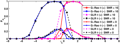
Figure 1: $P_{D_{0}}$ vs $\tau_{k}=\tau$, $P_{F_{0}}=0.01$; WSN with $K=49$ sensors, $P_{e,k}=0$, $\mathrm{SNR}\in\{0,10\}$ (amplitude signal with positive/negative polarity).

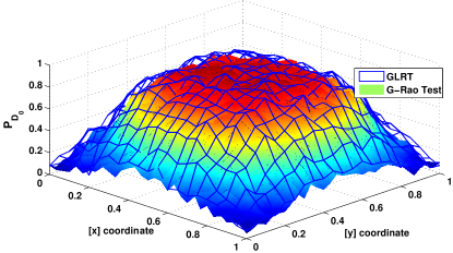
Figure 2: $P_{D_{0}}$ vs $\bm{x}_{T}$, $P_{F_{0}}=0.01$; WSN with $K=49$ sensors, $\tau_{k}=0$, $P_{e,k}=0$, $\mathrm{SNR=5\,\mathrm{dB}}$.

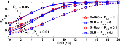
Figure 3: $P_{D_{0}}$ vs. $\mathrm{SNR}$ ($\mathrm{dB}$), $P_{F_{0}}\in\{0.05,0.01\}$; WSN with $K=49$ sensors, $\tau_{k}=0$, $P_{e,k}=P_{e}\in\{0,0.1\}$.

IV Gaussian noise Analysis

In this section we compare G-Rao and GLR tests, by evaluating their performance in terms of system false alarm and detection probabilities, defined as $P_{F_{0}}\triangleq\Pr\{\Lambda>\gamma|\mathcal{H}_{0}\}$ and $P_{D_{0}}\triangleq\Pr\{\Lambda>\gamma|\mathcal{H}_{1}\}$, respectively, where $\Lambda$ is the statistic employed at the FC. Additionally, we will validate the zero-threshold choice obtained in Sec. III-B.

To this end, we consider a 2-D scenario ($\bm{x}_{T}\in\mathbb{R}^{2}$) where a WSN composed of $K=49$ sensors is employed to detect the presence of a target within the (square) region $\mathcal{A}\triangleq[0,1]^{2}$, being the surveillance area. For simplicity the sensors are arranged according to a regular square grid covering $\mathcal{A}$. With reference to the sensing model, we assume $w_{k}\sim\mathcal{N}(0,\sigma_{w}^{2})$, $k\in\mathcal{K}$ (also w.l.o.g. we set $\sigma_{w}^{2}=1$). Also, the AAF chosen is $g(\bm{x}_{T},\bm{x}_{k})\triangleq 1\,/\,\sqrt{1+\left(\left\|\bm{x}_{T}-\bm{x}_{k}\right\|/\,\eta\right)^{\alpha}}$ (i.e. a power-law), where we have set $\eta=0.2$ (viz. approximate target extent) and $\alpha=4$ (viz. decay exponent). Finally, we define the target Signal-To-Noise Ratio (SNR) as $\mathrm{SNR}\triangleq 10\,\log_{10}(\theta^{2}/\sigma_{w}^{2})$. Initially, we assume ideal BSCs, i.e. $P_{e,k}=0$, $k\in\mathcal{K}$.

As explained before, $\Lambda_{\mathrm{G}}$ and $\Lambda_{\mathrm{R}}$ are implemented by means of grids for $\theta$ and $\bm{x}_{T}$. Specifically, the search space of the target signal $\theta$ is assumed to be $S_{\theta}\triangleq\left[-\bar{\theta},\bar{\theta}\right]$, where $\bar{\theta}>0$ is such that the $\mathrm{SNR}=20\,\mathrm{dB}$. The grid points are then chosen as $\begin{bmatrix}-\bm{g}_{\theta}^{T}&0&\bm{g}_{\theta}^{T}\end{bmatrix}^{T},$ where $\bm{g}_{\theta}$ collects target strengths corresponding to the SNR dB values $-10:1:20$ (thus $N_{\theta}=63$). Differently, the search space of the target position $\bm{x}_{T}$ is (naturally) assumed to coincide with the surveillance area, i.e. $\mathrm{S}_{\bm{x}_{T}}=\mathcal{A}$. The 2-D grid points are then obtained by regularly sampling $\mathcal{A}$ with $N_{\bm{x}_{T}}=N_{c}^{2}$ points, where $N_{c}=100$.

First, in Fig. 1 we show $P_{D_{0}}$ (under $P_{F_{0}}=0.01$) versus a common threshold choice for all the sensors $\tau_{k}=\tau$, $k\in\mathcal{K}$, for a target whose location is randomly drawn according to a uniform distribution within $\mathcal{A}$. It is apparent that in the low-SNR limit $\tau=0$ represents a nearly-optimal solution, since the optimal value of $\tau$ found numerically depends on the polarity of $\theta$, which is unknown. This both applies to GLR and G-Rao as well. Secondly, in Fig. 2, we report $P_{D_{0}}$ (under $P_{F_{0}}=0.01$) versus target location $\bm{x}_{T}$ (for $\mathrm{SNR}=5\,\mathrm{dB}$), in order to obtain a clear comparison of detection performance over the entire surveillance area $\mathcal{A}$. It is apparent that the G-Rao test presents only marginal loss over the GLRT. Additionally the $P_{D_{0}}(\bm{x}_{T})$ profile is qualitatively similar for both rules, and underlines lower detection performance at the boundaries of the surveillance area. This can be attributed to regular displacement of the WSN within $\mathcal{A}$. Finally, in Fig. 3 we compare the $P_{D_{0}}$ (for $P_{F_{0}}\in\{0.05,0.01\}$) of considered rules (for a target with randomly drawn position within $\mathcal{A}$) versus $\mathrm{SNR}$ ($\mathrm{dB}$), in order to obtain a comparison of detection sensitivity versus the signal strength. It is apparent that both rules perform very similarly over the whole SNR range, as well as for a different quality of the reporting channel ($P_{e,k}=P_{e}\in\{0,0.1\}$).

V Laplace noise Analysis

In this section the focus will be on $w_{k}$s modelled as Laplace noise. Similarly, we will validate the zero-threshold choice proposed in the paper also for this case. With reference to the sensing model, we assume $w_{k}\sim\mathcal{L}(0,\beta_{k})$, $k\in\mathcal{K}$ (here $\mathcal{L}(\mu,\beta)$ is used to denote a Laplace pdf with mean $\mu$ and scale parameter $\beta$). Also for simplicity, we assume that each $\beta_{k}$ is chosen such that $\mathrm{\mathbb{E}}\{w_{k}^{2}\}=1$. Furthermore, we define the target Signal-To-Noise Ratio (SNR) as $\mathrm{SNR}\triangleq 10\,\log_{10}(\theta^{2}/\mathrm{\mathbb{E}}\{w_{k}^{2}\})$. Initially, we assume ideal BSCs, i.e. $P_{e,k}=0$, $k\in\mathcal{K}$. Finally, we remark that we use the same grid implementation of GLRT and G-Rao test employed in the previous section for Gaussian noise.

First, in Fig. 4 we show $P_{D_{0}}$ (under $P_{F_{0}}=0.01$) versus a common threshold choice for all the sensors $\tau_{k}=\tau$, $k\in\mathcal{K}$, for a target whose location is randomly drawn according to a uniform distribution within $\mathcal{A}$. It is apparent that in the low-SNR limit $\tau=0$ represents a nearly-optimal solution, since the optimal value of $\tau$ found numerically depends on the polarity of $\theta$, which is unknown (this both applies to GLR and G-Rao as well). Similar results have been observed also in the case of Gaussian noise in the paper itself.

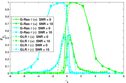
Figure 4: $P_{D_{0}}$ vs $\tau_{k}=\tau$, $P_{F_{0}}=0.01$; WSN with $K=49$ sensors, $P_{e,k}=0$, $\mathrm{SNR}\in\{0,10\}$ (amplitude signal with positive/negative polarity).

Secondly, in Fig. 5, we report $P_{D_{0}}$ (under $P_{F_{0}}=0.01$) versus target location $\bm{x}_{T}$ (for $\mathrm{SNR}=5\,\mathrm{dB}$), in order to obtain a clear comparison of detection performance over the entire surveillance area $\mathcal{A}$. It is apparent that the G-Rao test presents only marginal loss over the GLRT. By looking at the similar qualitative behaviour between Laplace and Gaussian noise (reported in the paper), we conclude that such trend is quite general for unimodal zero-mean noise pdfs.

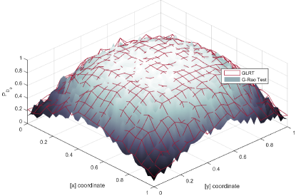
Figure 5: $P_{D_{0}}$ vs $\bm{x}_{T}$, $P_{F_{0}}=0.01$; WSN with $K=49$ sensors, $\tau_{k}=0$, $P_{e,k}=0$, $\mathrm{SNR=5\,\mathrm{dB}}$.

Finally, in Fig. 6 we compare the $P_{D_{0}}$ (for $P_{F_{0}}\in\{0.05,0.01\}$) of considered rules (for a target with randomly drawn position within $\mathcal{A}$) versus $\mathrm{SNR}$ ($\mathrm{dB}$), in order to obtain a comparison of detection sensitivity versus the signal strength. It is apparent that both rules perform very similarly over the whole SNR range, as well as for a different quality of the reporting channel ($P_{e,k}=P_{e}\in\{0,0.1\}$), with G-Rao slightly outperforming the GLRT at low SNR.

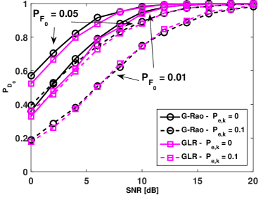
Figure 6: $P_{D_{0}}$ vs. $\mathrm{SNR}$ ($\mathrm{dB}$), $P_{F_{0}}\in\{0.05,0.01\}$; WSN with $K=49$ sensors, $\tau_{k}=0$, $P_{e,k}=P_{e}\in\{0,0.1\}$.

VI Conclusions

We developed a generalized version of the Rao test (G-Rao, based on [19]) for decentralized detection of a non-cooperative target emitting an unknown deterministic signal ($\theta$) at unknown location ($\bm{x}_{T}$), as an attractive (low-complexity) alternative to GLRT (the latter requiring a grid search on the whole space $(\theta,\bm{x}_{T})$) for a general model with quantized measurements, zero-mean, unimodal and symmetric noise (pdf), non-ideal and non-identical BSCs. Since $\bm{x}_{T}$ is a nuisance parameter present only under $\mathcal{H}_{1}$ (i.e. when $\theta\neq 0$), the G-Rao statistic arises from maximization (w.r.t. $\bm{x}_{T}$) of a family of Rao decision statistics, obtained by assuming $\bm{x}_{T}$ known. We also developed a reasonable criterion for optimized sensor thresholds: the zero choice was shown to be appealing for many pdfs of interest. This result was exploited to optimize the performance of G-Rao and GLR tests. Also, it was shown through simulations that the G-Rao test, achieves practically the same performance as the GLRT in the cases considered.

References

- [1] C.-Y. Chong and S. P. Kumar, “Sensor networks: evolution, opportunities, and challenges,” Proceedings of the IEEE, vol. 91, no. 8, pp. 1247–1256, 2003.
- [2] P. K. Varshney, Distributed Detection and Data Fusion, 1st ed. Springer-Verlag New York, Inc., 1996.
- [3] J. N. Tsitsiklis, “Decentralized detection,” Advances in Statistical Signal Processing, vol. 2, no. 2, pp. 297–344, 1993.
- [4] R. Viswanathan and P. K. Varshney, “Distributed detection with multiple sensors - Part I: Fundamentals,” Proc. IEEE, vol. 85, no. 1, pp. 54–63, Jan. 1997.
- [5] D. Ciuonzo, G. Papa, G. Romano, P. Salvo Rossi, and P. Willett, “One-bit decentralized detection with a Rao test for multisensor fusion,” IEEE Signal Process. Lett., vol. 20, no. 9, pp. 861–864, 2013.
- [6] J. Fang, Y. Liu, H. Li, and S. Li, “One-bit quantizer design for multisensor GLRT fusion,” IEEE Signal Process. Lett., vol. 20, no. 3, pp. 257–260, Mar. 2013.
- [7] D. Ciuonzo and P. Salvo Rossi, “Decision fusion with unknown sensor detection probability,” IEEE Signal Process. Lett., vol. 21, no. 2, pp. 208–212, Feb. 2014.
- [8] D. Ciuonzo, A. De Maio, and P. Salvo Rossi, “A systematic framework for composite hypothesis testing of independent Bernoulli trials,” IEEE Signal Process. Lett., vol. 22, no. 9, pp. 1249–1253, 2015.
- [9] V. A. Aalo and R. Viswanathan, “Multilevel quantisation and fusion scheme for the decentralised detection of an unknown signal,” Proc. of IEE Radar, Sonar and Navig., vol. 141, no. 1, pp. 37–44, Feb. 1994.
- [10] B. Chen, R. Jiang, T. Kasetkasem, and P. K. Varshney, “Channel aware decision fusion in wireless sensor networks,” IEEE Trans. Signal Process., vol. 52, no. 12, pp. 3454–3458, Dec. 2004.
- [11] R. Niu and P. K. Varshney, “Performance analysis of distributed detection in a random sensor field,” IEEE Trans. Signal Process., vol. 56, no. 1, pp. 339–349, Jan. 2008.
- [12] D. Ciuonzo, G. Romano, and P. Salvo Rossi, “Channel-aware decision fusion in distributed MIMO wireless sensor networks: Decode-and-fuse vs. decode-then-fuse,” IEEE Trans. Wireless Commun., vol. 11, no. 8, pp. 2976–2985, Aug. 2012.
- [13] D. Ciuonzo, G. Romano, and P. Salvo Rossi, “Optimality of received energy in decision fusion over Rayleigh fading diversity MAC with non-identical sensors,” IEEE Trans. Signal Process., vol. 61, no. 1, pp. 22–27, Jan. 2013.
- [14] S. M. Kay, Fundamentals of Statistical Signal Processing, Volume 2: Detection Theory. Prentice Hall PTR, Jan. 1998.
- [15] R. Niu and P. K. Varshney, “Joint detection and localization in sensor networks based on local decisions,” in 40th Asilomar Conference on Signals, Systems and Computers, 2006, pp. 525–529.
- [16] S. G. Iyengar, R. Niu, and P. K. Varshney, “Fusing dependent decisions for hypothesis testing with heterogeneous sensors,” IEEE Trans. Signal Process., vol. 60, no. 9, pp. 4888–4897, Sep. 2012.
- [17] A. Shoari and A. Seyedi, “Detection of a non-cooperative transmitter in Rayleigh fading with binary observations,” in IEEE Military Communications Conference (MILCOM), 2012, pp. 1–5.
- [18] D. Ciuonzo and P. Salvo Rossi, “Distributed detection of a non-cooperative target via generalized locally-optimum approaches,” Information Fusion, special issue on Event-Based Distributed Information Fusion Over Sensor Networks, vol. 36, pp. 261–274, Jul. 2017.
- [19] R. D. Davies, “Hypothesis testing when a nuisance parameter is present only under the alternative,” Biometrika, vol. 74, no. 1, pp. 33–43, 1987.
- [20] H. C. Papadopoulos, G. W. Wornell, and A. V. Oppenheim, “Sequential signal encoding from noisy measurements using quantizers with dynamic bias control,” IEEE Trans. Inf. Theory, vol. 47, no. 3, pp. 978–1002, Mar. 2001.
- [21] D. Rousseau, G. V. Anand, and F. Chapeau-Blondeau, “Nonlinear estimation from quantized signals: Quantizer optimization and stochastic resonance,” in Proc. 3rd Int. Symp. Physics in Signal and Image Processing, 2003, pp. 89–92.