Axioms in Model-based Planners

Abstract

Axioms can be used to model derived predicates in domain- independent planning models. Formulating models which use axioms can sometimes result in problems with much smaller search spaces and shorter plans than the original model. Previous work on axiom-aware planners focused solely on state-space search planners. We propose axiom-aware planners based on answer set programming and integer proramming. We evaluate them on PDDL domains with axioms and show that they can exploit additional expressivity of axioms.

1 Introduction

Currently, in the most commonly studied classical planning models, all changes to the world are the direct effects of some operator. However, it is possible to model some effects as indirect effects which can be inferred from a set of basic state variables. Such derived predicates can be expressed in modeling languages such as PDDL and formalisms such as SAS+ as axioms, which encode logical rules defining how the derived predicates follow from basic variables. Planners have supported various forms of derived predicates since relatively early systems (?; ?), and PDDL has supported axioms which specify derived predicates as a logic program with negation-as-failure semantics since version 2.2 (?)

Consider, for example, the well-known single-agent puzzle game Sokoban, in which the player pushes stones around in a maze. The goal is to push all the stones to their destinations. The standard PDDL formulation of Sokoban used in the International Planning Competition(IPC) consists of two kinds of operators, push and move. push lets the player push a box in one direction, while move moves the player into an unoccupied location.

? (?) proposed a new formulation of Sokoban with axioms and showed that this leads to a problem with a smaller search space and shorter plan (?). They remove the move operators entirely, and introduce axioms to check whether the player can reach a box to push it. The reformulated push operators now have a derived predicate reachable(loc) instead of at-player=loc as their precondition. The values of the derived predicates are determined by the following axioms:

1. reachable(loc) $\leftarrow$ at-player=loc

2. reachable(loc) $\leftarrow$ reachable(from), clear(loc), connected(from,loc)

Intuitively, the first axiom means that the current location of the player is reachable. The second axiom means a location next to a reachable location is also reachable. With axioms, the search space only has the transitions caused by push operators, resulting in smaller search space and shorter plan.

Previous work on derived predicates and axioms for planning has focused on the advantages with respect expressivity (compactness) of domain modeling using axioms, (?), as well as forward state-space search algorithms which are aware of axioms (?; ?; ?).

One class of approaches to planning translates planning problem instances to instances of other domain-independent modeling frameworks such as SAT (?) and Integer Programming (IP) (?). We refer to planners based on such translation-based approaches model-based planners. While previous work focused solely on axiom-aware state-space-based planners, to our knowledge, little or no work has been done on PDDL domains with axioms to evaluate model-based planners A standard approach to model-based planning is to translate a planning problem instance into a $k$-step SAT/IP/CSP model, where a feasible solution to the $k$-step model corresponds to a solution to the original planning instance with $n<k$ “steps”. To our knowledge, no previous work has evaluated axiom-aware, model-based approaches to planning.

We propose two axiom-aware model-based planners called ASPlan and IPlan, which are based on answer set programming (ASP) and integer programming (IP) respectively. Answer set programming (ASP) is a form of declarative programming based on answer set semantics of logic programming, and thus is a natural candidate for integrating axioms. Early attempts to apply ASP to planning (?) and (?) predated PDDL, and were not evaluated on large sets of benchmarks. To our knowledge, the first ASP-based planner compatible with PDDL is plasp (?). However, plasp does not handle axioms. We developed ASPlan based on plasp, but used the PDDL to SAS+ translator from FastDownward (?) to make it compatible with larger sets of IPC domains including domains with axioms. IPlan is an IP-based planner based on Optiplan (?). We integrated axioms into IPlan by using the ASP to IP translation method by (?).

To our knowledge, ASPlan and IPlan are the first model-based planners which handle axioms. We evaluate ASPlan and IPlan on an extensive set of benchmark domains with axioms, and show that additional expressivity of axioms benefit model-based planners as well. The rest of this paper is structured as follows. We first review background material including normal logic problems, SAS+ with axioms, and the search semantics for model-based planning (Section 2). Then, we describe ASPlan, our axiom-aware answer set programming based planner (Section 3) and IPlan, our axiom-aware, IP-based planner (Section 4). Section 5 presents our experimental evaluation of ASPlan and IPlan on an extensive set of domains with axioms, including IPC domains as well as domains used in previous work on planning with axiom-aware forward search planning (?; ?; ?). We conclude with a summary of our contributions (Section 6).

2 Preliminaries

2.1 Normal Logic Problem

We introduce normal logic problems, adopting the notations used in (?).

Definition 1.

A normal logic problem (NLP) $P$ consists of rules of the form

$$a\leftarrow b_{1},...,b_{m},{\rm not}c_{1},...,{\rm not}c_{n}.$$ (1)

where each $a$, $b_{i}$, $c_{j}$ is a ground atom.

Given a rule $r\in P$, we denote the head of rule $a$ by $H(r)$, the body $\{b_{1},...,b_{m},{\rm not}c_{1},...,{\rm not}c_{n}\}$ as $B(r)$, the positive body literals $\{b_{1},...,b_{m}\}$ as $B^{+}(r)$ and the negative body literals $\{{\rm not}c_{1},...,{\rm not}c_{n}\}$ as $B^{-}(r)$. We use $At(P)$ for the set of atoms which appear in $P$.

A set of atoms $M$ satisfies an atom $a$ if $a\in M$ and a negative literal ${\rm not}a$ if $a\not\in M$, denoted $M\vDash a$ and $M\vDash{\rm not}a$, respectively; $M$ satisfies a set of literals $L$, denoted $M\vDash L$, if it satisfies each literal in $L$; $M$ satisfies a rule $r$, denoted $M\vDash r$, if $M\vDash H(r)$ whenever $M\vDash B(r)$. A set of atoms $M$ is a model of $P$, denoted $M\vDash P$, if $M$ satisfies each rule of $P$.

An answer set of a program is defined through the concept of reduct.

Definition 2.

For a normal logic program $P$ and a set of atoms $M$, the reduct $P^{M}$ is defined as

$$P^{M}=\{H(r)\leftarrow B^{+}(r)\mid r\in P,B^{-}(r)\cap M=\emptyset\}.$$ (2)

Definition 3 (? ?).

A model $M$ of a normal logic program $P$ is an answer set iff $M$ is the minimal model of $P^{M}$.

Consider a program $P_{1}$ with the following rules:

$$(r_{1})\quad a \leftarrow{\rm not}b.$$ (3)

$$(r_{2})\quad b \leftarrow{\rm not}a.$$ (4)

$$(r_{3})\quad c \leftarrow a.$$ (5)

$M_{1}=\{a,c\}$ and $M_{2}=\{b\}$ are the answer sets of the program $P_{1}$ since they are the minimal model of $P_{1}^{M_{1}}$ and $P_{1}^{M_{2}}$ respectively.

We are particularly interested in locally stratified programs, which disallow negation through recursions (?).

Definition 4.

A normal logic program $P$ is locally stratified if and only if there is a mapping $l$ from $At(P)$ to $\{1,...,\lvert At(p)\rvert\}$ such that:

• for every rule $r$ with $H(r)=a$ and every $b\in B^{+}(r)$ , $l(b)\leq l(a)$

• for every rule $r$ with $H(r)=a$ and every $c\in C^{-}(r)$, $l(c)<l(a)$

Consider a program $P_{2}$ with the following rules:

$$(r_{4})\quad a \leftarrow{\rm not}b.$$ (6)

$$(r_{5})\quad b \leftarrow c.$$ (7)

$$(r_{6})\quad c \leftarrow b.$$ (8)

$P_{2}$ is locally stratified since there exists a mapping $l$ with $l(a)=2$ and $l(b)=l(c)=1$ satisfying Definition 4. Note that there is no mapping $l$ for $P_{1}$ due to the negative recursions through the rules $r_{1}$ and $r_{2}$.

With stratifications the unique model, called a perfect model can be computed by a stratified fixpoint procedure (?). It is known that the perfect model for a locally stratified program coincides with the unique answer set of the program (?). Indeed, $P_{2}$ has the unique model $M=\{a\}$.

2.2 SAS+ and Axioms

We adopt the definition of SAS+ or finite domain representation (FDR) used in ? (?) and ? (?).

Definition 5.

An SAS+ problem $\Pi$ is a tuple $(\allowbreak V\allowbreak,\allowbreak U\allowbreak,\allowbreak A\allowbreak,\allowbreak O,\allowbreak I,\allowbreak G\allowbreak)$ where

- $V$ is a set of primary variables. Each variable $v_{i}$ has a finite domain of values $D(v_{i})$.

- $U$ is a set of secondary variables. Secondary variables are binary and do not appear in operator effects. Their values are determined by axioms after each operator execution.

- $A$ is a set of rules of the form (1). Axioms and primary variables form a locally stratified logic program. At each state, axioms are evaluated to derive the values of secondary variables, resulting in an extended state. We denote the result of evaluating a set of axioms $A$ in a state $s$ as $A(s)$ and simply call it a state when there is no confusion. Note that $A(s)$ is guaranteed to be unique due to the uniqueness of the model for locally stratified logic programs.

- $O$ is a set of operators. Each operator $o$ has a precondition (pre($o$)), which consists of variable assignments of the form $v_{i}=x$ where $x\in D(v_{i})$. We abbreviate $v_{i}=1$ as $v_{i}$ when we know the variable is binary. An operator $o$ is applicable in a state $s$ iff $s$ satisfies pre($o$).

Each operator $o$ also has a set of effects (eff($o$)). Each effect $e\in$eff($o$) consists of a tuple (cond($e$), affected($e$)) where cond($e$) is a possibly empty variable assignment and affected($e$) is a single variable-value pair. Applying an operator $o$ with an effect $e$ to a state $s$ where cond($e$) is satisfied results in a state ($o(s)$) where affected($e$) is true. Although the original definition (?) does not specify this, we assume that conflicting effects, which assign different values to the same variable, never get triggered.

cost($o$) is the cost associated with the operator $o$.

- $I$ is an initial assignment over primary variables.

- $G$ is a partial assignment over variables that specifies the goal conditions.

A solution (plan) to $\Pi$ is an applicable sequence of operators $o_{0},...,o_{n}$ that maps $I$ into a state where $G$ holds.

2.3 $\forall$ vs. sequential ($seq$-) semantics

A standard, sequential search strategy for a model-based planner first generates a 1-step model (e.g., SAT/IP model), and attempts to solve it. If it has a solution, then the system terminates. Otherwise, a 2-step model is attempted, and so on (?). Adding axioms changes the semantics of a “step” in the $k$-step model. As noted by ? (?) and Rintanen et al (?), most model-based planners, including the base IPlan/ASPlan planners we evaluate below, use $\forall$ semantics, where each “step” in a $k$-step model consists of a set of operators which are independent of each other and can, therefore, be executed in parallel. In contrast, sequential semantics ($seq$-semantics) adds exactly 1 operator at each step in the iterative, sequential search strategy. In general, solving a problem using $\forall$ semantics is faster than with $seq$-semantics, since $\forall$ semantics significantly decreases the number of iterations of the sequential search strategy. For the domains with axioms, however, we add a constraint which restricts the number of operators executed at each step to 1, imposing $seq$-semantics. This is because a single operator can have far-reaching effects on derived variables, and establishing independence with respect to all derived variables affected by multiple operators is non-trivial.

3 ASPlan

We describe our answer set programming based planner ASPlan. ASPlan adapts the encoding of plasp (?) to the multi-valued semantics of SAS+. While plasp directly encodes PDDL to ASP, ASPlan first obtains the grounded SAS+ model from PDDL using the FastDownward translator, and then encodes the SAS+ to ASP. Using the FastDownward translator makes it easier to handle more advanced features like axioms and conditional effects.

3.1 Baseline Implementation

We translate a planning instance to an answer set program with $k$ steps. Having $k$-steps means that we have $k+1$ states or “layers” to consider. The notation here adheres to the ASP language standard.

const n = k. step 1..n. layer 0..n. (9)

For each $v_{i}=x\in I$, we introduce the following rule which specifies the initial state.

holds(f($$v_{i} x$$,),0) (10)

Likewise, for each $v_{i}=x\in G$, we have the following rule.

goal(f($$v_{i} x$$,)) (11)

The next rule (12) makes sure that all of the goals are satisfied at the last step.

$$\leftarrow$$ goal(F), not holds(F,n) (12)

For each operator $o\in O$ and each $v_{i}=x$ and $v_{j}=y$ in $o$’s preconditions and effects respectively, we introduce the following rules.

demands($$o v_{i} x o v_{j} y$$,f(,)). add(,f(,)). (13)

Rules (14) and (15) require that applied operators’ preconditions and effects must be realized.

$$\leftarrow$$ apply(O,T), demands(O,F), not holds(F,T-1), step(T). (14)

holds(F,T) $$\leftarrow$$ apply(O,T), add(O,F), step(T) (15)

Inertial axioms (unchanged variables retain their values) are represented by rules (16)-(17). An assignment $v=x$ to a SAS+ variable is mapped to an atom f($v$,$x$).

changed(X,T) $$\leftarrow$$ apply(O,T), add(O,f(X,Y)), step(T) (16)

$$\text{ holds(f(X,Y),T) $\leftarrow$ holds(f(X,Y),T-1), step(T),}\\ \text{inertial(f(X,Y)), not changed(X,T)}$$ (17)

Note that every primary variable $v$ is marked as inertial with the following rule.

inertial(f($$v val$$,)) (18)

With sequential semantics, rule (19) ensures that only one operator is applicable in each step.

1 {apply(O,T) : operators(O)} 1, step(T) (19)

On the other hand, with $\forall$-semantics, (20)-(22) requires that no conflicting operators are applicable at the same step.

1 {apply(O,T) : operators(O)}, step(T) (20)

$$\text{ $\leftarrow$ apply(O,T), apply(O',T), add(O,f(X,Y)),}\\ \text{ demands(O',f(X,Z)), step(T), O != O', Y != Z}$$ (21)

$$\text{ $\leftarrow$ apply(O,T), apply(O',T), add(O,f(X,Y)),}\\ \text{ add(O',f(X,Z)), step(T), O != O', Y != Z.}$$ (22)

Since variables in SAS+ cannot take different values at the same time, we introduce the mutex constraint (23). A mutex is a set of fluents of which at most one is true in every state.

$$\leftarrow$$ holds(f(X,Y),T), holds(f(X,Z),T), Y != Z, layer(T). (23)

3.2 Integrating Axioms

Integrating axioms to ASPlan is fairly straightforward. For an axiom $a\leftarrow b_{1},...,b_{n},notc_{1},...,c_{m}$, we introduce the following rule:

$$\text{ holds(f($a$,1),T) $\leftarrow$ holds(f($b_{1}$,1),T),...,holds(f($b_{n}$,1),T),}\\ \text{ not holds(f($c_{1}$,0),T),..., not holds(f($c_{m}$,0),T), step(T).}$$ (24)

We also need the following constraints to realize negation-as-failure semantics while being compatible with the formulations above.

holds(f($$u \leftarrow u$$,0),T) not holds(f(,1),T), layer(T). (25)

$$\leftarrow u u$$ not holds(f(,0),T), not holds(f(,1),T), layer(T). (26)

3.3 Integrating Conditional Effects

We describe how to integrate conditional effects into ASPlan. For each operator $o$ and its effect $e\in$eff($o$), we introduce the following rule

$$\text{ fired(E,T) $\leftarrow$ apply(A,T),}\\ \text{ holds(f($v_{1}$,$x$),T), ..., holds(f($v_{n}$,$z$),T), step(T)}$$ (27)

where $v_{1}=x$,…,$v_{n}=z$ are in cond($e$).

With conditional effects, applying operators does not necessarily mean their effects get triggered. We replace rules (15) and (16) with the following rules.

holds(F,T) $$\leftarrow$$ fired(E,T), add(E,F), effect(E), step(T) (28)

changed(X,T) $$\leftarrow$$ fired(E,T), add(E,f(X,Y)), effect(E), step(T) (29)

4 IPlan

4.1 Baseline Implementation

We describe our baseline integer-programming planner IPlan, which is based on Optiplan (?). Optiplan, in turn, extends the state-change variable model (?), and the Optiplan model is defined for an propositional (STRIPS) framework. IPlan adapts the Optiplan model for the multi-valued SAS+ framework, exploiting the FastDownward translator (?).

An assignment $v=x$ to a SAS+ variable is mapped to a fluent $f$. For all fluents $f$ and time step $t$, Optiplan has the following binary state change variables. $pre_{f}$, $add_{f}$ and $del_{f}$ denote a set of operators that might require, add, or delete $f$ respectively. Intuitively, state change variables represent all possible changes of fluents at time step $t$.

• ${x^{maintain}_{f,t}}=1\text{ iff fluent }f\text{ is propagated in step }t$

• ${x^{preadd}_{f,t}}=1\text{ iff }o\in pre_{f}\setminus del_{f}\text{ is executed in step }t$

• ${x^{predel}_{f,t}}=1\text{ iff }o\in pre_{f}\cap del_{f}\text{ is executed in step }t$

• ${x^{add}_{f,t}}=1\text{ iff }o\in add_{f}\setminus pre_{f}\text{ is executed in step }t$

• ${x^{del}_{f,t}}=1\text{ iff }o\in del_{f}\setminus pre_{f}\text{ is executed in step }t$

For all operators $o$ and time step $t$, Optiplan has the binary operator variables.

$${y_{o,t}}=1\text{iff operator }o\text{ is executed in period }t$$

Constraints (30) and (31) represent the initial states constraints.

$${x^{add}_{f,0}} =1\quad\forall f\in I$$ (30)

$${x^{add}_{f,0}},{x^{maintain}_{f,0}},{x^{preadd}_{f,0}} =0\quad\forall f\not\in I$$ (31)

Constraint (32) ensures that the goals are satisfied at the last step $T$ (${x^{sat}_{f,t}}$ is introduced later).

$${x^{sat}_{f,t}}\geq 1\quad\forall f\in G,t=T$$ (32)

For all fluents $f$ and time step $t$, Optiplan has the following constraints to make sure the state change variables have the intended semantics.

$$\sum_{o\in add_{f}\setminus pre_{f}}{y_{o,t}} \geq{x^{add}_{f,t}}$$ (33)

$${y_{o,t}} \leq{x^{add}_{f,t}}\quad\forall o\in add_{f}\setminus pre_{f}$$ (34)

$$\sum_{o\in del_{f}\setminus pre_{f}}{y_{o,t}} \geq{x^{del}_{f,t}}$$ (35)

$${y_{o,t}} \leq{x^{del}_{f,t}}\quad\forall o\in del_{f}\setminus pre_{f}$$ (36)

$$\sum_{o\in pre_{f}\setminus del_{f}}{y_{o,t}} \geq{x^{preadd}_{f,t}}$$ (37)

$${y_{o,t}} \leq{x^{preadd}_{f,t}}\quad\forall o\in pre_{f}\setminus del_{f}$$ (38)

$$\sum_{o\in pre_{f}\cap del_{f}}{y_{o,t}} ={x^{predel}_{f,t}}$$ (39)

Constraints (40) and (41) restrict certain state changes from occurring in parallel.

$${x^{add}_{f,t}}+{x^{maintain}_{f,t}}+{x^{del}_{f,t}}+{x^{predel}_{f,t}} \leq 1$$ (40)

$${x^{preadd}_{f,t}}+{x^{maintain}_{f,t}}+{x^{del}_{f,t}}+{x^{predel}_{f,t}} \leq 1$$ (41)

Constraint (42) represents the backward chaining requirement, that is, if a fluent $f$ is true at the beginning of step $t$ then there must have been a change that made $f$ true at step $t-1$, or it was already true at $t-1$ and maintained.

$${x^{preadd}_{f,t}}+{x^{maintain}_{f,t}}+{x^{predel}_{f,t}}\leq\\ {x^{preadd}_{f,t-1}}+{x^{add}_{f,t-1}}+{x^{maintain}_{f,t-1}}\quad\forall f\in F,t\in 1,...,T$$ (42)

New Mutex Constraints

IPlan augments the Optiplan model with a new set of mutex constraints. In addition to the above variables and constraints which are from Optiplan, IPlan introduces a set of auxiliary binary variables ${x^{sat}_{f,t}}$, which correspond to the value of the fluent $f$ at the time step $t$ and are constrained as follows.

$${x^{sat}_{f,t}}\leq{x^{add}_{f,t}}+{x^{preadd}_{f,t}}+{x^{maintain}_{f,t}}$$ (43)

$${x^{sat}_{f,t}}\geq{x^{add}_{f,t}}$$ (44)

$${x^{sat}_{f,t}}\geq{x^{preadd}_{f,t}}$$ (45)

$${x^{sat}_{f,t}}\geq{x^{maintain}_{f,t}}$$ (46)

Using ${x^{sat}_{f,t}}$, mutex constraints can be implemented as follows. For every mutex group $g$ (at most one fluent in $g$ can be true at the same time) found by the FastDownward (?) translator, IPlan adds the following constraint.

$$\sum_{f\in g}{x^{sat}_{f,t}}\leq 1$$ (47)

? (?) used similar mutex constraints for thier CP-based planner.

4.2 Integrating Axioms

We describe how to integrate axioms into an IP-based model. For each time step $t$, axioms form the corresponding normal logic program (NLP) $P_{t}$. The models for $P_{t}$ correspond to the truth values for the derived variables. We translate each NLP $P_{t}$ to an integer program (IP) using the method by ? (?), and add these linear constraints to the IPlan model.

Level Rankings

Translation from a NLP to an IP by ? (?) relies on characterizing answer sets using level rankings. Intuitively, a level ranking of a set of atoms gives an order in which the atoms are derived.

Definition 6 (? ?).

Let $M$ be a set of atoms and $P$ a normal program. A function $lr:M\rightarrow N$ is a level ranking of $M$ for $P$ iff for each $a\in M$, there is a rule $r\in P_{M}$ such that $H(r)=a$ and for every $b\in B^{+}(r)$, $lr(a)-1\geq lr(b)$.

Note that $P_{M}$ is the set of support rules, which are essentially the rules applicable under $M$.

Definition 7 (? ?).

For a program $P$ and $I\subset At(P)$, $P_{I}=\{r\in P\mid I\vDash B(r)\}$ is the set of support rules.

The level ranking characterization gives the condition under which a supported model is an answer set.

Definition 8 (? ?).

A set of atoms $M$ is a supported model of a program $P$ iff $M\vDash P$ and for every atom $a\in M$ there is a rule $r\in P$ such that $H(r)=a$ and $M\vDash B(r)$.

Theorem 1 (? ?).

Let $M$ be a supported model of a normal program $P$. Then $M$ is an answer set of $P$ iff there is a level ranking of $M$ for $P$.

Consider, for example, program $P_{2}$ (from Section 2.1) and its model $M^{\prime}=\{b,c\}$. $M^{\prime}$ is a supported model for $P_{2}$ satisfying the Definition 8. $M^{\prime}$, however, is not an answer set of $P_{2}$ since there is no level ranking for $M^{\prime}$ with the atoms $b$ and $c$ forming a cycle.

Components and Defining Rules

? (?) define a dependency graph of a normal logic program to be used for the translation to IP.

Definition 9 (? ?).

The dependency graph of a program $P$ is a directed graph $G$ = $\langle V,E\rangle$ where $V$ = $At(P)$ and $E$ is a set of edges $\langle a,b\rangle$ for which there is a rule $r\in P$ such that $H(r)$ = $a$ and $b\in B^{+}(r)$.

For example, the dependency graph for $P_{2}$ is shown in Figure 1. We use SCC($a$) to denote the strongly connected component (SCC) containing an atom $a$.

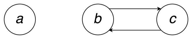
Figure 1: The dependency graph for $P_{2}$.

Definition 10 (? ?).

For a program $P$ and an atom $a\in At(P)$, respective sets of defining rules, externally defining rules, and internally defining rules are defined as follows:

$${\rm Def}_{P}(a)=\{r\in P\mid H(r)=a\}$$ (48)

$${\rm Ext}_{P}(a)=\{r\in{\rm Def}_{P}(a)\mid B^{+}(r)\cap{\rm SCC}(a)=\emptyset\}$$ (49)

$${\rm Int}_{P}(a)=\{r\in{\rm Def}_{P}(a)\mid B^{+}(r)\cap{\rm SCC}(a)\neq\emptyset\}$$ (50)

The set of internally supporting atoms is defined as

$${\rm IS}(a,r)={\rm SCC}(a)\cap B^{+}(r).$$ (51)

For example, for $P_{2}$, ${\rm Def}_{P_{2}}(a)={\rm Ext}_{P_{2}}(a)=\{r_{4}\}$, ${\rm Def}_{P_{2}}(b)={\rm Int}_{P_{2}}(b)=\{r_{5}\}$ and ${\rm Def}_{P_{2}}(c)={\rm Int}_{P_{2}}(c)=\{r_{6}\}$.

Translation

We are now ready to describe how to translate a normal logic program $P_{t}$ formed by axioms to linear constraints based on the method by ? (?). The translation consists of linear constraints developed below.

1. For each secondary variable $u\in U$, introduce a binary variable ${x^{sat}_{u,t}}$.

2. For each secondary variable $u\in U$, include the following constraint

   $$\sum_{r\in{{\rm Def}_{P}(u)}}bd^{r}_{t}-|{{\rm Def}_{P}(u)}|\cdot{x^{sat}_{u,t}}\leq 0$$ (52)

   where $bd^{r}_{t}$ is a binary variable for each $r\in{{\rm Def}_{P}(u)}$ and step $t$. Intuitively, $bd^{r}_{t}$ represents whether the body of $r$ is satisfied at step $t$. The constraint ensures that when one of the rules defining $u$ (${{\rm Def}_{P}(u)}$) is satisfied, ${x^{sat}_{u,t}}$ must be true (${x^{sat}_{u,t}}=1$). For example, for atom $a$ in $P_{2}$, this introduces the constraint $bd^{r_{4}}_{t}-1\cdot{x^{sat}_{a,t}}\leq 0$.

3. For each axiom $r\in A$, include the following constraints.

   $$\sum_{b\in B^{+}(r)}{x^{sat}_{b,t}}-\sum_{c\in B^{-}(r)}{x^{sat}_{c,t}}-|B(r)|\cdot bd^{r}_{t}\geq-|B^{-}(r)|$$ (53)

   $$\sum_{b\in B^{+}(r)}{x^{sat}_{b,t}}-\sum_{c\in B^{-}(r)}{x^{sat}_{c,t}}-bd^{r}_{t}\leq|B^{+}(r)|-1$$ (54)

   Constraints (53) and (54) express the fact that the body of rule $r$ is satisfied iff each literal in $B(r)$ is satisfied. For example, for $r_{6}$ in $P_{2}$, this introduces the constraints ${x^{sat}_{b,t}}-1\cdot bd^{r_{6}}\geq-0$ and ${x^{sat}_{b,t}}-bd^{r_{6}}_{t}\leq 1-1$.

4. For each secondary variable $u\in U$, include the constraint

   $$\sum_{r\in{{\rm Ext}_{P}(u)}}bd^{r}_{t}+\sum_{r\in{{\rm Int}_{P}(u)}}s^{r}_{t}-{x^{sat}_{u,t}}\geq 0$$ (55)

   where $s^{r}_{t}$ is a binary variable for each $r\in{{\rm Int}_{P}(u)}$ and each step $t$. Intuitively, the binary variable $s^{r}_{t}$ represents whether the respective ranking constraints for the rule $r$ are satisfied in addition to its body. The constraint requires ${x^{sat}_{u,t}}$ to be true when one of its externally defining rules is satisfied or one of its internally defining rules is satisfied while respecting the ranking constraints. For example, for atom $a$ and $c$ in $P_{2}$, this introduces the constraints $bd^{r_{4}}_{t}+0-{x^{sat}_{a,t}}\geq 0$ and $0+s^{r_{6}}_{t}-{x^{sat}_{c,t}}\geq 0$ respectively.

5. For each secondary variable $u\in U$ and each $r\in{{\rm Int}_{P}(u)}$, include the constraints

   $$bd^{r}_{t}-s^{r}_{t}\geq 0$$ (56)

   $$\sum_{b(b\in{{\rm IS}(u,r)})}gt^{ub}_{t}-|{{\rm IS}(u,r)}|\cdot s^{r}_{t}\geq 0$$ (57)

   where $gt^{ub}_{t}$ is a binary variable for each $b\in{{\rm IS}(u,r)}$, which represents whether the rank of $u$ is greater than that of $b$. For example, for atom $c$ and $r_{6}$ in $P_{2}$, this introduces the constraints $gt^{cb}_{5}-1\cdot s^{r_{6}}_{5}\geq 0$.

6. For each secondary variable $u\in U$ and each $r\in{{\rm Int}_{P}(u)}$, and each $b\in{{\rm IS}(u,r)}$, include the constraint

   $$z_{a,t}-z_{b,t}-|{{\rm SCC}(u)}|\cdot gt^{ab}_{t}\geq 1-|{{\rm SCC}(u)}|$$ (58)

   where $z_{a,t}$ and $z_{b,t}$ are integer variables representing level rankings for $a$ and $b$ respectively. Constraint (58) guarantees that if $gt^{ab}_{t}=1$ then $z_{a,t}\geq z_{b,t}$. e.g., for atom $c$ in $P_{2}$, this introduces the constraint $z_{c,t}-z_{b,t}-2\cdot gt^{cb}_{t}\geq 1-2$.

In the above constraints, ${x^{sat}_{u,t}}$ corresponds to the values of a secondary variable $u$ at time step $t$. Since secondary variables only appear in operator preconditions, we only need to make sure the preconditions of applied operators are satisfied.

$$y_{u,t}\leq{x^{sat}_{u,t}}\quad\forall a\in pre_{f}\setminus del_{f}$$ (59)

As explained in Section 2.3 , in case of domains with axioms, we need to add the following constraint to restrict the number of operators executed at each time step to 1.

$$\sum y_{a,t}\leq 1$$ (60)

5 Experimental Results

All experiments are performed on a Xeon E5-2670 v3, 2.3GHz with 2GB RAM and 5 minute time limit. In all experiments, the runtime limits include all steps of problem solving, including translation/parsing, and search. We use clingo4.5.4, a state-of-the-art ASP solver (?) to solve the ASP models produced by ASPlan. The IP models produced by IPlan are solved using Gurobi Optimizer 6.5.0, single-threaded.

The rules and constraints used in each of our planner configurations are summarized in Table 1.

5.1 Baseline Evaluation on PDDL Domains without Axioms

We first evaluated ASPlanS and IPlanS on PDDL domains without axioms to compare them against existing planners. A thorough comparison of model-based planners is non-trivial because of the multitude of combinations possible of translation schemes, solvers, and search strategies. The purpose of this experiment is to show that the baseline ASPlan and IPlan planners perform reasonably well compared to similar, existing model-based planners which (1) use a simple search strategy which iteratively solves $k$-step models, and (2) use models which are solved by “off-the-shelf” solver algorithms, i.e., this excludes planners that such as Madagascar (?), which uses a more sophisticated search strategy and customized solver algorithm, as well as the flow-based IP approaches (?).

We compared the following: (1) plasp (2) APlanS (ASPlan with seq-semantics) (3) IPlanS (IPlan with seq-semantics) (4) ASPlan (ASPlan with $\forall$-semantics) (5) IPlan (IPlan with $\forall$-semantics) (6) SCV (IPlan without the mutex constraints) (7) TCPP, a state of the art CSP-based planner (?).

We used plasp with the default configurations with sequential semantics. Since plasp uses incremental grounding, we used iClingo (?) as an underlying solver. Note that ASPlan could have used incremental grounding as well, but we decided not to for ease of implementation. As for TCPP, we could not obtain the souce code from the authors as of this writing, so we use the results from the original paper. We chose the overall-best-performing configuration TCPPxm-conf-sac, which uses don’t care and mutex constraints proposed in (?). The results are shown in Table 2.

ASPlanS dominated plasp in every domain, indicating that ASPlan is a reasonable, baseline ASP-based solver. This is to be expected, since ASPlanS is based on the plasp model while utilizing FastDownward tranlator for operator grounding, although ASPlans does not use incremental grounding. Among $\forall$-semantics solvers ASPlan, IPlan and TCPP, ASPlan and IPlan are highly competitive with TCPP despite the fact that the results for TCPP were obtained with a significantly longer (60min. vs. 5min) runtime limit (on a different machine). Comparing IPlan and SCV, additional mutex constraints increased coverage in domains such as blocks and logistics00.

ASPlan	ASPlanS	IPlan	IPlanS
(9)-(18) ,(20)-(23)	(9)-(19) ,(23)-(29)	(30)-(47)	(30)-(60)

Table 1: Summary of the rules or constraints used in each planner configuration

	#	plasp	ASPlanS	IPlanS	ASPlan	IPlan	SCV	TCPP
blocks	35	15	18	28	18	28	16	32
depot	22	2	2	2	9	11	7	11
driverlog	20	4	7	4	14	11	11	13
grid	5	1	2	1	0	1	0	2
gripper	20	2	2	2	3	4	4	2
freecell	80	6	7	7	1	18	18	4
logistics-98	35	2	2	1	12	16	11	9
logistics00	28	7	7	6	28	28	22	24
movie	30	30	30	30	30	30	30	N/A
mprime	35	24	27	21	11	25	24	26
mystery	30	16	16	13	9	16	13	17
rovers	40	0	4	4	23	21	18	22
satellite	36	3	4	5	11	8	8	7
zenotravel	20	6	7	3	13	13	11	12

Table 2: Results on domains without axioms with 2GB, 5min limits. For TCPP, the results from (?) on a Intel Xeon 2.60GHz CPU, 4GB, 60 min limit. are shown. N/A indicates a lack of the results. # denotes the number of instances for each domain.

5.2 Evaluation on PDDL Domains with Axioms

We evaluated ASPlan and IPlan on PDDL domains with axioms.

Below, we describe the domains (other than the previously described Sokoban) used in experimental evaluations,

Verification Domains

? (?) proposed a modeling formalism for capturing high level functional specifications and requirements of reactive control systems. The formulation consists of two agents, namely the environment which disturbs the system, and the controller, which tries to return the system to a safe state. If there is a sequence of operators for the environment that leads to an unsafe state, the control system has a vulnerability. We used two compiled versions of the formulation: (a) compilation into STRIPS (?), and (b) compilation into STRIPS with axioms (?).

ACC is a verification domain for Adaptive Cruise Control (ACC), a well known driver assistance feature present in many high end automotive system which is designed to take away the burden of adjusting the speed of the vehicle from the driver, mostly under light traffic conditions.

The GRID domain is a synthetic planning domain loosely based on cellular automata and incorporates a parallel depth first search protocol for added variety. Note that this domain is completely different from the standard IPC grid domain. To avoid confusion, we denote this verification domain as GRID-VERIFICATION.

Multi-Agent Domains

? (?) proposed a framework for handling beliefs in multiagent settings, building on the methods for representing beliefs for a single agent. Computing linear multiagent plans for the framework can be mapped to a classical planning problem with axioms. We use three of their domains.

Muddy Children, originally from ? (?), is a puzzle in which $k$ out of $n$ children have mud on their foreheads. Each child can see the other children’s foreheads but not their own. The goal for a child is to know if he or she has mud by sensing the beliefs of the others. Muddy Child is a reformulation of Muddy Children.

In Collaboration through Communication, the goal for an agent is to know a particular block’s location. Two agents volunteer information to each other to accomplish a task faster than that would be possible individually.

In Sum, there are three agents, each with a number on their forehead. It is known that one of the numbers equals the sum of the other two. The goal is for one or two selected agents to know their numbers.

Wordrooms is a variant of Collaboration through Communication where two agents must find out a hidden word from a list of n possible words.

PROMELA

This is a standard IPC-4 benchmarks domain with axioms (both the version with axioms as well as the compiled version without axioms were provided in the IPC-4 benchmark set). The task is to validate properties in systems of communicating processes (often communication protocols), encoded in the Promela language. ? (?) developed an automatic translation from Promela into PDDL, which was extended to generate the IPC domains. We used the IPC-4 benchmarks for the Dining Philosophers problem (philosophers), and the Optical Telegraph protocol (optical-telegraph).

PSR

The task of PSR (power supply restoration) is to reconfigure a faulty power distribution network so as to resupply customers affected by the faults. The network consists of electronic lines connected by switched and power sources with circuit breaker. PSR was modeled as a planning problem in ? (?). We used the version of PSR used in IPC-4, which is a simplified version of ? (?) with full observability of the world and no numeric optimization.

2GB, 5min	#	ASPlanS	IPlanS	Axioms
Domains from ? (?)
sokoban-axioms	30	5	4	Y
sokoban-opt08-strips	30	4	0	N
trapping_game	7	4	N/A	Y
Domains from ? (?)
acc-compiled	8	0	0	N
acc	8	7	1	Y
door-fixed	2	1	1	Y
door-broken	2	0	0	Y
grid-verification	99	0	0	Y
Domains from ? (?)
muddy-child-kg	7	1	N/A	Y
muddy-children-kg	5	1	N/A	Y
collab-and-comm-kg	3	1	N/A	Y
wordrooms-kg	5	1	N/A	Y
Domains from IPC
psr-middle	50	48	N/A	Y
psr-middle-noce	50	43	25	Y
psr-middle-compiled	50	1	N/A	N
psr-large	50	21	N/A	Y
optical-telegraphs	48	0	N/A	Y
optical-telegraphs-compiled	48	0	N/A	N
philosophers	48	2	N/A	Y
philosophers-compiled	48	1	N/A	N
miconic	150	29	25	N
miconic-axioms	150	40	61	Y
grid	5	2	0	N
grid-axioms	5	3	2	Y

Table 3: Results on domains with axioms. N/A indicates a lack of results since the current implementation of IPlan is not compatible with conditional effects. # denotes the number of instances for each domain. The ”Axioms” column indicates whether the corresponding domain has axioms

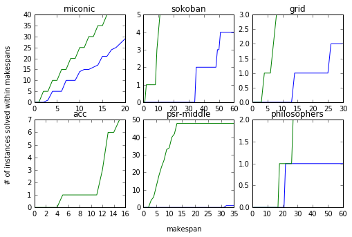
Figure 2: ASPlanS results showing the number of instances solved within makespan iterations (steps). The green lines represent domains with axioms, while the blue lines represent domains without axioms. Note that there can be instances which have solutions within a makespan but were not solved due to our time and memory limits.

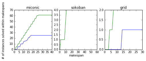
Figure 3: IPlanS results showing the number of instances solved within makespan iterations (steps). The green lines represent domains with axioms, while the blue lines represent domains without axioms. Note that there can be instances which have solutions within a makespan but were not solved due to our time and memory limits.

Grid and Miconic

Like Sokoban some of the domains from existing IPC benchmarks without axioms can be reformulated to domains with axioms. We chose grid and miconic from such domains for experimental evaluation.

In the grid domain, the player walks around a maze to retrieve the key to the goal. Just as in Sokoban the operators for the player’s movement can be replaced with reachability axioms. Operators for retrieving keys or unlocking doors now have new reachability variables as their preconditions.

miconic is an elevator domain where we must transport a set of passengers from their start floors to their destination floors. The up and down movements of an elevator can be expressed as axioms.

Note that in Sokoban, where move operators are zero cost, an optimal plan for an instance with axioms corresponds to an optimal plan for the original instance without axioms. In grid and miconic, however, this no longer holds since the operators expressed as axioms have positive costs.

Results

The coverage results are shown in Table 3. In addition, Figures 2-3 show the number of instances solved within makespan iterations (steps).

In Sokoban, acc, psr-middle, miconic, grid and philosophers ASPlan (and sometimes IPlan) solved more instances from the formulations with axioms than the compiled formulations without axioms. This is because compiled instances tend to have longer makespans (as shown in Figure 2 and 3), which tends to increase difficulty for model-based planners such as ASPlan and IPlan, because (1) the number of variables increases with makespan, and (2) in the iterative scheme used by model-basd planners (i.e., generating and attempting to solve $k$-step models with iteratively increasing $k$), problems with longer makespans increase the number of iterations which must be executed to find a plan.

6 Conclusion

We investigated the integration of PDDL derived predicates (axioms) into model-based planners. We proposed axiom-aware model-based planners ASPlan and IPlan. ASPlan is an ASP-based planner, which is able to handle axioms and conditional effects. IPlan is an IP-based planner based on Optiplan (?). We integrated axioms into IPlan using the ASP to IP translation method by (?). We evaluated ASPlan and IPlan on PDDL domains with axioms and showed that axiom-aware model-based planners can benefit from the fact that formulations with axioms tend to have shorter makespans than formulations of the same problem without axioms, resulting in higher coverage on the formulations with axioms.

References

- [Apt, Blair, and Walker 1988] Apt, K. R.; Blair, H. A.; and Walker, A. 1988. Towards a theory of declarative knowledge. Foundations of Deductive Databases and Logic Programming 89–148.
- [Barrett et al. 1995] Barrett, A.; Christianson, D.; Friedman, M.; Kwok, C.; Golden, K.; Penberthy, S.; Sun, Y.; and Weld, D. 1995. UCPOP users manual. Technical Report TR93-09-06d, University of Washington, CS Department.
- [Bonet, Thiébaux, and others 2003] Bonet, B.; Thiébaux, S.; et al. 2003. GPT meets PSR. In Proc. ICAPS, 102–112.
- [Coles and Smith 2007] Coles, A., and Smith, A. 2007. Marvin: A heuristic search planner with online macro-action learning. Journal of Artificial Intelligence Research 28:119–156.
- [Dimopoulos, Nebel, and Koehler 1997] Dimopoulos, Y.; Nebel, B.; and Koehler, J. 1997. Encoding planning problems in nonmonotonic logic programs. In Proc. European Conf. on Planning (ECP), 169–181.
- [Edelkamp and Hoffmann. 2004] Edelkamp, S., and Hoffmann., J. 2004. PDDL2.2: The language for the classical part of the 4th International Planning competition. Technical Report 195, Albert-Ludwigs-Universität Freiburg, Institut für Informatik, 2004.
- [Edelkamp 2003] Edelkamp, S. 2003. Promela planning. In Proceedings of the 10th Int. Conf. on Model checking software, 197–213.
- [Eiter, Ianni, and Krennwallner 2009] Eiter, T.; Ianni, G.; and Krennwallner, T. 2009. Answer set programming: A primer. In Reasoning Web. Semantic Technologies for Information Systems. Springer. 40–110.
- [Fagin et al. 2004] Fagin, R.; Halpern, J. Y.; Moses, Y.; and Vardi, M. 2004. Reasoning about knowledge. MIT press.
- [Gebser et al. 2008] Gebser, M.; Kaminski, R.; Kaufmann, B.; Ostrowski, M.; Schaub, T.; and Thiele, S. 2008. Engineering an incremental ASP solver. In Proc. ICLP, 190–205.
- [Gebser, Kaufmann, and Schaub 2012] Gebser, M.; Kaufmann, R.; and Schaub, T. 2012. Gearing up for effective ASP planning. In Correct Reasoning. Springer. 296–310.
- [Gelfond and Lifschitz 1988] Gelfond, M., and Lifschitz, V. 1988. The stable model semantics for logic programming. In Proc. ICLP, volume 88, 1070–1080.
- [Gerevini, Saetti, and Serina 2011] Gerevini, A.; Saetti, A.; and Serina, I. 2011. Planning in domains with derived predicates through rule-action graphs and local search. Annals of Mathematics and Artificial Intelligence 62(3-4):259–298.
- [Ghooshchi et al. 2017] Ghooshchi, N. G.; Namazi, M.; Newton, M. A. H.; and Sattar, A. 2017. Encoding domain transitions for constraint-based planning. Journal of Artificial Intelligence Research 58:905–966.
- [Ghosh, Dasgupta, and Ramesh 2015] Ghosh, K.; Dasgupta, P.; and Ramesh, S. 2015. Automated planning as an early verification tool for distributed control. Journal of Automated Reasoning 54(1):31–68.
- [Helmert 2006] Helmert, M. 2006. The Fast Downward planning system. Journal of Artificial Intelligence Research 26:191–246.
- [Helmert 2009] Helmert, M. 2009. Concise finite-domain representations for PDDL planning tasks. Artificial Intelligence 173(5):503–535.
- [Horie 2015] Horie, S. 2015. On model-based domain-independent planning. Undergraduate Thesis, University of Tokyo (in Japanese).
- [Ivankovic and Haslum 2015a] Ivankovic, F., and Haslum, P. 2015a. Code supplement for ”optimal planning with axioms. http://users.cecs.anu.edu.au/~patrik/tmp/fd-axiom-aware.tar.gz.
- [Ivankovic and Haslum 2015b] Ivankovic, F., and Haslum, P. 2015b. Optimal planning with axioms. In Proc. IJCAI, 1580–1586.
- [Kautz and Selman 1992] Kautz, H., and Selman, B. 1992. Planning as satisfiability. In Proc. ECAI, 359–363.
- [Kominis and Geffner 2015] Kominis, F., and Geffner, H. 2015. Beliefs in multiagent planning: From one agent to many. In Proc. ICAPS, 147–155.
- [Liu, Janhunen, and Niemeiä 2012] Liu, G.; Janhunen, T.; and Niemeiä, I. 2012. Answer set programming via mixed integer programming. In Proc. KR, 32–42.
- [Manna and Waldinger 1987] Manna, Z., and Waldinger, R. J. 1987. How to clear a block: A theory of plans. Journal of Automated Reasoning 3(4):343–377.
- [Niemelä 2008] Niemelä, I. 2008. Stable models and difference logic. Annals of Mathematics and Artificial Intelligence 53(1-4):313–329.
- [Potassco 2016] Potassco. 2016. The University of Potsdam Answer Set Programming collection (Potassco). http://potassco.sourceforge.net/.
- [Przymusinski 1988] Przymusinski, T. C. 1988. On the declarative semantics of deductive databases and logic programs. In Foundations of Deductive Databases and Logic Programming.
- [Rintanen, Heljanko, and Niemelä 2006] Rintanen, J.; Heljanko, K.; and Niemelä, I. 2006. Planning as satisfiability: parallel plans and algorithms for plan search. Aritificial Intelligence 170(12-13):1031–1080.
- [Subrahmanian and Zaniolo 1995] Subrahmanian, V., and Zaniolo, C. 1995. Relating stable models and ai planning domains. In Proc. ICLP, 233–247.
- [Thiébaux, Hoffmann, and Nebel 2005] Thiébaux, S.; Hoffmann, J.; and Nebel, B. 2005. In defense of PDDL axioms. Artificial Intelligence 168(1):38–69.
- [van den Briel and Kambhampati 2005] van den Briel, M. H. L., and Kambhampati, S. 2005. Optiplan: Unifying ip-based and graph-based planning. Journal of Artificial Intelligence Research 24(1):919–931.
- [van den Briel, Vossen, and Kambhampati 2008] van den Briel, M. H. L.; Vossen, T.; and Kambhampati, S. 2008. Loosely coupled formulations for automated planning: An integer programming perspective. Journal of Artificial Intelligence Research 31:217–257.
- [Vossen et al. 1999] Vossen, T.; Ball, M. O.; Lotem, A.; and Nau, D. S. 1999. On the use of integer programming models in AI planning. In Proc. IJCAI, 304–309.