Spin-orbit interaction driven dimerization in one dimensional frustrated magnets

Abstract

We study the effect of spin-orbit interaction on one-dimensional U(1)-invariant frustrated magnets with dominant critical nematic fluctuations. The spin-orbit coupling explicitly breaks the U(1) symmetry of arbitrary global spin rotations about the high-symmetry axis down to $Z_{2}$ (invariance under a $\pi$-rotation). Given that the nematic order parameter is invariant under a $\pi$-rotation, it is relevant to ask if other discrete symmetries can be spontaneously broken. Here we demonstrate that the spin-orbit coupling induces a bond density wave that spontaneously breaks the translational symmetry and opens a gap in the excitation spectrum.

I Introduction

Frustrated magnetism is a continuous source of exotic states of matter that challenge the existing characterization probes ref:review1 ; ref:review2 . Once quantum fluctuations melt the traditional magnetic long-range order, it often happens that the remaining liquid or multipolar orderings do not couple directly to the usual experimental probes. A simple example is the spin nematic phase proposed to be the ground of the one-dimensional (1D) $J_{1}-J_{2}$ Heisenberg model near its saturation field  ref:nematic1 ; ref:nematic2 ; ref:nematic3 ; ref:nematic4 ; ref:nematic5 ; ref:nematic5b ; ref:nematic5c ; ref:nematic5d ; ref:nematic6 ; ref:nematic7 ; ref:nematic8 ; ref:nematic9 ; ref:nematic10 ; ref:nematic11 . This phase arises from a Bose-Einstein condensation of magnon pairs right below the saturation field $h_{\rm sat}$ ref:nematic1 ; ref:nematic2 ; ref:nematic3 ; ref:nematic4 ; ref:nematic5 ; ref:nematic5b ; ref:nematic5c ; ref:nematic5d . The attractive magnon-magnon interaction is generated by a ferromagnetic (FM) nearest neighbor (NN) exchange ($J_{1}<0$), which competes against an antiferromagnetic (AFM) next-nearest-neighbor (NNN) exchange $J_{2}>0$. $J_{2}$ must be bigger than $|J_{1}|/4$ for the zero field ground state not to be ferromagnetic.

Several quasi-1D materials are approximately described by the $J_{1}-J_{2}$ model with FM and AFM exchange interactions $J_{1}$ and $J_{2}$, respectively. Known examples include Rb₂Cu₂Mo₃O₁₂, ref:1DmaterialA1 ; ref:1DmaterialA2 , LiCuVO₄, ref:1Dmaterial2 ; ref:1Dmaterial3 ; ref:1Dmaterial4 ; ref:1Dmaterial6 ; LiCuVO4 ; LiCuVO4b ; ref:1Dmaterial7 ; ref:1Dmaterial8 ; ref:1Dmaterial9 ; ref:1Dmaterial10 ; ref:1Dmaterial11 LiCuSbO₄,  LiCusbO4 ; grafe2016 PbCuSO₄(OH)₂, PbCuSO4OH2 which span a wide range of $J_{2}/\rvert J_{1}\rvert$ values. However, a direct experimental observation of the predicted nematic ordering is rahter challenging. sato09 ; sato11 Given the symmetry of the order parameter, the nematic spin ordering is expected to induce a local quadrupolar electric moment via the always present spin-orbit coupling combined with the lattice anisotropy. However, the spin anisotropy induced by this combination has the additional effect of breaking the global U(1) symmetry of spin rotations along the magnetic field axis down to a finite group. For most of the known compounds, this group is not bigger than $Z_{2}$ for any direction of the applied magnetic field (only C₂ rotation axes). This fact raises another concern because the nematic order parameter $\langle S_{r}^{+}S_{r+1}^{+}\rangle$ does not break the remaining $Z_{2}$ group. In other words, the nematic order parameter is invariant under $\pi$-rotations. This simple observation implies that if some form of ordering still exists right below the high field paramagnetic phase of these compounds, it should not be called “nematic ordering”. Nevertheless, the dominant nematic susceptibility of the U(1) invariant model may still induce additional symmetry breaking in the presence of spin anisotropy. If this is the case, it is important to identify those discrete symmetries.

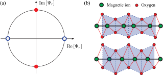
Figure 1: (Color online) (a) The two scenarios of nematic bond order parameter $\Psi_{r}=\langle S_{r}^{+}S_{r+1}^{+}\rangle=\langle{\cal O}^{a}\rangle+i\langle{\cal O}^{b}\rangle$: open and full circles represent the real, $\langle{\cal O}^{a}\rangle$, and imaginary, $\langle{\cal O}^{b}\rangle$ parts of the nematic order parameter, respectively. (b) Lattice distortions induced via spin-orbit coupling by the real (upper panel) and the imaginary (lower panel) parts of the bond nematic order parameter. Translational symmetry is broken in both cases, but the lattice distortion takes place along different directions. The bigger circles represent the magnetic transition-metal ions. The smaller circles represent the oxygen atoms that mediate the super-exchange interaction.

In this work we investigate the relevant effect of spin-orbit interaction on the 1D frustrated $J_{1}-J_{2}$ model. Based on our previous considerations, there are two possible scenarios: i) The field-induced transition from a quantum paramagnet to the nematic phase is replaced by a crossover (no discrete symmetry breaking); ii) The field-induced transition from a quantum paramagnet to the nematic phase is replaced by a discrete symmetry breaking. We can anticipate that the problem under consideration belongs to the second case because it is known that the magnon-pairs condense at a finite wave vector $\pm Q$. In other words, the nematic ordering breaks the translational symmetry, which is not affected by the inclusion of the spin-orbit interaction. In addition, the system has an additional $Z_{2}$ symmetry besides the $\pi$-rotation about the $z$-axis. This symmetry is the product of two operations, ${\cal T}{\cal R}(\pi)$, where ${\cal T}$ is the time reversal operator and ${\cal R}(\pi)$ is a $\pi$-rotation operator about an axis perpendicular to the field direction. As we explain below, the real part of the nematic order parameter, ${\cal O}^{a}$, preserves this $Z_{2}$ symmetry, while the imaginary part, ${\cal O}^{b}$, does not. Fig. 1 (a) shows the the different broken symmetry states associate with the stabilization of the real or imaginary part of the nematic order parameter.

In the following sections, we derive a phenomenological Ginzburg-Landau theory that is complemented by microscopic analytical and numerical calculations. Moreover, we demonstrate that the combination of a divergent nematic susceptibility and spin anisotropy stabilizes the real component of the nematic order parameter, ${\cal O}^{a}$, which in turn produces bond dimerization in most of the phase diagram. This bond ordering is accompanied by an orthorhombic distortion of the surrounding oxygen octahedron, as it is schematically shown in the upper panel of Fig. 1 (b). In contrast, the imaginary component of the “nematic” order parameter, ${\cal O}^{b}$, does not produce bond dimerization. If stabilized by other mechanisms, this phase would produce a local orthorhombic distortion of the surrounding oxygen octahedron along diagonal directions, as illustrated in the lower panel of Fig. 1 (b).

Given that bond dimerization couples to the lattice via magneto-elastic interaction and lowers the space group of the material under consideration, the combined effect of high spin nematic susceptibility and spin anisotropy can in principle be detected with X-rays. In addition, the incommensurate bond-density wave expected for smaller values of $J_{2}/|J_{1}|$ should lead to a double-horn shape of the nuclear magnetic resonance (NMR) line. These conclusions can shed light on the search for the spin “nematic ordering” predicted on the basis of a U(1) invariant $J_{1}-J_{2}$ Heisenberg model.

The structure of this paper is as follows. In Sec. II, we introduce a simple model Hamiltonian in which the U(1) symmetry is reduced to Z₂ via the inclusion of an Ising term (symmetric anisotropy). In Sec. III we consider a simple Ginzburg-Landau (GL) theory, which describes the possible scenarios. The phenomenological input parameters of the GL theory are calculated in Sec. IV by means of an analytical approach to the microscopic Hamiltonian. The results of this analytical approach are confirmed by numerical Density Matrix Renormalization Group (DMRG) calculations presented in Sec. V. The general implications of our results for experimental studies of unconventional magnetic ordering in quasi-1D frustrated compounds are discussed in Sec. VI.

II Model Hamiltonian

We consider a spin-$1/2$ anisotropic Heisenberg model on a 1D chain with ferromagnetic nearest-neighbor exchange, $J_{1}<0$, and antiferromagnetic next nearest neighbor exchange $J_{2}>0$:

$$\mathcal{H} =J_{1}\sum_{j}{\bf S}_{j}\cdot{\bf S}_{j+1}+J_{2}\sum_{j}{\bf S}_{j}\cdot{\bf S}_{j+2}-h\sum_{j}S_{j}^{z}$$

$$\;\;+\alpha\sum_{j}S_{j}^{x}S_{j+1}^{x},$$ (1)

The last term is an Ising interaction that in real materials arises from the combined effect of spin-orbit coupling and lattice anisotropy. This term reduces the U(1) symmetry of continuous spin rotations about the field axis to $Z_{2}$. We note that the U(1) symmetry is restored if the magnetic field is applied along the $x$-direction. However, in real quasi-1D materials, the U(1) symmetry is not present for any direction of the magnetic field because of the interaction with other chains ref:nematic1 . In spite of these considerations, the U(1) invariant model has been invoked to describe various quasi-1D transition metal compounds. sato13

Based on the U(1) invariant model ($\alpha=0$), several authors proposed that nematic quasi-long range ordering should be observed right below the saturation field $h_{\rm sat}$ ref:nematic1 ; ref:nematic2 ; ref:nematic3 ; ref:nematic4 ; ref:nematic5 ; ref:nematic5b ; ref:nematic5c ; ref:nematic5d . $h_{\rm sat}$ is finite only for $J_{2}>|J_{1}|/4$ because the zero field ground state is ferromagnetic for $J_{2}\leq|J_{1}|/4$. The nematic ordering corresponds to a Bose-Einstein condensation of two-magnon bound states with a local order parameter $\langle S_{j}^{+}S_{j+1}^{+}\rangle$. The attractive magnon-magnon interaction is provided by the ferromagnetic nearest-neighbor exchange $J_{1}$. The ratio $J_{2}/\lvert J_{1}\rvert$ controls the total momentum $\pm Q$ of the two-magnon bound state. $Q$ is incommensurate for small values of $J_{2}/\lvert J_{1}\rvert$ and it is equal to $\pi$ for $J_{2}/\lvert J_{1}\rvert\geq 0.375$.

In general, the continuous SU(2) symmetry of the Heisenberg interaction is broken down to a discrete symmetry group in real materials ref:1DmaterialA2 ; ref:1Dmaterial2 . Even for an idealized single-chain system, the exchange interaction turns out to be anisotropic, instead of SU(2) invariant, once the spin-orbit interaction is included. This is so because an isolated chain has only one symmetry axis parallel to the chain direction ($x$-direction in our notation). In other words, the exchange interaction between spin components parallel to the chain direction is different from the exchange interaction between the spin components perpendicular to the chain direction, as it is clear from the $\alpha$-term in Eq. (1). Consequently, the pure 1D Hamiltonian has only discrete point group symmetries if the external magnetic field is not parallel to the chain direction. For the case under consideration (magnetic field perpendicular to the chain direction), the U(1) symmetry of the Heisenberg model is reduced to a discrete $Z_{2}$ symmetry corresponding to a $\pi$-rotation about the $z$-axis ${\cal R}_{z}(\pi):\;S_{r}^{z}\rightarrow S_{r}^{z},S_{r}^{x,y}\rightarrow-S_{r}^{x,y}$. Correspondingly, the spin components $S_{r}^{\pm}$ transform into $e^{\pm i\phi}S_{r}^{\pm}$ under a rotation by $\phi$ about the $z$-axis. This means that the nematic order parameter, $\langle S_{r}^{+}S_{r}^{+}\rangle$, transforms into $e^{i2\phi}\langle S_{r}^{+}S_{r}^{+}\rangle$, implying that it is invariant under $\pi$-rotations, as expected for a director. The inclusion of spin anisotropy then forces us to reconsider the problem because other symmetries (different from rotations) have to be invoked to characterize the phase that replaces the nematic quasi-long range ordering.

Besides the above mentioned $\pi$ rotation about the $z$-axis, the Hamiltonian of Eq. (1) is invariant under the product of the time reversal operation and a $\pi$-rotation about the $y$-axis, ${\cal T}{\cal R}_{y}(\pi)$, which changes the sign of the $y$ spin component: $S_{r}^{x,z}\rightarrow S_{r}^{x,z},S_{r}^{y}\rightarrow-S_{r}^{y}$. The real-part of the nematic order parameter,

$$\Re\langle S_{r}^{+}S_{r+1}^{+}\rangle=\langle S_{r}^{x}S_{r+1}^{x}-S_{r}^{y}S_{r+1}^{y}\rangle\equiv\langle{\cal O}^{a}(r)\rangle,$$ (2)

remains invariant under this transformation. In contrast, the imaginary part,

$$\Im\langle S_{r}^{+}S_{r+1}^{+}\rangle=\langle S_{r}^{x}S_{r+1}^{y}+S_{r}^{y}S_{r+1}^{x}\rangle,$$ (3)

changes sign. Finally, the nematic order parameter breaks the translational symmetry because the magnon-pairs condense at a finite momentum $\pm Q$. This symmetry is then expected to break spontaneously for $\alpha\neq 0$, as long as $Q$ is commensurate.

Based on this simple symmetry analysis, the spin anisotropy should stabilize a state that breaks the translational symmetry (in a strong or a weak sense) and select either the real or the imaginary part of the original nematic order parameter. Only one of these two components should be selected, as supposed to some linear combination, because they belong to different irreducible representations of the point group of $\mathcal{H}$.

III Ginzburg-Landau theory

The attractive interaction between magnons arising from the ferromagnetic nearest-neighbor interaction, leads to two-magnon bound states for $J_{2}/|J_{1}|>1/4$. The minimum energy of the two-magnon bound state is achieved for a finite value, $\pm Q$, of the center of mass momentum. The two-magnon bound states condense for $h<h_{c}$ (note that $h_{c}$ is higher than the field required to close the single-magnon gap). The two-magnon condensate is characterized by a two component complex order parameter $\Psi_{\pm Q}$ (macroscopic wave function of condensate) whenever $Q\neq-Q$. The spin-orbit interaction generates an effective coupling between these two components, as it can be inferred from the lowest order expansion of the Ginzburg-Landau free energy:

$${\cal F}=r\left(|\Psi_{Q}|^{2}+|\Psi_{\bar{Q}}|^{2}\right)+u\left(\Psi_{Q}^{*}\Psi_{\bar{Q}}^{*}+\Psi_{\bar{Q}}\Psi_{Q}\right),$$ (4)

where $\bar{Q}=-Q$. Due to the $Z_{2}$ symmetry restriction, the complex field $\Psi_{\pm Q}$ is fixed up to a phase factor $\pm 1$. We have also assumed that $u$ is real based on the underlying microscopic theory. We will first assume $Q=\pi$ which is the condensation wave vector for $J_{2}>J_{2c}$ ($J_{2c}\simeq 0.375\rvert J_{1}\rvert$ for $\alpha=0$). Given that $Q=\pi$ is invariant under spatial inversion, we have $\Psi_{\pi}=\Psi_{-\pi}$. Then, upon minimization of the free energy, we obtain a real order parameter $\Psi_{\pi}$ for $u<0$, and a purely imaginary order parameter for $u>0$. In the original spin language, we have $\Psi_{\pi}=\frac{1}{N}\sum_{r}e^{i\pi r}\langle S_{r}^{-}S_{r+1}^{-}\rangle$, whose real and imaginary parts are

$${\cal O}^{a} =\sum(-1)^{r}\langle S_{r}^{x}S_{r+1}^{x}-S_{r}^{y}S_{r+1}^{y}\rangle,$$ (5)

$${\cal O}^{b} =-\sum(-1)^{r}\langle S_{r}^{x}S_{r+1}^{y}+S_{r}^{y}S_{r+1}^{x}\rangle.$$ (6)

A real order parameter only breaks the translational symmetry, while an imaginary order parameter breaks additional symmetries, such as, ${\cal T}{\cal R}_{y}(\pi):\;S_{r}^{x,z}\rightarrow S_{r}^{x,z},S_{r}^{y}\rightarrow-S_{r}^{y}$. In both cases, the system should develop long-range ordering at $T=0$ because only discrete symmetries are broken. We note that the spin anisotropy corresponds to a uniform nematic field that couples linearly to the uniform component of the nematic order parameter $\Psi_{0}=\frac{1}{N}\sum_{r}\langle S_{r}^{-}S_{r+1}^{-}\rangle$, implying that $\Psi_{0}$ becomes finite for a finite $\alpha$. As we will see next, the interference between $\Psi_{0}$ and the $\pi$ component, $\Psi_{\pi}$, of the real part of the order parameter leads to a real space modulation (dimerization) of the expectation value of nearest-neighbor bond operators.

In general, the nematic order parameter is a complex number, $|\Psi_{\pi}|e^{i\theta}$, where $\theta=0$ and $\theta=\frac{\pi}{2}$ correspond to ${\cal O}^{a}$ and ${\cal O}^{b}$, respectively. The real space version of these order parameters is obtained via a Fourier transformation,

$${\cal O}^{a}(r) =\Psi_{0}+2(-1)^{r}\Psi_{\pi}\cos(\theta),$$ (7)

$${\cal O}^{b}(r) =2(-1)^{r}\Psi_{\pi}\sin(\theta),$$ (8)

which gives the real and imaginary parts of $\Psi_{r}=\langle S_{r}^{-}S_{r+1}^{-}\rangle$. It is clear that the amplitude of the real component, ${\cal O}^{a}(r)$, is modulated in real space for finite values of the spin-orbit interaction ($\Psi_{0}\neq 0$). In contrast, only the phase is modulated for $\alpha=0$. In other words, the spin-orbit coupling induces a dimerized bond ordering if the real component of the original nematic order parameter is selected. This interference between the $0$ and $\pi$ components of ${\cal O}^{a}$ also leads to a magnon pair density wave:

$$n_{pair}(r) =\langle\Psi_{r}^{\dagger}\Psi_{r}\rangle\simeq\langle\Psi_{r}\rangle^{*}\langle\Psi_{r}\rangle$$

$$=\Psi_{0}^{2}+4\Psi_{\pi}^{2}+4(-1)^{r}\Psi_{0}\Psi_{\pi}\cos(\theta).$$ (9)

It follows that the long range ${\cal O}^{a}$ ordering is accompanied by another bond ordering associated with the longitudinal spin component

$$\langle S_{r}^{z}S_{r+1}^{z}\rangle\simeq\langle\Psi_{r}\rangle^{*}\langle\Psi_{r}\rangle+const..$$ (10)

This is just the usual bond dimerization that appears in spin-Peierls systems. Miller82 Indeed, Eq. (10) implies that the usual bond order parameter, $\langle{\bf S}_{r}\cdot{\bf S}_{r+1}\rangle$, must also exhibit dimerization.

The condensation wave vector becomes incommensurate ($Q<\pi$) for smaller values of $J_{2}/|J_{1}|$ (about $0.375$ for $\alpha=0$). In this case we need to consider a two component order parameter with phases $e^{i\theta_{\pm}}$ for $\pm Q$. Minimization of the free energy leads to $\theta_{+}+\theta_{-}=0\text{ mod }(2\pi)$ for $u<0$ and to $\phi_{+}+\phi_{-}=\pi\text{ mod }(2\pi)$ for $u>0$. The complex order parameter does not have a fixed phase because of the additional $U(1)$ phase factor $e^{\pm iQr}$, arising from translational symmetry. This $U(1)$ symmetry precludes long-range order for the single-chain problem. The free energy minimization also leads to the same amplitude for both components of the order parameter: $|\Psi_{Q}|=|\Psi_{\bar{Q}}|$, implying that the ground state must exhibit quasi-long range bond density wave order ${\cal O}^{a}(r)=\Psi_{0}+2|\Psi_{Q}|\cos(Qr)$ or ${\cal O}^{b}(r)=2|\Psi_{Q}|\sin(Qr)$.

IV Microscopic theory

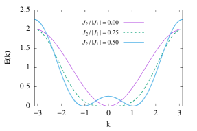
Figure 2: (Color online) Single-magnon dispersion produced from the non-interacting part of the Hamiltonian [see Eq (IV)] with $\alpha=0$. The dashed line corresponds to the Lifshitz point where the single-magnon dispersion becomes quartic at low-enrgies because the single minimum splits into two minima.

Our discussion in the previous section indicates that two different kinds of bond order can be induced by spin anisotropy. To determine which order parameter is selected we need to consider the underlying microscopic theory. To this end, we use the Jordan-Wigner transformation to reformulate the spin Hamiltonian (1) as a model for interacting spinless fermions:

$$S_{j}^{+} =e^{-i\pi\sum_{k=1}^{j-1}n_{k}}c_{j}^{\dagger},$$ (11)

$$S_{j}^{-} =e^{i\pi\sum_{k=1}^{j-1}n_{k}}c_{j},$$ (12)

$$S_{j}^{z} =c_{j}^{\dagger}c_{j}-\frac{1}{2},$$ (13)

where $c_{j}$ is the fermionic spinless operator which represents a spin flip on site $j$. The fermionic Hamiltonian is defined as

$${\cal H}={\cal H}_{0}+{\cal H}_{int},$$

where

$${\cal H}_{0} =\sum_{k}c_{k}^{\dagger}c_{k}\left(J_{1}\cos k+J_{2}\cos 2k-\left(h+J_{1}+J_{2}\right)\right)$$

$$+i\frac{\alpha}{4}\sum_{k}\sin k\left(c_{k}^{\dagger}c_{-k}^{\dagger}-c_{-k}c_{k}\right).$$ (14)

For $\alpha=0$, the single-particle spectrum, corresponding to single-magnon excitations, has a minimum at $k_{0}=\arccos(-\frac{J_{1}}{4J_{2}})$ if $4J_{2}>|J_{1}|$ and at $k_{0}=0$ if $4J_{2}<|J_{1}|$. Fig. 2 shows the evolution of the single-particle spectrum with increasing $J_{2}/\rvert J_{1}\rvert$. The spin-orbit interaction ($\alpha\neq 0$) breaks the $U(1)$ symmetry and the fermion number is no longer conserved. The interacting part of the Hamiltonian is

$${\cal H}_{int} =\frac{1}{2N}\sum_{Q,q,p}U(Q,q,p)c_{\frac{Q}{2}+p}^{\dagger}c_{\frac{Q}{2}-p}^{\dagger}c_{\frac{Q}{2}-q}c_{\frac{Q}{2}+q},$$ (15)

where

$$U(Q,q,p) =2({J_{1}}+2J_{2}\cos Q)\sin(q)\sin(p)$$ (16)

$$+2{J_{2}}\sin(2q)\sin(2p).$$ (17)

The effective attractive interaction between nearest neighbor sites, $J_{1}+2J_{2}\cos Q$, is maximized at $Q=\pi$. Therefore, the lowest energy “two-magnon” bound state is expected to have this momentum for large enough $J_{2}/|J_{1}|$.

In the isotropic limit, the nematic phase corresponds to a magnon pair condensate. This state can be approximated by a coherent state built with the two-particle wave function of the bound state. In presence of magnetic anisotropy, the particle number is not conserved because particles can be created or annihilated in pairs. The Hamiltonian eigenstates can then be grouped into two categories based on the particle number parity. The following analysis assumes that the magnetic anisotropy is weak ($\alpha\ll 1$), implying that the finite particle density induced by the spin anisotropy term above and at the critical field, $h_{c}$ can be made arbitrarily small for small enough values of $\alpha$. This condition also guarantees that two magnon condensation is still the dominant instability for $\alpha\neq 0$. For this reason, we will still refer to the bound state as a “two-magnon” bound states (adiabatic continuation) and we will use the two-particle Green’s function to compute the energy of the two-magnon modes. The two-particle Green’s function is obtained from the two-particle scattering amplitude by solving the corresponding Bethe-Salpeter equation.

IV.1 Bogoliubov representation

The above non-interacting fermionic Hamiltonian can be diagonalized with a Bogoliubov transformation,

$$c_{k} =\left(u_{k}\alpha_{k}+v_{k}\alpha_{-k}^{\dagger}\right)e^{i\frac{\pi}{4}},$$ (18)

$$c_{k}^{\dagger} =\left(u_{k}\alpha_{k}^{\dagger}+v_{k}\alpha_{-k}\right)e^{-i\frac{\pi}{4}},$$ (19)

where

$$u_{k} =\sqrt{\frac{1}{2}\left(1+\frac{\epsilon_{k}}{E_{k}}\right)},$$ (20)

$$v_{k} =-sign(\Delta_{k})\sqrt{\frac{1}{2}\left(1-\frac{\epsilon_{k}}{E_{k}}\right)},$$ (21)

with $E_{k}=\sqrt{\epsilon_{k}^{2}+4\Delta_{k}^{2}}$, $\Delta_{k}=\frac{\alpha}{4}\sin k$ and

$$\epsilon_{k}=J_{1}\cos k+J_{2}\cos 2k-\left(h+J_{1}+J_{2}\right).$$ (22)

The diagonal Hamiltonian

$${\cal H}_{0}=\sum_{k}E_{k}\alpha_{k}^{\dagger}\alpha_{k}+E_{0}.$$ (23)

leads to the non-interacting Green’s function

$$iG_{0}(k,\omega) =\langle 0|{\cal T}\alpha_{k}^{\dagger}\alpha_{k}|0\rangle=\frac{i}{\omega-E_{k}+i0^{+}}.$$ (24)

The next step is to write the interaction vertex in terms of the Bogoliubov quasi-particle operators. The normal interaction term is

$${\cal H}_{int}^{N} =\frac{1}{4N}\sum_{Q,q,p}\Gamma_{Q}^{(0)N}(q,p)\alpha_{\frac{Q}{2}+p}^{\dagger}\alpha_{\frac{Q}{2}-p}^{\dagger}\alpha_{\frac{Q}{2}-q}\alpha_{\frac{Q}{2}+q},$$ (25)

with a normal interaction vertex

$$\Gamma_{Q}^{(0)N}(q,p) =2U(Q,q,p)\times\left(u_{\frac{Q}{2}+p}u_{\frac{Q}{2}-p}u_{\frac{Q}{2}-q}u_{\frac{Q}{2}+q}+v_{\frac{Q}{2}+p}v_{\frac{Q}{2}-p}v_{\frac{Q}{2}-q}v_{\frac{Q}{2}+q}\right)$$ (26)

$$-4U(p+q,\frac{Q-p+q}{2},\frac{Q+p-q}{2})\left(u_{\frac{Q}{2}+p}v_{\frac{Q}{2}-p}v_{\frac{Q}{2}-q}u_{\frac{Q}{2}+q}+u_{\frac{Q}{2}-p}v_{\frac{Q}{2}+p}v_{\frac{Q}{2}+q}u_{\frac{Q}{2}-q}\right).$$ (27)

We can verify that $\Gamma_{Q}^{(0)N}(q,p)=\Gamma_{Q}^{(0)N}(-q,-p)$ due to the fermionic statistics. Furthermore, $\Gamma_{Q}^{(0)N}(q,p)=\Gamma_{\bar{Q}}^{(0)N}(-q,-p)=\Gamma_{\bar{Q}}^{(0)N}(q,p)$ because of inversion symmetry. The interaction vertex has been symmetrized with respect to the exchange of external lines. The anomalous interaction terms of the form $\alpha^{\dagger}\alpha^{\dagger}\alpha^{\dagger}\alpha^{\dagger}$ and $\alpha\alpha\alpha\alpha$ are

$${\cal H}_{int}^{A} =\frac{1}{4!N}\sum_{Q,q,p}\Gamma_{Q}^{(0)A}(q,p)\left(\alpha_{\frac{Q}{2}+p}^{\dagger}\alpha_{\frac{Q}{2}-p}^{\dagger}\alpha_{-\frac{Q}{2}+q}^{\dagger}\alpha_{-\frac{Q}{2}-q}^{\dagger}+h.c.\right),$$ (28)

with an anomalous interaction vertex

$$\Gamma_{Q}^{(0)A}(q,p) =2U(Q,q,p)\left(u_{\frac{Q}{2}+p}u_{\frac{Q}{2}-p}v_{\frac{Q}{2}-q}v_{\frac{Q}{2}+q}+v_{\frac{Q}{2}+p}v_{\frac{Q}{2}-p}u_{\frac{Q}{2}-q}u_{\frac{Q}{2}+q}\right)$$ (29)

$$-2U(p+q,\frac{Q-p+q}{2},\frac{Q+p-q}{2})\left(u_{\frac{Q}{2}+p}v_{\frac{Q}{2}-p}u_{\frac{Q}{2}-q}v_{\frac{Q}{2}+q}+v_{\frac{Q}{2}+p}u_{\frac{Q}{2}-p}v_{\frac{Q}{2}-q}u_{\frac{Q}{2}+q}\right)$$ (30)

$$+2U(p-q,\frac{Q+p+q}{2},\frac{Q-p-q}{2})\left(v_{\frac{Q}{2}+p}u_{\frac{Q}{2}-p}u_{\frac{Q}{2}-q}v_{\frac{Q}{2}+q}+u_{\frac{Q}{2}+p}v_{\frac{Q}{2}-p}v_{\frac{Q}{2}-q}u_{\frac{Q}{2}+q}\right).$$ (31)

We can verify that $\Gamma_{Q}^{(0)A}(q,p)=\Gamma_{\bar{Q}}^{(0)A}(p,q)=\Gamma_{Q}^{(0)A}(-q,-p)$ due to fermionic statistics and $\Gamma_{Q}^{(0)A}(q,p)=\Gamma_{\bar{Q}}^{(0)A}(-q,-p)=\Gamma_{\bar{Q}}^{(0)A}(q,p)$ due to inversion symmetry. This interaction vertex has also been symmetrized with respect to the exchange of external lines.

The remaining anomalous terms ($\alpha^{\dagger}\alpha^{\dagger}\alpha^{\dagger}\alpha$ and $\alpha\alpha\alpha\alpha^{\dagger}$) will not be considered because they give subdominant contributions (in an expansion in powers of $\alpha$) to the effective anomalous interaction vertex shown in Fig. 3. We note that the nature of the order parameter is determined by the effective anomalous interaction vertex because the effective normal vertex preserves the U(1) symmetry of ${\cal H}(\alpha=0)$.

Finally, we also note the existence of additional diagrams which are obtained by exchange of the external legs of the diagrams shown in Fig. 3. These diagrams are of the same order in an expansion in powers of $\alpha$. However, for the purpose of calculating the two magnon bound state, they can be neglected because they give contributions that remain regular in the proximity of the critical field $h=h_{c}$.

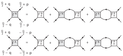
Figure 3: Ladder diagrams for the normal and anomalous scattering amplitudes $\Gamma^{N}$ and $\Gamma^{A}$.

IV.2 Bethe-Salpeter equation

In the dilute limit, the scattering amplitude can be calculated by summing up the ladder diagrams shown in Fig. 3. This sum leads to the Bethe-Salpeter equation BSE :

$$\Gamma_{\omega Q}^{N}(q,p) =\Gamma_{Q}^{(0)N}(q,p)-\frac{1}{2N}\sum_{k}\frac{\Gamma_{Q}^{(0)N}(Q;q,k)\Gamma_{\omega Q}^{N}(k,p)}{E_{\frac{Q}{2}+k}+E_{\frac{Q}{2}-k}-\omega-i0^{+}}-\frac{1}{2N}\sum_{k}\frac{\Gamma_{Q}^{(0)A}(q,k)\Gamma_{\omega Q}^{A}(k,p)}{E_{\frac{Q}{2}+k}+E_{\frac{Q}{2}-k}+\omega-i0^{+}},$$ (32)

$$\Gamma_{\omega Q}^{A}(q,p) =\Gamma_{Q}^{(0)A}(q,p)-\frac{1}{2N}\sum_{k}\frac{\Gamma_{Q}^{(0)N}(q,k)\Gamma_{\omega Q}^{A}(k,p)}{E_{\frac{Q}{2}+k}+E_{\frac{Q}{2}-k}+\omega-i0^{+}}-\frac{1}{2N}\sum_{k}\frac{\Gamma_{Q}^{(0)A}(q,k)\Gamma_{\omega Q}^{N}(k,p)}{E_{\frac{Q}{2}+k}+E_{\frac{Q}{2}-k}-\omega-i0^{+}},$$ (33)

where $\Gamma_{Q}^{(0)N/A}$ is the bare scattering amplitude of the normal and anomalous type. The energy of the magnon pair bound state can be extracted from the poles of the scattering amplitude. For a wide range of $J_{2}/|J_{1}|$ values, the bound state dispersion has its minimum at $Q=\pi$. The energy of the two-magnon bound state increases with $\alpha$, implying that the critical field for the “two-magnon” condensation decreases relative to the saturation field of the isotropic ($\alpha=0$) Hamiltonian.

For the isotropic Heisenberg model, the condensate wave function has a $U(1)$ phase freedom. The spin anisotropy reduces this freedom to $Z_{2}$. The Ginzburg-Landau theory tells us that the phase of the macroscopic wave function can either be real or imaginary depending on the sign of the effective anomalous coupling parameter $u$. In this section we determine the phase of the wave function and also include a microscopic calculation of the parameter $u$. These properties are enclosed in the scattering amplitude obtained from the solution of the Bethe-Salpeter equation. Our analysis shows that wave function of the magnon pair condensate is real, implying that the dominant order parameter is ${\cal O}^{a}$.

IV.2.1 Wave function of the bound state

We start by introducing the two-magnon Green’s function, which can be easily obtained through the scattering amplitude $\Gamma_{\omega Q}^{N/A}(q,p)$:

$$G^{(2)}(\omega,Q;q,p) =G_{0}^{(2)}(\omega,Q;,q,p)+\frac{1}{4}G_{0}^{(2)}(\omega,Q;q,q^{\prime})$$

$$\times\Gamma_{\omega Q}^{N}(q^{\prime},p^{\prime})G_{0}^{(2)}(\omega,Q;p^{\prime},p),$$ (34)

$$G_{A}^{(2)}(\omega,Q;q,p) =\frac{1}{4}G_{0}^{(2)}(-\omega,-Q;-q,-q^{\prime})$$

$$\times\Gamma_{\omega Q}^{A}(q^{\prime},p^{\prime})G_{0}^{(2)}(-\omega,-Q;-p^{\prime},-p),$$ (35)

where $G_{0}^{(2)}$ is the non-interacting two particle Green’s function:

$$G_{0}^{(2)}(\omega,Q;q,q^{\prime})=\frac{\delta(q-q^{\prime})-\delta(q+q^{\prime})}{\omega-E_{\frac{Q}{2}+q}-E_{\frac{Q}{2}-q}+i0^{+}}.$$ (36)

The Lehmann representation shows explicitly that the two particle Green’s function has the following singular behavior near the pole of bound state, $\omega\sim\omega_{B}$:

$$G_{N}^{(2)}(\omega,Q;q,p) \sim\frac{\psi_{Q}(p)\psi_{Q}^{*}(q)}{\omega-\omega_{B}+i0^{+}}+\text{regular terms},$$ (37)

$$G_{A}^{(2)}(\omega,Q;q,p) \sim\frac{\psi_{Q}(p)\phi_{-Q}(q)}{\omega-\omega_{B}+i0^{+}}+\text{regular terms},$$ (38)

where the regular terms come from higher excited states and $\omega_{B}>0$ is the bound state energy relative to the ground state. The projection of the bound state wave function on the two-magnon sector is obtained from the residue of the pole,

$$\psi_{Q}(p) =\langle G|\alpha_{\frac{Q}{2}+p}\alpha_{\frac{Q}{2}-p}|B\rangle_{Q},$$ (39)

$$\phi_{\bar{Q}}^{*}(p) =\langle G|\alpha_{-\frac{Q}{2}-p}^{\dagger}\alpha_{-\frac{Q}{2}+p}^{\dagger}|B\rangle_{Q},$$ (40)

where $|B\rangle$ is the ket of the bound state and $|G\rangle$ the ground state. Due to the anomalous interaction arising from the spin anisotropy term, the bound state wave function is a linear combination of states with different particle number. The poles of the two particle Green’s function given by Eqs. (34) and (35) are obtained after inserting the scattering amplitude, $\Gamma_{\omega Q}^{N/A}(q,p)$, which results from the Bethe-Salpeter equation. According to Eqs. (39) and (40), the bound state wave function is then obtained by extracting the residue near the pole $\omega_{B}$. For $Q=\pi$, the bound state wave functions, $\psi_{\pi}(p)$ and $\phi_{\pi}(p)$, are even under spatial inversion. This result is found to be correct for all $J_{2}/|J_{1}|$ ratios and for any value of the bound state energy $\omega_{B}$, indicating that the broken symmetry state below the critical field must preserve the spatial inversion symmetry.

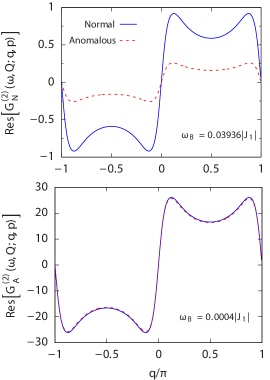
Figure 4: Residue of the two particle normal/anomalous Green’s function near the pole $\omega_{B}$ in frequency space for: (a) $\omega_{B}/|J_{1}|=0.03936$ and (b) $\omega_{B}/|J_{1}|=0.0004$ (close to the “two-magnon” condensation point). The other parameters are taken as $J_{2}/|J_{1}|=1,\alpha=0.2$, momentum $p=0.9\pi$. We find the normal (blue solid line) and anomalous (red dotted line) two-particle Green’s function become the same upon approaching the critical condensation point.

As the system approaches the critical field corresponding to the onset of the “two-magnon” condensate, $\omega_{B}\rightarrow 0$, the normal and the anomalous Green’s function become exactly the same (see Fig. 4). Consequently, the particle pair wave function, $\psi_{Q}(p)$, is exactly the same as the hole pair wave function $\phi_{\bar{Q}}^{*}(p)$. This is a manifestation of an emergent particle-hole symmetry at zero energy, which sets a constraint on the phase of the bound state wave function. If we describe the condensate state as a coherent state built with the two-body bound state wave function, the phases $\theta_{\pm}$ for the macroscopic components $\Psi_{\pm Q}$ are given by $\psi_{Q}(p)$ and $\phi_{\bar{Q}}(p)$, respectively. The relationship $\psi_{Q}(p)=\phi_{\bar{Q}}^{*}(p)$ indicates that $\theta_{+}+\theta_{-}=0$, which leads to a real order parameter $\langle S_{r}^{+}S_{r+1}^{+}\rangle$ in real space.

Beyond the condensation point, the new ground state, $|G\rangle$, is characterized by the order parameter $\Phi_{Q}(q)=\langle G|\alpha_{\frac{Q}{2}+q}\alpha_{\frac{Q}{2}-q}|G\rangle$. The coherent representation enables us to identify the bound state wave functions $\psi_{Q}(p)$ and $\phi_{\bar{Q}}(p)$ with the two component order parameter, $\Phi_{Q}(p)$ and $\Phi_{\bar{Q}}(p)$, that was discussed in Section III. This correspondence leads to the self-consistent equation for the order parameter based on the Bethe-Salpeter equation, from which one can straightforwardly confirm which order is favored. The analysis becomes more transparent by adopting an equivalent but more straightforward approach. We just introduce a small pairing field term into the Hamiltonian, which couples to the order parameter:

$${\cal H}_{paring} =h_{Q}^{*}\sum_{q}\alpha_{\frac{Q}{2}+q}\alpha_{\frac{Q}{2}-q}+h_{\bar{Q}}^{*}\sum_{q}\alpha_{\frac{\bar{Q}}{2}+q}\alpha_{\frac{\bar{Q}}{2}-q}+h.c..$$ (41)

The renormalized pairing fields $h_{Q}^{R},h_{\bar{Q}}^{R}$ are indicated by the ladder series of vertex corrections in Fig. 5. The pairing susceptibility diverges at the condensation point, implying that the order parameter develops spontaneously beyond this point, i.e., in absence of the pairing fields $h_{Q}$ and $h_{\bar{Q}}$. The order parameter in momentum space, $\Phi_{Q}(q)=\langle\alpha_{\frac{Q}{2}+q}\alpha_{\frac{Q}{2}-q}\rangle$, can be calculated as $\Phi_{Q}(q)=-h_{Q}^{R}(q)/\Omega_{q}$. Therefore, the ladder series of vertex corrections in Fig. 5 leads to the following self-consistent equation:

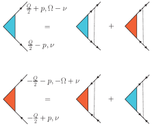
Figure 5: Ladder diagrams for the pairing field $h_{\pm Q}^{R}(q)$. The blue (red) vertex represents the renormalized pairing field at $Q$ ($-Q$). The dashed lines represent the symmetrized interaction vertexes in Eqs. (26) and (29).

$$\sum_{k}\left(\Omega_{Q}(q)\delta_{q,k}+\frac{1}{2N}\Gamma_{Q}^{(0)N}(q,k)\pm\Gamma_{Q}^{(0)A}(k,q)\right)\Phi_{Q}^{\pm}(k)=0,$$ (42)

where $\Omega_{Q}(q)=E_{{Q\over 2}+q}+E_{{Q\over 2}-q}$ is the energy of a two-magnon excitation and

$$\Phi_{Q}^{\pm}(k)=\Phi_{Q}(k)\pm\Phi_{-Q}^{*}(k).$$ (43)

The order parameters $\Phi_{Q}^{\pm}(k)$ become finite when the corresponding matrix in Eq. (42) is singular. For $Q=\pi$, $\Phi_{\pi}^{+}(k)$ coincides with imaginary part of $\Phi_{\pi}(k)$, while $\Phi_{\pi}^{-}(k)$ is the real part. The numerical calculation shows that the order parameter $\Phi_{\pi}(k)$ is purely imaginary for $Q=\pi$ and that it satisfies $\Phi_{Q}(k)=\Phi_{-Q}^{*}(k)$ for $Q<\pi$.

To understand the meaning of this result in real space, we just need to consider the order parameter $\langle S_{r+1}^{-}S_{r}^{-}\rangle$, which is given by $\langle c_{r+1}c_{r}\rangle$ in terms of the Jordan-Wigner fermionic annihilation operators. By applying Fourier and Bogoliubov transformations, we find

$$\langle S_{r+1}^{-}S_{r}^{-}\rangle=\Psi_{0}-\frac{1}{N}\sum_{q}u_{\frac{Q}{2}+q}u_{\frac{Q}{2}-q}\sin q$$

$$\times[\Phi_{Q}(q)e^{i\frac{Q}{2}}e^{iQr}+\Phi_{\bar{Q}}(q)e^{i\frac{\bar{Q}}{2}}e^{i\bar{Q}r}]-\frac{1}{N}\sum_{q}v_{\frac{Q}{2}+q}v_{\frac{Q}{2}-q}$$

$$\times\sin q[\Phi_{\bar{Q}}^{*}(q)e^{i\frac{Q}{2}}e^{iQr}+\Phi_{Q}^{*}(q)e^{i\frac{\bar{Q}}{2}}e^{i\bar{Q}r}].$$ (44)

The relationship $\Phi_{Q}(q)=\Phi_{\bar{Q}}^{*}(q)$ implies that the real space order parameter is

$$\langle S_{r+1}^{-}S_{r}^{-}\rangle =\Psi_{0}-\frac{2}{N}\sum_{q}\left(u_{\frac{Q}{2}+q}u_{\frac{Q}{2}-q}+v_{\frac{Q}{2}+q}v_{\frac{Q}{2}-q}\right)$$

$$|\Phi_{Q}(q)|\sin q\cos\left(Qr+Q/2+\phi_{+}\right),$$ (45)

where $\phi_{+}$ is the phase of $\Phi_{Q}(q)$. Therefore, the order parameter $\langle S_{r+1}^{-}S_{r}^{-}\rangle$ is real.

IV.2.2 Microscopic calculation of phenomenological parameters

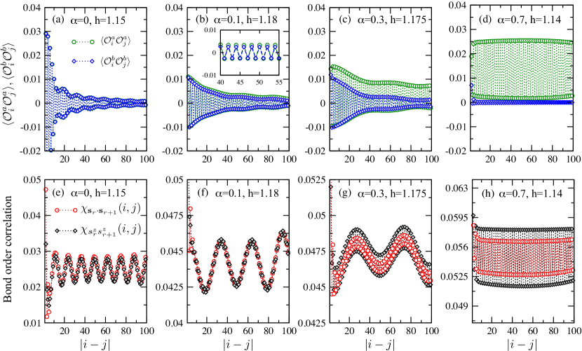
Figure 6: (Color online) DMRG simulation for a spin chain of length $L=160$ with open boundary condition. The measurement is made in the bulk with $i=30$ and $31<j\leq 130$. (a)-(d) show the correlation function of two types of bond order for different values of $\alpha$. (e)-(h) show the correlation function of the bond orders $\chi_{{\bf S}_{r}\cdot{\bf S}_{r+1}}(i,j)=\langle{\bf S}_{i}\cdot{\bf S}_{i+1}{\bf S}_{j}\cdot{\bf S}_{j+1}\rangle$ and $\chi_{S^{z}_{r}S^{z}_{r+1}}(i,j)=\langle{S}^{z}_{i}{S}^{z}_{i+1}{S}^{z}_{j}{S}^{z}_{j+1}\rangle$. The frustration ratio is $J_{2}/|J_{1}|=0.9659$ and the magnetic field is close to the critical field for each value of $\alpha$.

To provide a microscopic derivation of the phenomenological parameters $r$ and $u$ we express the Ginzburg-Landau free energy in its diagonal form:

$${\cal F}=\frac{r+u}{2}|\Psi_{+}|^{2}+\frac{r-u}{2}|\Psi_{-}|^{2},$$ (46)

where $\Psi_{\pm}=\Psi_{Q}\pm\Psi_{\bar{Q}}^{*}$ and $\Psi_{Q}$ is the Fourier transform of the bond order parameter $\langle S_{r}^{-}S_{r+1}^{-}\rangle$. The order parameter can be expressed in terms of the fermionic Bogoliubov quasi-particles,

$$\Psi_{\pm}=-\frac{e^{iQ/2}}{\sqrt{N}}\sum_{q}\sin(q)(u_{\frac{Q}{2}+q}u_{\frac{Q}{2}-q}\pm v_{\frac{Q}{2}+q}v_{\frac{Q}{2}-q})\Phi_{\pm}(q),$$ (47)

where $\Phi_{\pm}(q)=\Phi_{Q}(q)\pm\Phi_{\bar{Q}}^{*}(q)$ and $\Phi_{Q}(q)=\langle\alpha_{\frac{Q}{2}+q}\alpha_{\frac{Q}{2}-q}\rangle$. From Eq. (46), we can identify the phenomenological parameters with the inverse of the corresponding static susceptibilities:

$$r\pm u=\langle\Psi^{\dagger}_{\pm}\Psi_{\pm}\rangle^{-1}=\left(\chi_{\pm}\right)^{-1}.$$ (48)

In other words, $\chi_{\pm}$ are the response functions to pairing fields that couple linearly to the $\Psi_{\pm}$ order parameters given in Eq. (47):

$$\chi_{\pm} =-\frac{2}{N}\sum_{qp}\frac{\sin q\sin pB_{q}^{\pm}B_{p}^{\pm}}{\Omega_{Q}(q)\Omega_{Q}(p)}\left(\Gamma_{0Q}^{N}(q,p)\pm\Gamma_{0Q}^{A}(q,p)\right)$$

$$+\frac{2}{N}\sum_{q}\frac{\sin^{2}q(B_{q}^{\pm})^{2}}{\Omega_{Q}(q)},$$ (49)

where $\Gamma_{0Q}^{N/A}(q,p)$ is the scattering amplitude at zero frequency, $\Omega_{Q}(q)=E_{\frac{Q}{2}+q}+E_{\frac{Q}{2}-q}$ and $B_{q}^{\pm}=u_{\frac{Q}{2}+q}u_{\frac{Q}{2}-q}\pm v_{\frac{Q}{2}+q}v_{\frac{Q}{2}-q}$. The second term is the non-interacting susceptibility of the Bogoliubov fermions, which is negligible near the critical point where both $\Gamma_{0Q}^{N}(q,p)$ and $\Gamma_{0Q}^{A}(q,p)$ diverge. The finite $u$ value arises from the non-zero anomalous scattering amplitude, $\Gamma_{0Q}^{A}(q,p)$, which forces the two susceptibilities $\chi_{Q}^{\pm}$ to be different:

$$u=\frac{\left(\chi_{Q}^{+}\right)^{-1}-\left(\chi_{Q}^{-}\right)^{-1}}{2}.$$ (50)

Numerically, we always find $u<0$ for different ratios of $J_{2}/J_{1}$, in agreement with our previous discussions.

V Numerical simulations

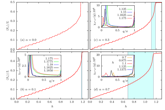
Figure 7: (Color online) Magnetization curve obtained from DMRG simulations for the same parameters as in Fig. 6. The shaded (light blue) region indicates the extension of the dimerized phase. The inset shows the Fourier transform of the real space correlation function $\chi_{S^{z}_{r}S^{z}_{r+1}}(i,j)$ for different magnetic field value. The peak at $q=\pi$ is a clear indicator of bond dimerization arising from the combination of two-magnon condensation and spin anisotropy ($\alpha\neq 0$).

The above theoretical analysis for small $\alpha$ indicates that the spin anisotropy stabilizes a dimerized ground state. In this section we present DMRG calculations ref:dmrg1 ; ref:dmrg2 for the anisotropic 1D spin Hamiltonian ${\cal H}$, which confirm this analysis. The calculations have been done right below the critical field for chains of $L=160$ spins with open boundary conditions. We used up to 400 states and kept the truncation tolerance below $10^{-8}$ throughout the DMRG iterations. We did 6 full sweeps of finite algorithm of DMRG to get well converged observables. Fig. 6 shows the correlation functions for the real and imaginary parts of the nematic order parameter, ${\cal O}^{a}$, ${\cal O}^{b}$, for the “pair-density" operator $S_{i}^{z}S_{i+1}^{z}$, and for the bond operators ${\bf S}_{i}\cdot{\bf S}_{i+1}$, for different values of $\alpha$. The frustration ratio is taken as $J_{2}/J_{1}=0.9659$, which gives rise to a lowest energy “two-magnon” bound state with center of mass momentum equal to $\pi$. In agreement with the “two-magnon” calculation, the correlation functions of the order parameters ${\cal O}^{a}$ and ${\cal O}^{b}$ oscillate with wave vector $\pi$. The long wave length oscillations are just a consequence of the open boundary conditions and the large spin density wave susceptibility. Note, however, that the incommensurate nature of oscillations precludes the possibility of having long range spin density wave ordering (the incommensurate spin density wave ordering breaks the continuous U(1) symmetry group of translations).

The first column in Fig. 6 with $\alpha=0$ corresponds to the U(1) symmetric case for which all the correlators exhibit the expected power law behavior. The order parameters ${\cal O}^{a}$ and ${\cal O}^{b}$ are connected by a $\pi/4$ spin rotation about the $z$-axis, which is a symmetry of the Hamiltonian for $\alpha=0$. Correspondingly, both correlation functions exhibit an identical power-law decay. The bond and the pair density correlators also exhibit a power law decay with long wave length oscillations, which are magnified by the open boundary conditions ref:chiral2 .

The upper panels of Fig. 6 show that the real component of the nematic order parameter dominates over the imaginary part and develops long range ordering for nonzero $\alpha$. The amplitude of the order parameter increases with $\alpha$. As expected from the previous analysis, the pair density, $S_{i}^{z}S_{i+1}^{z}$, and the bond, ${\bf S}_{i}\cdot{\bf S}_{i+1}$, operators become dimerized as a consequence of the coexistence of uniform and staggered components of the ${\cal O}^{a}$ order parameter. We recall that the uniform component is directly induced by the $\alpha$ term of the Hamiltonian, while the staggered ($\pi$) component is spontaneously generated. The dimerization is identified by Fourier transforming the real space correlation functions shown in Figs. 6(e-h). This information is provided in the insets of Fig. 7, which show a clear peak at $Q=\pi$. It is also clear from Figs. 6(e-h) that the dimerization order parameter becomes more robust upon increasing $\alpha$. Moreover, the insets of Fig. 7 show that the Friedel oscillations of $\langle S_{i}^{z}\rangle$ are strongly suppressed for $\alpha=0.7$, i.e., for a large amplitude of the dimerization order parameter. Consistently with these results, Fig. 7 shows that the dimerized phase (shaded region) becomes stable over a larger window of magnetic field values as we increase $\alpha$. The same figure includes the field dependence of the magnetization curve for different values of $\alpha$. As expected, the slope of the magnetization curve above the critical field increases with $\alpha$ and the magnetization saturates asymptotically for $H\rightarrow\infty$.

VI Discussion and summary

Finally, we discuss the consequences of our theoretical study on the experimental search for nematic phases in various quasi-1D materials. We first note that two previous works studied the role of an XXZ magnetic anisotropy, which preserves the $U(1)$ symmetry of the spin Hamiltonian. Both works concluded that the effect of the U(1) invariant spin anisotropy is to stabilize the nematic phase. Similarly, we are finding that the effect of a U(1) symmetry breaking anisotropy is to stabilize the dimerized phase, which is a “direct descendant" of the nematic ordering (real part of the nematic order parameter).

The spin anisotropy of the quasi-1D compound LiCuVO₄ is approximately $\alpha=0.1$. ref:Z2material1 ; ref:1Dmaterial2 ; ref:1Dmaterial3 ; ref:1Dmaterial6 ; LiCuVO4 ; LiCuVO4b ; observation The results of our simulations for this value of $\alpha$ [see Figs. 6 (b) and (f)] clearly show that the bond-bond correlation function develops a visible $\pi$ ordering (dimerization). This is a salient experimental signature that can be detected with X-rays. Rb₂Cu₂Mo₃O₁₂ is another quasi-1D $J_{1}$-$J_{2}$ frustrated magnet ref:1DmaterialA1 ; ref:1DmaterialA2 with $J_{2}/\lvert J_{1}\rvert\simeq 0.33$. This value falls in the “mutipolar" phase (quasi-condensate of $n$-magnon bound states with $n>2$) of the U(1) invariant spin model. Indeed, the nematic phase becomes unstable for $J_{2}/\rvert J_{1}\rvert<0.37$. Although we have not considered the situation of multipolar orderings of higher order than nematic, our simple GL analysis shows that the $\alpha$-term should once again select the real or the imaginary part of the multipolar order parameter.

A more recent experimental work reports evidence of a gapped “nematic ordering" for the quasi-1D $J_{1}-J_{2}$ compound LiCuSbO₄. grafe2016 Nuclear magnetic resonance (NMR) measurements indicate the opening of a rather large spin gap above a critical magnetic field value $H_{c1}\simeq 13$T. Conventional explanations for the origin of this spin gap, such as saturation of the magnetization or the presence of a staggered Dzyaloshinskii-Moriya (DM) interaction have been ruled out by the experiments. Moreover, the absence of a kink in the low temperature magnetization vs. field curve is consistent with an XYZ magnetic anisotropy. Based on our analysis, this U(1) symmetry breaking anisotropy is responsible for the the spin gap that is inferred from the NMR measurements. According to Ref. grafe2016 the value of the spin anisotropy is $\alpha\simeq 0.08$. In addition, a $J_{2}/\rvert J_{1}\rvert\simeq 0.28$ ratio is obtained from a fit of the magnetization curve with a pure one-dimensional Hamiltonian. This ratio puts the material outside the region of stability of the nematic phase ref:chiral2 (higher multipolar orderings are expected for $J_{2}/\rvert J_{1}\lesssim 0.367$). However, Ref. LiCusbO4 reports a significantly larger ratio $J_{2}/\rvert J_{1}\rvert\simeq 0.45$, which falls in the nematic phase of the U(1) invariant Hamiltonian. ref:chiral2 . If this $J_{2}/\rvert J_{1}\rvert$ ratio is correct, the gapped high-field spin phase of this compound must correspond to a spin dimerized phase. However, further inspection of this material grafe2016 shows that the lattice is already dimerized (consecutive bonds are not equivalent) implying a continuous crossover between the dimerized spin phase and the high field paramagnetic state.

In summary, we have demonstrated that the spin-orbit interaction has important consequences for the field-induced spin nematic ordering of U(1) invariant frustrated models. The symmetry reduction of ${\cal H}$ due to the presence of the Ising term renders the nematic order parameter inapplicable. However, the real and imaginary parts of the nematic bond order parameter still break discrete symmetries, which can be directly related with observable quantities. Our analytical and numerical results demonstrate that the spin-orbit interaction stabilizes a bond density wave (bond dimerization for $Q=\pi$) which couples to the lattice via the magneto-elastic effect. These results are confirmed by our DMRG simulations. Given that the spin-orbit interaction is ubiquitous in nature and that continuous symmetries are never strictly present in real magnets, our study indicates that the proposed nematic ordering is likely to be replaced by bond dimerization in systems described by a $J_{1}$-$J_{2}$ model with $|J_{2}|/|J_{1}|\gtrsim 0.38$. Even in quasi-1D systems, which are approximately described by a U(1) invariant $XXZ$ model, the application of a magnetic field perpendicular to the chains should induce the dimerized state that we are proposing here.

- (1) Vivien Zapf, Marcelo Jaime, and C. D. Batista, Rev. Mod. Phys. 86, 563 (2014).
- (2) L. Balents, Nature 464, 199 (2010).
- (3) A. V. Chubukov and O. A. Starykh, Phys. Rev. Lett. 110, 217210 (2013).
- (4) Toshiya Hikihara, Lars Kecke, Tsutomu Momoi, and Akira Furusaki, Phys. Rev. B 78, 144404 (2008).
- (5) Gia-Wei Chern, C. J. Fennie, and O. Tchernyshyov, Phys. Rev. B 74, 060405 (R) (2006).
- (6) P. W. Anderson, Mater. Res. Bull., 8, 153 (1973).
- (7) Fradkin E., Field Theories of Condensed Matter Systems (Addison-Wesley, Reading) 1991.
- (8) F. L. Pratt, P. J. Baker, S. J. Blundell, T. Lancaster, S. Ohira-Kawamura, C. Baines, Y. Shimizu, K. Kanoda, I. Watanabe, and G. Saito, Nature. 471, 612 (2011).
- (9) X. G. Wen, F. Wilczek, and A. Zee, Phys. Rev. B 39, 11413 (1989).
- (10) M. E. Zhitomirsky and H. Tsunetsugu, Europhys. Lett., 92, 37001 (2010).
- (11) L. Kecke, T. Momoi, and A. Furusaki, Phys. Rev. B 76, 060407 (2007).
- (12) T. Hikihara, L. Kecke, T. Momoi, and A Furusaki, Phys. Rev. B 78, 144404 (2008).
- (13) A. V. Chubukov, Phys. Rev. B 44, 4693 (1991).
- (14) J. Sudan, A. Lüscher, and A. M. Läuchli, Phys. Rev. B 80, 140402(R) (2009).
- (15) A. Lüscher, J. Sudan, and A. Lüscher, J. Phys. Conf. Ser. 145, 012057 (2009).
- (16) T. Vekua, A. Honecker, H.-J. Mikeska, and F. Heidrich-Meisner, Phys. Rev. B 76, 174420 (2007).
- (17) A. V. Syromyatnikov, Phys. Rev. B 86, 014423 (2012).
- (18) A. Läuchli, J. C. Domenge, C. Lhuillier, P. Sindzingre, and M. Troyer, Phys. Rev. Lett. 95, 137206 (2005).
- (19) Nic Shannon, Tsutomu Momoi, and Philippe Sindzingre, Phys. Rev. Lett. 96, 027213 (2006).
- (20) G. Marmorini and T. Momoi, Phys. Rev. B 89, 134425 (2014).
- (21) Ryuichi Shindou and Tsutomu Momoi, Phys. Rev. B 80, 064410 (2009).
- (22) H. T. Ueda and T. Momoi, Phys. Rev. B 87, 144417 (2013).
- (23) Emika Takata, Tsutomu Momoi, and Masaki Oshikawa, arXiv: 1510.02373.
- (24) M. Hase, H. Kuroe, K. Ozawa, O. Suzuki, H. Kitazawa, G. Kido, and T. Sekine, Phys. Rev. B 70, 104426 2004 .
- (25) Y. Yasui, R. Okazaki, I. Terasaki, M. Hase, M. Hagihala, T. Masuda, and T. Sakakibara, JPS Conf. Proc. 3, 014014 (2014)
- (26) M. Enderle, C. Mukherjee, B. Fák, R. K. Kremer, J.-M. Broto, H. Rosner, S.-L. Drechsler, J. Richter, J. Malek, A. Prokofiev, W. Assmus, S. Pujol, J.-L. Raggazzoni, H. Rakoto, M. Rheinstädter and H. M. Rønnow, Europhys. Lett., 70 (2), 237 (2005).
- (27) J. S. Miller (Ed.): Extended Linear Chain Compounds. Plenum Press, New York and London 1982.
- (28) H. A. KrugvonNidda, L. E. Svistov, M. V. Eremin, R. M. Eremina, A. Loidl, V. Kataev, A. Validov, A. Prokofiev, and W. Amus, Phys. Rev. B 65, 134445 (2002).
- (29) N. Büttgen, W. Kraetschmer, L. E. Svistov, L. A. Prozorova, and A. Prokofiev, Phys. Rev. B 81, 052403 (2010).
- (30) N. Büttgen, H.-A. Krug von Nidda, L. E. Svistov, L. A. Prozorova, A. Prokofiev, and W. Amus, Phys. Rev. B 76, 014440 (2007).
- (31) K. Nawa, M. Takigawa, M. Yoshida, and K. Yoshimura, Journal of the Physical Society of Japan 82, 094709 (2013).
- (32) N. Büttgen, K. Nawa, T. Fujita, M. Hagiwara, P. Kuhns, A. Prokovief, A. P. Reyes, L. E. Svistov, K. Yoshimura, and M. Takigawa, Phys. Rev. B 90, 134401 (2014).
- (33) F. Schrettle, S. Krohns, P. Lunkenheimer, J. Hemberger, N. Büttgen, H.-A. Krug von Nidda, A. V. Prokofiev, and A. Loidl, Phys. Rev. B 77, 144101 (2008).
- (34) M. G. Banks, F. Heidrich-Meisner, A. Honecker, H. Rakoto, J.-M. Broto and R. K. Kremer, J. Phys.: Condens. Matter 19 145227 (2007).
- (35) B.J. Gibson, R.K. Kremer, A.V. Prokofiev, W. Assmus, G.J. McIntyre, Physica B 350 e253 (2004).
- (36) K. Nawa, Y. Okamoto, A. Matsuo, K. Kindo, Y. Kitahara, S. Yoshida, S. Ikeda, S. Hara, T. Sakurai, S. Okubo, H. Ohta, H. Ohta, and Z. Hiroi, J. Phys. Soc. Jpn. 83, 103702 (2014).
- (37) K. Nawa, T. Yajima, Y. Okamoto, and Z. Hiroi, Inorg. Chem. 54, 5566 (2015).
- (38) H. -J. Grafe, S. Nishimoto, M. Iakovleva, E. Vavilova, L. Spillecke, A. Alfonsov, M.-I. Sturza, S. Wurmehl, H. Nojiri, H. Rosner, J. Richter, U.K. Röler, S.-L. Drechsler, V. Kataev, and B. Büchner, arxiv:1607.05164.
- (39) S. E. Dutton, M. Kumar, M. Mourigal, Z. Soos, J.-J. Wen, C. Broholm, N. Andersen, Q. Huang, M. Zbiri, R. Toft-Petersen, and R. J. Cava, Phys. Rev. Lett. 108, 187206 (2012).
- (40) B. Willenberg, M. Schäpers, A.U.B. Wolter, S. L. Drechsler, M. Reehuis, J.-U. Hoffmann, B. Buchner, A. J. Studer, K. C. Rule, B. Ouladdiaf, S. Sullow, and S. Nishimoto, Phys. Rev. Lett. 116, 047202 (2016).
- (41) H. T. Ueda and K. Totsuka, Phys. Rev. B 80, 014417 (2009).
- (42) M. Sato, T. Momoi, and A. Furusaki, Phys. Rev. B 79, 060406(R).
- (43) M. Sato, T. Hikihara, and T. Momoi, Phys. Rev. B 83, 064405 (2011).
- (44) A. Smerald and N. Shannon, Phys. Rev. B 93, 184419 (2016).
- (45) G. Jackeli and G. Khaliullin, Phys. Rev. Lett. 102, 017205 (2009).
- (46) M. Sato, T. Hikihara and T. Momoi, Phys. Rev. Lett. 110, 077206 (2013).
- (47) O. A. Starykh and L. Balents, Phys. Rev. B 89, 104407 (2014).
- (48) L. E. Svistov, T. Fujita, H. Yamaguchi, S. Kimura, K. Omura, A. Prokofiev, A. I. Smirnov, Z. Honda and M. Hagiwara, Jetp Lett. 93 21 (2011).
- (49) S. R. White, Phys. Rev. Lett. 69, 2863 (1992).
- (50) S. R. White, Phys. Rev. B 48, 10345 (1993).
- (51) H. Onishi, Journal of Physics: Conference Series 592, 012109 (2015).
- (52) S. Nishimoto, S. -L. Drechsler, R. Kuzian, J. Richter and J. vandenBrink, Phys. Rev. B 92, 214415 (2015).
- (53) M. Mourigal, M. Enderle, B. Fak, R. K. Kremer, J. M. Law, A. Schneidewind, A. Hiess and A. Prokofiev, Phys. Rev. Lett. 109, 027203 (2012)