Tuning Over-Relaxed ADMM

Abstract

The framework of Integral Quadratic Constraints (IQC) reduces the computation of upper bounds on the convergence rate of several optimization algorithms to a semi-definite program (SDP). In the case of over-relaxed Alternating Direction Method of Multipliers (ADMM), an explicit and closed form solution to this SDP was derived in our recent work [1]. The purpose of this paper is twofold. First, we summarize these results. Second, we explore one of its consequences which allows us to obtain general and simple formulas for optimal parameter selection. These results are valid for arbitrary strongly convex objective functions.

1 Introduction

Consider the optimization problem

$$\min_{x\in\mathbb{R}^{p},z\in\mathbb{R}^{q}}\{f(x)+g(z)\}\quad\text{subject to}\quad Ax+Bz=c,$$ (1)

where $A\in\mathbb{R}^{r\times p}$, $B\in\mathbb{R}^{r\times q}$, and $c\in\mathbb{R}^{r}$. We consider ADMM applied to problem (1) under the assumption that $f(x)$ is strongly convex and $g(z)$ is convex. ADMM is parametrized by $\alpha>0$ and $\rho>0$, and takes the form of Algorithm 1. Strictly speaking, this defines a family of algorithms, one per parameter choice.

In this paper, we tune ADMM by providing explicit and simple formulas for the parameters $\alpha$ and $\rho$, yielding the best possible asymptotic convergence rate among all first order methods. This is an immediate consequence of the results proposed in [1].

A classical choice of parameters is $\alpha=1$ and $\rho=1$, which can be substantially suboptimal. Several works have computed bounds on ADMM’s convergence rate for specific and restricted ranges of $\alpha$ and $\rho$. However, the IQC formalism introduced in [2], allowed [3] to reduce the analysis of this entire family of solvers to finding solutions to an SDP. This SDP has multiple solutions, each one giving a different bound on the convergence rate of ADMM, some better than others. This SDP was analyzed numerically, and a single explicit feasible solution was given when $\kappa$ is sufficiently large ($\kappa$ is related to the ratio of the smallest to the largest “curvature” of $f$). It was also shown via a lower bound, that for large $\kappa$, it is not possible to extract from this SDP a rate much better than this.

A closed form solution to this SDP was recently obtained in [1], which express the convergence rate explicitly in terms of the parameters of ADMM and condition numbers of problem (1). Moreover, it was shown that the closed form solution is the best possible one can extract from the SDP. Here we revisit these results, and from this explicit solution we provide formulas for the optimal parameters $\alpha$ and $\rho$ of ADMM in terms of condition numbers and curvature of $f$.

Algorithm 1 Family of over-relaxed ADMM schemes (parameters $\alpha$, $\rho$)

1:  Input: $f$, $g$, $A$, $B$, $c$;

2:  Initialize $z_{0},u_{0}$

3:  repeat

4:     $x_{t+1}=\operatorname*{arg\,min}_{x}f(x)+\tfrac{\rho}{2}\|Ax+Bz_{t}-c+u_{t}\|^{2}$

5:     $z_{t+1}=\operatorname*{arg\,min}_{z}g(z)+\tfrac{\rho}{2}\|\alpha Ax_{t+1}-(1-\alpha)Bz_{t}+Bz-\alpha c+u_{t}\|^{2}$

6:     $u_{t+1}=u_{t}+\alpha Ax_{t+1}-(1-\alpha)Bz_{t}+Bz_{t+1}-\alpha c$

7:  until stopping criteria

2 Main Results

Assumption 1.

Throughout the paper, we assume that $f$ and $g$ in (1) are convex, closed and proper, $A$ is invertible, and $B$ has full column rank. Given a function $h:\mathbb{R}^{p}\mapsto\mathbb{R}$ we say that $h\in S_{p}(m,L)$ if and only if $0<m\leq L<\infty$ and $m\|x-y\|^{2}\leq\left(\nabla h(x)-\nabla h(y)\right)^{T}(x-y)\leq L\|x-y\|^{2}$. In other words, $S_{p}(m,L)$ is the set of strongly convex functions with Lipschitz continuous gradients. We assume that $f\in S_{p}(m,L)$ and $g\in S_{q}(0,\infty)$.

We start by recalling the main result of [3]. It was shown that the iterative scheme of Algorithm 1 can be written as a dynamical system with a feedback signal related to the gradient of $f$ and sub-gradient of $g$. The stability of this dynamical system is then related to the convergence rate of Algorithm 1, which in turn involves numerically solving a $4\times 4$ SDP, as stated below in Theorem 2. We state this in a simplified form, and refer the reader to [3] for more details. Let us first introduce the constants

$$\rho_{0}=\rho\,(\hat{m}\hat{L})^{-1/2},\qquad\kappa=\kappa_{f}\kappa_{A}^{2}$$ (2)

where $\hat{m}={m}/{\sigma_{1}^{2}(A)}$, $\hat{L}={L}/{\sigma_{p}^{2}(A)}$, and $\kappa_{f}=L/m$. Here $\sigma_{1}(A)$ and $\sigma_{p}(A)$ denote the largest and smallest singular value of matrix $A$, respectively. In addition, $\kappa_{A}=\sigma_{1}(A)/\sigma_{p}(A)$ is the condition number of $A$.

Theorem 2 (See [3]).

Let the sequences $\left\{x_{t}\right\}$, $\left\{z_{t}\right\}$, and $\left\{u_{t}\right\}$ evolve according to Algorithm 1. Let $\varphi_{t}=\left[z_{t},u_{t}\right]^{T}$ and $\varphi_{*}$ be a fixed point. Let $0<\tau<1$ be such that

$$E-\tau^{2}F+G\preceq 0,$$ (3)

where $E$, $F$ and $G$ are $4\times 4$ matrices depending on $\alpha$, $\rho_{0}$, and $\kappa$. Moreover, $G$ is symmetric, $E$ is positive semi-definite, and $F=\left(\begin{smallmatrix}P&0\\ 0&0\end{smallmatrix}\right)$ where $P$ is a $2\times 2$ positive-definite matrix (the exact definitions are not important for this paper). For all $t\geq 0$ we thus have

$$\|\varphi_{t}-\varphi_{*}\|\leq\kappa_{B}\sqrt{\kappa_{P}}\,\tau^{t}\|\varphi_{0}-\varphi_{*}\|.$$ (4)

As already pointed out in [3], the weakness of Theorem 2 is that $\tau$ is not explicitly given as a function of $\kappa$, $\rho_{0}$, and $\alpha$. The factor $\kappa_{P}$ in (4) is also not explicitly given. Therefore, for given values of $\kappa$, $\rho_{0}$, and $\alpha$, one must perform a numerical search to find the minimal $\tau$ such that (3) is feasible, and thus obtain the best possible bound on the convergence rate of ADMM. Notice, however, that it is unclear a priori whether other methods could improve on this bound. This numerical approach was carried out in [3] using a binary search on $\tau$, justified by the fact that the positive semi-definite property of $F$ implies that the eigenvalues of $E-\tau^{2}G+G$ decrease monotonically with $\tau$. Notice that one might have to scan the parameter space $(\alpha,\rho_{0})$ multiple times for a problem with a specific value of $\kappa$. Even from a practical point of view, this procedure may introduce delays. For instance, if (3) is used in an adaptive scheme where after every few iterations we estimate a local value of $\kappa$ and then re-optimize $\alpha$ and $\rho$.

Therefore, it is not only theoretically desirable to have an explicit expression for the smallest $\tau$ that (3) can provide, but it may also be useful in practical applications. Such result was proposed in [1], and reproduced below in Theorem 3. Let us first introduce the function

$$\chi(x)=\max(x,x^{-1})\geq 1\quad\mbox{for $x\in\mathbb{R}>0$}.$$ (5)

Theorem 3 (See [1]).

Let $0<\alpha<2$, $\kappa\geq 1$, and $\rho_{0}>0$. The convergence rate of Algorithm 1 satisfies

$$\|\varphi_{t}-\varphi_{*}\|\leq\kappa_{B}\sqrt{\chi(\eta)}\,\tau_{A}^{\,t}\|\varphi_{0}-\varphi_{*}\|$$ (6)

where

$$\tau_{A}=1-\dfrac{\alpha}{1+\chi(\rho_{0})\sqrt{\kappa}}\quad\mbox{and}\quad\eta=\dfrac{\alpha}{2-\alpha}\cdot\dfrac{\chi(\rho_{0})\sqrt{\kappa}-1}{\chi(\rho_{0})\sqrt{\kappa}+1}.$$ (7)

Moreover, $\tau_{A}$ in (7) is the smallest possible $\tau$ which solves (3).

No other proof strategy can give a better general upper bound than (7) since $\tau_{A}$ is actually attainable. For instance, choosing $f(x)=\tfrac{1}{2}x^{T}Qx$, where $Q=\text{diag}(m,L)$, $g(z)=0$, $A=I$, $B=-I$, and $c=0$, the convergence rate of ADMM is given exactly by the formula of $\tau_{A}$ in (7) for any values of $\kappa>1$, $0<\alpha<2$ and $\rho_{0}>0$.

As a consequence of Theorem 3, we now present an explicit formula for optimal parameter selection of Algorithm 1.

Corollary 4 (Optimal Parameter Selection).

The best asymptotic convergence rate of over-relaxed ADMM, for $\alpha\in(0,2)$ and $\rho\in(0,\infty)$, is given by

$$\inf_{\alpha,\rho}\tau_{A}=1-\frac{2}{1+\sqrt{\kappa}},$$ (8)

where, we recall, $\kappa=\big{(}\tfrac{\sigma_{1}(A)}{\sigma_{p}(A)}\big{)}^{2}\tfrac{L}{m}$, and is achieved by letting $\alpha\to 2^{-}$ and $\rho=\tfrac{\sqrt{mL}}{\sigma_{1}(A)\sigma_{p}(A)}$. Furthermore, for a fixed iteration number $t$, the upper bound (6) is minimized by

$$\alpha=\begin{cases}1+\dfrac{1}{\chi(\rho_{0})\sqrt{\kappa}}&\quad\mbox{if $t\leq\chi(\rho_{0})\sqrt{\kappa}$,}\\ 1+\dfrac{1+\sqrt{1+4t^{2}-4t\chi(\rho_{0})\sqrt{\kappa}}}{2t}&\quad\mbox{if $t>\chi(\rho_{0})\sqrt{\kappa}$.}\end{cases}$$ (9)

Note that the optimal $\alpha$ and $\rho$ in Corollary 4 are expressed only in terms of condition numbers of problem (1), i.e. singular values of $A$ and bounds on the curvature of $f$. The matrix $B$ affects convergence but not the optimal choice of parameters. The function $g$ does not affect the bound on the convergence rate. The above tuning rule optimizes a general bound that holds simultaneously for all problems with the same $\kappa$. There is no tighter bound than this for the same general setting. However, this does not mean that for a specific problem a better bound with different tuning parameters cannot be found.

Related Work.

Two of the most explicit bounds that resemble (7) are found in [6, 7] and [8]. In [6, 7] the Douglas-Rachford splitting method is analyzed, which is different but related to the scheme considered in this paper. For a problem similar to (1), it gives a rate bound of $1-{\alpha}/{(1+\sqrt{\kappa_{f}})}$, where $\alpha$ is a step size and $\kappa_{f}=L/m$. ADMM to problem (1) with $\alpha=1$ and $\rho_{0}=1$ is considered in [8], and give an approximate rate bound of $1-{1}/{\sqrt{\kappa}}+O({\kappa^{-1}})$, where $\kappa=\kappa_{f}\kappa^{2}_{A}$. There are other works on ADMM with exact bound calculations. For example, [9] focus on distributed ADMM but only for the non-relaxed version. Explicit convergence rate and optimal parameters are given in [4], however, only for the particular case of quadratic objectives. Similar expressions for the convergence rate were proposed in in [10]. These expressions are upper bounds which are optimized, but it is not possible to prove they are the best possible. In addition, this work do not focus on over-relaxed ADMM. Finally, [11] and [12] also study over-relaxed ADMM. They provide upper bounds, but again, cannot prove these are the best possible. In [12] one can find a table that gives a good summary of known bounds under different assumptions, none of which overlaps with our work.

3 Numerical results

Let us compare numerical solutions to the SDP in Theorem 2 with the exact $\tau_{A}$ in equation (7). We use a binary search to find the best $\tau$ that solves (3). Figure 1 (a) shows the rate bound $\tau$ against $\kappa$ for several choices of parameters $(\alpha,\,\rho_{0})$. The dots correspond to the numerical solutions and the solid lines correspond to the exact formula $\tau_{A}$ in (7).

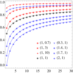
Figure 1: (a) Numeric (dots) and exact (lines) plot of $\tau$ versus $\kappa$ for different values of $\alpha$ and $\rho_{0}$. The best choice of parameters is $\rho_{0}=1$ and $\alpha=2$. (b) Numeric (dots) and exact (lines) plot of $\tau$ versus $\kappa$ with $\alpha>2$ and $\rho_{0}=1$. The dashed blue line corresponds to $\alpha=2$ in $\tau$. The shaded region contains curves $\tau$ for values of $\alpha$ not allowed in Theorem 3. Numerical solutions with $\alpha>2$ are restricted $1<\kappa\lesssim 11$. Notice that $\alpha>2$ does not produce better convergence rates than $1\leq\alpha<2$ through (7). (c) Numeric $\log\tau$ for different values of $\alpha$ when solving a classification problem.

Theorem 3 is valid only for $0<\alpha<2$ ($\tau_{A}$ can assume negative values for $\alpha>2$). However, Theorem 2 does not impose any restriction on $\alpha$, and holds even for $\alpha>2$ [3]. To explore the range $\alpha>2$, we numerically solve (3) as shown in Figure 1 (b). The dots correspond to the numerical solutions. The dashed blue line corresponds to (7) with $\alpha=2$, and it is the boundary of the shaded region in which (7) can have negative values and is no longer valid. Although Theorem 3 does not hold for $\alpha>2$, we deliberately included the solid lines representing (7) inside this region. Obviously, these curves do not match the numerical results.

The first important remark is that, for a given $\alpha>2$, we were unable to numerically find solutions for arbitrary $\kappa\geq 1$. For instance, for $\alpha=2.6$ we can only stay roughly on the interval $1<\kappa\lesssim 11$. The same behavior occurs for any $\alpha>2$, and the range of $\kappa$ becomes narrower as $\alpha$ increases. From the picture one can notice that $\tau=1$ is actually attained with finite $\kappa$, while for (7) this never happens; it rather approaches $\tau\to 1^{-}$ as $\kappa\to\infty$. Therefore, although it is feasible to solve (3) with $\alpha>2$, the solutions will be constrained to a small range of $\kappa$. The next question would be if Theorem 2 for $\alpha>2$ could possibly give a better rate bound than Theorem 3 with $1\leq\alpha<2$. We can see from the picture that this is probably not the case.

Now let us consider problem $\min_{\theta\in\mathbb{R}^{d}}\{f(\theta)+g(\theta)\}$ for the following regularized logistic regression to learn a sparse classifier from $N$ pairs $(x_{i},y_{i})$ where $x\in\mathbb{R}^{d}$ are features and $y\in\{-1,+1\}$ labels:

$$f(\theta)=\dfrac{1}{N}\sum_{i=1}^{N}\log\left(1+e^{-y_{i}\theta^{T}x_{i}}\right),\qquad g(\theta)=\mathbb{I}_{\infty}(\|\theta\|_{1}>\lambda),$$ (10)

where $\mathbb{I}_{\infty}(\bullet)=0$ if $(\bullet)$ is false and $\infty$ otherwise. In (1) we have $A=I$ and $B=-I$ so $\kappa_{A}=\kappa_{B}=1$. We generate $N/2$ points with $y_{i}=+1$ and $N/2$ points with $y_{i}=-1$ from a gaussian distribution $\mathcal{N}(0,\sigma I)$ in even $d$ dimensions. Then, for the $+1$ points, we shift half of the features by $+1/2$, and for the $-1$ points we shift the same half of the features by $-1/2$. Thus we have two classes of points whose centers are separated by $1$ along $d/2$ dimensions and the best hyper-plane separating these two classes has sparse coefficients. We use Algorithm 1 to solve this problem with several values of $\alpha$ and $\rho$, and plot $\log\left(\|\theta_{t}-\theta^{\star}\|\right)$ against iteration number $t$, where $\theta^{\star}$ is the optimum. If $N\geq d$, the function $f$ restricted to $\|\theta\|_{1}\leq\lambda$ is strongly convex with high probability. If $\lambda$ is small then $\|\theta\|$ is small and so $\nabla^{2}f(\theta)=\tfrac{1}{N}\sum^{N}_{i=1}\tfrac{x_{i}x^{T}_{i}}{\cosh(x^{T}_{i}\theta/2)}\approx\tfrac{1}{N}\sum^{N}_{i=1}x_{i}x^{T}_{i}$. From this, even without knowing $\theta$, we can estimate $\kappa_{f}$ which, for our choice of $N$, $d$, $\sigma$ and $\lambda$, is very large. Hence, our estimate for the best $\alpha$ using (9) is $1$. We see from Figure 1 (c) that this is not the best choice, which is $\alpha\approx 1.5$. Recall that our tuning rule is the best that holds uniformly across the family of strongly convex functions, but for specific problems it might be suboptimal.

4 Conclusion

We summarized the main results of [1], which is the content of Theorem 3. This introduces a new and explicit upper bound on the convergence rate of the family of over-relaxed ADMM, for arbitrary but strongly convex objective functions. This improves on previous work [3, 8]. In particular, the only explicit bound in [3] is a special case of (7) when $\kappa$ is large. Moreover, (7) is the best one can extract from the IQC framework of [2].

From this general bound we provide a tuning scheme for ADMM; Corollary 4. In [5] we find that $1-2/(1+\sqrt{\kappa})$, where $\kappa=m/L$, bounds the convergence rate of any first order method on $S_{p}(m,L)$. Thus the ADMM tuned as in (8) is close to optimal as a scheme for the entire family of strongly convex functions. However, as shown in the numerical experiments, for specific problems our tuning might be suboptimal.

References

- [1] G. França, J. Bento, “An Explicit Rate Bound for the Over-Relaxed ADMM”, ISIT (2016), arXiv:1512.02063v2 [stat.ML]
- [2] L. Lessard, B. Recht, A. Packard, “Analysis and design of optimization algorithms via integral quadratic constraints” (2014), arXiv:1408.3595 [math.OC]
- [3] R. Nishihara, L. Lessard, B. Recht, A. Packard, M. I. Jordan, “A General Analysis of the Convergence of ADMM”, Int. Conf. on Machine Learning 32 (2015), arXiv:1502.02009 [math.OC]
- [4] E. Ghadimi, A. Teixeira, I. Shames, “Optimal Parameter Selection for the Alternating Direction Method of Multipliers (ADMM): Quadratic Problems”, IEEE Trans. on Automatic Control 60 4 (2015)
- [5] Y. Nesterov, “Introductory Lectures on Convex Optimization: A Basic Course”, Kluwer Academic Publishers, Boston, MA, 2004
- [6] P. Giselsson, S. Boyd. “Diagonal scaling in Douglas-Rachford splitting and ADMM”, Decision and Control (CDC), (2014) IEEE 53rd Annual Conference
- [7] P. Giselsson, S. Boyd. “Linear Convergence and Metric Selection for Douglas-Rachford Splitting and ADMM”, IEEE Transactions on Automatic Control, (2016): 62
- [8] D. Wei, W. Yin. “On the global and linear convergence of the generalized alternating direction method of multipliers”, Journal of Scientific Computing (2012): 1-28
- [9] F. Iutzeler, P. Bianchi, P. Ciblat and W. Hachem. “Explicit convergence rate of a distributed alternating direction method of multipliers”, IEEE Transactions on Automatic Control (2016): 61
- [10] W. Shi, Q. Ling, K. Yuan, G. Wu and W. Yin. “On the linear convergence of the ADMM in decentralized consensus optimization”, IEEE Transactions on Signal Processing (2014): 62
- [11] D. Boley. “Local linear convergence of the alternating direction method of multipliers on quadratic or linear programs”, SIAM Journal on Optimization (2013): 23
- [12] D. Davis and W. Yin. “Faster convergence rates of relaxed Peaceman-Rachford and ADMM under regularity assumptions”, arXiv:1407.5210 [math.OC] (2014)