TreeClone: Reconstruction of Tumor Subclone Phylogeny Based on Mutation Pairs using Next Generation Sequencing Data
Abstract
We present TreeClone, a latent feature allocation model to reconstruct tumor subclones subject to phylogenetic evolution that mimics tumor evolution. Similar to most current methods, we consider data from next-generation sequencing of tumor DNA. Unlike most methods that use information in short reads mapped to single nucleotide variants (SNVs), we consider subclone phylogeny reconstruction using pairs of two proximal SNVs that can be mapped by the same short reads. As part of the Bayesian inference model, we construct a phylogenetic tree prior. The use of the tree structure in the prior greatly strengthens inference. Only subclones that can be explained by a phylogenetic tree are assigned non-negligible probabilities. The proposed Bayesian framework implies posterior distributions on the number of subclones, their genotypes, cellular proportions, and the phylogenetic tree spanned by the inferred subclones. The proposed method is validated against different sets of simulated and real-world data using single and multiple tumor samples. An open source software package is available at http://www.compgenome.org/treeclone.
Keywords: Latent feature model; Mutation pair; NGS data; Phylogenetic tree; Subclone; Tumor heterogeneity
1 Introduction
Initiated by somatic mutations in a single cell, cancer arises through Darwinian-like natural selection. The accumulation of subsequent genetic aberrations and the effects of selection over time result in the sequential clonal expansions of cells, finally leading to the development of a genetically aberrant tumor [Nowell (1976)]. This process, known as tumorigenesis, leads to genetically divergent subpopulations of tumor cells, also known as subclones [Bonavia et al. (2011); Marusyk et al. (2012)].
Deep next generation sequencing (NGS) of bulk tumor DNA samples makes it possible to examine the evolutionary history of individual tumors, based on the set of somatic mutations they have accumulated [Nik-Zainal et al. (2012)]. This is implemented by deconvoluting observed genomic data from a tumor into constituent signals corresponding to various subclones and by then reconstructing the relationship of these subclones in a phylogeny [Deshwar et al. (2015); Marass et al. (2017)]. Apart from phylogenetic relationship, tumor purity, subclones’ genotypes and cellular proportions are also coupled quantities to infer. Uncovering subclonal heterogeneity and their relationship is clinically important for better prognosis [Aparicio and Caldas (2013); Schwarz et al. (2015)]. Therefore there is a pressing need to develop robust methods for a reliable interpretation.
Numerous methods have been proposed for the subclonal reconstruction problem, including SciClone [Miller et al. (2014)], CloneHD [Fischer et al. (2014)], PyClone [Roth et al. (2014)], PyloWGS [Jiao et al. (2014); Deshwar et al. (2015)], Clomial [Zare et al. (2014)], BayClone [Sengupta et al. (2015)], Cloe [Marass et al. (2017)], and PairClone [Zhou et al. (2017)]. The reconstruction is typically based on short reads that are mapped to single nucleotide variants (SNVs) (few methods, for example, CloneHD, also consider somatic copy number aberrations, SCNA). Many methods based on SNV data utilize variant allele fractions (VAFs), that is, the fractions of alleles (or short reads) at each locus that carry mutations. Since humans are diploid, the expected VAFs of short reads for a homogeneous cell population should be 0, 0.5 or 1.0 for any locus in copy number neutral (copy number = 2) regions and after adjusting for tumor purity. Observing VAFs very different from 0, 0.5 or 1.0 is therefore evidence for heterogeneity. Most methods use only marginal SNVs. Recently, Zhou et al. (2017) have proposed to use pairs of proximal SNVs mapped by the same short reads, which carry more information than marginal SNVs, for more accurate subclone reconstruction. In terms of methodology, existing subclone reconstruction methods can be mainly divided into two categories: clustering-based and feature-allocation-based. The two categories are also referred to as indirect and direct reconstructions in Marass et al. (2017), depending on whether the subclonal genotypes are indirectly or directly inferred. Clustering-based methods, including SciClone, PyClone and PhyloWGS, first infer SNV clusters based on observed VAFs and then reconstruct subclonal genotypes based on the clusters. The phylogenetic relationship among the subclones can be inferred by imposing hierarchy among the SNV clusters. On the other hand, feature-allocation-based methods (e.g., Clomial, BayClone, Cloe or PairClone) treat subclones as latent features and directly infer subclonal genotypes. Most of the feature-allocation-based methods assume that the features (subclones) are conditionally independent and thus are not able to infer the phylogenetic relationship among the subclones. Recently, Marass et al. (2017) have developed a model allowing for dependency among the features to infer the tumor phylogenetic tree.
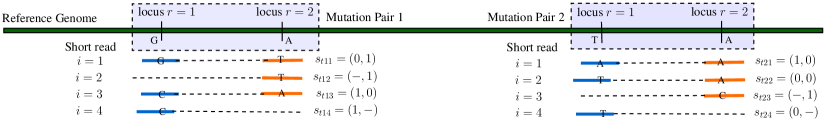
In the upcoming discussion we assume that the available data are from () samples from a single patient and the main inference goal is intra-tumor heterogeneity. We present a novel approach to reconstruct tumor subclones and their corresponding phylogenetic tree based on mutation pairs. Here a mutation pair refers to a pair of proximal SNVs on the genomes that can be simultaneously mapped by the same paired-end short reads, with one SNV on each end. In other words, mutation pairs can be phased by short reads. See Fig. 1 for an illustration. Short reads mapped to only one of the SNV loci are treated as partially missing paired-end reads and are not excluded from our approach. This idea of working with phased mutation pairs was introduced in Zhou et al. (2017). We build on this work and develop a novel and entirely different inference approach by explicitly modeling the underlying phylogenetic relationship. That is, we model tumor heterogeneity based on a representation of a phylogenetic tree of tumor cell subpopulations. A prior probability model on such phylogenetic trees induces a dependent prior on the mutation profiles of latent tumor cell subpopulations. Part of this construction is that the phylogenetic tree of tumor cell subpopulations is included as a random quantity in the Bayesian model. Like most existing methods, we only consider mutation pairs in copy number neutral region i.e. copy number two. The proposed inference aims to reconstruct (i) subclones defined by the haplotypes across all the mutation pairs, (ii) cellular proportion of each subclone, and (iii) a phylogenetic tree spanned by the subclones.
Next we introduce some notation to formally represent the described data and model structure. Consider an NGS data set with mutation pairs shared across all () samples. We assume that the samples are composed of homogeneous subclones. The number of subclones is unknown and becomes one of the model parameters. We use a matrix to represent the subclones, in which each column of represents a subclone and each row represents a mutation pair. That is, the element of the matrix corresponds to subclone and mutation pair . Each is itself again a matrix. It is a matrix that represents the genotypes of the two alleles of the mutation pair. See Fig. 2(b). An important step in the model construction is that the columns (subclones) of form a phylogenetic tree . The tree encodes the parent-child relationship across the subclones. A detailed construction of the tree and a prior probability model of and are introduced later. Lastly, we denote with the cellular proportions of the subclones in sample where for all and . Using NGS data we infer , , and based on a simple idea that variant reads can only arise from subclones with variant alleles consistent with an underlying phylogeny. We develop a tree-based latent feature allocation model (LFAM) to implement this reconstruction. Mutation pairs are the objects of the LFAM, and subclones are the latent features chosen by the mutation pairs.
The previous brief outline of data and model structure already highlights two key features of the proposed approach: the use of phylogenetic tree structure and data on mutation pairs. The latter has important advantages. Mutation pairs contain phasing information that improves the accuracy of subclone reconstruction. If two nucleotides reside on the same short read, we know that they must appear in the same DNA strand in a subclone. For example, consider a scenario with one mutation pair and two subclones. Suppose the reference genome allele is (A, G) for that mutation pair, with the notion that A and G are phased by the same DNA strand. Suppose the two subclones have diploid genomes at the two loci and the genotypes for both DNA strands are ((C, G), (A, T)) for subclone , and ((C, T), (A, G)) for . Since in NGS short reads are generated from a single DNA strand, short reads could be any of the four haplotypes (C, G), (A, T), (C, T) or (A, G) for this mutation pair. If indeed relative large counts of short reads with each haplotype are observed, one can reliably infer that there are heterogeneous cell subpopulations in the tumor sample and the mutation pairs are subclonal. In contrast, if we ignore the phasing information and only consider the (marginal) VAFs for each SNV, then the observed VAFs for both SNVs are 0.5, which could be explained by heterogeneous clonal mutations, i.e., the SNVs are present in all tumor cells. In this paper, we leverage the power of using mutation pairs over single SNVs to incorporate partial phasing information in our model. We assume that mutation pairs and their mapped short reads counts have been obtained using a bioinformatics pipeline, such as LocHap [Sengupta et al. (2016)]. Our aim is to use short reads mapping data on mutation pairs to reconstruct tumor subclones and their phylogeny.
Besides the use of mutation pairs, the other key feature of the proposed approach is that the model is built around phylogenetic tree structure. Imposing the phylogenetic tree structure in the prior of greatly strengthens inference. First, the tree structure improves biological interpretability of the inferred subclones as the evolutionary relationship among the subclones is explicitly modeled. Second, the tree structure improves the identifiability of the problem. In a subclone reconstruction problem, the input signals (observed VAFs) are usually relatively weak, especially when only sample is available. Different subclone architectures can yield very similar observed data. By explicitly modeling the tree we can put higher prior probability on a subclone structure that follows a more likely phylogenetic tree. Third, the tree structure improves the mixing performance of the Markov chain Monte Carlo (MCMC) simulation used to infer the unknown quantities. As noted in Marass et al. (2017), the likelihood surface of the genotype matrix is highly multi-modal with sharp peaks. Imposing the tree structure, in the MCMC simulation we only need to search from the space of where the tree structure is satisfied, which greatly reduces the dimension of the parameter space of thus improves mixing of the Markov chain.
Finally, for clarification we briefly comment on the proposed model
structure versus a traditional use of phylogenetic trees.
Phylogenetic trees are usually used to approximate perfect phylogeny
for a fixed number of
haplotypes
[Bafna
et al. (2003)].
Most methods lack assessment of tree uncertainties and report a
single tree estimate. Also, methods based on SNVs
put the observed mutation profile of SNV at the leaf nodes.
This is natural if the splits in the tree create subpopulations
that acquire or do not acquire a new mutation (or set of mutations).
In contrast, we define a tree with all descendant nodes differing from
the parent node by some mutations.
That is, all nodes, including interior nodes, correspond to
tumor cell subpopulations.
Finally, we note that
the prior structure in our model is different from the phylogenetic
Indian Buffet Process (pIBP) [Miller
et al. (2008)], which
models phylogeny of the objects rather than the features.
The rest of the paper is organized as follows: Section 2 and Section 3 describe the latent feature allocation model and posterior inference, respectively. Section 4 presents two simulation studies. Section 5 reports analysis results for an actual experiment. We conclude with a discussion in Section 6.
2 Statistical Model
2.1 Representation of Subclones
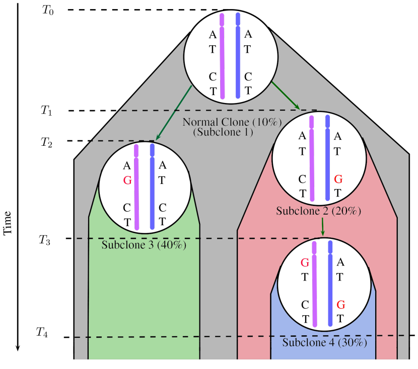
Fig. 2 presents a stylized example of temporal evolution of a tumor, starting from time and evolving until time with the normal clone (subclone ) and three tumor subclones (). Each tumor subclone is marked by two mutation pairs with distinct somatic mutation profiles. In Fig. 2 the true phylogenetic tree is plotted connecting the stylized subclones. The true population frequencies of the subclones are marked in parentheses. In panel (b) subclone genomes, their population frequencies and the phylogenetic relationship are represented by , , and . Next we explain in detail the definition of these parameters.
The entries of report for each subclone the index of the parent subclone (with for the root clone ). Suppose mutation pairs with subclones are present. The subclone phylogeny can be visualized with a rooted tree with nodes. We use a -dimensional parent vector to encode the parent-child relationship of a tree, where means that subclone is the parent of subclone . The parent vector uniquely defines the topology of a rooted tree. We assume that the tumor evolutionary process always starts from the normal clone, indexed by . The normal clone does not have a parent, and we denote it by . For example, the parent vector representation of the subclone phylogeny in Fig. 2 is .

We use the matrix to represent the subclone genotypes. Each column of defines a subclone, and each row of corresponds to a mutation pair. The entry records the genotypes for mutation pair in subclone . Since each subclone has two alleles , and each mutation pair has two loci , the entry is itself a matrix,
where
and
represent mutation pairs of allele and allele , respectively.
That is, in , and index the two alleles and the
two loci, respectively.
Theoretically, each can be any one of the four nucleotide
sequences, A, C, G, T. However, at a single locus, the probability of
having more than two sequences is negligible since it would require
the same locus to be mutated twice throughout the life span of the
tumor, which is extremely unlikely.
Therefore, we assume can only take two possible values,
with (or ) indicating that the corresponding locus has a
mutation (or does not have a mutation) compared to the reference
genome, respectively.
For example, in Fig. 2, we have mutation pairs
and subclones.
For mutation pair in subclone , the allele
harbors no mutation, while the allele has a mutation at the
first locus , which translates to (writing
00 as a shorthand for , etc.).
Altogether, can take possible
values . Since
we do not have phasing information across mutation pairs, the
values having mirrored columns lead to exactly the same data
likelihood and thus are indistinguishable.
This reduces the list of possible values of to the
values,
, ,
, , , , , , and .
We assume that the normal subclone has no mutation, for
all , indicating all mutations are somatic.
Finally, we introduce notation for mixing proportions . Suppose tissue samples are dissected from the same patient. We assume that the samples are admixtures of subclones, each sample with a different set of mixing proportions (population frequencies). We use a matrix to record the proportions, where represents the population frequencies of subclone in sample , and . The proportions denotes the proportion of normal cells contamination in sample (and later we will still add a weight for a background clone ).
2.2 Sampling Model
Let be a matrix with representing read depth for mutation pair in sample . It records the number of times any locus of the mutation pair is covered by sequencing reads (see Fig. 1). Let be a specific short read where index the two loci in a mutation pair, . We use (or ) to denote a variant (reference) sequence at the read, compared to the reference genome. An important feature of the data is that read may overlap in only one locus. We use to represent the missing other sequence on the read. Reads that do not overlap with either of the two loci are not included in the model as they do not contribute any information about the mutation pair. In summary, can take possible values,
Among all reads, let be the number of short reads having genotype . E.g., in Fig. 1 out of a total of reads, we have and .
We assume a multinomial sampling model for the observed read counts
| (1) |
where is the probability of observing a short read with genotype . Next we link with the underlying subclone structures.
For a short read , depending on whether it covers both loci or only one locus, we consider three cases: (i) a read covers both loci, taking values (complete read); (ii) a read covers the second locus, taking values (left missing read); and (iii) a read covers the first locus, taking values (right missing read). Let denote the probabilities of observing a short read of type (i), (ii) and (iii), respectively. Conditional on cases (i), (ii) or (iii), let be the conditional probability of observing . We have , , and . We assume non-informative missingness and do not make inference on ’s. So they remain constants in the likelihood.
We express in terms of and based on the following generative model in three steps. Consider a sample . To generate a short read, we first select a subclone with probability (step 1). Next we select with probability one of the two alleles (step 2). Finally, we record the read , or , corresponding to the chosen allele (step 3). In the case of left (or right) missing locus we observe , or (or or ), corresponding to the observed locus of the chosen allele. Reflecting steps 2 and 3, we denote the probability of observing a short read from subclone characterized by by
| (2) |
with the understanding that for missing reads. Implicit in (2) is the restriction , depending on the arguments. Finally, proceeding as in step 1 we use the conditional probabilities to obtain the marginal probability of observing a short read from the tumor sample with subclones with cellular proportions as
| (3) |
The first term in Eq. 3 states that the probability of observing a short read with genotype is a weighted sum of the ’s across all the subclones.
The last term introduces the notion of a background subclone, indexed as and without biological meaning, to account for noise and artifacts in the NGS data (sequencing errors, mapping errors, etc.), and also for tiny subclones that are not detectable given the sequencing depth. In (3), stands for the probability of observing due to this random noise. We assume the random noise does not differ across different mutation pairs, thus does not have an index . Note that .
Finally, we note that if desired, it is straightforward to incorporate data for marginal SNV reads in the sampling model by treating such reads as, for example, right missing reads, i.e. . In this case, , and the multinomial sampling model reduces to a binomial model. The addition of marginal SNV counts does not typically improve inference. See more details in Zhou et al. (2017).
2.3 Prior Model
We construct a hierarchical prior model, starting with , then a prior on the tree for a given number of nodes, , and finally a prior on the subclonal genotypes given the phylogenetic tree . We assume a geometric prior for the number of subclones, , . Conditional on , the prior on the tree, is as in Chipman et al. (1998). For a tree with nodes, we let
where is the depth of node , or the number of generations between node and the normal subclone . The prior penalizes deeper trees and thus favors parsimonious representation of subclonal structure.
Conditional on we define a prior for . The subclone genotype matrix can be thought of as a feature allocation for categorical matrices. The mutation pairs are the objects, and the subclones are the latent features chosen by the objects. Each feature has 10 categories corresponding to the different genotypes. Given the construction of the subclone genotype matrix needs to introduce dependence across features to respect the assumed phylogeny. We construct a prior for based on the following generative model. We start from a normal subclone denoted by . Now consider a subclone and defined by . The subclone preserves all mutations from its parent , but also gains a Poisson number of new mutations. We assume the new mutations happen randomly at the unmutated loci of the parent subclone. A formal description of prior of follows.
For a subclone , let denote the number of mutations in mutation pair , and let denote the mutation pairs in subclone that have less than four mutations. Let denote the number of new mutations that mutation pair gains compared to its parent, and let . We assume (i) The child subclone should acquire at least one additional mutation compared with its parent (otherwise subclone would be identical to its parent ). (ii) If the parent has already acquired all four mutations for a given , then the child can not gain any more new mutation. That is, if , then . (iii) Each mutation pair can gain at most one additional mutation in each generation, . Based on these assumptions, given a parent subclone , we construct a child subclone as follows. Let be the set of mutation pairs in subclone where new mutations are gained. Let denote a uniformly chosen subset of of size , and let represent a Poisson distribution with mean , truncated to . We assume
| (4) |
The lower bound and upper bound of the truncated Poisson reflect assumptions (i) and (ii) respectively. Also, Eq. 4 implicitly captures assumption (iii).
Next, for a mutation pair that gains one new mutation, we assume the new mutation randomly arises in any of the unmutated loci in the parent subclone. Let , and let denote a uniform distribution over the set . We first choose
and then set . So we have
The prior construction is completed with a prior for and . We design the prior of in such a manner that we could put an informative prior for if a reliable estimate for tumor purity is available based on some prior bioinformatics pipeline (e.g. Van Loo et al. (2010); Carter et al. (2012)). Recall that is the normal subclone, i.e., is the normal subclone proportion (or 1 minus tumor purity), and that . We assume a Beta-Dirichlet prior on such that,
where . We set as is only a correction term to account for background noise and model mis-specification term.
Finally, to specify a prior for we consider complete reads, left missing reads and right missing reads separately and assume , , and .
3 Posterior Inference
Let denote the unknown parameters except for the number of subclones and the tree . Markov chain Monte Carlo (MCMC) simulation from the posterior is used to implement posterior inference. Gibbs sampling transition probabilities are used to update , and Metropolis-Hastings transition probabilities are used to update and . For example, we update by row with
where is a row of satisfying the phylogeny .
Since the posterior distribution is expected to be highly multi-modal, we utilize parallel tempering [Geyer (1991)] to improve the mixing of the chain. Specifically, we use OpenMP parallel computing API [Dagum and Menon (1998)] in C++, to implement a scalable parallel tempering algorithm.
Updating and is more difficult. In general, posterior MCMC on tree structures can be very challenging to implement [Chipman et al. (1998); Denison et al. (1998)]. However, the problem here is manageable since plausible numbers for constrain to moderately small trees. We assume that the number of nodes is a priori restricted to . Conditional on the number of subclones , the number of possible tree topologies is finite. Let denote the (discrete) sample space of . Updating the values of involves trans-dimensional MCMC. At each iteration, we propose new values for from a uniform proposal, .
In order to search the space for the number of subclones and trees that best explain the observed data, we follow a similar approach as in Lee et al. (2015); Zhou et al. (2017) (motivated by fractional Bayes’ factor in O’Hagan (1995)) that splits the data into a training set and a test set. Recall that represents the read counts data. We split into a training set with , and a test set with . Let be the posterior evaluated on the training set only. We use in two instances. First, is used as an informative prior instead of the original prior , and second, is used as a proposal distribution for , . Finally, the acceptance probability of proposal is evaluated on the test set. Importantly, in the acceptance probability the (intractable) normalization constant of cancels out, making this approach computationally feasible.
Here we use as an informative proposal distribution for to achieve a better mixing Markov chain Monte Carlo simulation with reasonable acceptance probabilities. Without the use of an informative proposal, the proposed new tree is almost always rejected because the multinomial likelihood with the large sample size is very peaked. Under the modified prior , the resulting conditional posterior on remains entirely unchanged, [Zhou et al. (2017)].
The described uniform tree proposal is in contrast to usual search algorithms for trees that generate proposals from neighboring trees. Such algorithms have the important drawback that they quickly gravitate towards a local mode and then get stuck. A possible approach to addressing this problem is to repeatedly restart the algorithm from different starting trees. See Chipman et al. (1998) for more details. Our uniform tree proposal combined with the data splitting scheme is another way to mitigate this challenge, efficiently searching the tree space while keeping a reasonable acceptance probability.
All posterior inference is contained in the posterior distribution for and . For example, the marginal posterior distribution of and gives updates posterior probabilities for all possible values of and . But it is still useful to report point estimates. We use the posterior modes as point estimates for , and conditional on and , we use the maximum a posteriori (MAP) estimator as an estimation for the other parameters. The MAP is approximated as the MCMC sample with highest posterior probability. Let be a set of MCMC samples of , and
We report point estimates as , and .
4 Simulation Studies
We carried out three simulation studies to assess the performance of TreeClone. We simulate multiple datasets with different number of subclones (), number of samples (), average read depths () and left and right missing rates () to test the performance of the proposed model in different scenarios. In all simulation studies, we generate hypothetical read count data for dozens of mutation pairs ( for simulations 1 and 2, and for simulation 3), which is a typical number of mutation pairs in a real tumor sample.
4.1 Simulation 1, Convergence Diagnostic and Sensitivity Analysis
Simulation 1(a)
We first validate TreeClone on 9 simulated datasets, one for each combination of and average read depth . For all 9 datasets, we consider samples and mutation pairs. We randomly generate the phylogenetic tree and the genotype matrix from the prior model. The subclone proportions are simulated from , , for , and , respectively. Here stands for a random permutation of . The noise fractions are generated from the prior with . We mimic a typical rate of left (or right) missing reads by setting , for all and . The read depth is generated from a negative-binomial distribution, , to reflect the over-dispersion of read depth in sequencing data. We fix and such that and for , and . Finally, the read counts are simulated from the multinomial sampling model (1).
We fit the model with the following hyperparameters: , , , , , where the values of and imply mild penalty for deep and bushy trees [Chipman et al. (1998)], and other hyperparameters are default non-informative choices. We set for given as a non-informative prior choice and set to express our prior belief that about half of the mutations occur uniformly at each generation. We use and as the range of for computational efficiency. In principle can be any finite number. However, the size of the tree space grows exponentially with , so that the time needed for achieving a good mixing Markov chain grows exponentially. We set the training set fraction (in the trans-dimensional MCMC implementation) to , which we found to performs well in all simulation studies. We run a total of 8000 MCMC iterations. Discarding the first 3000 draws as initial burn-in, we have a Monte Carlo sample with 5000 posterior draws.
We evaluate the performance of TreeClone in estimating the number of subclones , phylogeny , genotype and subcone proportions . To this end, we define the reconstruction error rates , ,
and , similar to Marass et al. (2017). Here is a permutation of columns of to account for label-switching of subclones, and the same permutation is imposed on columns of . The simulation results are summarized in Table 1. For all 9 simulated datasets TreeClone nicely recovers the truth and attains reasonably low reconstruction errors.
| 3 | 4 | 5 | |
|---|---|---|---|
| 50 | 0, 0, 0.00, 0.09 | 0, 0, 0.03, 0.07 | 0, 0, 0.07, 0.06 |
| 200 | 0, 0, 0.00, 0.15 | 0, 0, 0.00, 0.09 | 0, 0, 0.00, 0.05 |
| 1000 | 0, 0, 0.00, 0.14 | 0, 0, 0.00, 0.10 | 0, 0, 0.00, 0.08 |
To assess the convergence of the MCMC algorithm, for each simulated dataset we run the algorithm three times with different random seeds. We use the log-posterior values to calculate a potential scale reduction factor (PSRF) [Gelman and Rubin (1992)] for the three Markov chains. A PSRF close to 1 indicates convergence of the Markov chain to the target distribution. The results are reported in Table 2. Next, to assess the identifiability of the parameters in the TreeClone model, we calculate frequentist coverage probabilities of posterior credible intervals for . The results are shown as the second entry in each cell of Table 2.
| 3 | 4 | 5 | |
|---|---|---|---|
| 50 | 1.06, | 1.08, | 1.33, |
| 200 | 1.13, | 1.04, | 1.38, |
| 1000 | 1.05, | 1.11, | 3.72, |
Simulation 1(b)
Next, we vary average read depth and . Again we simulate 9 datasets, one for each combination of and with and . We assume the same genotype matrix for all the 9 datasets with subclones and mutation pairs. The parameters are generated from the prior model, and is generated from , as in simulation 1(a).
| 1 | 3 | 5 | |
|---|---|---|---|
| 50 | 0, 0, 0.29, 0.05 | 0, 0, 0.11, 0.09 | 0, 0, 0.03, 0.08 |
| 200 | 0, 0, 0.16, 0.04 | 0, 0, 0.01, 0.07 | 0, 0, 0.00, 0.08 |
| 1000 | 0, 0, 0.13, 0.02 | 0, 0, 0.00, 0.12 | 0, 0, 0.00, 0.10 |
The simulation results are summarized in Table 3. Even with only one sample and low read depth, TreeClone can reliably estimate and (although it does not perfectly recover due to the limited amount of data).
Simulation 1(c)
Finally, we assess sensitivity with respect to the rates of left and right missing mutation pairs and . Missingness is simply due to the length of a short read is not long enough to cover both loci in a mutation pair. Thus, missingness is non-informative, and we assume in the simulation for simplicity. We simulate 5 datasets with missing rates , , , and . The extreme case implies that no complete mutation pair reads are recorded. For all the 5 datasets, we consider samples and average read depth , and we assume the same genotype with subclones and mutation pairs. The parameters are generated from the prior model as in simulation 1(a) and (b). The simulation results are summarized in Table 4. TreeClone maintains high reconstruction accuracy across all scenarios.
| 0, 0, 0.00, 0.08 | 0, 0, 0.00, 0.09 | 0, 0, 0.00, 0.08 | 0, 0, 0.00, 0.07 | 0, 0, 0.12, 0.07 |
Using only marginal SNVs
We consider another simulation assuming that we observe only marginal SNVs that are not phased. We treat the marginal SNVs as right missing reads, i.e. and . We simulate one dataset under this scenario. The reconstruction errors are . The number of subclones and phylogenetic tree are correctly identified. The genotype reconstruction error is high because the data do not provide any information for inferring the unobserved locus for all , and . For a fair comparison we re-define . The re-defined reconstruction error is .
4.2 Simulation 2 and comparison with alternatives
In the second simulation study, we compare the performance of TreeClone with existing methods. We consider sample, which is the case for most real-world tumor cases (due to the challenge in obtaining multiple samples from a patient). In practice we notice that methods using only marginal SNV data find it hard to identify branching in a phylogenetic tree. We use this simulation to illustrate the information gain by using mutation pairs data.
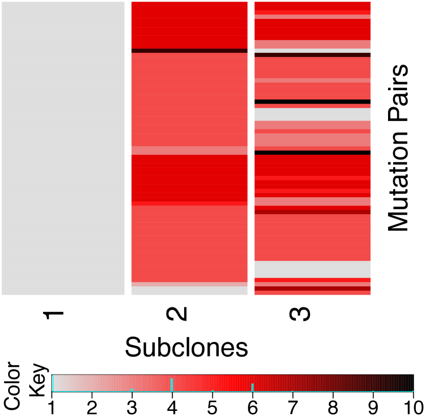
We consider mutation pairs and assume a simulation truth with latent subclones with a true phylogenetic tree as
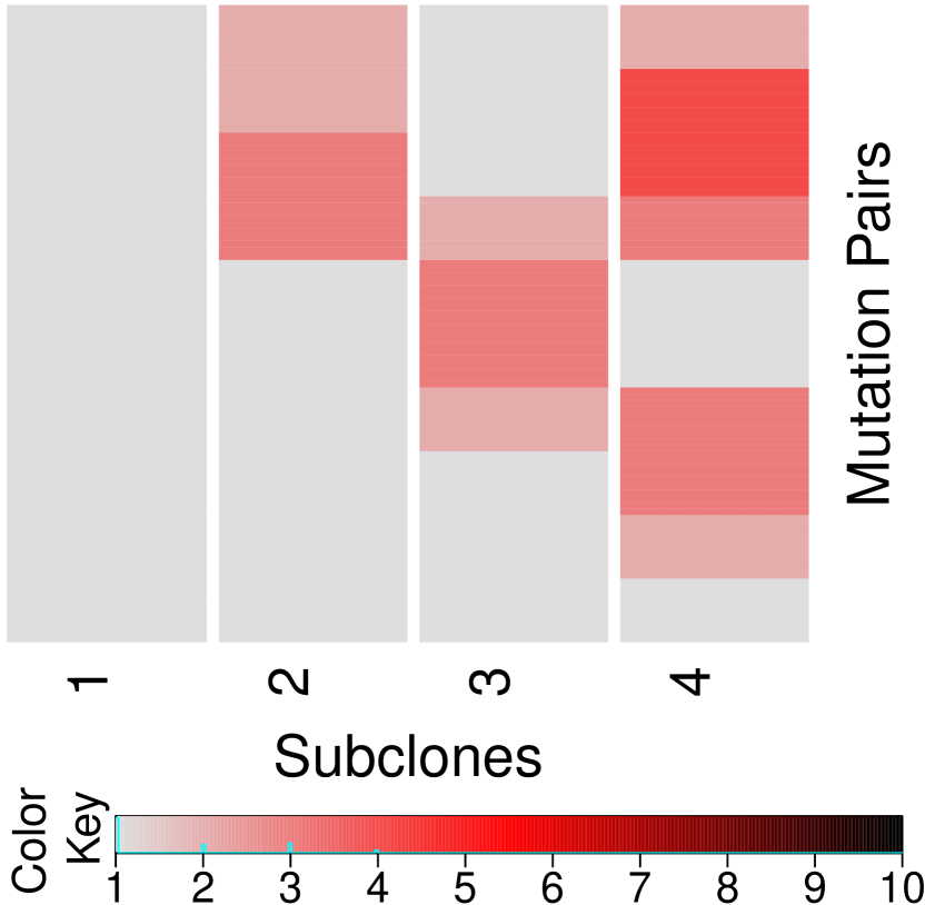
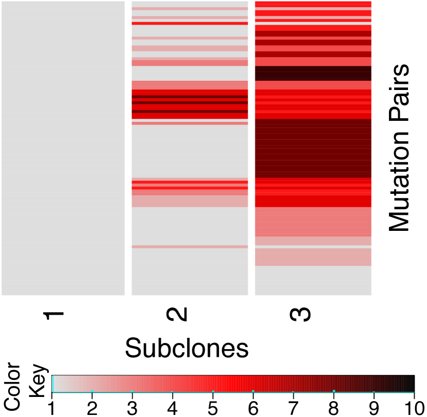
Fig. 3(a) shows the true underlying subclonal genotypes. We use a heatmap to show the subclone matrix , where colors from light gray to red to black are used to represent genotypes to . The subclone weights are simulated from . For the single sample in this simulation we get , , , , . We generate from the prior model with , and we set , for all and . We generate the read depth with and .
The hyperparameters are set as in Simulation 1. To explore a larger tree space, we set , run a total of 13000 MCMC iterations and discard the first 3000 draws as initial burn-in.
Posterior inference is summarized in Fig. 3(b, c). Fig. 3(c) shows the top three tree topologies and corresponding posterior probabilities. The posterior mode recovers the true phylogeny. Fig. 3(b) shows the estimated genotypes conditional on the posterior modes . Some mismatches are due to the single sample and limited read depth. The estimated subclone proportions are , , , , , which agrees with the truth.
| Tree topology | Prob. |
|---|---|
| 0.26 | |
| 0.19 | |
| 0.07 |
Comparison with alternatives
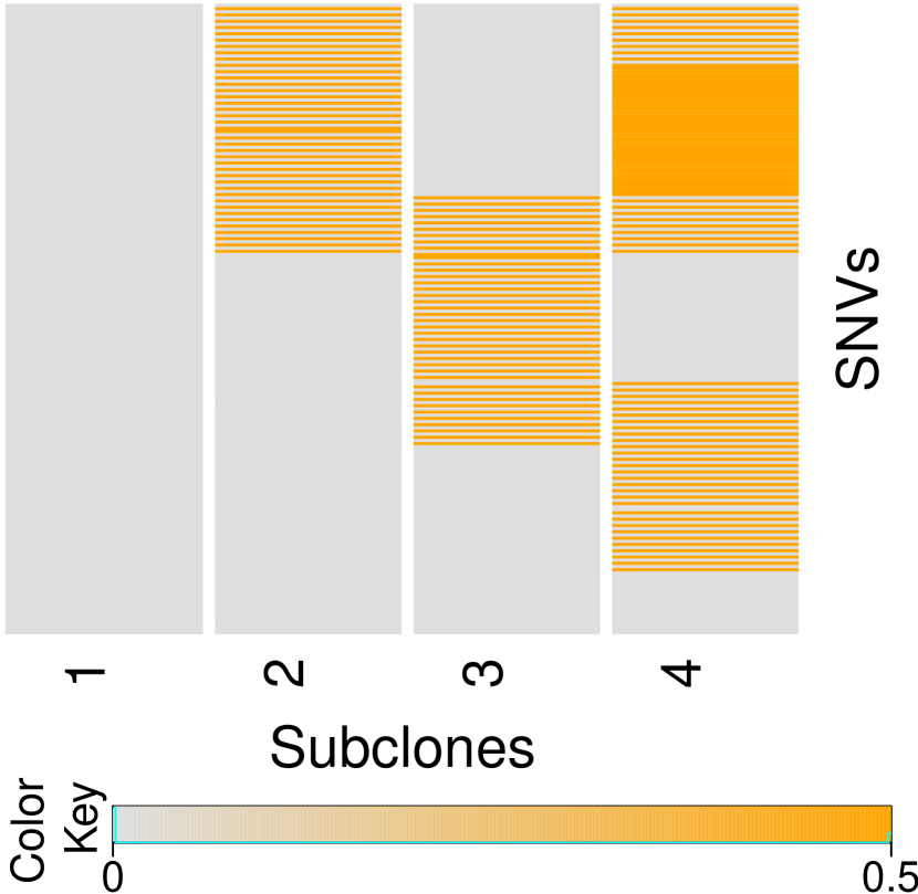
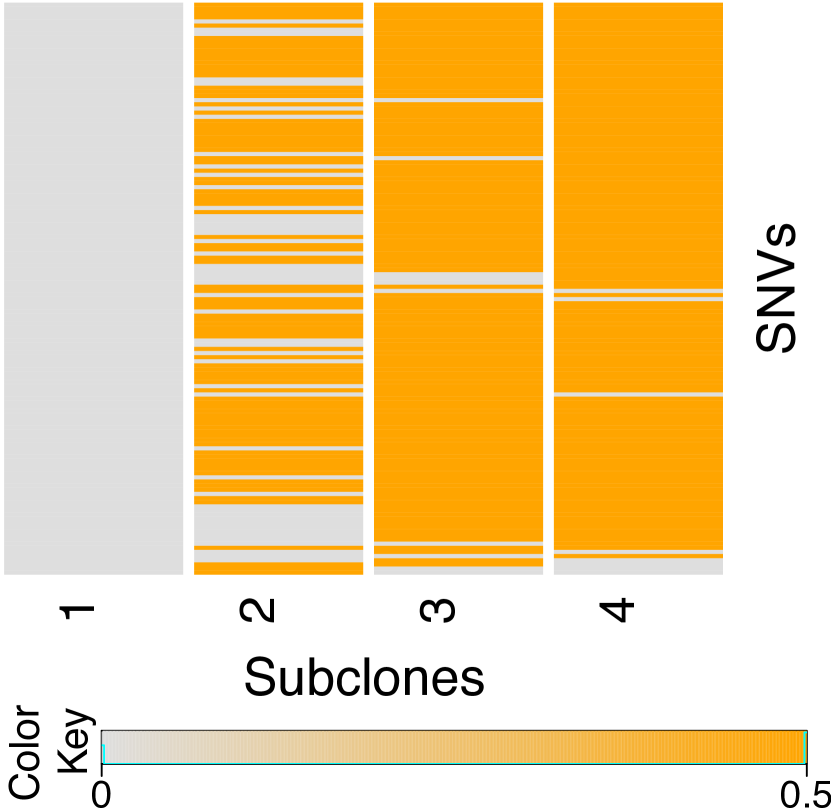
There is no other subclone calling method based on paired-end read data that also infers phylogeny. We therefore compare with other similar model-based approaches. In particular, we use Cloe [Marass et al. (2017)], PhyloWGS [Jiao et al. (2014); Deshwar et al. (2015)] and PairClone [Zhou et al. (2017)] for inference with the same simulated data. Cloe and PhyloWGS infer phylogeny but take marginal SNV data as input. For these methods we therefore discard the phasing information in mutation pairs and only record marginal mutation counts for SNVs. The simulation truth for Cloe and PhyloWGS is shown in Fig. 4(a). The orange color means a heterozygous mutation at the corresponding SNV locus. PairClone takes the same mutant read counts and read depths for mutation pairs as input but uses a different probability model that does not allow to infer the phylogenetic tree.
Cloe infers clonal genotypes and phylogeny based on a similar feature allocation model. We run Cloe with the default hyperparameters for the same number of 13000 iterations with the first 3000 draws as initial burn-in. Based on the MAP estimate (over ), Cloe reports subclones with phylogeny , and the subclone genotypes are shown in Fig. 4(b) with subclone proportions , , .
PhyloWGS, on the other hand, infers clusters of mutations and phylogeny. One can then make phylogenetic analysis to conjecture subclones and genotypes. Let denote the fraction of cells with a variant allele at locus . The ’s are latent quantities related to the observed VAF for each SNV. PhyloWGS infers the phylogeny by clustering SNVs with matching ’s under a tree-structured prior for the unique values . In particular, they use the tree-structured stick breaking process (TSSB) [Adams et al. (2010)]. The TSSB implicitly defines a prior on the formation of subclones, including a prior on and the number of novel loci that arise in each subclone (in contrast, TreeClone explicitly defines these model features, allowing easier prior control on and ). We run PhyloWGS with the default hyperparameters and 2500 iterations with a burn-in of 1000 samples. We only consider loci with VAF as for PhyloWGS the other loci do not provide information on clustering. We then report cluster sizes and phylogeny based on MAP estimate. PhyloWGS reports 3 subclones with phylogeny , where 0 refers to the normal subclone, and the numbers in the brackets refer to the cluster sizes and cellular prevalences. The conjectured subclone genotypes are shown in Fig. 4(c), with subclone proportions , , .

Inferences under Cloe and PhyloWGS do not entirely recover the truth. Let denote the new mutations that are gained by subclone . The reason for the failure to recover the simulation truth is probably that the common mutations of subclones 2 and 4 ( with a cellular prevalence of ) have a similar cellular prevalence as the mutations of subclone 3 ( with a cellular prevalence of ). Therefore, Cloe infers that and belong to the same subclone ( and ). Similarly, PhyloWGS clusters and together. Using more informative mutation pairs data, TreeClone can infer that and belong to different subclones. The inclusion of phasing information from the paired-end read data increases statistical power in recovering the underlying structure.
PairClone uses the same mutation pairs data and same sampling model to infer clonal genotypes. However, PairClone uses a finite categorical Indian buffet process prior for , which assumes independence among the subclones and does not infer phylogeny. PairClone infers 3 subclones with genotypes shown in Fig. 4(d). The estimated subclone proportions are , , , similar to Cloe and PhyloWGS’s results. PairClone does not entirely recover the truth, probably because not imposing the tree structure reduces the identifiability of the problem.
Comparison using additional marginal SNVs
An NGS dataset contains many more marginal SNVs than phased mutation pairs. These additional marginal SNVs can be utilized by methods such as Cloe and PhyloWGS. For an illustration of the information gain by using more SNVs, we run Cloe and PhyloWGS with a larger set of SNVs that contains 400 SNVs in addition to the 200 SNVs that are part of the 100 mutation pairs, i.e., a total of 600 SNVs. We assume a genotype matrix , i.e. repeating the rows of three times, and keep the other parameters unchanged from before.
Using 600 SNVs, Cloe infers two subclones with phylogeny and proportions , . PhyloWGS infers three (conjectured) subclones with phylogeny and proportions , , . The results suggest that the additional 400 SNVs do not contribute much information about the branching in the phylogenetic tree.
4.3 Simulation 3
In the third simulation, we evaluate the performance of the proposed approach on multiple samples. We generate the simulated data by mimicking a real-world lung cancer data (see Section 5). Following that dataset, we consider tissue samples and mutation pairs. The simulation truth and are generated by fitting TreeClone on the lung cancer dataset. We get subclones with phylogeny
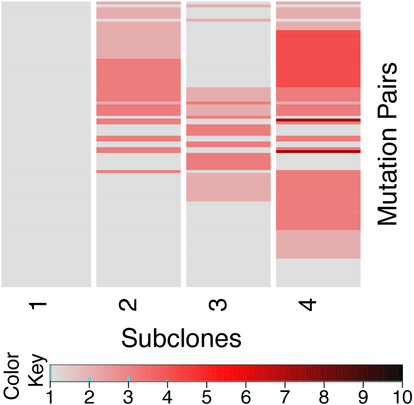
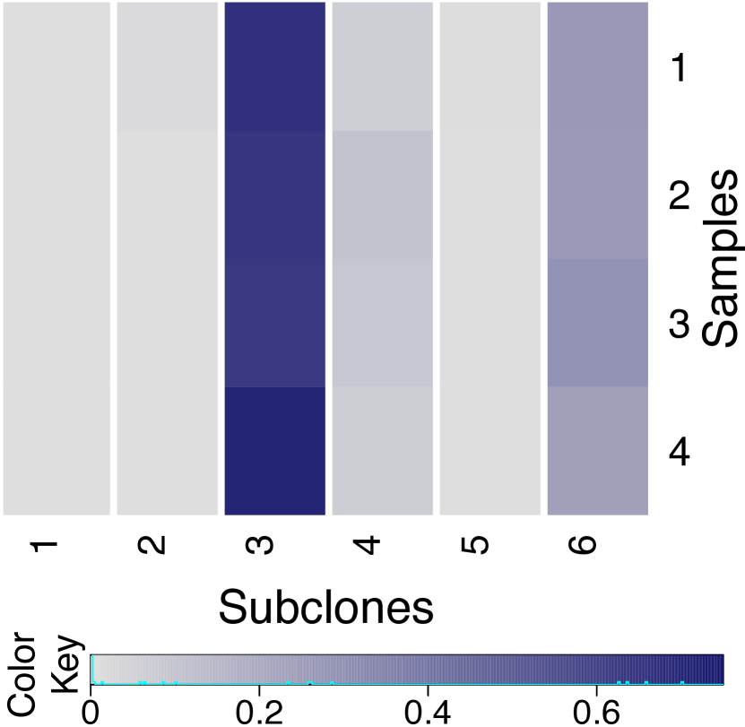
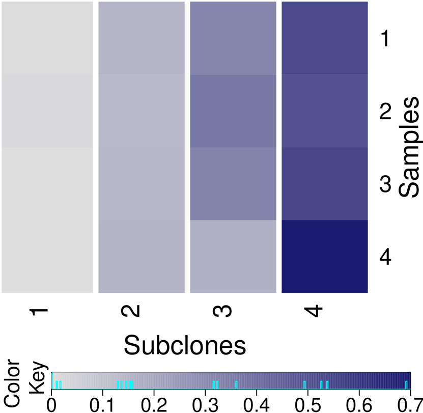
Fig. 5(a, b) shows the simulation truth and in the form of heatmaps, respectively. We show with a light gray to deep blue scale. A darker blue color indicates higher abundance of a subclone in a sample (the proportions of the background subclone are tiny and not shown). Read depths and left and right missing rates are taken to be exactly the same as in the real data. The average read depth is .
The hyperparameters are set as in Simulation 1. To explore a larger tree space, we set , run a total of 30000 MCMC iterations and discard the first 3000 draws as initial burn-in.


| Tree topology | Prob. |
|---|---|
| 0.38 | |
| 0.11 | |
| 0.09 |
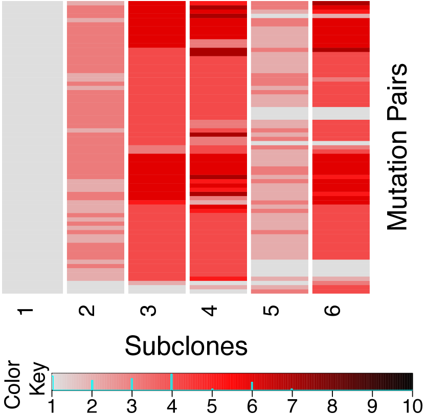
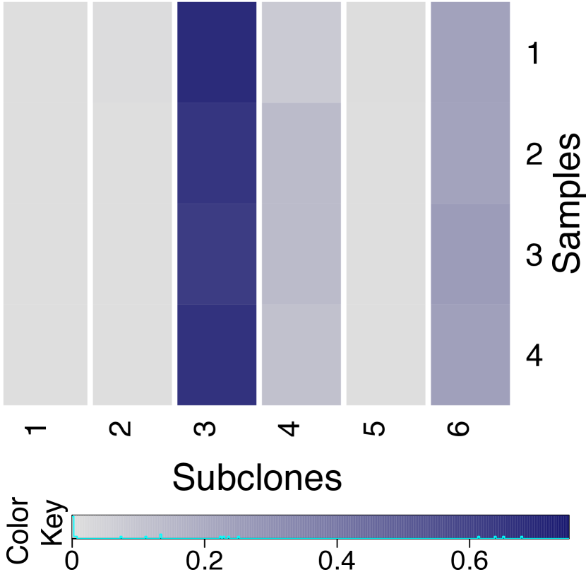
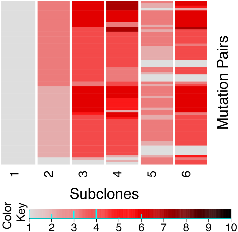
Posterior inference is summarized in Fig. 5(c, d, e). Fig. 5(c) shows the top three tree topologies and corresponding posterior probabilities. The posterior mode recovers the true phylogeny. Fig. 5(d, e) shows the estimated genotypes and subclone proportions conditional on . There are some mismatches for subclones 2, 4 and 5, as they only take small proportions in all the samples ( and for all ). The reconstruction errors are and (considering only subclones 1, 3 and 6 the reconstruction error becomes ).
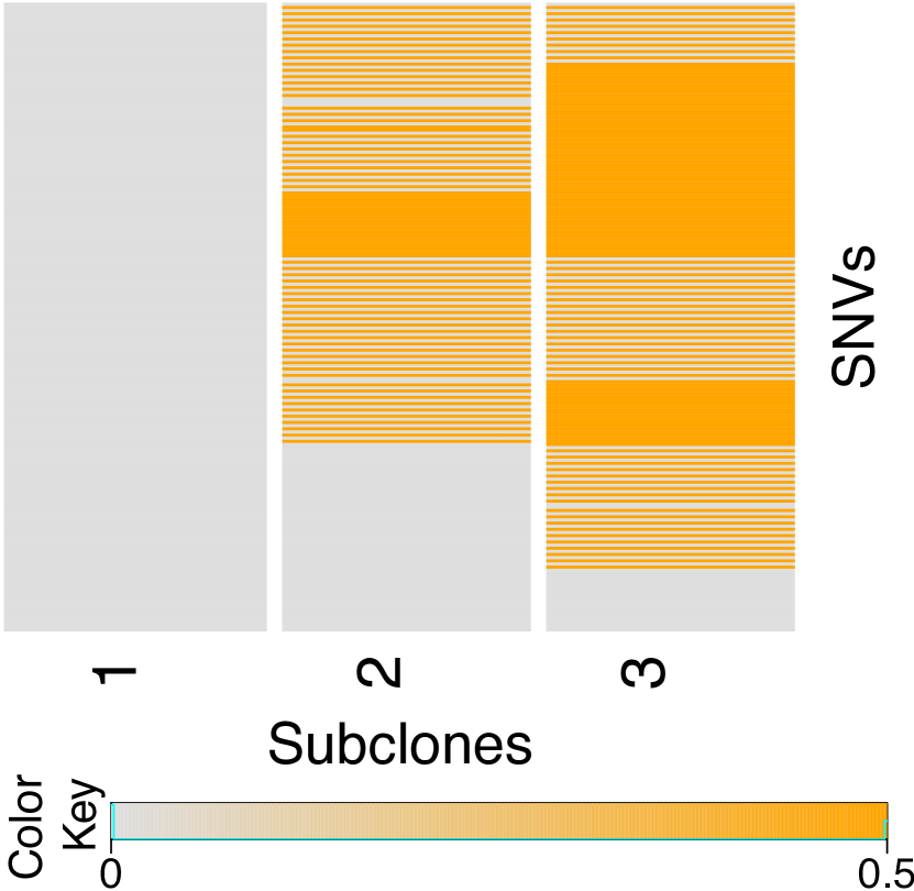
For comparison we again run Cloe, PhyloWGS and PairClone on the same data. Cloe infers three subclones with phylogeny , where Cloe’s subclones 1, 2 and 3 roughly correspond to the true subclones 1, 6 and 3, respectively. Cloe’s result is reasonable since subclones 2, 4 and 5 have small proportions and there is not much statistical power to estimate them. Similar to the definition of , we define for SNVs. Comparing with subclones 1, 6 and 3 we calculate the reconstruction error , indicating good model fit of Cloe. By allowing mutation loss, Cloe infers a linear phylogenetic tree, which is still reasonable. On the other hand, PhyloWGS infers the phylogeny as (details not shown), which approximates but misses some detail in the simulation truth. Finally, PairClone infers three subclones corresponding to the true subclones 1, 3 and 6, shown in Fig. 5(f). PairClone also reasonably recovers the truth but does not infer phylogeny. Comparing with subclones 1, 3 and 6 we calculate the reconstruction error , which is higher than .
5 Lung Dataset
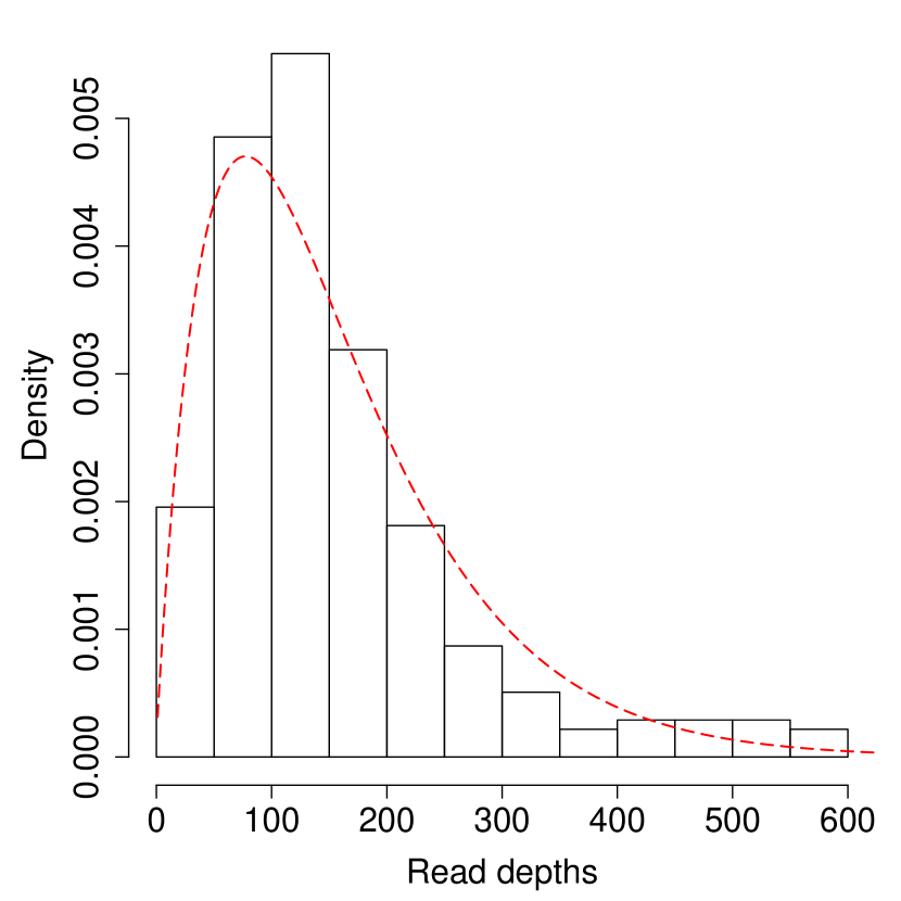
We use whole-exome sequencing (WES) data generated from four () surgically dissected tumor samples taken from a single patient diagnosed with lung adenocarcinoma. DNA is extracted from all four samples and the exome library is sequenced on an Illumina HiSeq 2000 platform in paired-end fashion. Each read is 100 base-pairs long. We use BWA [Li and Durbin (2009)] and GATK’s UniformGenotyper [McKenna et al. (2010)] for mapping and variant calling, respectively. In order to find mutation pair locations along with their genotypes and the number of reads supporting them, we use a bioinformatics tool called LocHap [Sengupta et al. (2016)]. LocHap searches for two or three SNVs that are scaffolded by the same reads. When the scaffolded SNVs, known as local haplotypes, exhibit more than two haplotypes, it is known as local haplotype variant (LHV). Using the individual BAM and VCF files LocHap finds a few hundreds LHVs on average in a WES sample. We select LHVs with two SNVs as we are interested in mutation pairs only. On those LHVs, we run the bioinformatics filters suggested by LocHap to keep the mutation pairs with high calling quality. We focus our analysis in copy number neutral regions. In the end, we get 69 mutation pairs for the sample and record the read count data from the output of LocHap. Figure 6 shows the histograms of read depths, left missing rates and right missing rates. The average read depth, left missing rate and right missing rate are , and , respectively. Simulation 1 showed that with samples TreeClone should provide useful inference with this combination of moderate read depth and left/right missing rates.


We use the same hyperparameters as in Simulation 1. To explore a larger tree space, we set , run a total of 30000 MCMC iterations and discard the first 3000 draws as initial burn-in. Fig. 7(c) shows the top three tree topologies and corresponding posterior probabilities. The posterior mode is
with subclones. Fig. 7(a, b) show the estimated subclone genotypes and cellular proportions , respectively ( are not shown). The rows for are reordered for better display. The cellular proportions of the subclones show strong similarity across the 4 samples, indicating homogeneity of the samples. This is plausible as the samples are dissected from proximal sites. Subclone 1, which is the normal subclone, takes a small proportion in all 4 samples, indicating high purity of the tumor samples. Subclones 2 and 5 are also included in only small proportions. They have almost vanished in the samples. However, as parents of subclones 3, 4 and 6, respectively, they are important for the reconstruction of the subclone phylogeny. Subclones 3, 4 and 6 are the three main subclones. They share a large proportion of common mutations, but each one has some private mutations, consistent with the estimated tree.
Test of fit
Finally, Fig. 7(d) shows a histogram of residuals, where we calculate empirical values and plot the difference . The residuals are centered at zero with little variation, indicating a good model fit. For a more formal goodness-of-fit test, we carried out the Bayesian test proposed in Johnson (2004). Recall that the observations in our case are short reads taking discrete values . We count the number of short reads that fall into each of these categories. Let denote these counts, and let be a posterior sample of . The statistic is defined as
where and is the expected proportion of short reads in category calculated by . Under the null hypothesis of a good model fit the statistic should follow a -distribution with degrees of freedom. Fig. 7(e) shows a quantile-quantile plot of posterior samples of against expected order statistics from a distribution. In addition, find the proportion of posterior samples of exceeding the quantile of a distribution to be 0.054. There is no evidence of a lack of fit.
| Tree topology | Prob. |
|---|---|
| 0.27 | |
| 0.17 | |
| 0.15 |


Cloe and PhyloWGS
For comparison, we run Cloe and PhyloWGS on the same data set with default hyperparameters. Cloe infers four subclones with phylogeny . Fig. 8(a, b) show the estimated genotypes and cellular proportions , respectively. The estimated subclones 2, 3 and 4 under Cloe match with subclones 6, 4 and 3, respectively, under TreeClone. Cloe infers a linear phylogenetic tree since it allows mutation loss. PhyloWGS estimates 6 clusters (and a cluster 0 for normal subclone) of the SNVs with phylogeny
Fig. 8(c) summarizes the cluster sizes and cellular prevalences. In light of the earlier simulation studies we believe that the inference on under TreeClone is more reliable. However, results from Cloe and PhyloWGS confirm that the four samples have similar proportions of all the subclones, indicating little inter-sample heterogeneity. Also, Cloe and PhyloWGS infer very small normal cell proportion, confirming the high tumor purity found by TreeClone. Finally, the same lung cancer dataset was analyzed under PairClone in Zhou et al. (2017). PairClone infers three subclones corresponding to TreeClone’s subclones 1, 3 and 6 and also confirms the 4 tissue samples are highly homogenuous. PairClone gives reasonable result but can not infer phylogeny.
| 1 | 2 | 3 | 4 | |
|---|---|---|---|---|
| 0 (0) | 1.0 | 1.0 | 1.0 | 1.0 |
| 1 (93) | 0.977 | 0.990 | 0.989 | 0.980 |
| 2 (32) | 0.854 | 0.816 | 0.832 | 0.852 |
| 3 (6) | 0.532 | 0.431 | 0.473 | 0.596 |
| 4 (3) | 0.433 | 0.408 | 0.445 | 0.386 |
| 5 (3) | 0.252 | 0.180 | 0.229 | 0.152 |
| 6 (1) | 0.112 | 0.108 | 0.056 | 0.127 |
6 Discussion
In this work, using a tree-based LFAM we infer subclonal genotypes structure for mutation pairs, their cellular proportions and the phylogenetic relationship among subclones. This is the first attempt to generate a subclonal phylogenetic structure using mutation pair data. We show that more accurate inference can be obtained using mutation pairs data compared to using only marginal counts for single SNVs. The model can be easily extended to incorporate more than two SNVs. Another way of extending the model is to encode mutation times inside the length of the edges of phylogenetic tree.
The major motivation for accurate estimation of heterogeneity in tumor is personalized medicine. The next step towards this goal is to use varying estimates of subclonal proportions across patients to drive adaptive treatment allocation.
Currently the heterogeneity is measured mostly with SNV and CNA data. However, structural variants (SVs) like deletion, duplication, inversion, translocation and other large genome rearrangement arguably provide more accurate data for VAF estimation [Fan et al. (2014)], which is the key input for characterizing tumor heterogeneity. Therefore incorporation of SVs into the current model could significantly improve the outcome of tumor heterogeneity analysis. Recently, in Brocks et al. (2014) the authors attempted to explain intratumor heterogeneity in DNA methylation and copy-number pattern by a unified evolutionary process. The current genome centric definition of tumor heterogeneity could be extended by incorporation of methylation, DNA mutation, and RNA expression data in an integromics model.
Finally in the era of big data it is important to factor computation into the research effort, and build efficient computational models that could handle millions of SNVs. Linear response variational Bayes [Giordano et al. (2015)] or MAD-Bayes [Broderick et al. (2013); Xu et al. (2015)] methods could be considered as alternative computational strategies to tackle the problem.
Appendix
Glossary of terms
SNV
A single nucleotide variant or SNV is a DNA sequence variation where one nucleotide is replaced by anther nucleotide. This is very similar to a single nucleotide polymorphism or SNP. In our paper, the term SNV is preferred over SNP because the latter includes an additional interpretation about variants in a population. This means that an SNV could potentially be a SNP but this cannot be determined at the point where the variant is detected in a single sample.
SCNA
Copy number aberration (CNA) is gain or loss of large segments of the genome ranging in size from a few kilobases to a whole chromosomes. Somatic CNA (SCNA) that occurs during the lifetime of an individual is a major contributor to cancer development, particularly for solid tumors.
Short-read
Short DNA sequences produced by the sequencing machine. The range of the read length of a short-read sequencing instrument is between and bp.
Phasing
Phasing helps to identify the copy of the chromosome (paternal or maternal chromosome) to which a particular allele belongs or alternatively, which alleles appear together on the same chromosome. In short-read sequencing, for example, it is difficult to resolve the haplotype of two heterozygous SNPs if they have not been covered by the same read. If you observe A/C and G/T, it is difficult to know whether we have AG and CT or CG and AT.
VAF
Variant allele frequency or VAF is the relative frequency of an alternative allele at a particular genomic locus expressed as a fraction or percentage. The quantity is calculated as the fraction of short-reads overlapping a genomic locus that support the non-reference (mutant/alternate) allele.
Purity
Tumor purity is an essential component in finding tumor heterogeneity. The tumor micro-environment contains other non-cancerous cell types including fibroblasts, immune cells, endothelial cells and normal epithelial cells along with cancer cells. Tumor purity is the proportion of cancer cells in the sample.
Phylogenetic tree
A phylogenetic tree of a tumor sample is a branching diagram or “tree” showing the evolutionary relationships among various subclones that co-exist in the sample.
Subclone calling method
Subclone calling method refers to a computation algorithm that is used to infer the subclonal structure in a tumor sample.
References
- Adams et al. (2010) Adams, R. P., Z. Ghahramani, and M. I. Jordan (2010). Tree-structured stick breaking for hierarchical data. In Advances in neural information processing systems, pp. 19–27.
- Aparicio and Caldas (2013) Aparicio, S. and C. Caldas (2013). The implications of clonal genome evolution for cancer medicine. New England journal of medicine 368(9), 842–851.
- Bafna et al. (2003) Bafna, V., D. Gusfield, G. Lancia, and S. Yooseph (2003). Haplotyping as perfect phylogeny: a direct approach. Journal of Computational Biology 10(3-4), 323–340.
- Bonavia et al. (2011) Bonavia, R., W. K. Cavenee, F. B. Furnari, et al. (2011). Heterogeneity maintenance in glioblastoma: a social network. Cancer research 71(12), 4055–4060.
- Brocks et al. (2014) Brocks, D., Y. Assenov, S. Minner, O. Bogatyrova, R. Simon, C. Koop, C. Oakes, M. Zucknick, D. B. Lipka, J. Weischenfeldt, et al. (2014). Intratumor DNA methylation heterogeneity reflects clonal evolution in aggressive prostate cancer. Cell reports 8(3), 798–806.
- Broderick et al. (2013) Broderick, T., B. Kulis, and M. Jordan (2013). MAD-Bayes: MAP-based asymptotic derivations from Bayes. In Proceedings of The 30th International Conference on Machine Learning, pp. 226–234.
- Carter et al. (2012) Carter, S. L., K. Cibulskis, E. Helman, A. McKenna, H. Shen, T. Zack, P. W. Laird, R. C. Onofrio, W. Winckler, B. A. Weir, et al. (2012). Absolute quantification of somatic DNA alterations in human cancer. Nature biotechnology 30(5), 413–421.
- Chipman et al. (1998) Chipman, H. A., E. I. George, and R. E. McCulloch (1998). Bayesian CART model search. Journal of the American Statistical Association 93(443), 935–948.
- Dagum and Menon (1998) Dagum, L. and R. Menon (1998). OpenMP: an industry standard API for shared-memory programming. Computational Science & Engineering, IEEE 5(1), 46–55.
- Denison et al. (1998) Denison, D. G. T., B. K. Mallick, and A. F. M. Smith (1998). A Bayesian CART algorithm. Biometrika 85(2), pp. 363–377.
- Deshwar et al. (2015) Deshwar, A. G., S. Vembu, C. K. Yung, G. H. Jang, L. Stein, and Q. Morris (2015). PhyloWGS: reconstructing subclonal composition and evolution from whole-genome sequencing of tumors. Genome biology 16(1), 35.
- Fan et al. (2014) Fan, X., W. Zhou, Z. Chong, L. Nakhleh, and K. Chen (2014). Towards accurate characterization of clonal heterogeneity based on structural variation. BMC bioinformatics 15(1), 1.
- Fischer et al. (2014) Fischer, A., I. Vázquez-García, C. J. Illingworth, and V. Mustonen (2014). High-Definition Reconstruction of Clonal Composition in Cancer. Cell Reports 7, 1740–1752.
- Gelman and Rubin (1992) Gelman, A. and D. B. Rubin (1992). Inference from iterative simulation using multiple sequences. Statistical science, 457–472.
- Geyer (1991) Geyer, C. J. (1991). Markov chain Monte Carlo maximum likelihood. Interface Foundation of North America.
- Giordano et al. (2015) Giordano, R. J., T. Broderick, and M. I. Jordan (2015). Linear response methods for accurate covariance estimates from mean field variational Bayes. In Advances in Neural Information Processing Systems, pp. 1441–1449.
- Jiao et al. (2014) Jiao, W., S. Vembu, A. G. Deshwar, L. Stein, and Q. Morris (2014). Inferring clonal evolution of tumors from single nucleotide somatic mutations. BMC bioinformatics 15(1), 35.
- Johnson (2004) Johnson, V. E. (2004). A bayesian test for goodness-of-fit. The Annals of Statistics 32(6), 2361–2384.
- Lee et al. (2015) Lee, J., P. Müller, K. Gulukota, Y. Ji, et al. (2015). A Bayesian feature allocation model for tumor heterogeneity. The Annals of Applied Statistics 9(2), 621–639.
- Li and Durbin (2009) Li, H. and R. Durbin (2009). Fast and accurate short read alignment with Burrows–Wheeler transform. Bioinformatics 25(14), 1754–1760.
- Marass et al. (2017) Marass, F., F. Mouliere, K. Yuan, N. Rosenfeld, and F. Markowetz (2017). A phylogenetic latent feature model for clonal deconvolution. The Annals of Applied Statistics 10(4), 2377–2404.
- Marusyk et al. (2012) Marusyk, A., V. Almendro, and K. Polyak (2012). Intra-tumour heterogeneity: a looking glass for cancer? Nature Reviews Cancer 12(5), 323–334.
- McKenna et al. (2010) McKenna, A., M. Hanna, E. Banks, A. Sivachenko, K. Cibulskis, A. Kernytsky, K. Garimella, D. Altshuler, S. Gabriel, M. Daly, et al. (2010). The Genome Analysis Toolkit: a MapReduce framework for analyzing next-generation DNA sequencing data. Genome research 20(9), 1297–1303.
- Miller et al. (2014) Miller, C. A., B. S. White, N. D. Dees, M. Griffith, J. S. Welch, O. L. Griffith, R. Vij, M. H. Tomasson, T. A. Graubert, M. J. Walter, et al. (2014). SciClone: inferring clonal architecture and tracking the spatial and temporal patterns of tumor evolution. PLoS computational biology 10(8), e1003665.
- Miller et al. (2008) Miller, K. T., T. Griffiths, and M. I. Jordan (2008). The phylogenetic Indian buffet process: a non-exchangeable nonparametric prior for latent features. In Proc. UAI.
- Nik-Zainal et al. (2012) Nik-Zainal, S., P. Van Loo, D. C. Wedge, L. B. Alexandrov, C. D. Greenman, K. W. Lau, K. Raine, D. Jones, J. Marshall, M. Ramakrishna, et al. (2012). The life history of 21 breast cancers. Cell 149(5), 994–1007.
- Nowell (1976) Nowell, P. C. (1976). The clonal evolution of tumor cell populations. Science 194(4260), 23–28.
- O’Hagan (1995) O’Hagan, A. (1995). Fractional Bayes factors for model comparison. Journal of the Royal Statistical Society. Series B 57, 99–138.
- Roth et al. (2014) Roth, A., J. Khattra, D. Yap, A. Wan, E. Laks, J. Biele, G. Ha, S. Aparicio, A. Bouchard-Côté, and S. P. Shah (2014). PyClone: statistical inference of clonal population structure in cancer. Nature methods 11(4), 396–398.
- Schwarz et al. (2015) Schwarz, R. F., C. K. Ng, S. L. Cooke, S. Newman, J. Temple, A. M. Piskorz, D. Gale, K. Sayal, M. Murtaza, P. J. Baldwin, et al. (2015). Spatial and temporal heterogeneity in high-grade serous ovarian cancer: a phylogenetic analysis. PLoS medicine 12(2), e1001789.
- Sengupta et al. (2016) Sengupta, S., K. Gulukota, Y. Zhu, C. Ober, K. Naughton, W. Wentworth-Sheilds, and Y. Ji (2016). Ultra-fast local-haplotype variant calling using paired-end DNA-sequencing data reveals somatic mosaicism in tumor and normal blood samples. Nucleic acids research 44(3), e25–e25.
- Sengupta et al. (2015) Sengupta, S., J. Wang, J. Lee, P. Müller, K. Gulukota, A. Banerjee, and Y. Ji (2015). BayClone: Bayesian nonparametric inference of tumor subclones using NGS data. In Proceedings of The Pacific Symposium on Biocomputing (PSB), Volume 20, pp. 467–478.
- Van Loo et al. (2010) Van Loo, P., S. H. Nordgard, O. C. Lingjærde, H. G. Russnes, I. H. Rye, W. Sun, V. J. Weigman, P. Marynen, A. Zetterberg, B. Naume, et al. (2010). Allele-specific copy number analysis of tumors. Proceedings of the National Academy of Sciences 107(39), 16910–16915.
- Xu et al. (2015) Xu, Y., P. Müller, Y. Yuan, K. Gulukota, and Y. Ji (2015). MAD Bayes for tumor heterogeneity – feature allocation with exponential family sampling. Journal of the American Statistical Association 110(510), 503–514.
- Zare et al. (2014) Zare, H., J. Wang, A. Hu, K. Weber, J. Smith, D. Nickerson, C. Song, D. Witten, C. A. Blau, and W. S. Noble (2014). Inferring clonal composition from multiple sections of a breast cancer. PLoS computational biology 10(7), e1003703.
- Zhou et al. (2017) Zhou, T., P. Müller, S. Sengupta, and Y. Ji (2017). PairClone: A Bayesian subclone caller based on mutation pairs. arXiv preprint arXiv:1702.07465.