Disentangling and modeling interactions in fish with burst-and-coast swimming

Abstract

We combine extensive data analyses with a modeling approach to measure, disentangle, and reconstruct the actual functional form of interactions involved in the coordination of swimming in Rummy-nose tetra (Hemigrammus rhodostomus). This species of fish performs burst-and-coast swimming behavior that consists of sudden heading changes combined with brief accelerations followed by quasi-passive, straight decelerations. We quantify the spontaneous stochastic behavior of a fish and the interactions that govern wall avoidance and the attraction and alignment to a neighboring fish, the latter by exploiting general symmetry constraints for the interactions. In contrast with previous experimental works, we find that both attraction and alignment behaviors control the reaction of fish to a neighbor. We then exploit these results to build a model of spontaneous burst-and-coast swimming and interactions of fish, with all parameters being estimated or directly measured from experiments. This model quantitatively reproduces the key features of the motion and spatial distributions observed in experiments with a single fish and with two fish. This demonstrates the power of our method that exploits large amounts of data for disentangling and fully characterizing the interactions that govern collective behaviors in animals groups. Moreover, we introduce the notions of “dumb” and “intelligent” active matter and emphasize and clarify the strong differences between them.

I Introduction

The study of physical or living self-propelled particles – active matter – has certainly become a booming field, notably involving biologists and physicists, often working together. Physical examples of active matter include self-propelled Janus colloids AM1 ; AM2 ; AM3 ; AM4 ; AM5 ; AM6 ; AM7 ; AM8 , vibrated granular matter AM9 ; AM10 ; AM11 , or self-propulsion mediated by hydrodynamical effects AM12 ; AM13 , whereas biological examples are obviously ubiquitous: bacteria, cells, and simply speaking, most animals. In both physical and biological contexts, active matter can organize into rich collective phases. For instance, fish schools can be observed in a disordered swarming phase, or ordered schooling and vortex/milling phases Tunstrom2013 ; Calovi2014 .

Yet, there are important difference between “dumb” and “intelligent” active matter (see the Appendix for a more formal definition and discussion). For the former class, which concerns most physical self-propelled particles, but also, in some context, living active matter, interactions with other particles or obstacles do not modify the intrinsic or “desired” velocity of the particles but exert forces whose effect adds up to its intrinsic velocity. Intelligent active matter, like fish, birds, or humans, can also interact through physical forces (a human physically pushing an other one or bumping into a wall) but mostly interact through “social forces”. For instance, a fish or a human wishing to avoid a physical obstacle or an other animal will modify its intrinsic velocity in order to never actually touch it. Moreover, a physical force applied to an intelligent active particle, in addition to its direct impact, can elicit a response in the form of a change in its intrinsic velocity (for instance, a human deciding to escape or resist an other human physically pushing her/him). Social forces strongly break the Newtonian law of action and reaction: a fish or a human avoiding a physical obstacle obviously does not exert a contrary force on the obstacle. In addition, even between two animals 1 and 2, the force exerted by 1 on 2 is most often not the opposite of the force exerted by 2 on 1, since social forces commonly depend on stimuli (vision, hearing…) associated to an anisotropic perception: a human will most often react more to another human ahead than behind her/him. Similarly, social forces between two fish or two humans will also depend on their relative velocities or orientations: the need to avoid an other animal will be in general greater when a collision is imminent than if it is unlikely, due to the velocity directions.

Hence, if the understanding of the social interactions that underlie the collective behavior of animal groups is a central question in ethology and behavioral ecology Camazine2001 ; Giardina2008 , it has also a clear conceptual interest for physicists, since social and physical forces play very different roles on the dynamics of an active matter particle (see Appendix for details).

These social interactions play a key role in the ability of group members to coordinate their actions and collectively solve a wide range of problems, thus increasing their fitness Sumpter2010 ; Krause2002 . In the past few years, the development of new methods based on machine learning algorithms for automating tracking and behavior analyses of animals in groups has improved to unprecedented levels the precision of available data on social interactions Branson2009 ; perez2014 ; Dell2014 . A wide variety of biological systems have been investigated using such methods, from swarms of insects Buhl2006 ; Attanasi2014 ; Schneider2014 to schools of fish Katz2011 ; Herbert2011 ; Gautrais2012 ; Mwaffo2014 , flocks of birds Ballerini2008a ; Nagy2010 ; Bialek2014 , groups of mice Chaumont2012 ; Shemesh2013 , herds of ungulates Ginelli2015 ; King2012 , groups of primates Strandburg2015 ; Ballestaa2014 , and human crowds Moussaid2011 ; Gallupa2012 , bringing new insights on behavioral interactions and their consequences on collective behavior.

The fine-scale analysis of individual-level interactions opens up new perspectives to develop quantitative and predictive models of collective behavior. One major challenge is to accurately identify the contributions and combination of each interaction involved at individual-level and then to validate with a model their role in the emergent properties at the collective level Lopez2012 ; Herbert2016 . Several studies on fish schools have explored ways to infer individual-level interactions directly from experimental data. The force-map technique Katz2011 and the non-parametric inference technique Herbert2011 have been used to estimate from experiments involving groups of two fish the effective turning and speeding forces experienced by an individual. In the force-map approach, the implicit assumption considers that fish are particles on which the presence of neighboring fish and physical obstacles exert “forces”. Visualizing these effective forces that capture the coarse-grained regularities of actual interactions has been a first step to characterize the local individual-level interactions Katz2011 ; Herbert2011 . However, none of these works incorporate nor characterize the intrinsic stochasticity of individual behavior and neither attempt to validate their findings by building trajectories from a model.

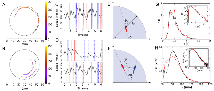
Figure 1: Trajectories along with the bursts (circles) of a fish swimming alone (A) and a group of 2 fish (B). The color of trajectories indicates instantaneous speed. The corresponding speed time series are shown in C and D, along with the acceleration/burst phase delimited by red and blue vertical lines. E defines the variables $r_{\rm w}$ and $\theta_{\rm w}$ (distance and relative orientation to the wall) in order to describe the fish interaction with the wall. F defines the relevant variables $d$, $\psi$, and $\Delta\phi$ (distance, viewing angle, relative orientation of the focal fish with respect to the other fish) in order to describe the influence of the blue fish on the red one. G and H show respectively the probability distribution function (PDF) of the duration and distance traveled between two kicks as measured in the one (black) and two (red) fish experiments (tank of radius $R=250\,$mm). Insets show the corresponding graphs in semi-log scale.

On the other hand, only a few models have been developed to connect a detailed quantitative description of individual-level interactions with the emergent dynamics observed at a group level Herbert2011 ; Gautrais2012 ; Mwaffo2014 . The main difficulty to build such models comes from the entanglement of interactions between an individual and its physical and social environment. To overcome this problem, Gautrais et al. Gautrais2012 have introduced an incremental approach that consists in first building from the experiments a model for the spontaneous motion of an isolated fish Gautrais2009 . This model is then used as a dynamical framework to include the effects of interactions of that fish with the physical environment and with a neighboring fish. The validation of the model is then based on the agreement of its predictions with experiments on several observables in different conditions and group sizes.

In the present work, we use but improve and extend this approach to investigate the swimming behavior and interactions in the red nose fish Hemigrammus rhodostomus. This species performs a burst-and-coast type of swimming that makes it possible to analyze a trajectory as a series of discrete behavioral decisions in time and space. This discreteness of trajectories is exploited to characterize the spontaneous motion of a fish, to identify the candidate stimuli (e.g. the distance, the orientation and velocity of a neighboring fish, or the distance and orientation of the tank wall), and to measure their effects on the behavioral response of a fish. We assume rather general forms for the expected repulsive effect of the tank wall and for the repulsive/attractive and alignment interactions between two fish. These forms take into account the fish anisotropic perception of its physical and social environment and must satisfy some specific symmetry constraints which help us to differentiate these interactions and disentangle their relative contributions. The amount and precision of data accumulated in this work and this modeling approach allow us to reconstruct the actual functional form of the response functions of fish governing their heading changes as a function of the distance, orientation, and angular position relative to an obstacle or a neighbor. We show that the implementation of these interactions in a stochastic model of spontaneous burst-and-glide swimming quantitatively reproduces the motion and spatial distributions observed in experiments with a single fish and with two fish.

II Results

II.1 Characterization of individual swimming behavior

Hemigrammus rhodostomus fish have been monitored swimming alone and freely in shallow water in three different circular tanks of radius $R=176$, 250, 353 mm (see Supplementary Information (SI) for details). This species performs a burst-and-coast type of swimming characterized by sequences of sudden increase in speed followed by a mostly passive gliding period (see SI Movie S1). This allows the analysis of a trajectory as a series of discrete decisions in time. One can then identify the candidate stimuli (e.g. the distance, the orientation and velocity of a neighboring fish, or the distance and orientation of an obstacle) that have elicited a fish response and reconstruct the associated stimulus-response function. Most changes in fish heading occur exactly at the onset of the acceleration phase. We label each of these increases as a “kick”.

Figs. 1A and 1B show typical trajectories of H. rhodostomus swimming alone or in groups of two fish. After the data treatment (see SI and Fig. S1 and S2 there), it is possible to identify each kick (delimited by vertical lines in Figs. 1C and 1D), which we use to describe fish trajectories as a group of straight lines between each of these events. While the average duration between kicks is close to 0.5 s for experiments with one or two fish (Fig. 1G), the mean length covered between two successive kicks is slightly lower for two fish (Fig. 1H). The typical velocity of the fish in their active periods (see SI) is of order 140 mm/s.

II.2 Quantifying the effect of the interaction of a single fish with the wall

Fig. 2A shows the experimental probability density function (PDF) of the distance to the wall $r_{\rm w}$ after each kick, illustrating that the fish spends most of the time very close to the wall. We will see that the combination of the burst-and-coast nature of the trajectories (segments of average length $\sim 70$ mm, but smaller when the fish is very close to the wall) and of the narrow distribution of angle changes between kicks (see Fig. 2D) prevent a fish from efficiently escaping the curved wall of the tank (see SI Movie S2). Fig. 2C shows the PDF of the relative angle of the fish to the wall $\theta_{\rm w}$, centered near, but clearly below 90^∘, as the fish remains almost parallel to the wall and most often goes toward it.

In order to characterize the behavior with respect to the walls, we define the signed angle variation $\delta\phi_{+}=\delta\phi{\times}{\rm Sign}(\theta_{\rm w})$ after each kick, where $\delta\phi$ is the measured angle variation. $\delta\phi_{+}$ is hence positive when the fish goes away from the wall and negative when the fish is heading towards it. The PDF of $\delta\phi_{+}$ is wider than a Gaussian and is clearly centered at a positive $\delta\phi_{+}\approx 15^{\circ}$ (tank of radius $R=353\,$mm), illustrating that the fish works at avoiding the wall (Fig. 2D). When one restricts the data to instances where the fish is at a distance $r_{\rm w}>60\,$mm from the wall, for which its influence becomes negligible (see Fig. 4A and the discussion hereafter), the PDF of $\delta\phi_{+}$ indeed becomes symmetric, independent of the tank in which the fish swims, and takes a quasi Gaussian form of width of order 20^∘ (inset of Fig. 2D). The various quantities displayed in Fig. 2 will ultimately be used to calibrate and test the predictions of our model.

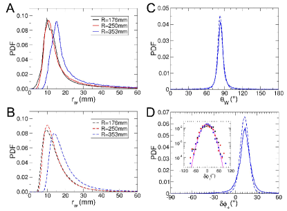
Figure 2: Quantification of the spatial distribution and motion of a fish swimming alone. Experimental (A; full lines) and theoretical (B; dashed lines) PDF of the distance to the wall $r_{\rm w}$ after a kick in the three arenas of radius $R=176$, 250, 353 mm. C: experimental (full line) and theoretical (dashed line) PDF of the relative angle of the fish with the wall $\theta_{\rm w}$ ($R=353\,$mm). D: PDF of the signed angle variation $\delta\phi_{+}=\delta\phi{\times}{\rm Sign}(\theta_{\rm w})$ after each kick ($R=353\,$mm). The inset shows the distribution of $\delta\phi_{+}$ when the fish is near the center of the tank $(r_{\rm w}>60\,$mm), for $R=176$, 250, 353 mm (colored dots), which becomes centered at $\delta\phi_{+}=0^{\circ}$ and Gaussian of width $\approx 20^{\circ}$ (full line).

II.3 Modeling and direct measurement of fish interaction with the wall

We first define a simple model for the spontaneous burst-and-coast motion of a single fish without any wall boundaries, and then introduce the fish-wall interaction, before considering the interaction between two fish in the next subsection D. The large amount of data accumulated (more than 300000 recorded kicks for 1 fish, and 200000 for 2 fish; see SI) permits us to not only precisely characterize the interactions, but also to test the model by comparing its results to various experimental quantities which would be very sensitive to a change in model and/or parameters (e.g. the full fish-wall and fish-fish distance and angle distributions instead of simply their mean).

II.3.1 Swimming dynamics without any interaction

We model the burst-and-coast motion by a series of instantaneous kicks each followed by a gliding period where fish travel in straight lines with a decaying velocity. At the $n$-th kick, the fish located at $\vec{x}_{n}$ at time $t_{n}$ with angular direction $\phi_{n}$ randomly selects a new heading angle $\phi_{n+1}$, a start or peak speed $v_{n}$, a kick duration $\tau_{n}$, and a kick length $l_{n}$. During the gliding phase, the speed is empirically found to decrease quasi exponentially to a good approximation, as shown on Fig. 3, with a decay or dissipation time $\tau_{0}\approx 0.80\,$s, so that knowing $v_{n}$ and $\tau_{n}$ or $v_{n}$ and $l_{n}$, the third quantity is given by $l_{n}=v_{n}\tau_{0}(1-\exp[-\frac{\tau_{n}}{\tau_{0}}])$. At the end of the kick, the position and time are updated to

$$\vec{x}_{n+1}=\vec{x}_{n}+l_{n}\vec{e}(\phi_{n+1}),\quad t_{n+1}=t_{n}+\tau_{n},$$ (1)

where $\vec{e}(\phi_{n+1})$ is the unit vector along the new angular direction $\phi_{n+1}$ of the fish. In practice, we generate $v_{n}$ and $l_{n}$, and hence $\tau_{n}$ from simple model bell-shaped probability density functions (PDF) consistent with the experimental ones shown in Figs. 1G and 1H. In addition, the distribution of $\delta\phi_{\rm R}=\phi_{n+1}-\phi_{n}$ (the ${\rm R}$ subscript stands for “random”) is experimentally found to be very close to a Gaussian distribution when the fish is located close to the center of the tank, $i.e.$ when the interaction with the wall is negligible (see the inset of Fig. 2D). $\delta\phi_{\rm R}$ describes the spontaneous decisions of the fish to change its heading:

$$\phi_{n+1}=\phi_{n}+\delta\phi_{\rm R}=\phi_{n}+\gamma_{\rm R}\,g,$$ (2)

where $g$ is a Gaussian random variable with zero average and unit variance, and $\gamma_{\rm R}$ is the intensity of the heading direction fluctuation, which is found to be of order 0.35 radian ($\approx 20^{\circ}$) in the three tanks.

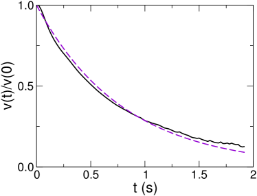
Figure 3: Average decay of the fish speed right after a kick (black line), which can be reasonably described by an exponential decay with a relaxation time $\tau_{0}\approx 0.80\,$s (violet dashed line)

By exploiting the burst-and-coast dynamics of H. rhodostomus, we have defined an effective kick dynamics, of length and duration $l_{n}$ and $\tau_{n}$. However, it can be useful to generate the full continuous time dynamics from this discrete dynamics. For instance, such a procedure is necessary to produce “real-time” movies of fish trajectories obtained from the model (see SI Movies S2, S4, and S5). As already mentioned, during a kick, the speed is empirically found to decrease exponentially to a good approximation (see Fig. 3), with a decay or dissipation time $\tau_{0}\approx 0.80\,$s. Between the time $t_{n}$ and $t_{n+1}=t_{n}+\tau_{n}$, the viscous dynamics due to the water drag for $0\leq t\leq\tau_{n}$ leads to

$$\vec{x}(t_{n}+t)=\vec{x}_{n}+l_{n}\frac{1-\exp[-\frac{t}{\tau_{0}}]}{1-\exp[-\frac{\tau_{n}}{\tau_{0}}]}\vec{e}(\phi_{n+1}),$$ (3)

so that one recovers $\vec{x}(t_{n}+\tau_{n})=\vec{x}(t_{n+1})=\vec{x}_{n}+l_{n}\vec{e}(\phi_{n+1})=\vec{x}_{n+1}$.

II.3.2 Fish interaction with the wall

In order to include the interaction of the fish with the wall, we introduce an extra contribution $\delta\phi_{\rm W}$

$$\delta\phi=\delta\phi_{\rm R}(r_{\rm w})+\delta\phi_{\rm W}(r_{\rm w},\theta_{\rm w}),$$ (4)

where, due to symmetry constraints in a circular tank, $\delta\phi_{\rm W}$ can only depend on the distance to the wall $r_{\rm w}$, and on the angle $\theta_{\rm w}$ between the fish angular direction $\phi$ and the normal to the wall (pointing from the tank center to the wall; see Fig. 1E). We did not observe any statistically relevant left/right asymmetry, which imposes the symmetry condition

$$\delta\phi_{\rm W}(r_{\rm w},-\theta_{\rm w})=-\delta\phi_{\rm W}(r_{\rm w},\theta_{\rm w}).$$ (5)

The random fluctuations of the fish direction are expected to be reduced when it stands near the wall, as the fish has less room for large angles variations (compare the main plot and the inset of Fig. 2D), and we now define

$$\delta\phi_{\rm R}(r_{\rm w})=\gamma_{\rm R}[1-\alpha f_{\rm w}(r_{\rm w})]g.$$ (6)

$f_{\rm w}(r_{\rm w})\to 0$, when $r_{\rm w}\gg l_{\rm w}$ (where $l_{\rm w}$ sets the range of the wall interaction), recovering the free spontaneous motion in this limit. In addition, we define $f_{\rm w}(0)=1$ so that the fluctuations near the wall are reduced by a factor $1-\alpha$, which is found experimentally to be close to $1/3$, so that $\alpha\approx 2/3$.

If the effective “repulsive force” exerted by the wall on the fish (first considered as a physical particle) tends to make it go toward the center of the tank, it must take the form $\delta\phi_{\rm W}(r_{\rm w},\theta_{\rm w})=\gamma_{\rm W}\sin(\theta_{\rm w})f_{\rm w}(r_{\rm w})$, where the term $\sin(\theta_{\rm w})$ is simply the projection of the normal to the wall (i.e. the direction of the repulsion “force” due to the wall) on the angular acceleration of the fish (of direction $\phi+90^{\circ})$. For the sake of simplicity, $f_{\rm w}(r_{\rm w})$ is taken as the same function as the one introduced in Eq. (6), as it satisfies the same limit behaviors. In fact, a fish does not have an isotropic perception of its environment. In order to take into account this important effect in a phenomenological way, we introduce $\epsilon_{\rm w}(\theta_{\rm w})=\epsilon_{w,1}\cos(\theta_{\rm w})+\epsilon_{w,2}\cos(2\theta_{\rm w})+...$, an even function (by symmetry) of $\theta_{\rm w}$, which, we assume, does not depend on $r_{\rm w}$, and finally define

$$\delta\phi_{\rm W}(r_{\rm w},\theta_{\rm w})=\gamma_{\rm W}\sin(\theta_{\rm w})[1+\epsilon_{\rm w}(\theta_{\rm w})]f_{\rm w}(r_{\rm w}),$$ (7)

where $\gamma_{\rm W}$ is the intensity of the wall repulsion.

Once the displacement $l$ and the total angle change $\delta\phi$ have been generated as explained above, we have to eliminate the instances where the new position of the fish would be outside the tank. More precisely, and since $\vec{x}$ refers to the position of the center of mass of the fish (and not of its head) before the kick, we introduce a “comfort length” $l_{c}$, which must be of the order of one body length (BL; 1 BL$\,\sim 30\,$mm; see SI), and we reject the move if the point $\vec{x}+(l+l_{c})\vec{e}(\phi+\delta\phi)$ is outside the tank. When this happens, we regenerate $l$ and $\delta\phi$ (and in particular, its random contribution $\delta\phi_{\rm R}$), until the new fish position is inside the tank. Note that in the rare cases where such a valid couple is not found after a large number of iterations (say, 1000), we generate a new value of $\delta\phi_{\rm R}$ uniformly drawn in $[-\pi,\pi]$ until a valid solution is obtained. Such a large angle is for instance necessary (and observed experimentally), when the fish happens to approach the wall almost perpendicularly to it ($\delta\phi\sim 90^{\circ}$ or more; see Movie S5 at 20 s, where the red fish performs such a large angle change).

In order to measure experimentally $\epsilon_{\rm w}(\theta_{\rm w})$ and $f_{\rm w}(r_{\rm w})$, and confirm the functional form of Eq. (7), we define a fitting procedure which is explicitly described in SI, by minimizing the error between the experimental $\delta\phi$ and a general product functional form $\delta\phi_{\rm W}(r_{\rm w},\theta_{\rm w})=f_{\rm w}(r_{\rm w})O_{\rm w}(\theta_{\rm w})$, where the only constraint is that $O_{\rm w}(\theta_{\rm w})$ is an odd function of $\theta_{\rm w}$ (hence the name $O$), in order to satisfy the symmetry condition of Eq. (5). Since multiplying $O_{\rm w}$ by an arbitrary constant and dividing $f_{\rm w}$ by the same constant leaves the product unchanged, we normalize $O_{\rm w}$ (and all angular functions appearing below) such that its average square is unity: $\frac{1}{2\pi}\int_{-\pi}^{+\pi}O_{\rm w}^{2}(\theta_{\rm w})\,d\theta_{\rm w}=1$.

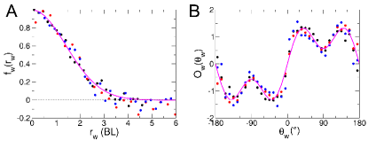
Figure 4: Interaction of a fish with the tank wall as a function of its distance $r_{\rm w}$ (A) and its relative orientation to the wall $\theta_{\rm w}$(B) as measured experimentally in the three tanks of radius $R=176\,$mm (black), $R=250\,$mm (blue), $R=353\,$mm (red). The full lines correspond to the analytic forms of $f_{\rm w}(r_{\rm w})$ and $O_{\rm w}(\theta_{\rm w})$ given in the text. In particular, $f_{\rm w}(r_{\rm w})$ is well approximated by a Gaussian of width $l_{\rm w}\approx 2\,$BL$\sim 60\,$mm.

For each of the three tanks, the result of this procedure is presented as a scatter plot in Figs. 4A and 4B respectively, along with the simple following functional forms (solid lines)

$$O_{\rm w}(\theta_{\rm w})\propto\sin(\theta_{\rm w})[1+0.7\cos(2\theta_{\rm w})],$$ (8)

$$f_{\rm w}(r_{\rm w})=\exp\left[-\left(r_{\rm w}/l_{\rm w}\right)^{2}\right],~{}{\rm with}~{}l_{\rm w}\approx 2\,{\rm BL}.$$ (9)

Hence, we find that the range of the wall interaction is of order $l_{\rm w}\approx 2\,{\rm BL}\sim 60\,$mm, and is strongly reduced when the fish is parallel to the wall (corresponding to a “comfort” situation), illustrated by the deep (i.e. lower response) observed for $\theta_{\rm w}\approx 90^{\circ}$ in Fig. 4B ($\cos(2\theta_{\rm w})\approx-1$). Moreover, we do not find any significative dependence of these functional forms with the radius of the tank, although the interaction strength $\gamma_{W}$ is found to decrease as the radius of the wall increases (see Table S3). The smaller is the tank radius (of curvature), the more effort is needed by the fish to avoid the wall.

Note that the fitting procedure used to produce the results of Fig. 4 (described in detail in the SI) does not involve any regularization scheme imposing the scatter plots to fall on actual continuous curves. The fact that they actually do describe such fairly smooth curves (as we will also find for the interaction functions between two fish; see Fig. 6) is an implicit validation of our procedure.

In Fig. 2, and for the three tank radii considered, we compare the distribution of distance to the wall $r_{w}$, relative angle to the wall $\theta_{w}$, and angle change $\delta\phi$ after each kick, as obtained experimentally and in extensive numerical simulations of the model, finding an overall satisfactory agreement. On a more qualitative note, the model fish dynamics mimics fairly well the behavior and motion of a real fish (see SI Movie S2).

II.4 Quantifying the effect of interactions between two fish

Experiments with two fish were performed using the tank of radius $R=250\,$mm; and a total of around 200000 kicks were recorded (see SI for details).

In Fig. 5, we present various experimental PDF which characterize the swimming behavior of two fish resulting from their interaction, and which will permit to calibrate and test our model. Fig. 5A shows the PDF of the distance to the wall, for the geometrical “leader” and “follower” fish. The geometrical leader is defined as the fish with the largest viewing angle $|\psi|\in[0,180^{\circ}]$ (see Fig. 1F where the leader is the red fish), that is, the fish which needs to turn the most to directly face the other fish. Note that the geometrical leader is not always the same fish, as they can exchange role (see SI Movie S5). We find that the geometrical leader is much closer to the wall than the follower, as the follower tries to catch up and hence hugs the bend. Still, both fish are farther from the wall than an isolated fish is (see Fig. 2A; also compare SI Movie S2 and S4). The inset of Fig. 5A shows the PDF of the distance $d$ between the two fish, illustrating the strong attractive interaction between them.

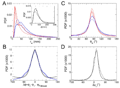
Figure 5: Quantification of the spatial distribution and motion in groups of two fish. In all graphs, full lines correspond to experimental results and dashed lines to numerical simulations of the model. A: PDF of the distance to the wall, for the geometrical leader (red) and follower (blue) fish; the inset displays the PDF of the distance $d$ between the two fish. B: PDF of the relative orientation $\Delta\phi=\phi_{2}-\phi_{1}$ between the two fish (black) and PDF of the viewing angle $\psi$ of the follower (blue). C: PDF of the relative angle to the wall $\theta_{\rm w}$ for the leader (red) and follower fish (blue). D: PDF (averaged over both fish) of the signed angle variation $\delta\phi_{+}=\delta\phi{\times}{\rm Sign}(\theta_{\rm w})$ after each kick.

Fig. 5C shows the PDF of $\theta_{\rm w}$ for the leader and follower fish, which are again much wider than for an isolated fish (see Fig. 2C). The leader being closer and hence more parallel to the wall displays a sharper distribution than the follower. Fig. 5B shows the PDF of the relative orientation $\Delta\phi=\phi_{2}-\phi_{1}$ between the two fish, illustrating their tendency to align, along with the PDF of the viewing angle $\psi$ of the follower. Both PDF are found to be very similar and peaked at 0^∘. Finally, Fig. 5D shows the PDF (averaged over both fish) of the signed angle variation $\delta\phi_{+}=\delta\phi{\times}{\rm Sign}(\theta_{\rm w})$ after each kick, which is again much wider than for an isolated fish (Fig. 2D). Due to their mutual influence, the fish swim farther from the wall than an isolated fish, and the wall constrains less their angular fluctuations.

II.5 Modeling and direct measurement of interactions between two fish

In the presence of an other fish, the total heading angle change now reads

$$\delta\phi = \delta\phi_{\rm R}(r_{\rm w})+\delta\phi_{\rm W}(r_{\rm w},\theta_{\rm w})+$$

$$\delta\phi_{\rm Att}(d,\psi,\Delta\phi)+\delta\phi_{\rm Ali}(d,\psi,\Delta\phi),$$

where the random and wall contributions are given by Eqs. (6,7,8,9), and the two new contributions results from the expected attraction and alignment interactions between fish. The distance between fish $d$, the relative position or viewing angle $\psi$, and the relative orientation angle $\Delta\phi$ are all defined in Fig. 1F. By mirror symmetry already discussed in the context of the interaction with the wall, one has the exact constraint

$$\delta\phi_{\rm Att,\,Ali}(d,-\psi,-\Delta\phi)=-\delta\phi_{\rm Att,\,Ali}(d,\psi,\Delta\phi),$$ (11)

meaning that a trajectory of the two fish observed from above the tank has the same probability of occurrence as the same trajectory as it appears when viewing it from the bottom of the tank. We hence propose the following product expressions

$$\delta\phi_{\rm Att}(d,\psi,\Delta\phi)=F_{\rm Att}(d)O_{\rm Att}(\psi)E_{\rm Att}(\Delta\phi),$$ (12)

$$\delta\phi_{\rm Ali}(d,\psi,\Delta\phi)=F_{\rm Ali}(d)O_{\rm Ali}(\Delta\phi)E_{\rm Ali}(\psi),$$ (13)

where the functions $O$ are odd, and the functions $E$ are even. For instance, $O_{\rm Att}$ must be odd as the focal fish should turn by the same angle (but of opposite sign) whether the other fish is at the same angle $|\psi|$ to its left or right. Like in the case of the wall interaction, we normalize the four angular functions appearing in Eqs. (12,13) such that their average square is unity. Both attraction and alignment interactions clearly break the law of action and reaction, as briefly mentioned in the Introduction and discussed in the Appendix. Although the heading angle difference perceived by the other fish is simply $\Delta\phi^{\prime}=-\Delta\phi$, its viewing angle $\psi^{\prime}$ is in general not equal to $-\psi$ (see Fig. 1F).

As already discussed in the context of the wall interaction, an isotropic radial attraction force between the two fish independent of the relative orientation, would lead exactly to Eq. (12), with $O_{\rm Att}(\psi)\sim\sin(\psi)$ and $E_{\rm Att}(\Delta\phi)=1$. Moreover, an alignment force tending to maximize the scalar product, $i.e.$ the alignment, between the two fish headings takes the natural form $O_{\rm Ali}(\Delta\phi)\sim\sin(\Delta\phi)$, similar to the one between two magnetic spins, for which one has $E_{\rm Ali}(\psi)=1$. However, we allow here for more general forms satisfying the required parity properties, due to the fish anisotropic perception of its environment, and to the fact that its behavior may also be affected by its relative orientation with the other fish. For instance, we anticipate that $E_{\rm Ali}(\psi)$ should be smaller when the other fish is behind the focal fish ($\psi=180^{\circ}$; bad perception of the other fish direction) than when it is ahead ($\psi=0^{\circ}$).

As for the dependence of $F_{\rm Att}$ with the distance between fish $d$, we expect $F_{\rm Att}$ to be negative (repulsive interaction) at short distance $d\leq d_{0}\sim 1\,$BL, and then to grow up to a typical distance $l_{\rm Att}$, before ultimately decaying above $l_{\rm Att}$. Note that if the attraction force is mostly mediated by vision at large distance, it should be proportional to the 2D solid angle produced by the other fish, which decays like $1/d$, for large $d$. These considerations motivate us to introduce an explicit functional form satisfying all these requirements

$$F_{\rm Att}(d)\propto\frac{d-d_{0}}{1+(d/l_{\rm Att})^{2}}.$$ (14)

$F_{\rm Ali}$ should be dominant at short distance, before decaying for $d$ greater than some $l_{\rm Ali}$ defining the range of the alignment interaction. For large distance $d$, the alignment interaction should be smaller than the attraction force, as it becomes more difficult for the focal fish to estimate the precise relative orientation of the other fish than to simply identify its presence.

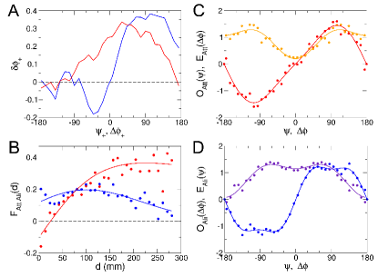
Figure 6: Quantification and modeling of interactions between pairs of fish. A: we plot the average signed angle change after a kick $\delta\phi_{+}=\delta\phi{\times}{\rm Sign}(\psi)$ $vs$ $\Delta\phi{\times}{\rm Sign}(\psi)$ (red) and $\delta\phi_{+}=\delta\phi{\times}{\rm Sign}(\Delta\phi)$ $vs$ $\psi{\times}{\rm Sign}(\Delta\phi)$ (blue) (see text). B: dependence of the attraction ($F_{\rm Att}(d)$ in red) and alignment ($F_{\rm Ali}(d)$ in blue) interactions with the distance $d$ between fish. The full lines correspond to the physically motivated form of Eq. (14) (red), and the fit proposed in the text for $F_{\rm Ali}(d)$ (blue). C: $O_{\rm Att}(\psi)$ (odd function in red) and $E_{\rm Att}(\Delta\phi)$ (even function in orange) characterize the angular dependence of the attraction interaction, and are defined in Eq. (12). D: $O_{\rm Ali}(\Delta\phi)$ (odd function in blue) and $E_{\rm Ali}(\psi)$ (even function in violet), defined in Eq. (13), characterize the angular dependence of the alignment interaction. Dots in B, C, and D correspond to the results of applying the procedure explained in SI to extract the interaction functions from experimental data.

Fig. 6A shows strong evidence for the existence of an alignment interaction. Indeed, we plot the average signed angle change after a kick $\delta\phi_{+}=\delta\phi{\times}{\rm Sign}(\psi)$ $vs$ $\Delta\phi{\times}{\rm Sign}(\psi)$ and $\delta\phi_{+}=\delta\phi{\times}{\rm Sign}(\Delta\phi)$ $vs$ $\psi{\times}{\rm Sign}(\Delta\phi)$. In accordance with Eqs. (12,13), a strong positive $\delta\phi_{+}$ when the corresponding variable is positive indicates that the fish changes more its heading if it favors mutual alignment (reducing $\Delta\phi$), for the same viewing angle $\psi$.

As precisely explained in SI, we have determined the six functions appearing in Eqs. (12,13) by minimizing the error with the measured $\delta\phi$, only considering kicks for which the focal fish was at a distance $r_{\rm w}>2\,$BL from the wall, in order to eliminate its effect (see Fig. 4A). This procedure leads to smooth and well behaved measured functions displayed in Fig. 6. As shown in Fig. 6B, the functional form of Eq. (14) adequately describes $F_{\rm Att}(d)$, with $l_{\rm Att}\approx 200\,$mm, and with an apparent repulsive regime at very short range, with $d_{0}\approx 30\,{\rm mm}\sim 1\,$BL. The crossover between a dominant alignment interaction to a dominant attraction interaction is also clear. The blue full line in Fig. 6B, a guide to the eye reproducing appropriately $F_{\rm Ali}(d)$, corresponds to the phenomenological functional form

$$F_{\rm Ali}(d)\propto(d+d_{0}^{\prime})\exp[-(d/l_{\rm Ali})^{2}],$$ (15)

with $l_{\rm Ali}\approx 200\,$mm. Note that $F_{\rm Att}(d)$ and $F_{\rm Ali}(d)$ cannot be properly measured for $d>280$ mm due to the lack of statistics, the two fish remaining most of the time close to each other (see the inset of Fig. 6A; the typical distance between fish is $d\sim 75\,$mm).

Fig. 6C shows $O_{\rm Att}(\psi)\propto\sin(\psi)[1+\epsilon_{\rm Att,1}\cos(\psi)+...]$ (odd function) and $E_{\rm Att}(\Delta\phi)\propto 1+\eta_{\rm Att,1}\cos(\Delta\phi)+...$ (even function) along with fits involving no more than 2 non zero Fourier coefficients (and often only one; see SI for their actual values). $E_{\rm Att}(\Delta\phi)$ has a minimum for $\Delta\phi=0$ indicating that the attraction interaction is reduced when both fish are aligned. Similarly, Fig. 6D shows $O_{\rm Ali}(\Delta\phi)$ and $E_{\rm Ali}(\psi)$ and the corresponding fits. As anticipated, the alignment interaction is stronger when the influencing fish is ahead of the focal fish ($|\psi|<90^{\circ}$), and almost vanishes when it is behind ($\psi=\pm 180^{\circ}$).

In Fig. 5, we compare the results of extensive numerical simulations of the model including the interactions between fish to experimental data, finding an overall qualitative (SI Movie S4 and SI Movie S5) and quantitative agreement.

As a conclusion of this section, we would like to discuss the generality of the product functional forms of Eqs. (12,13) for the interaction between fish, or of Eq. (7) in the context of the wall interaction. As already briefly mentioned, for a physical point particle interacting through a physical force like gravity, the angle change $\delta\phi_{\rm Att}(d,\psi)$ would be the projection of the radial force onto the angular acceleration (normal to the velocity of angular direction $\psi$ relative to the vector between the two particles) and would then exactly take the form $F_{\rm Att}(d){\times}\sin(\psi)$. Hence, Eq. (12) (resp. Eq. (7), for the wall interaction) is the simplest generalization accounting for the fish anisotropic perception of its environment, while keeping a product form and still obeying the left/right symmetry condition of Eq. (11) (resp. of Eq. (5)). In principle, $\delta\phi_{\rm Att}(d,\psi,\Delta\phi)$ should be written most generally as an expansion $\sum_{i}F_{{\rm Att},i}(d)O_{{\rm Att},i}(\psi)E_{{\rm Att},i}(\Delta\phi)$. However, as the number of terms of this expansion increases, we run the risk of overfitting the experimental data by the procedure detailed in the SI. In addition, the leading term of this expansion would still capture the main behavioral effects of the interaction and should be very similar to the results of Fig. 6, while the weaker remaining terms would anyway be difficult to interpret. Note that the same argument applies to the alignment interaction, when exploiting the analogy with the magnetic alignment force between two spins. Eq. (13) is the simplest generalization of the interaction $\delta\phi_{\rm Ali}(d,\Delta\phi)=F_{\rm Ali}(d)\sin(\Delta\phi)$ obtained in this case, while preserving the left/righ symmetry and product form. Considering the fact that no regularization or smoothing procedure was used in our data analysis (see SI), the quality (low noise, especially for angular functions) of the results presented in Figs. 4 and 6 strongly suggests that the generalized product forms used here capture most of the features of the actual experimental angle change.

III Discussion and conclusion

Characterizing the social interactions between individuals as well as their behavioral reactions to the physical environment is a crucial step in our understanding of complex collective dynamics observed in many group living species and their impact on individual fitness Camazine2001 ; Krause2002 . In the present work, we have analyzed the behavioral responses of a fish to the presence in its neighborhood of an obstacle and to a conspecific fish. In particular, we used the discrete decisions (kicks) of H. rhodostomus to control its heading during burst-and-coast swimming as a proxy to measure and model individual-level interactions. The large amount of data accumulated allowed us to disentangle and quantify the effects of these interactions on fish behavior with a high level of accuracy.

We have quantified the spontaneous swimming behavior of a fish and modeled it by a kick dynamics with Gaussian distributed angle changes. We found that the interactions of fish with an obstacle and a neighboring fish result from the combination of four behavioral modes:

(1) wall avoidance, whose effect starts to be effective when the fish is less than 2 BL from a wall;

(2) short-range repulsion between fish, when inter-individual distance is less than 30 mm ($\sim 1$ BL);

(3) attraction to the neighboring fish, which reaches a maximum value around 200 mm ($\sim 6$ to 7 BL) in our experimental conditions;

(4) alignment to the neighbor, which saturates around 100 mm ($\sim 3$ BL).

In contrast to previous phenomenological models, these behavioral modes are not fixed to discrete and somewhat arbitrary zones of distances in which the neighboring fish are found Aoki1982 ; Huth1992 ; couzin2002 . Instead, there is a continuous combination of attraction and alignment as a function of the distance between fish. Alignment dominates attraction up to $\sim 75$ mm ($\sim 2.5$ BL) while attraction becomes dominant for larger distances. As distance increases even more, attraction must decrease as well. However, the limited size of the experimental tanks and the lack of sufficient data for large $d$ prevented us from measuring this effect, suggesting the long-range nature of the attraction interaction mediated by vision. Note that a cluster of fish can elicit a higher level of attraction, proportional to the 3D solid angle of the fish group as seen by the focal fish, as suggested by models based on visual perception Pita2015 ; Collignon2016 , and as captured by the power-law decay proposed in Eq. (14). Designing experiments to test and quantify the long-range nature of the attraction interaction between fish would be of clear interest.

Moreover, the behavioral responses are strongly modulated by the anisotropic perception of fish. The wall repulsion effect is maximum when the orientation of the fish with regards to the wall is close to 45^∘ and minimum when the fish is parallel to the wall. Likewise, the maximum amplitude alignment occurs when a neighboring fish is located on the front left or right and vanishes as its position around the focal fish moves towards the back.

To quantify separately the effects of attraction and alignment, we exploited physical analogies and symmetry considerations to extract the interactions between a focal fish and the wall and with another fish. Previous studies have shown that in the Golden shiners Katz2011 and the Mosquito fish Herbert2011 , there was no clear evidence for an explicit matching of body orientation. In these species, the alignment between fish was supposed to results from a combination of attraction and repulsion. However, at least in the Mosquito fish, it is likely that the strength of alignment could have been underestimated because the symmetry constraints on alignment and attraction were not taken into consideration. In the Rummy-nose tetra, we find strong evidence for the existence of an explicit alignment.

The characterization and the measurement of burst-and-coast swimming and individual interactions were then used to build and calibrate a model that quantitatively reproduces the dynamics of swimming of fish alone and in groups of two and the consequences of interactions on their spatial and angular distributions. The model shows that the wall avoidance behavior coupled with the burst-and-coast motion results in an unexpected concentration of fish trajectories close to the wall, as observed in our experiments. In fact, this phenomenon is well referenced experimentally for run-and-tumble swimming (for instance, in sperm cells RTexp1 or bacteria RTexp2 ). It can be explained theoretically and reproduced in simple models RTth1 ; RTth2 , as the effective discreteness of the trajectories separated in bursts or tumbles prevents the individuals from escaping the wall. Our model also reproduces the alternation of temporary leaders and followers in groups of two fish, the behavior of the temporary leader being mostly governed by its interactions with the wall, while the temporary follower is mostly influenced by the behavior of the temporary leader.

This validated model can serve as a basis for testing hypotheses on the combination of influence exerted by multiples neighbors on a focal fish in tanks of arbitrary shape. Moreover, it would certainly be interesting to study theoretically the dynamics of many fish swimming without any boundary and according to the found interactions. The study of the phase diagram as a function of the strength of the attraction and alignment interactions (and possibly their range) should show the emergence of various collective phases (schooling phase, vortex phase…) Tunstrom2013 ; Calovi2014 .

Finally, our method has proved successful in disentangling and fully characterizing the interactions that govern the behavior of pairs of animals when large amount of data are available. Hence, it could be successfully applied to collective motion phenomena occurring in various biological systems at different scales of organization.

Contribution of authors

C.S. and G.T. designed research; D.S.C., V.L., U.L., and G.T. performed research; D.S.C., A.L., and C.S. developed the model; D.S.C., A.L., V.L., U.L., H.C., C.S., and G.T. analyzed data; A.P.E. contributed new reagents/analytic tools; V.L., C.S., and G.T. wrote the paper.

Appendix A Intelligent and dumb active matter

A rather general equation describing the dynamics of a standard physical particle moving in a thermal bath (or a medium inducing a friction and a random stochastic force, like a gas) and submitted to physical external forces $\vec{F}_{\rm Phys}(\vec{x})$ (due to other particles and/or external fields) reads

$$\frac{d\vec{v}}{dt}=-\frac{\vec{v}}{\tau}+\vec{F}_{\rm Phys}+\sqrt{\frac{2T}{\tau}}\vec{\eta},$$ (16)

where $\vec{v}=\frac{d\vec{x}}{dt}$ is the particle velocity, $T$ is the temperature, and $\vec{\eta}(t)$ is a stochastic Gaussian noise, delta-correlated in time, $\langle\vec{\eta}(t)\vec{\eta}(t^{\prime})\rangle=\delta(t-t^{\prime})$. In particular, if the physical force is conservative and hence is the gradient of a potential $V_{\rm Phys}(\vec{x})$, the stationary velocity and position probability distribution of the particle produced by this equation is well known to be the Boltzmann distribution,

$$P(\vec{x},\vec{v})=\frac{1}{Z}{\exp\left(-\frac{E}{T}\right)},$$ (17)

where $E=\frac{v^{2}}{2}+V_{\rm Phys}$ is the energy, and $Z$ is a normalization constant.

A.1 Dumb active matter

An active particle is characterized by its intrinsic or desired velocity $\vec{u}$. Its actual velocity $\vec{v}=\frac{d\vec{x}}{dt}$ rather generally obeys an equation similar to Eq. (16):

$$\frac{d\vec{v}}{dt}=-\frac{\vec{v}-\vec{u}}{\tau}+\vec{F}_{\rm Phys}+\sqrt{\frac{2T}{\tau}}\vec{\eta},$$ (18)

where the first term on the right hand side tends to make the actual velocity go to the intrinsic velocity. Eq. (18) has to be supplemented with a specific equation for the intrinsic velocity. Here, for the sake of simplicity, we assume that $\vec{u}$ is a simple Ornstein-Uhlenbeck stochastic process,

$$\frac{d\vec{u}}{dt}=-\frac{\vec{u}}{\tau^{\prime}}+\sqrt{\frac{2T^{\prime}}{\tau}}\vec{\eta^{\prime}},$$ (19)

where $\vec{\eta^{\prime}}$ is an other stochastic Gaussian noise, uncorrelated with $\vec{\eta}$, and $\tau^{\prime}$ is some correlation time, a priori unrelated to $\tau$. In general, the stationary distribution $P(\vec{x},\vec{v},\vec{u})$ is not known, although some analytical results can be obtained in some limits (for instance, large friction, and separation of the time scales $\tau$ and $\tau^{\prime}$) Col1 ; Col2 .

A first limiting case of this equation is the strong friction limit (small $\tau$), where the inertial term in Eq. (18) becomes negligible, leading to

$$\frac{d\vec{x}}{dt}=\vec{v}=\vec{u}+{\tau}\vec{F}_{\rm Phys}+\sqrt{2T\tau}\vec{\eta}.$$ (20)

In the limit of a “cold” medium, where the stochastic force is absent or negligible, we obtain

$$\vec{v}=\vec{u}+{\tau}\vec{F}_{\rm Phys}.$$ (21)

Note that in Eqs. (18,19,20,21), the physical force directly impacts the final velocity $\vec{v}$, but not the intrinsic velocity $\vec{u}$ of the active particle. This very property constitutes our definition of a “dumb” active particle.

A.2 Intelligent active matter

As explained in the Introduction, animals can not only be submitted to physical forces $\vec{F}_{\rm Phys}$ (e.g. a human physically pushing an other one), but mostly react to “social forces” $\vec{F}_{\rm Soc}$. These social interactions directly affect the intrinsic velocity of the active particle, which constitutes our definition of an “intelligent” active particle. In the “cold” limit relevant for fish or humans (the substrate in which they move does not exert any noticeable random force), the system of equations Eqs. (18,19) becomes

$$\frac{d\vec{v}}{dt}=-\frac{\vec{v}-\vec{u}}{\tau}+\vec{F}_{\rm Phys},$$ (22)

$$\frac{d\vec{u}}{dt}=-\frac{\vec{u}}{\tau^{\prime}}+\vec{F}_{\rm Soc}+\sqrt{\frac{2T^{\prime}}{\tau}}\vec{\eta^{\prime}},$$ (23)

In the context of animal and intelligent active matter, the stochastic noise $\vec{\eta^{\prime}}$ modelizes the spontaneous motion – the “free will” – of the animal (see Eq. (2), for Hemigrammus rhodostomus).

Moreover, we also already mentioned that these social forces are in general non conservative and hence strongly break the action-reaction law, as they generally depend not only on the positions of the particles, but also on their velocities (their relative direction $\Delta\phi$ and the viewing angle $\psi$ and $\theta_{\rm w}$ defined in Fig. 1). In the present work, we have for instance showed how the interaction of Hemigrammus rhodostomus with a circular wall depend not only on the distance to the wall, but also on the viewing angle $\theta_{\rm w}$ between the fish heading and the normal to the wall (see Fig. 4). We also determined the dependence of the attraction and alignment interactions on the focal fish viewing angle $\psi$ and the two fish relative heading angle $\Delta\phi$ (see Fig. 6). Note that physical forces can induce a cognitive reaction and hence a change in the intrinsic velocity, so that $\vec{F}_{\rm Soc}$ may also contain reaction term to the presence of physical forces $\vec{F}_{\rm Phys}$ (this was not the case in our experiments, except maybe, when the fish would actually touch the wall). Conversely, social interaction may lead to a particle willingly applying a physical force (a human moving toward an other one and then pushing her/him). As a consequence, the notion of a conserved energy and many other properties resulting from the conservative nature of standard physical forces are lost, leading to a much more difficult analytical analysis of the Fokker-Planck equation which can be derived from Eqs. (22,23).

It is obviously a huge challenge to characterize these social interactions in animal groups, in particular to better understand the collective phenomena emerging in various contexts Camazine2001 ; Giardina2008 ; Sumpter2010 . The system of equations Eqs. (22,23), for specific social interactions, also presents a formidable challenge, for instance to determine the stationary distribution $P(\vec{x},\vec{v},\vec{u})$. In the absence of physical forces, and in the limit of fast reaction (small $\tau$), leading to a perfect matching between the velocity and the intrinsic velocity, we obtain

$$\vec{v}=\frac{d\vec{x}}{dt}=\vec{u},$$ (24)

$$\frac{d\vec{u}}{dt}=-\frac{\vec{u}}{\tau^{\prime}}+\vec{F}_{\rm Soc}+\sqrt{\frac{2T^{\prime}}{\tau}}\vec{\eta^{\prime}}.$$ (25)

Interestingly, this system is formally equivalent to Eq. (16) for a standard physical particle, although Eq. (25) is formally an equation for the intrinsic velocity, equal to the actual velocity in the considered limit. Yet, the resulting stationary state $P(\vec{x},\vec{v}=\vec{u})$ is in general not known, because of the non conservative nature of the social interactions discussed above and in the Introduction.

References

- (1) A. Brown and W. Poon. Ionic effects in self-propelled Pt-coated Janus swimmers. Soft matter 10.22 (2014), 4016–4027.
- (2) A. Walther and A. H. E. Müller. Janus particles. Soft Matter 4.4 (2008), 663.
- (3) J. R. Howse, R. A. Jones, A. J. Ryan, T. Gough, R. Vafabakhsh and R. Golestanian. Self-motile colloidal particles: from directed propulsion to random walk. Phys. Rev. Lett. 99.4 (2007), 048102.
- (4) I. Theurkauff, C. Cottin-Bizonne, J. Palacci, C. Ybert, and L. Bocquet. Dynamic clustering in active colloidal suspensions with chemical signaling. Phys. Rev. Lett. 108.26 (2012), 268303.
- (5) J. Palacci, C. Cottin-Bizonne, C. Ybert, and L. Bocquet. Sedimentation and effective temperature of active colloidal suspensions. Phys. Rev. Lett. 105.8 (2010), 088304.
- (6) J. Palacci, S. Sacanna, A. P. Steinberg, D. J. Pine, and P. M. Chaikin. Living crystals of light-activated colloidal surfers. Science 339.6122 (2013), 936–940.
- (7) I. Buttinoni, G. Volpe, F. Kümmel, G. Volpe, and C. Bechinger. Active Brownian motion tunable by light. J. Phys. C 24.28 (2012), 284129.
- (8) F. Ginot, I. Theurkauff, D. Levis, C. Ybert, L. Bocquet, L. Berthier, and C. Cottin-Bizonne. Nonequilibrium equation of state in suspensions of active colloids. Phys. Rev. X 5.1 (2015), 011004.
- (9) V. Narayan, S. Ramaswamy, and N. Menon. Long-lived giant number fluctuations in a swarming granular nematic. Science 317.5834 (2007), 105–108.
- (10) A. Kudrolli, G. Lumay, D. Volfson, and L. S. Tsimring. Swarming and swirling in self-propelled polar granular rods. Phys. Rev. Lett. 100.5 (2008), 058001.
- (11) J. Deseigne, O. Dauchot, and H. Chaté. Collective motion of vibrated polar disks. Phys. Rev. Lett. 105.9 (2010), 098001.
- (12) S. Thutupalli, R. Seemann, and S. Herminghaus. Swarming behavior of simple model squirmers. New J. Phys. 13.7 (2011), 073021.
- (13) A. Bricard, J.-B. Caussin, N. Desreumaux, O. Dauchot, and D. Bartolo. Emergence of macroscopic directed motion in populations of motile colloids. Nature 503.7474, 95–98 (2013).
- (14) K. Tunstrøm, Y. Katz, C. C. Ioannou, C. Huepe, M. J. Lutz, and I. D. Couzin (2013) Collective states, multistability and transitional behavior in schooling fish PLoS Comput. Biol. 9 e1002915.
- (15) D. S. Calovi, U. Lopez, S. Ngo, C. Sire, H. Chaté, and G. Theraulaz (2014) Swarming, Schooling, Milling: Phase diagram of a data-driven fish school model. New J. Phys., 16: 015026.
- (16) S. Camazine, J. L. Deneubourg, N. Franks, J. Sneyd, G. Theraulaz, and E. Bonabeau (2001) Self-Organization in Biological Systems. Princeton, NJ: Princeton University Press.
- (17) I. Giardina (2008) Collective behavior in animal groups: Theoretical models and empirical studies, HFSP Journal 2:205-219.
- (18) D. J. T. Sumpter (2010) Collective Animal Behavior. Princeton, NJ: Princeton University Press.
- (19) J. Krause and G. D. Ruxton (2002) Living in groups. Oxford University Press, Oxford.
- (20) K. Branson, A. A. Robie, J. Bender, P. Perona, and M. H. Dickinson (2009) High-throughput ethomics in large groups of Drosophila. Nat. Methods 6: 451-457.
- (21) A. Pérez-Escudero, J. Vicente-Page, R. C. Hinz, S. Arganda, and G. G. de Polavieja (2014) idTracker: tracking individuals in a group by automatic identification of unmarked animals. Nature Methods, 11:743-748.
- (22) A. I. Dell et al. (2014) Automated image-based tracking and its application in ecology. Trends Ecol. Evol. 29(7):417–428.
- (23) J. Buhl et al. (2006) From disorder to order in marching locusts. Science 312(5778):1402–1406.
- (24) A. Attanasi et al. (2014) Collective behaviour without collective order in wild swarms of midges. PLoS Comput Biol 10(7):e1003697.
- (25) J. Schneider and J. D. Levine (2014) Automated identification of social interaction criteria in Drosophila melanogaster. Biol. Lett. 10: 20140749.
- (26) Y. Katz, K. Tunstrøm, C. Ioannou, C. Huepe, and I. D. Couzin (2011) Inferring the structure and dynamics of interactions in schooling fish. Proc. Natl. Acad. Sci. USA 108(46):18720–18725.
- (27) J. Herbert-Read et al. (2011) Inferring the rules of interaction of shoaling fish. Proc. Natl. Acad. Sci. USA 108(46):18726–18731.
- (28) J. Gautrais et al. (2012) Deciphering interactions in moving animal groups. PLoS Comp. Biol. 8(9):e1002678.
- (29) V. Mwaff, R. P. Anderson, S. Butail, and M. Porfiri (2014) A jump persistent turning walker to model zebrafish locomotion. J. R. Soc. Interface 12: 20140884.
- (30) M. Ballerini et al.(2008) Interaction Ruling Animal Collective Behavior Depends on Topological Rather than Metric Distance: Evidence from a Field Study. Proc. Natl. Acad. Sci. USA 105: 1232-1237.
- (31) M. Nagy, Z. Akos, D. Biro, and T. Vicsek (2010) Hierarchical group dynamics in pigeon flocks. Nature 464(7290):890–U99.
- (32) W. Bialek et al. (2014) Social interactions dominate speed control in poising natural flocks near criticality. Proc. Natl. Acad. Sci. 111: 7212-7217.
- (33) F. de Chaumont et al. (2012) Computerized video analysis of social interactions in mice. Nat. Methods 9: 410-U134.
- (34) Y. Shemesh et al. (2013) High-order social interactions in groups of mice. eLife 2: e00759.
- (35) F. Ginelli et al. 2015. Intermittent collective dynamics emerge from conflicting imperatives in sheep herds. Proc. Natl. Acad. Sci. USA, 112: 12729-12734.
- (36) A. J. King et al. (2012) Selfish-herd behaviour of sheep under threat. Curr. Biol. 22(14):R561 – R562.
- (37) A. Strandburg-Peshkin, D. R. Farine, I. D. Couzin, and M. C. Crofoot(2015) Shared decision-making drives collective movement in wild baboons. Science 348: 1358-1361.
- (38) S. Ballesta, G. Reymond, M. Pozzobon, and J. R. Duhamel (2014) A real-time 3D video tracking system for monitoring primate groups. J. Neurosci. Methods 234: 147-152.
- (39) M. Moussaïd, D. Helbing, and G. Theraulaz (2011) How simple rules determine pedestrian behavior and crowd disasters. Proc. Natl. Acad. Sci. USA 108:6884–6888.
- (40) A. C. Gallupa et al. (2012) Visual attention and the acquisition of information in human crowds. Proc. Natl. Acad. Sci. USA 109: 7245-7250.
- (41) U. Lopez, J. Gautrais, I. D. Couzin, and G. Theraulaz (2012) From behavioural analyses to models of collective motion in fish schools. Interface Focus 2: 693-707.
- (42) J. E. Herbert-Read (2016) Understanding how animal groups achieve coordinated movement. J. Exp. Biol. 219: 2971-2983.
- (43) J. Gautrais et al. (2009) Analyzing fish movement as a persistent turning walker. J. Math. Biol. 58:429–445.
- (44) I. Aoki (1982) A simulation study on the schooling mechanism in fish. Bull. J. Soc. Sci. Fish 48(8):1081–1088.
- (45) A. Huth and C. Wissel (1992) The simulation of the movement of fish schools. J. Theor. Biol. 156(3):365–385.
- (46) I. D. Couzin, J. Krause, R. James, G. Ruxton, and N. Franks (2002) Collective memory and spatial sorting in animal groups. J. Theor. Biol. 218(5):1–11.
- (47) D. Pita, B. A. Moore, L. P. Tyrrell, and E. Fernandez-Juricic (2015) Vision in two cyprinid fish: implications for collective behavior. PeerJ 3: e1113.
- (48) B. Collignon, A. Séguret, and J. Halloy (2016) A stochastic vision-based model inspired by zebrafish collective behaviour in heterogeneous environments. R. Soc. open sci. 3: 150473.
- (49) J. Elgeti, U. B. Kaupp, and G. Gompper (2010) Hydrodynamics of sperm cells near surfaces. Biophys. J. 99:1018–26.
- (50) I. D. Vladescuat et al. (2014) Filling an emulsion drop with motile bacteria. Phys. Rev. Lett. 113:268101.
- (51) J. Tailleur and M. E. Cates (2009) Sedimentation, trapping, and rectification of dilute bacteria. EPL 86:60002.
- (52) J. Elgeti and G. Gompper (2015) Run-and-tumble dynamics of self-propelled particles in confinement. EPL 109:58003.
- (53) P. Jung and P. Hänggi (1987) Dynamical systems: A unified colored-noise approximation. Phys. Rev. A 35:4464.
- (54) R. F. Fox and R. Roy (1987) Steady-state analysis of strongly colored multiplicative noise in a dye laser. Phys. Rev. A 35:1838.