Double-layer ice from first principles

Abstract

The formation of monolayer and multilayer ice with a square lattice structure has recently been reported on the basis of transmission electron microscopy experiments, renewing interest in confined two dimensional ice. Here we report a systematic density functional theory study of double-layer ice in nano-confinement. A phase diagram as a function of confinement width and lateral pressure is presented. Included in the phase diagram are honeycomb hexagonal, square-tube, hexagonal-close-packed and buckled-rhombic structures. However, contrary to experimental observations, square structures do not feature: our most stable double-layer square structure is predicted to be metastable. This study provides general insight into the phase transitions of double-layer confined ice and a fresh theoretical perspective on the stability of square ice in graphene nanocapillary experiments.

I introduction

Recently, experimental evidence for the formation of two dimensional (2D) ice with a novel lattice structure in graphene nanocapillaries was reported Algara-Siller et al. (2015a). Specifically, transmission electron microscopy (TEM) measurements showed that 2D ice appears as a layered structure with a square arrangement of oxygen atoms. Individual layers are located directly on top of each other in an AA stacking manner, and the thickest structures observed consisted of three layers. However, the interpretation of the observations has been questioned and it has even been suggested that the square lattice structure observed is not that of ice but rather sodium chloride, a common contaminant Zhou et al. (2015); Algara-Siller et al. (2015b); Wang et al. (2015). These observations and discussions have inspired great interest in further investigating confined 2D ice using advanced experimental and computational techniques.

Ab initio methods such as density functional theory (DFT) and quantum Monte Carlo (QMC) have recently been used to examine the stability of 2D ice structures. These studies have significantly improved our understanding of 2D ice, particularly monolayer 2D ice Chen et al. (2016a); Corsetti et al. (2016a, b); Roman and Groß (2016); Chen et al. (2016b). For example, in previous studies we have predicted a pentagonal monolayer 2D ice structure and found that monolayer square ice is stable at high pressure, lending support to the measurements of Algara-Siller et al. Algara-Siller et al. (2015a) In addition, the benchmark-quality QMC data has shed light on the accuracy of force field (FF) models and DFT functionals Chen et al. (2016b). For instance, SPC/E Berendsen et al. (1987) and TIP4P Jorgensen et al. (1983) type models were found to overbind high density 2D ice phases. Meanwhile, several exchange-correlation (XC) functionals, in particular the rPW86-vdW2 Lee et al. (2010), were identified that predict relatively correct binding energies for both 2D and 3D ice. This suggests that DFT can be used in further investigations of confined ice beyond the monolayer.

Apart from monolayer 2D ice, double-layer ice is of great importance to the questions surrounding square ice as it was also observed in the experiments of Algara-Siller et al.. However, due to the possibility of forming interlayer hydrogen bonds a simple extension of monolayer ice phase diagram to the double-layer would be inappropriate. Indeed, double-layer ice has been discussed in many FF studies, yet observations were quite sensitive to the FF model and computational setup used Algara-Siller et al. (2015a); Koga et al. (1997, 2000); Zangi and Mark (2003a); Giovambattista et al. (2009); Han et al. (2010); Johnston et al. (2010); Kastelowitz et al. (2010); Bai and Zeng (2012); Giovambattista et al. (2012); Zhao et al. (2014a); Lu et al. (2014); Sobrino Fernandez Mario et al. (2015); Corsetti et al. (2016b); Zubeltzu et al. (2016). While double-layer ice with the AA stacking observed in experiments has been formed in some simulations Algara-Siller et al. (2015a); Sobrino Fernandez Mario et al. (2015), many other studies have reported different structures. Bearing in mind that these FFs encounter problems for monolayer ice Chen et al. (2016b), question marks have to be raised regarding their performance for double-layer ice. Therefore, a systematic DFT study of double-layer ice using reliable DFT XC functionals is needed. In particular the stacking order and the interlayer interaction in 2D ice are yet to be investigated. With this in mind, herein we report a DFT study aimed at exploring double-layer ice phases under confinement. The aims are to establish the stability of various double-layer ice structures as a function of lateral pressure and width of confinement, and to shed light on the experimental observation of AA stacking square ice.

The remainder of this paper is organised as follows. Section II describes the details of various DFT calculations. Section III reports and discusses the main results, wherein: (i) we propose a phase diagram for double-layer ice at 0 K as a function of confinement width and pressure up to 5 GPa; and (ii) we discuss the stability of double-layer square ice. In section IV we provide a brief summary of our results.

II simulation details

We have carried out ab initio random structure searches (AIRSS) Pickard and Needs (2011) using two different schemes: (i) A fully random structure search with 8, 12, and 24 water molecules per unit cell; and (ii) A limited random structure search starting with hexagonal, pentagonal, square and HCP lattices containing randomly orientated water molecules. For the latter approach 12 water molecules were considered for the hexagonal unit cell, 24 for the pentagonal cell, 8 and 18 for the square and HCP lattices, respectively. Periodic boundary conditions were used with two layers of ice and a vacuum region outside the ice layers. K-point sampling was used with Monkhorst-Pack grids with a lateral separation between points larger than 0.03 $\text{\AA}^{-1}$. The lateral cell dimensions were relaxed until the lateral stress tensor converged to the target lateral pressures (0 - 5 GPa). The cell dimension perpendicular to the slab was fixed during structure optimization. DFT calculations were performed using the Vienna Ab initio Simulation Package (VASP) where the core electrons were described with projector augmented wave (PAW) potentials Kresse and Furthmüller (1996); Kresse and Joubert (1999). An energy cut-off of 550 eV was used in the structure search and phase diagram calculations. The absolute binding energy values referred to in the text and reported in the tables are calculated using hard PAW potentials in conjunction with a 1000 eV cut-off. The bulk of the results are based on a non-local van der Waals inclusive XC functional rPW86-vdW2 (often known as vdW-DF2) Lee et al. (2010). This functional, as implemented in VASP by Klimeš et al. Klimeš et al. (2011), has proved to be suitable for predicting the binding of monolayer and bulk ice phases Santra et al. (2013); Chen et al. (2016b). Nevertheless, the optPBE-vdW and optB88-vdW functionals Klimeš et al. (2010, 2011), the Perdew-Burke-Ernzerhof (PBE) functional Perdew et al. (1996) and the Heyd-Scuseria-Ernzerhof (HSE) hybrid functional Heyd et al. (2003, 2006) with the van der Waals correction of Tkatchenko and Scheffler Tkatchenko and Scheffler (2009) (PBE+vdW(TS), HSE+vdW(TS)) have also been tested for some specific structures.

The confinement was not modelled by explicit graphene sheets but rather with a uniform 2D confining potential. Specifically a Morse potential was fitted to QMC results for the interaction of a water monomer with graphene Ma et al. (2011). The potential $V(z)=D((1-e^{-a(z-z_{0})})^{2}-1)$, where z is the distance between the oxygen atom and the wall, $D=57.8$ meV, $a=0.92~{}\text{\AA}^{-1}$, $z_{0}=3.85~{}\text{\AA}$. More details on this confining potential can be found in Ref. Chen et al., 2016a and the supplemental material si . Calculations of 2D ice confined within actual sheets of graphene have also been performed to estimate the optimal separation of graphene layers as discussed below.

The binding energy is defined as,

$$E_{\text{b}}=E^{\text{tot}}_{\text{H}_{\text{2}}\text{O}}-E^{\text{tot}}_{\text{ice}}/n_{\text{H}_{\text{2}}\text{O}},$$ (1)

where $E^{\text{tot}}_{\text{H}_{\text{2}}\text{O}}$ is the total energy of a water molecule in vacuum, $E^{\text{tot}}_{\text{ice}}$ and $n_{\text{H}_{\text{2}}\text{O}}$ are the total energy and number of water molecules in the 2D ice structures. The enthalpy is defined as,

$$H=E^{\text{tot}}_{\text{ice}}+E_{\text{confinement}}+P\times A\times h,$$ (2)

where $E_{\text{confinement}}$ is the energy in the confinement potential, $A$ is the lateral area, $h$ is the layer height which equals the width of the confinement $w$, and $P$ is the lateral pressure .

Some short ab initio molecular dynamics (AIMD) simulations were also carried out with a view to understand the possible role of anharmonic effects. These simulations were performed within the canonical ensemble at a target temperature of 300 K using a Nosé-Hoover thermostat Nosé (1984). Each simulation was performed with a time-step of 0.5 fs for a total of 10 ps. Of these 10 ps, the first 3 ps were used for equilibration and analysis was performed on the remaining 7 ps. The phonon densities of states were also calculated through Fourier transformation of the velocity auto-correlation function from these molecular dynamics trajectories.

III Results and discussions

III.1 Structures and binding energies of double-layer ice at ambient pressure

We start our discussion by looking at the most relevant double-layer ice structures and their binding energies at ambient pressure (Fig. 1, Table I). They have initially been obtained with a confinement of 9.5 Å and re-optimized after the confinement is removed. The most stable is a hexagonal structure, which consists of two layers of 2D honeycomb lattice that locate directly on top of on another with AA stacking (Fig. 1a). The hexagonal structure has been observed quite often in force field studies Koga et al. (1997); Witek and Buch (1999); Han et al. (2010); Kastelowitz et al. (2010); Johnston et al. (2010); Bai and Zeng (2012), and has also been suggested experimentally on a metal supported graphene surface Kimmel et al. (2009). Second most stable is a double-layer pentagonal structure (Fig. 1b), reminiscent of a Cairo tiling pattern. This structure was first observed by Johnston et al. through quenching of liquid water using both the mW and TIP4P/ice water models Johnston et al. (2010). Similarly, a monolayer pentagonal structure was predicted in our previous DFT study Chen et al. (2016a). The monolayer pentagonal ice has a vanishing energy difference to the monolayer hexagonal phase Chen et al. (2016b). Surprisingly, we find that the double-layer pentagonal structure is 25 meV/$\text{H}_{\text{2}}\text{O}$ less stable than the hexagonal double-layer. Following these two we have the square-tube phase (Fig. 1c), the hexagonal-close-packed (HCP) phase (Fig. 1d), and the double-layer square structure (Fig. 1e). The double-layer square structure is a new structure identified in the current AIRSS study. As with the hexagonal, pentagonal, square-tube, and HCP structures the double-layer square structure is held together with interlayer hydrogen bonds in an AA stacking arrangement. This double-layer AA stacked square ice structure is a candidate for the AA stacked structure observed in experiments Algara-Siller et al. (2015a). It is the most stable double-layer square ice structure identified in our structure searches using both the 8 and 18 water molecule unit cells. It has a binding energy of 511 meV/$\text{H}_{\text{2}}\text{O}$, being less stable than the most stable hexagonal structure by 37 meV/$\text{H}_{\text{2}}\text{O}$. Apart from the above structures, Fig. 1f also shows a double-layer buckled-rhombic structure. The interlayer interaction in this structure is mediated by van der Waals forces and it is free of interlayer hydrogen bonds. The buckled-rhombic phase is only stable under confinement. We will have more to say about this structure later. We note that all the structures identified here are non-polar, and in this study the potential impact of an external electric field is not considered Zhao et al. (2014b); Sobrino Fernández et al. (2016).

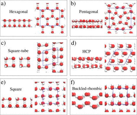
Figure 1: Double-layer ice structures. Side and top views of the (a) hexagonal (honeycomb), (b) pentagonal, (c) square-tube, (d) hexagonal-close-packed (HCP), (e) square and (f) buckled-rhombic double-layer structures. Red and white spheres represent oxygen and hydrogen atoms, respectively. The blue boxes in the top views show the unit cells used in the periodic DFT calculations. All the structure files are provided in the supplemental material si .

Structure	$E_{b}$ (meV/$\text{H}_{\text{2}}\text{O}$)	$A$ (Å2/$\text{H}_{\text{2}}\text{O}$)	$d$ (Å)
Hexagonal	548/575	10.10/9.76	2.85/2.80
Pentagonal	523/553	8.88/8.65	2.86/2.81
Square-tube	523/549	8.27/8.14	2.85/2.80
HCP	520/550	8.07/8.10	2.75/2.68
Square	511/538	8.49/8.40	2.86/2.80

Table 1: Binding energies (Eq. 1) and structural information of double-layer ice structures at ambient pressure without confinement. Larger values for $E_{b}$ suggest stronger binding. A is the lateral area per water molecule within a single layer. d is the average interlayer distance. Hexagonal represents the hexagonal honeycomb structure (Fig. 1a) and HCP represents the hexagonal-close-packed structure (Fig. 1d). Results using both the rPW86-vdW2 and optPBE-vdW functionals are reported (separated by a slash with rPW86-vdW2 in front).

III.2 Phase transitions of double-layer ice

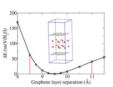
Figure 2: Total energy profile of water confined within two perfectly flat sheets of graphene fixed at the separations shown. The dashed lines show the confinement width regime examined in this study. The inset shows the structural model used for this specific set of calculations, which involves 16 water molecules in a hexagonal double-layer ice structure confined between two 32 carbon atom graphene sheets. On the energy scale the energy minimum is set to zero.

Examining the phase transitions at different confinement widths is desirable as the phase stability of confined ice is sensitive to the width of confinement Zangi and Mark (2003b, a); Giovambattista et al. (2009); Kastelowitz et al. (2010); Chen et al. (2016a). However, since a confinement that mimics graphene nanocapillaries is particularly interesting we first established what the appropriate confinement width for graphene is by examining the total energy of a double-layer ice film within two layers of graphene (Fig. 2). These calculations show that the optimal width of confinement is around 9.5 Å. This is the main reason our structure searches were performed at 9.5 Å confinement. However we also examined the stability of the relevant ice structures at a broader range of confinement. Fig. 3 shows the relative enthalpy with respect to the square-tube structure for confinements between 8.5 and 11.0 Å. At confinement widths of 8.5 and 9.0 Å, just a single transition is observed from the hexagonal to the HCP structure at about 0.5 GPa. At 9.5 Å the hexagonal structure is still the most stable structure below ca. 0.5 GPa. However, the square-tube structure becomes more stable than the HCP structure, leading to a new phase transition from the hexagonal to the square-tube structure. The HCP structure is slightly more stable than the square-tube at pressures above ca. 1.5 GPa and transforms to the buckled-rhombic structure at ca. 5 GPa. The transition between these two high density double-layer ice phases has also been identified in Ref. Corsetti et al., 2016b. As the width of confinement increases: (i) the stability of the hexagonal structure is not altered; (ii) the HCP and square-tube structures have very similar stability in a wide range of pressures, within which the square-tube structure is slightly preferred at wider confinements; and (iii) the transition pressure to the buckled-rhombic structure decreases, squeezing the stable region of the square-tube and HCP structures. Generally, the width dependency is strong for the HCP and buckled-rhombic structure whereas the relative stability of the hexagonal, pentagonal, square and square-tube phases barely changes at different confinement widths. This is not so surprising as the hexagonal, pentagonal, square and square-tube structures have the same number of interlayer hydrogen bonds and similar interlayer separations. The HCP structure is thinner and would be favored at narrow confinement whilst the buckled-rhombic structure is thicker and tends to appear in wider confinements.

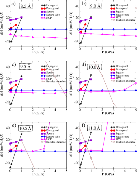
Figure 3: Enthalpies (relative to square-tube) of the double-layer ice structures as a function of lateral pressure for different confinement widths. These are from (a) to (f): 8.5, 9.0, 9.5, 10.0, 10.5 and 11.0 Å. The enthalpies of the hexagonal and square phases and the pentagonal phase are only shown up to 1 GPa and 0.5 GPa, respectively, because they are structurally unstable above this. The unstable structures and additional data showing the instability of these phases is included in the supplemental material.

The sequence of phase transitions at different confinement widths allows us to sketch a putative phase diagram for double-layer ice at 0 K as a function of pressure and confinement width (Fig. 4). In brief, double-layer ice appears as a hexagonal structure at low pressures ($\sim$ 0.5 GPa). This then transforms to the HCP structure at higher pressures for narrow confinement widths and to the square-tube structure for larger confinement widths. At higher pressures and larger confinement widths double-layer ice favors a buckled-rhombic structure.

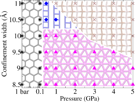
Figure 4: Schematic phase diagram of double-layer ice with respect to lateral pressure and confinement width. The phase diagram can be divided into four regions: (i) The hexagonal phase at low pressures; (ii) The HCP phase at high pressures and small confinement widths; (iii) The square-tube phase at pressures in the GPa regime and large confinement widths; (iv) The buckled-rhombic phase at high pressures and large confinement widths. The specific data points calculated are shown with the same set of symbols as in Fig. 3. Note that a logarithmic scale is used for pressure from 1 bar to 0.5 GPa and then a linear scale from 0.5 GPa to 5 GPa. We note that the enthalpy difference between the HCP and square-tube structures is so small that the boundary between these two phases is not well defined from our calculations, from which we see a region (0.5 - 1 GPa, 9.5 - 10 Å) that the hexagonal, HCP and square-tube structures are intermixed. However, due to the fact that the HCP has smaller interlayer distance and higher lateral density than the square-tube, the transition boundary between them is more likely to have a positive slope as shown in the figure.

III.3 Stability of double-layer square ice

Contrary to the monolayer, our predicted phase diagram for double-layer ice does not have a regime in which square ice is stable, whereas it is the only stable ice structure identified so far that matches the TEM images in graphene nanocapillaries . Our calculations reveal that irrespective of the confinement width the square structure is always at least ca. 20 meV/$\text{H}_{\text{2}}\text{O}$ less stable than the most stable structure (Fig. 3). This is consistent with another DFT study in which slightly different computational settings were used and double-layer square ice was also not identified as a stable phase Corsetti et al. (2016b). Intuitively the fact that the double-layer square phase is metastable is not so surprising by just comparing the square phase with the square-tube phase. Two steps can turn a double-layer square structure to a square-tube structure: changing the hydrogen ordering of the square phase and shifting the tubes by half a lattice unit. The re-ordering of hydrogen bonds is unlikely to cause a significant energy increase whereas the tube formation allows a further optimization step towards a more stable structure, the square-tube structure. However, due to the small energy differences between the different phases further calculations are needed to test this conclusion. Naturally it is reasonable to first consider the limitations of the simulations and to this end we specifically consider the following issues: (i) The accuracy of the underlying DFT calculations; (ii) The role of zero point energies; (iii) Finite temperature effects including harmonic and anharmonic phonon contributions; and (iv) Hydrogen ordering and the influence of configurational entropy. Each of these issues is addressed at a confinement width of 9.5 Å.

Sensitivity to exchange correlation functional: The first issue is the accuracy of DFT calculations specifically the XC functional used. The results reported so far have been obtained with the rPW86-vdW2 functional, which has proved to be accurate in predicting the binding energies of monolayer and bulk ice polymorphs Santra et al. (2013); Chen et al. (2016b). Nevertheless, it is also worth examining the results with other functionals. In Table 1 and Fig. 5a we report the binding energy, lattice parameter and enthalpy calculated using the optPBE-vdW functional. As shown in Fig. 5a, although the two functionals differ in their prediction of absolute binding energies and lattice parameters, the relative enthalpies between different phases mostly agree. Importantly, the difference between the square structure and the stable structures are consistent for these two functionals. Specifically at 1 GPa, the pressure regime at which square ice is estimated to form Algara-Siller et al. (2015a), the square-tube structure has a lower enthalpy by ca. 19 meV/$\text{H}_{\text{2}}\text{O}$ than the square structure.

There are, of course, many other XC functionals we could consider Gillan et al. (2016). Focusing on 1 GPa we have explored how several other functionals perform, including those with a different treatment of van der Waals and a hybrid exact exchange functional. The key results are given in Table 2. Overall we find that the difference between the square-tube and square structure is not very sensitive to the choice of XC functional and for all functionals square-tube is ca. 20 meV/$\text{H}_{\text{2}}\text{O}$ more stable than the square structure at 1 GPa. The apparent insensitivity to the XC functional can be further shown by the decomposition of enthalpy in Table 2.

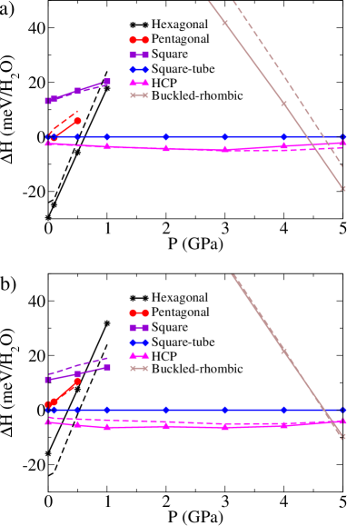
Figure 5: (a) Comparison of the relative enthalpies obtained with the optPBE-vdW (solid line) and rPW86-vdW2 (dashed lines) functionals. (b) Comparison of the relative enthalpies obtained from rPW86-vdW2 with (solid line) and without (dashed lines) zero point energy (ZPE). ZPEs have been calculated as, $E_{\text{ZPE}}=\sum_{i=1}^{i=N}\frac{1}{2}\hbar\omega_{\Gamma,i}$ where $\omega_{\Gamma,i}$ is the $i$th gamma point vibrational frequency calculated using the finite displacement method, and $\hbar$ is the reduced Planck constant, and N is the number of vibrational modes.

Methods	$\Delta H$	$\Delta E_{\text{ice}}^{\text{tot}}$	$\Delta E_{\text{confinement}}$	$\Delta(\text{P}\times\text{A}\times\text{h})$
rPW86-vdW2	19	14	0	5
optPBE-vdW	20	15	0	5
optB88-vdW	24	18	0	6
PBE+vdW(TS)	23	16	0	7
HSE+vdW(TS)	25	19	0	6

Table 2: Stability of the square-tube and double-layer square structures at 1 GPa calculated using different XC functionals at a confinement width of 9.5 Å. $\Delta H$, $\Delta E_{\text{ice}}^{\text{tot}}$, $\Delta E_{\text{confinement}}$ and $\Delta(P\times A\times h)$ are differences between the square and the square-tube structure for energy terms as defined in Eqs. 1 and 2. All values are reported in units of meV/$\text{H}_{\text{2}}\text{O}$.

Role of zero point energies: Since we consider small energy differences between the various phases it is possible that differences in zero point energy (ZPE) could tip the balance in stability between them. Therefore we computed the ZPE of relevant phases within the harmonic approximation. As shown in Fig. 5b no significant changes in phase transitions have been identified when ZPEs are accounted for. Specifically, comparing the enthalpy of the square structure and the square-tube structure at 1 GPa, the relative stability of the square structure is slightly increased by ca. 4 meV/$\text{H}_{\text{2}}\text{O}$.

Finite temperatures: Considering that the experiments from which square ice has been suggested have been carried out at room temperature Algara-Siller et al. (2015a), it is also important to evaluate the influence of finite temperature. Therefore, the free energy instead of the enthalpy should be calculated. As a first step the phonon free energy has been calculated at the harmonic level as, $E_{\text{vib}}=\int\hbar\omega[\frac{1}{2}+\frac{1}{\text{exp}(\hbar\omega/k_{B}T)-1}]g(\omega)d\omega$, where $g(\omega)$ is the phonon density of states (Fig. 6), $k_{B}$ the Boltzmann constant and $T$ the temperature. At 300 K the phonon free energy of the square structure is 6 meV/$\text{H}_{\text{2}}\text{O}$ less than that of the square-tube structure. Thus finite temperature effects increase the stability of the square structure, and even though the energy difference between the square and square-tube structures is very small, the square-tube structure remains marginally more stable.

Role of anharmonic effects: It is also possible that anharmonic phonon effects at finite temperature alter the stability of ice structures. Recently Engel et al. found that it can result in a difference of 6.5$\pm$3.1 meV/$\text{H}_{\text{2}}\text{O}$ for bulk ice Ih and Ic, which is large enough to explain the difference between harmonic theories and experiments Engel et al. (2015). They also showed that the anharmonic contribution mainly comes from the vibrational modes at high frequencies that are related to the motion of hydrogen atoms. Therefore, we carried out ab initio molecular dynamics simulations at 300 K for both the square-tube and square structures. Instead of accurately computing the challenging anharmonic free energy, here we try to estimate the influence of anharmonic effects qualitatively from these molecular dynamics simulations. Fig. 6a shows the distribution of OH bond lengths, which reflects the different types of hydrogen bonds in the two structures. The phonon density of states of these high frequency modes calculated from these trajectories are shown in Fig. 6b, where no significant difference is observed. We can also do the integration using the harmonic phonon free energy equation with these phonon density of states, which further shows that they are very similar as the integration gives a vanishing difference. Therefore, these simulations indicate that the anharmonic contribution is unlikely to alter the relative stability of the square and the square-tube structures.

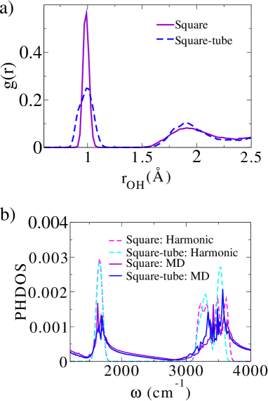
Figure 6: (a) Distribution of OH bond length for the square and square-tube structures as obtained from ab initio molecular dynamics simulations at 300 K. (b) Phonon density of states for the square and square-tube structures. Dashed lines: harmonic phonon density of states using the finite displacement method. The calculation was performed with a $2\times 2\times 1$ supercell and a $8\times 8\times 1$ grid in the phonon zone using the Phonopy package Togo and Tanaka (2015). Solid lines: phonon density of states calculated from ab initio molecular dynamics at 300 K.

Role of hydrogen ordering: In the discussion above the lowest enthalpy square and square-tube structures are compared. It is also important to consider how our conclusions at finite temperatures would be affected by the configurational entropy of hydrogen ordering (different distributions of hydrogen atoms within the same lattice of oxygen atoms), which is important in ice Salzmann et al. (2006, 2016). A transition from the square-tube structure to the HCP structure driven by configurational entropy has been predicted in Ref. Corsetti et al., 2016b. Here the possible configurations of different hydrogen distributions of the square and the square-tube structure are counted and the configurational entropy is estimated as $S=k_{B}ln\Omega$, where $\Omega$ is the number of possible states. Following the Bernal-Fowler and Pauling ice rules Bernal and Fowler (1933); Pauling (1935), we impose three rules to the square phase: (i) hydrogen atoms locate in or between the two layers; (ii) half of the water molecules only bond to neighbors within the same layer, the other half form one hydrogen bond within the layer and one hydrogen bond with the other layer; and (iii) between each oxygen atom pair there should be no more than one hydrogen atom. This leads to $\Omega_{square}=[C_{4}^{2}\times(C_{4}^{1})^{8}]^{1/8}\times(3/4)^{2}$. For the square-tube phase the rules are: (i) no hydrogen atoms are allowed outside of the tube; (ii) cells must be connected along the tube by more than (1/2) hydrogen bonds per water molecule; and (iii) between each oxygen atom pair there should be no more than one hydrogen atom. This leads to $\Omega_{square-tube}=(C_{8}^{4})^{3/8}\times(3/4)^{2}$. The contribution to the free energy difference between these two phases is $\Delta F\approx 0.02k_{B}T$ ($<$ 1 meV/$\text{H}_{\text{2}}\text{O}$), which is negligible compared to the difference between the square and square-tube structures. Although this estimate is crude and is based on the assumption that all possible hydrogen ordered states are degenerate, it suggests that configurational entropy effects are unlikely to alter the relative stability of the two structures significantly.

In this section we have addressed issues including the sensitivity of the results to the XC functional, ZPE, harmonic and anharmonic phonon free energies, and configurational entropy. There are other issues not addressed which might also be important. For instance, the presence of real graphene instead of a confining potential, the finite size of the ice structures observed in the experiments and the role of edges. We believe these effects will not affect our conclusions significantly because: (i) The graphene is incommensurate with the ice and the interaction between graphene and water molecules is not very sensitive to the orientation and lateral position of water molecules, which we have shown in our previous study Chen et al. (2016a). (ii) More hydrogen bonds break at the edge of the square structure than the square-tube structure. Thus, on the basis of our calculations, we conclude that double-layer square ice is a metastable phase across a wide range of confinement widths and pressures. Interestingly, our previous work found that monolayer square ice is a stable phase Chen et al. (2016a, b), which lends support to the experimental observations of square ice Algara-Siller et al. (2015a). Therefore, although we find double-layer square ice is metastable, it is possible that it forms as the growth of a metastable double-layer phase assisted by the presence of a stable monolayer. The influence of crystal growth kinetics and nucleation of square ice under confinement would therefore be an interesting issue to explore in future work. Experimentally, some well controlled annealing experiments could also be informative and help to establish if square ice is metastable. Zhou et al. questioned the observations of square ice from a different perspective suggesting that the confined material is layers of NaCl instead of ice Zhou et al. (2015); Algara-Siller et al. (2015b); Wang et al. (2015). Such a concern also calls for further experimental and theoretical investigations of both confined water and confined NaCl.

IV summary

In summary, on the basis of DFT calculations a phase diagram of double-layer ice as a function of pressure and confinement width at 0 K is predicted. Complementary to our previous studies on monolayer ice Chen et al. (2016a, b), this study shows an interesting change of the phase diagram from monolayer to double-layer ice in confinement due to the presence of interlayer hydrogen bonds. For monolayer ice, a pentagonal and a square structure appear in the GPa regime, whereas for double-layer ice the pentagonal and square structures are metastable and in the GPa regime double-layer ice favours HCP and square-tube structures. Beyond the general insights on the phase diagram of confined ice, we have performed extensive calculations focusing on the double-layer square ice, which has been a matter of debate recently between experiment and theory. Our results suggest that the double-layer square ice is a metastable phase.

Supplemental Material

This supplemental material contains: the confining potential at different widths (Fig. S1); additional enthalpy data and structures in Fig. SS2 and Fig. S3; and structure files for phases reported in the main text.

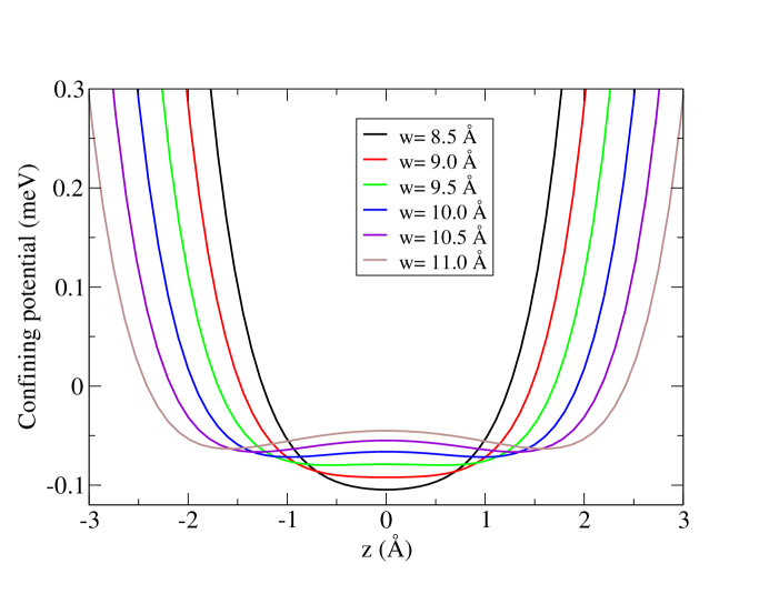
Figure S1: Confining potential at different widths.

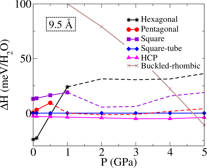
Figure S2: Enthalpies (relative to ST) of the double-layer ice structures as a function of lateral pressure at a confinement width of 9.5 Å. Solid lines with filled symbols are the same as Fig. 3(c). Dashed lines show the enthalpy of the structures obtained via structure optimisation starting with the hexagonal, pentagonal, and square phases at high pressure. The corresponding structures are shown in Fig. S2. The data points of the dashed lines are at 1, 2, 3, 4, and 5 GPa. We note that the small regime where the red dashed line has the lowest enthalpy does not indicate that we should have a new phase there. The red dashed line is the ST structure, with a larger unit cell and thus a slightly different hydrogen ordering.

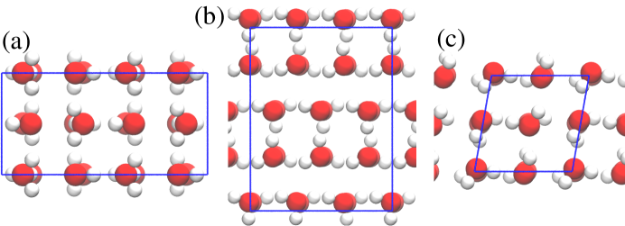
Figure S3: The structures corresponds to the dashed lines in Fig.  S1. (a) A square structure, with a different unit cell and hydrogen ordering, that comes from optimising the hexagonal phase at 2 GPa. (b) A ST structure, with a different unit cell and hydrogen ordering, that comes from optimising the pentagonal phase at 1 GPa. (c) A tilted square structure that comes from optimising the square phase at 2 GPa. Same structures were seen at higher pressures up to 5 GPa.

References

- Algara-Siller et al. (2015a) G. Algara-Siller, O. Lehtinen, F. C. Wang, R. R. Nair, U. Kaiser, H. A. Wu, A. K. Geim, and I. V. Grigorieva, Nature 519, 443 (2015a).
- Zhou et al. (2015) W. Zhou, K. Yin, C. Wang, Y. Zhang, T. Xu, A. Borisevich, L. Sun, J. C. Idrobo, M. F. Chisholm, S. T. Pantelides, R. F. Klie, and A. R. Lupini, Nature 528, E1 (2015).
- Algara-Siller et al. (2015b) G. Algara-Siller, O. Lehtinen, and U. Kaiser, Nature 528, E3 (2015b).
- Wang et al. (2015) F. C. Wang, H. A. Wu, and A. K. Geim, Nature 528, E3 (2015).
- Chen et al. (2016a) J. Chen, G. Schusteritsch, C. J. Pickard, C. G. Salzmann, and A. Michaelides, Physical Review Letters 116, 025501 (2016a).
- Corsetti et al. (2016a) F. Corsetti, P. Matthews, and E. Artacho, Scientific Reports 6, 18651 (2016a).
- Corsetti et al. (2016b) F. Corsetti, J. Zubeltzu, and E. Artacho, Physical Review Letters 116, 085901 (2016b).
- Roman and Groß (2016) T. Roman and A. Groß, The Journal of Physical Chemistry C 120, 13649 (2016).
- Chen et al. (2016b) J. Chen, A. Zen, J. G. Brandenburg, D. Alfè, and A. Michaelides, Physical Review B 94, 220102 (2016b).
- Berendsen et al. (1987) H. J. C. Berendsen, J. R. Grigera, and T. P. Straatsma, The Journal of Physical Chemistry 91, 6269 (1987).
- Jorgensen et al. (1983) W. L. Jorgensen, J. Chandrasekhar, J. D. Madura, R. W. Impey, and M. L. Klein, The Journal of Chemical Physics 79, 926 (1983).
- Lee et al. (2010) K. Lee, E. D. Murray, L. Kong, B. I. Lundqvist, and D. C. Langreth, Physical Review B 82, 081101 (2010).
- Koga et al. (1997) K. Koga, X. C. Zeng, and H. Tanaka, Physical Review Letters 79, 5262 (1997).
- Koga et al. (2000) K. Koga, H. Tanaka, and X. C. Zeng, Nature 408, 564 (2000).
- Zangi and Mark (2003a) R. Zangi and A. E. Mark, The Journal of Chemical Physics 119, 1694 (2003a).
- Giovambattista et al. (2009) N. Giovambattista, P. J. Rossky, and P. G. Debenedetti, Physical Review Letters 102, 050603 (2009).
- Han et al. (2010) S. Han, M. Y. Choi, P. Kumar, and H. E. Stanley, Nature Physics 6, 685 (2010).
- Johnston et al. (2010) J. C. Johnston, N. Kastelowitz, and V. Molinero, The Journal of Chemical Physics 133, 154516 (2010).
- Kastelowitz et al. (2010) N. Kastelowitz, J. C. Johnston, and V. Molinero, The Journal of Chemical Physics 132, 124511 (2010).
- Bai and Zeng (2012) J. Bai and X. C. Zeng, Proceedings of the National Academy of Sciences 109, 21240 (2012).
- Giovambattista et al. (2012) N. Giovambattista, P. Rossky, and P. Debenedetti, Annual Review of Physical Chemistry 63, 179 (2012).
- Zhao et al. (2014a) W.-H. Zhao, L. Wang, J. Bai, L.-F. Yuan, J. Yang, and X. C. Zeng, Accounts of Chemical Research 47, 2505 (2014a).
- Lu et al. (2014) Q. Lu, J. Kim, J. D. Farrell, D. J. Wales, and J. E. Straub, The Journal of Chemical Physics 141, 18C525 (2014).
- Sobrino Fernandez Mario et al. (2015) M. Sobrino Fernandez Mario, M. Neek-Amal, and F. M. Peeters, Physical Review B 92, 245428 (2015).
- Zubeltzu et al. (2016) J. Zubeltzu, F. Corsetti, M. V. Fernández-Serra, and E. Artacho, Physical Review E 93, 062137 (2016).
- Pickard and Needs (2011) C. J. Pickard and R. J. Needs, Journal of Physics: Condensed Matter 23, 053201 (2011).
- Kresse and Furthmüller (1996) G. Kresse and J. Furthmüller, Physical Review B 54, 11169 (1996).
- Kresse and Joubert (1999) G. Kresse and D. Joubert, Physical Review B 59, 1758 (1999).
- Klimeš et al. (2011) J. Klimeš, D. R. Bowler, and A. Michaelides, Physical Review B 83, 195131 (2011).
- Santra et al. (2013) B. Santra, J. Klimeš, A. Tkatchenko, D. Alfè, B. Slater, A. Michaelides, R. Car, and M. Scheffler, The Journal of Chemical Physics 139, 154702 (2013).
- Klimeš et al. (2010) J. Klimeš, D. R. Bowler, and A. Michaelides, Journal of Physics: Condensed Matter 22, 022201 (2010).
- Perdew et al. (1996) J. P. Perdew, K. Burke, and M. Ernzerhof, Physical Review Letters 77, 3865 (1996).
- Heyd et al. (2003) J. Heyd, G. E. Scuseria, and M. Ernzerhof, The Journal of Chemical Physics 118, 8207 (2003).
- Heyd et al. (2006) J. Heyd, G. E. Scuseria, and M. Ernzerhof, The Journal of Chemical Physics 124, 219906 (2006).
- Tkatchenko and Scheffler (2009) A. Tkatchenko and M. Scheffler, Physical Review Letters 102, 073005 (2009).
- Ma et al. (2011) J. Ma, A. Michaelides, D. Alfè, L. Schimka, G. Kresse, and E. Wang, Physical Review B 84, 033402 (2011).
- (37) See Supplemental Material for additional data and structure files.
- Note (1) , , and are the calculated lateral (x and y direction) diagonal stress tensor elements for the slab/vacuum model, is the length of the cell in the out-of-plane direction. In the calculation and are conserved quantities, the calculation of the enthalpy is independent of the definition of . Therefore, the shape of the phase diagram is not affected by the definition. However, the definition of does affect the values of the transition pressures predicted. Our definition indicates an upper limit of layer height (width of confinement), corresponding to a lower limit of transition pressures. Assuming the lower limit of width is ( = 9.5) the upper limit of the transition pressures are about 1.5 times larger.
- Nosé (1984) S. Nosé, The Journal of Chemical Physics 81, 511 (1984).
- Witek and Buch (1999) H. Witek and V. Buch, The Journal of Chemical Physics 110, 3168 (1999).
- Kimmel et al. (2009) G. A. Kimmel, J. Matthiesen, M. Baer, C. J. Mundy, N. G. Petrik, R. S. Smith, Z. Dohnálek, and B. D. Kay, Journal of the American Chemical Society 131, 12838 (2009).
- Zhao et al. (2014b) W.-H. Zhao, J. Bai, L.-F. Yuan, J. Yang, and X. C. Zeng, Chemical Science 5, 1757 (2014b).
- Sobrino Fernández et al. (2016) M. Sobrino Fernández, F. M. Peeters, and M. Neek-Amal, Physical Review B 94, 045436 (2016).
- Zangi and Mark (2003b) R. Zangi and A. E. Mark, Physical Review Letters 91, 025502 (2003b).
- Note (2) The lateral lattice constant and pressure of the square ice calculated are in agreement with the TEM measurements of lattice constant and pressure estimate. The lattice constant calculated using the rPW86-vdW2 functional at 1 GPa is 2.82 Å, and likewise a 2.83 Å lattice constant predicts a pressure of 0.91 GPa. There are a few aspects that need to be noted: (i) Thermal expansion is not considered; (ii) The estimated pressure in the experiments is based on a simple model whose accuracy is not clear; (iii) The relation between the lattice constant and pressure depends on the functional used, for instance the optPBE-vdW functional gives a lateral pressure of 0.65 GPa with a lattice constant of 2.83 Å; (iv) The relation between the lattice constant and pressure depends to some extent on the definition of lateral pressure, or in other words, the definition of the layer height. For double-layer ice our definition might underestimate the pressure, whereas the upper limit of pressure is about 50% larger as noted above.
- Gillan et al. (2016) M. J. Gillan, D. Alfè, and A. Michaelides, The Journal of Chemical Physics 144, 130901 (2016).
- Engel et al. (2015) E. A. Engel, B. Monserrat, and R. J. Needs, Physical Review X 5, 021033 (2015).
- Togo and Tanaka (2015) A. Togo and I. Tanaka, Scr. Mater. 108, 1 (2015).
- Salzmann et al. (2006) C. G. Salzmann, P. G. Radaelli, A. Hallbrucker, E. Mayer, and J. L. Finney, Science 311, 1758 (2006).
- Salzmann et al. (2016) C. G. Salzmann, B. Slater, P. G. Radaelli, J. L. Finney, J. J. Shephard, M. Rosillo-Lopez, and J. Hindley, The Journal of Chemical Physics 145, 204501 (2016).
- Bernal and Fowler (1933) J. D. Bernal and R. H. Fowler, The Journal of Chemical Physics 1, 515 (1933).
- Pauling (1935) L. Pauling, Journal of the American Chemical Society 57, 2680 (1935).