On the bound states of magnetic Laplacians on wedges

Abstract.

This paper is mainly inspired by the conjecture about the existence of bound states for magnetic Neumann Laplacians on planar wedges of any aperture $\phi\in(0,\pi)$. So far, a proof was only obtained for apertures $\phi\lesssim 0.511\pi$. The conviction in the validity of this conjecture for apertures $\phi\gtrsim 0.511\pi$ mainly relied on numerical computations. In this paper we succeed to prove the existence of bound states for any aperture $\phi\lesssim 0.583\pi$ using a variational argument with suitably chosen test functions. Employing some more involved test functions and combining a variational argument with computer-assistance, we extend this interval up to any aperture $\phi\lesssim 0.595\pi$. Moreover, we analyse the same question for closely related problems concerning magnetic Robin Laplacians on wedges and for magnetic Schrödinger operators in the plane with $\delta$-interactions supported on broken lines.

1. Introduction

Our first motivation comes from the problem of finding the ground state energy for the magnetic Neumann Laplacian, with a large magnetic field, on a bounded domain. This problem arises in the analysis of the Ginzburg-Landau equation in the regime of onset superconductivity in a surface, occurring when the intensity of an exterior magnetic field decreases from a large, critical value; see e.g.  [FH09, J01, LP99a], the monograph [FH], and the references therein.

Large field values for the magnetic Laplacian are equivalent, via scaling, to the semi-classical limit of the magnetic Schrödinger operators. In this limit, the magnetic Neumann Laplacian on a wedge emerges, after some derivation, as a model in the problem for domains with corners. Notably, spectral properties of this model operator are manifested in the semi-classical asymptotic expansion for the ground state eigenvalue of the initial magnetic Schrödinger operator on such a cornered domain; see e.g.  [BDP16, BF07, J01, P13] and the monographs [FH, R] for details. This mathematical problem resonates with the recent interest in surface superconductivity in presence of corners; see [CG17] and the references therein.

Some results about magnetic Schrödinger operators on domains with corners in the semi-classical limit [BDP16, R] have been proven assuming that certain spectral properties of magnetic Neumann Laplacians on wedges are valid. However, rigorous proofs of these properties are missing and only numerical evidences supporting them are available. The existence of bound states for any aperture in the interval $(0,\pi)$ is a prominent open problem of this type.

A similar question can be asked if the Neumann condition at the boundary is replaced by a Robin one, a problem which has recently gained attention [FRTS16, GKS16, KN15]. Moreover, one can study in the same line magnetic Schrödinger operators in the plane with a singular interaction of $\delta$-type supported by a wedge type structure, namely a broken line consisting of two half-lines meeting at the angle $\phi\in(0,\pi)$. We know that in the absence of the magnetic field such a system has a non-void discrete spectrum [EI01], and one asks whether this property persists in the presence of the magnetic field. Singular Schrödinger operators of this type are used to model leaky quantum wires and, apart of a few results [EY02], not much is known about their properties in the magnetic case [E08, Problem 7.15].

In the present paper, we study the existence of bound states for magnetic Laplacians on wedge-type structures with the homogeneous magnetic field and with both Robin and $\delta$ boundary conditions. These operators are fully characterized by the strength $\beta\in{\mathbb{R}}$ of the surface interaction and the opening angle $\phi\in(0,\pi)$ of the wedge. Making use of the min-max principle with suitable test functions we prove, for both boundary conditions, existence of bound states for sub-domains of the parametric space $(\phi,\beta)$. In the Robin setting, we put a particular emphasis on the case $\beta=0$, corresponding to the Neumann boundary condition. In this case, we analytically prove the existence of a bound state up to $\phi\lesssim 0.583\pi$. This is a notable improvement with respect to the previously known limit, $\phi\lesssim 0.511\pi$; cf.  [B03, B05, J01, Pa02]. Using more sophisticated test functions and additionally involving computer-assistance we managed to increase this limit up to $\phi\lesssim 0.595\pi$. We emphasize that this computer-assistance is different in nature from the numerical analysis in [BDMV06]. In fact, it is only needed to avoid dealing with tedious formulae and that the whole analysis can be, in principle, performed analytically.

The paper is organized as follows. In Section 2 we describe the geometric setting, define the Hamiltonians, and provide the notation used throughout the rest of the paper. In Section 3 we formulate and discuss the main results obtained in the paper. These results are proved in the two following sections: in Section 4 we treat the magnetic Neumann and Robin Laplacians on wedges, and in Section 5 the $\delta$-interaction on a broken line in the presence of a homogeneous magnetic field. Finally, in Appendix A we obtain variational characterisations for the bottoms of the essential spectra and explore their additional useful properties.

2. Magnetic Hamiltonians on wedge-type structures

First, we describe the geometric setting. In what follows, by a wedge of an aperture $\phi\in(0,2\pi)$ we understand an unbounded domain in ${\mathbb{R}}^{2}$, which is defined in the polar coordinates $(r,\theta)$ by

(2.1) $$\Omega_{\phi}:=\big{\{}(r,\theta)\in{\mathbb{R}}_{+}\times{\mathbb{S}}^{1}\colon\theta\in(0,\phi)\big{\}}\subset{\mathbb{R}}^{2};$$

see Figure 1.

                              $\Omega_{\phi}$$\phi$

Figure 1. Wedge $\Omega_{\phi}$ with the aperture $\phi\in(0,2\pi)$.

Note that for any $\phi\in(0,\pi]$ the Euclidean plane ${\mathbb{R}}^{2}$ can be naturally split into the wedge $\Omega_{\phi}$ and the non-convex ‘wedge’ $\Omega_{2\pi-\phi}$, provided that the latter is rotated by the angle $\phi$ counterclockwise. The common boundary of these two wedges is the broken line $\Gamma_{\phi}\subset{\mathbb{R}}^{2}$ consisting of two half-lines meeting at the angle $\phi\in(0,\pi]$. The complementary angle $\pi-\phi$ can be viewed as the ‘deficit’ of the broken line $\Gamma_{\phi}$ from the straight line.

Next we note that, since the considered geometry is scale invariant, we may assume without loss of generality that our magnetic field, homogeneous and perpendicular to the plane, satisfies $B=1$. We select the gauge by choosing the vector potential $\mathbf{A}\colon{\mathbb{R}}^{2}\rightarrow{\mathbb{R}}^{2}$ as

$$\mathbf{A}(x_{1},x_{2})=\frac{1}{2}(-x_{2},x_{1})^{\top},\qquad x=(x_{1},x_{2})\in{\mathbb{R}}^{2},$$

and define the associated magnetic gradient by $\nabla_{\mathbf{A}}:={\mathsf{i}}\nabla+\mathbf{A}$.

To describe all the situations mentioned in the introduction simultaneously, let $\Omega\in\{\Omega_{\phi},{\mathbb{R}}^{2}\}$ be fixed, where $\Omega_{\phi}\subset{\mathbb{R}}^{2}$ is a wedge as in (2.1), and denote, for the sake of brevity, $\Gamma=\Gamma_{\phi}$. With this notation, we introduce the magnetic first-order Sobolev space on $\Omega$ by

(2.2) $$H^{1}_{\mathbf{A}}(\Omega):=\left\{u\in L^{2}(\Omega)\colon\nabla_{\mathbf{A}}u\in L^{2}(\Omega;{\mathbb{C}}^{2})\right\},$$

where $\nabla_{\mathbf{A}}$ is computed in the distributional sense; cf.  [LL01, §7.20] for details. Finally, we define our operator of interest in the Hilbert space $L^{2}(\Omega)$ with the boundary/coupling parameter $\beta\in{\mathbb{R}}$ as the self-adjoint operator associated via the first representation theorem [K, Thm. VI 2.1] to the closed, densely defined, semi-bounded, and symmetric quadratic form

(2.3) $$H^{1}_{\mathbf{A}}(\Omega)\ni u\mapsto\mathfrak{h}[u]:=\left\|\nabla_{\mathbf{A}}u\right\|^{2}_{L^{2}(\Omega;{\mathbb{C}}^{2})}-\beta\|u|_{\Gamma}\|^{2}_{L^{2}(\Gamma)},\\$$

where $u|_{\Gamma}$ stands for the trace of $u\in H^{1}_{\mathbf{A}}(\Omega)$ onto $\Gamma$; cf.  [McL, Thm. 3.38]. We denote the form $\mathfrak{h}$ in (2.3) for $\Omega=\Omega_{\phi}$ by $\mathfrak{h}_{{\rm R},\phi,\beta}$ and for $\Omega={\mathbb{R}}^{2}$ by $\mathfrak{h}_{\delta,\phi,\beta}$. The operators associated with the forms $\mathfrak{h}_{{\rm R},\phi,\beta}$ and $\mathfrak{h}_{\delta,\phi,\beta}$ will be denoted by ${\mathsf{H}}_{{\rm R},\phi,\beta}$ and by ${\mathsf{H}}_{\delta,\phi,\beta}$, respectively. For $\beta=0$ the operator ${\mathsf{H}}_{{\rm N},\phi}:={\mathsf{H}}_{{\rm R},\phi,0}$ corresponding to the form $\mathfrak{h}_{{\rm N},\phi}:=\mathfrak{h}_{{\rm R},\phi,0}$ is the classical magnetic Neumann Laplacian on the wedge $\Omega_{\phi}$, extensively studied, e.g. , in [B05, J01, P12, P13, P15], see also the monographs [FH, R] and the references therein. For $\beta\neq 0$ the operator ${\mathsf{H}}_{{\rm R},\phi,\beta}$ can be interpreted as the magnetic Robin Laplacian on $\Omega_{\phi}$ discussed e.g. in [K06]. Finally, the operator ${\mathsf{H}}_{\delta,\phi,\beta}$ can be seen as the magnetic Schrödinger operator with a $\delta$-interaction supported on the broken line $\Gamma$; cf.  [E08, EY02, Ož06].

The bottoms of the essential spectra for ${\mathsf{H}}_{{\rm R},\phi,\beta}$ and ${\mathsf{H}}_{\delta,\phi,\beta}$ are denoted by

(2.4) $$\Theta_{{\rm R},\beta}:=\inf\sigma_{\rm ess}({\mathsf{H}}_{{\rm R},\phi,\beta})\qquad\text{and}\qquad\Theta_{\delta,\beta}:=\inf\sigma_{\rm ess}({\mathsf{H}}_{\delta,\phi,\beta}).$$

In Theorem A.1 we provide the variational characterisations for $\Theta_{{\rm R},\beta}$ and $\Theta_{\delta,\beta}$ which will be used throughout the paper. For the major part of our discussion it is only important to know that these thresholds do not depend on the aperture $\phi\in(0,\pi]$ of the wedge. Note also that in the Neumann case, $\beta=0$, we have $\Theta_{0}:=\Theta_{{\rm R},0}\approx 0.5901$ according to [J01, Sec. II]. The constant $\Theta_{0}$ is usually referred to as de Gennes constant and is characterized via the lowest eigenvalue of the shifted harmonic oscillator on the half-line; cf.  Appendix A.

3. Main results

As indicated in the abstract, the results of this paper are mainly connected with and motivated by the conjecture  [FH, Conj. 4.4.1] (see also [B05, Rem. 2.4]), namely

(3.1) $$\boxed{\sigma_{\rm d}({\mathsf{H}}_{{\rm N},\phi})\cap(0,\Theta_{0})\neq\varnothing,\qquad\forall\,\phi\in(0,\pi),}$$

which has been so far only proven for $\phi\lesssim 0.511\pi$, see [J01, Prop. 2.11], [Pa02, Sec. 2], [B05, Prop. 2.5 and Prop. 4.2], and [B03, Rem. 5.4]. A survey of the known results can be found in [FH, Sec. 4.4]; see also [B03, Sec. 11.3] and [P12, Sec. 3.2] for further details. The validity of (3.1) for $\phi\gtrsim 0.511\pi$ is still open to the best of our knowledge, although numerical computations in [BDMV06] confirm it. In this context we prove the following results.

Theorem 3.1.

Let $\phi\in(0,\pi)$ and $\beta\in{\mathbb{R}}$ be fixed. Let the polynomial $P_{\phi,\beta}(x)$ of the 4-th degree be defined by

(3.2) $$P_{\phi,\beta}(x):=x^{4}\left(2\phi-\pi\tanh\left(\tfrac{\phi}{2}\right)\right)-8\Theta_{{\rm R},\beta}\phi x^{2}-16\beta\sqrt{\pi}x+8\phi.$$

If $\min_{x\in(0,\infty)}P_{\phi,\beta}(x)<0$, then $\sigma_{\rm d}({\mathsf{H}}_{{\rm R},\phi,\beta})\cap(-\infty,\Theta_{{\rm R},\beta})\neq\varnothing$ holds.

The method of the proof of Theorem 3.1 relies on the min-max principle, in which we use test functions given in the polar coordinates $(r,\theta)$ by

(3.3) $$u_{\star}(r,\theta)=e^{-ar^{2}/2}\exp\left({\mathsf{i}}cr\left[e^{\theta}-e^{\phi-\theta}\right]\right),\qquad a,c>0.$$

The statement then follows upon analytical optimization with respect to the parameters $a,c>0$. This particular choice of the test function is inspired by the proof of [J01, Prop. 2.11]. The main novelty consists in the choice of the angular-dependent coefficient in the imaginary exponent via the functional derivative, which makes the choice optimal within a certain class of test functions; cf.  Subsection 4.1 for details.

Computing $\Theta_{{\rm R},\beta}$ numerically and analysing the condition $\min_{x\in(0,\infty)}P_{\phi,\beta}(x)<0$ we show that at least one bound state for ${\mathsf{H}}_{{\rm R},\phi,\beta}$ below the threshold $\Theta_{{\rm R},\beta}$ exists for a region in the $(\phi,\beta)$-plane, plotted in Figure 2.

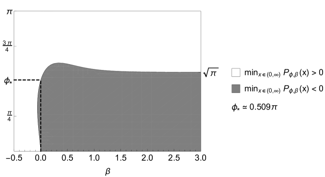
Figure 2. The region in the $(\phi,\beta)$-plane in which we prove existence of at least one bound state for ${\mathsf{H}}_{{\rm R},\phi,\beta}$ below $\Theta_{{\rm R},\beta}$.

Note that our results imply the existence of a bound state below the threshold of the essential spectrum for $\beta<0$ with small absolute value. We note that this cannot happen without the presence of a magnetic field.

For large $\beta>0$ we get the following consequence of Theorem 3.1 using the properties of $\Theta_{{\rm R},\beta}$, shown in Corollary A.2 (i) and (ii).

Corollary 3.2.

For any $\phi\in(0,\sqrt{\pi})$ (i.e. $\phi\lesssim 0.564\pi$),

$$\sigma_{\rm d}({\mathsf{H}}_{{\rm R},\phi,\beta})\cap(-\infty,\Theta_{{\rm R},\beta})\neq\varnothing,\qquad\text{for all}\,\,\beta>\frac{1}{2}\left(\frac{2\phi-\pi\tanh\left(\frac{\phi}{2}\right)}{\sqrt{\pi}-\phi}\right)^{\frac{1}{4}}.$$

In the case of Neumann boundary conditions ($\beta=0$) the expression for the polynomial in (3.2) simplifies and one can derive from Theorem 3.1 that $\sigma_{\rm d}({\mathsf{H}}_{{\rm N},\phi})\cap(-\infty,\Theta_{0})\neq\varnothing$ for all $\phi\lesssim 0.509\pi$. This interval of admissible apertures does not beat the previously known $\phi\lesssim 0.511\pi$. In order to obtain a better result we use test functions of a more general structure:

(3.4) $$u_{\star}(r,\theta)=e^{-ar^{2}/2}\exp\left({\mathsf{i}}\sum_{k=1}^{N}r^{k}b_{k}(\theta)\right),\qquad N\in{\mathbb{N}},$$

with the parameter $a>0$ and arbitrary real-valued functions $b_{k}\in C^{\infty}([0,\phi])$, $k=1,2,\dots,N$. Using functional derivative we observe that the optimal choice of $\{b_{k}\}_{k=1}^{N}$ is necessarily a solution of a certain system of linear second-order ordinary differential equations on the interval $[0,\phi]$ with constant coefficients. Employing the Ansatz (3.4) with $N=2$ we get the following result.

Theorem 3.3.

Let $s:=\sqrt{9-2\pi}$, $\mu_{1,2}:=\frac{s\pm 1}{\sqrt{4-\pi}}$, and $\nu_{1,2}:=\frac{\sqrt{4-\pi}(3-\pi\pm s)}{2(1\pm s)}$. If $\phi\in(0,\pi)$ is such that

(3.5) $$2\phi s\Theta_{0}^{2}\left[2\phi s-\mu_{1}^{2}\mu_{2}^{2}\left\{\nu_{1}\tanh\left(\tfrac{1}{2}\mu_{1}\phi\right)+\nu_{2}\tanh\left(\tfrac{1}{2}\mu_{2}\phi\right)\right\}\right]^{-1}>1,$$

then $\sigma_{\rm d}({\mathsf{H}}_{{\rm N},\phi})\cap(-\infty,\Theta_{0})\neq\varnothing$.

The condition (3.5) is satisfied, thus yielding the existence of at least one bound state for ${\mathsf{H}}_{{\rm N},\phi}$ below $\Theta_{0}$, for all $\phi\lesssim 0.583\pi$. This new limit is a significant improvement of the previously known interval $\phi\lesssim 0.511\pi$.

Using the Ansatz (3.4) with $N=4$ we confirm the validity of (3.1) for $\phi\lesssim 0.595\pi$. These computations are performed partly numerically, because making them fully analytical inevitably leads to tedious formulæ; see Subsection 4.2 for details. Performing computational experiments, we observe that the Ansatz (3.4) cannot be used to confirm the validity of (3.1) for $\phi\gtrsim 0.6\pi$.

As for the case of magnetic Schödinger operator ${\mathsf{H}}_{\delta,\phi,\beta}$ with $\delta$-interaction, we obtain the following result.

Theorem 3.4.

Let $\phi\in(0,\pi)$ and $\beta>0$ be fixed. Let $F_{\phi,\beta}(\cdot)$ be defined by

(3.6) $$F_{\phi,\beta}(x,y)=1+\frac{x^{4}}{4}-x^{2}\Theta_{\delta,\beta}-\beta x\pi^{-1/2}e^{-y^{2}\tan^{2}(\phi/2)}\left(1+{\rm erf}\,(y)\right).$$

If $\inf_{x,y\in(0,\infty)}F_{\phi,\beta}(x,y)<0$, then $\sigma_{\rm d}({\mathsf{H}}_{\delta,\phi,\beta})\cap(-\infty,\Theta_{\delta,\beta})\neq\varnothing$.

In order to prove Theorem 3.4, it is convenient to change the gauge by rotating and shifting the vector potential associated to the magnetic field. Equivalently, one can rotate and shift the broken line $\Gamma$, which is how we proceed. Specifically, we rotate the broken line $\Gamma$ by the angle $\pi/4-\phi/2$ counterclockwise and shift it by the vector $(-c,-c)^{\top}$, where $c>0$ is a parameter to be determined. Applying the min-max principle with the test function given in the polar coordinates $(r,\theta)$ by

(3.7) $$u_{\star}(r,\theta):=e^{-ar^{2}/2},\qquad a>0,$$

we obtain the claim upon analytical optimization with respect to the parameters $a,c>0$.

Computing $\Theta_{\delta,\beta}$ and analysing the condition $\inf_{(x,y)\in(0,\infty)}F_{\phi,\beta}(x,y)<0$ we observe the existence of at least one bound state for ${\mathsf{H}}_{\delta,\phi,\beta}$ below the threshold $\Theta_{\delta,\beta}$ for a region in the $(\phi,\beta)$-plane, plotted in Figure 3.

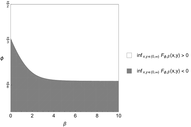
Figure 3. Region in the $(\phi,\beta)$-plane in which we prove the existence of bound states for ${\mathsf{H}}_{\delta,\phi,\beta}$ below $\Theta_{\delta,\beta}$.

.

Using the expansion of $\Theta_{\delta,\beta}$ in the limit $\beta\rightarrow 0+$ given in Corollary A.2 (iii) and a lower bound on $\Theta_{\delta,\beta}$ in Corollary A.2 (i) we get the following consequence of Theorem 3.4.

Corollary 3.5.

The following claims hold.

• For any $\phi\in\big{(}0,\frac{1}{3}\pi\big{]}$, $\sigma_{\rm d}({\mathsf{H}}_{\delta,\phi,\beta})\cap(-\infty,\Theta_{\delta,\beta})\neq\varnothing$ holds for all $\beta>0$ small enough.

• For any $\phi\in\big{(}0,\frac{1}{8}\pi\big{]}$, $\sigma_{\rm d}({\mathsf{H}}_{\delta,\phi,\beta})\cap(-\infty,\Theta_{\delta,\beta})\neq\varnothing$ holds for all $\beta>0$ large enough.

Finally, we point out that if we allow for homogeneous magnetic field of arbitrary intensity $B\in{\mathbb{R}}\setminus\{0\}$, then, by scaling, Corollary 3.5 yields the existence of at least one bound state below the threshold of the essential spectrum for the magnetic Schrödinger operators with $\delta$-interaction supported on $\Gamma$ of fixed strength $\beta>0$ and all sufficiently large or sufficiently small $|B|$.

Note that part of the results shown above are based on numerical analysis, as proving the validity of (3.1) for $\phi\lesssim 0.595\pi$ or the computation of the bottoms of the essential spectra $\Theta_{{\rm R},\beta}$ and $\Theta_{\delta,\beta}$. For these numerical solutions and minimizations we use the default Newton and quasi-Newton methods integrated in Wolfram Mathematica.

4. Neumann and Robin boundary conditions

In this section we consider the magnetic Neumann and Robin Laplacians on wedges. First, in Subsection 4.1 we prove Theorem 3.1 on the existence of bound states for ${\mathsf{H}}_{{\rm R},\phi,\beta}$ below the threshold $\Theta_{{\rm R},\beta}$ and its Corollary 3.2 for large $\beta>0$. In Subsection 4.2 we discuss improvements upon Theorem 3.1 for the case $\beta=0$ with the aid of the Ansatz (3.4). In particular, employing the Ansatz (3.4) with $N=2$ we prove Theorem 3.3.

4.1. Robin boundary conditions

We make use of a test function given in the polar coordinates $(r,\theta)$ by

(4.1) $$u_{\star}(r,\theta)=f(r)e^{{\mathsf{i}}b(r,\theta)}\in H^{1}_{\mathbf{A}}(\Omega_{\phi}),$$

where the functions $f\colon{\mathbb{R}}_{+}\rightarrow{\mathbb{R}}$ and $b\colon{\mathbb{R}}_{+}\times(0,\phi)\rightarrow{\mathbb{R}}$ will be chosen later. Substituting $u_{\star}$ into the functional

(4.2) $$H^{1}_{\mathbf{A}}(\Omega_{\phi})\mapsto{\mathcal{I}}[u]:=\mathfrak{h}_{{\rm R},\phi,\beta}[u]-\Theta_{{\rm R},\beta}\|u\|^{2}_{L^{2}(\Omega_{\phi})}$$

we obtain after elementary computations

(4.3) $${\mathcal{I}}[u_{\star}]=\int_{0}^{\phi}\int_{0}^{\infty}\left\{f(r)^{2}\left((\partial_{r}b)^{2}+\frac{(\partial_{\theta}b)^{2}}{r^{2}}-\partial_{\theta}b+\frac{r^{2}}{4}-\Theta_{{\rm R},\beta}-\frac{2\beta}{\phi r}\right)+(\partial_{r}f)^{2}\right\}r{\mathsf{d}}r{\mathsf{d}}\theta.$$

Now we are prepared to prove Theorem 3.1.

Proof of Theorem 3.1.

We fix $f$ and $b$ in (4.1) by $f(r)=e^{-ar^{2}/2}$ and $b(r,\theta)=rb_{1}(\theta)$, where $b_{1}(\theta)\in C^{\infty}([0,\phi])$ will be selected later. With this choice of $f$ and $b$ we rewrite ${\mathcal{I}}[u_{\star}]$ as

(4.4) $$\begin{split}{\mathcal{I}}[u_{\star}]&=\int_{0}^{\phi}\int_{0}^{\infty}re^{-ar^{2}}\left\{\left(b_{1}^{2}+(\partial_{\theta}b_{1})^{2}-r\partial_{\theta}b_{1}+\frac{r^{2}}{4}-\Theta_{{\rm R},\beta}-\frac{2\beta}{\phi r}\right)+a^{2}r^{2}\right\}{\mathsf{d}}r{\mathsf{d}}\theta\\ &=\int_{0}^{\infty}re^{-ar^{2}}{\mathsf{d}}r\int_{0}^{\phi}\left(b_{1}^{2}+(\partial_{\theta}b_{1})^{2}-\Theta_{{\rm R},\beta}\right){\mathsf{d}}\theta-\int_{0}^{\infty}r^{2}e^{-ar^{2}}{\mathsf{d}}r\int_{0}^{\phi}\partial_{\theta}b_{1}{\mathsf{d}}\theta\\ &\qquad\qquad\qquad\qquad\qquad\quad+\left(a^{2}\phi+\frac{\phi}{4}\right)\int_{0}^{\infty}r^{3}e^{-ar^{2}}{\mathsf{d}}r-2\beta\int_{0}^{\infty}e^{-ar^{2}}{\mathsf{d}}r.\end{split}$$

In what follows, we set ${\mathcal{E}}_{n}:=\int_{0}^{\infty}r^{n}e^{-ar^{2}}{\mathsf{d}}r$, $n\geq 0$. Using that (see [GR, Eqs. 3.461 (2), (3)])

(4.5) $${\mathcal{E}}_{0}=\frac{\pi^{1/2}}{2a^{1/2}},\qquad{\mathcal{E}}_{1}=\frac{1}{2a},\qquad{\mathcal{E}}_{2}=\frac{\sqrt{\pi}}{4a^{3/2}},\qquad{\mathcal{E}}_{3}=\frac{1}{2a^{2}},$$

we simplify the expression for ${\mathcal{I}}[u_{\star}]$ as

(4.6) $${\mathcal{I}}[u_{\star}]=\frac{1}{2a}\int_{0}^{\phi}\left(b_{1}^{2}+(\partial_{\theta}b_{1})^{2}\right){\mathsf{d}}\theta-\frac{\sqrt{\pi}}{4a^{3/2}}[b_{1}]_{0}^{\phi}+{\mathcal{J}}(a),$$

where

$$[b_{1}]_{0}^{\phi}=b_{1}(\phi)-b_{1}(0){\mathcal{J}}(a):=\frac{\phi}{2}-\frac{\Theta_{{\rm R},\beta}\phi}{2a}+\frac{\phi}{8a^{2}}-\beta\sqrt{\frac{\pi}{a}}.$$

Now we plug $b_{1}(\theta)=\alpha^{+}e^{\theta}+\alpha^{-}e^{-\theta}$ with $\alpha^{\pm}\in{\mathbb{R}}$ into the above expression for ${\mathcal{I}}[u_{\star}]$

$$\begin{split}{\mathcal{I}}[u_{\star}]&=\frac{1}{a}\int_{0}^{\phi}\left((\alpha^{+})^{2}e^{2\theta}+(\alpha^{-})^{2}e^{-2\theta}\right){\mathsf{d}}\theta-\frac{\sqrt{\pi}}{4a^{3/2}}\left(\alpha^{+}(e^{\phi}-1)+\alpha^{-}(e^{-\phi}-1)\right)+{\mathcal{J}}(a)\\ &=\frac{1}{2a}\left((\alpha^{+})^{2}(e^{2\phi}-1)+(\alpha^{-})^{2}(1-e^{-2\phi})\right)\\ &\qquad\qquad-\frac{\sqrt{\pi}}{4a^{3/2}}\left(\alpha^{+}(e^{\phi}-1)+\alpha^{-}(e^{-\phi}-1)\right)+{\mathcal{J}}(a).\end{split}$$

Let us further set $\alpha=\alpha^{+}$ and $\alpha^{-}=-e^{\phi}\alpha$ in the last expression

$${\mathcal{I}}[u_{\star}]=\frac{\alpha^{2}}{a}(e^{2\phi}-1)-\frac{\alpha\sqrt{\pi}}{2a^{3/2}}(e^{\phi}-1)+{\mathcal{J}}(a).$$

The latter can be viewed as a quadratic polynomial in $\alpha$. Minimising it with respect to $\alpha$ we obtain, with $x:=1/\sqrt{a}$,

$$\begin{split}{\mathcal{I}}[u_{\star}]&=-x^{4}\frac{\pi}{16}\frac{(e^{\phi}-1)^{2}}{e^{2\phi}-1}+{\mathcal{J}}(1/x^{2})\\ &=-x^{4}\frac{\pi}{16}\frac{(e^{\phi}-1)^{2}}{e^{2\phi}-1}-\frac{\Theta_{{\rm R},\beta}\phi x^{2}}{2}+\frac{\phi}{2}+\frac{x^{4}\phi}{8}-\beta\sqrt{\pi}x\\ &=x^{4}\left(\frac{\phi}{8}-\frac{\pi\tanh(\phi/2)}{16}\right)-\frac{\Theta_{{\rm R},\beta}\phi x^{2}}{2}+\frac{\phi}{2}-\beta\sqrt{\pi}x=\frac{P_{\phi,\beta}(x)}{16}.\end{split}$$

If $\min_{x\in(0,\infty)}P_{\phi,\beta}(x)<0$, then the min-max principle [RS4, Thm. XIII.2] yields the claim. ∎

The choice of the function $b_{1}$ in the proof of Theorem 3.1 relied on the functional derivative for the functional

$$C^{\infty}([0,\phi])\ni b_{1}\mapsto\frac{1}{2a}\int_{0}^{\phi}\left(b_{1}^{2}+(\partial_{\theta}b_{1})^{2}\right){\mathsf{d}}\theta-\frac{\sqrt{\pi}}{4a^{3/2}}[b_{1}]_{0}^{\phi}$$

appearing in (4.6). As a consequence of this procedure one gets that the optimal $b_{1}$ necessarily satisfies the linear second-order ordinary differential equation $b_{1}^{\prime\prime}(\theta)-b_{1}(\theta)=0$ on $[0,\phi]$ and the choice

(4.7) $$b_{1}(\theta)=\alpha^{+}e^{\theta}+\alpha^{-}e^{-\theta}$$

is simply the general solution of this ODE. The differential equation on $b_{1}$ itself is independent of $\beta$, but the parameter $\beta$ enters in the optimal choice of the constants $\alpha^{\pm}$ in (4.7). It can also be shown that the relation $\alpha^{-}=-e^{\phi}\alpha^{+}$ is necessarily satisfied by the optimal choice of $(\alpha^{+},\alpha^{-})$ for any $\beta$.

Next, we prove Corollary 3.2 on large values of $\beta$.

Proof of Corollary 3.2.

By Corollary A.2 (i) we have $\Theta_{{\rm R},\beta}\geq-\beta^{2}$ for $\beta>0$. Hence, substituting $x=1/\beta$ into $P_{\phi,\beta}(\cdot)$ we obtain that

$$P_{\phi,\beta}(1/\beta)\leq\beta^{-4}\left(2\phi-\pi\tanh\left(\frac{\phi}{2}\right)\right)+16\left(\phi-\sqrt{\pi}\right)<0,$$

for all $\beta>\frac{1}{2}\left(\frac{2\phi-\pi\tanh\left(\frac{\phi}{2}\right)}{\sqrt{\pi}-\phi}\right)^{\frac{1}{4}}$ and $\phi\in(0,\sqrt{\pi})$. Theorem 3.1 immediately yields the claim. ∎

4.2. Improvements in the Neumann case ($\beta=0$)

The result of Theorem 3.1 can be improved if we consider more involved classes of test functions of the form (3.4). In order to illustrate the idea we restrict our attention to the Neumann setting ($\beta=0$).

Proof of Theorem 3.3.

We employ test functions of the type (3.4) with $N=2$:

$$u_{\star}(r,\theta)=e^{-ar^{2}/2}\exp\left({\mathsf{i}}\left[rb_{1}(\theta)+r^{2}b_{2}(\theta)\right]\right),$$

where the real-valued functions $b_{1},b_{2}\in C^{\infty}([0,\phi])$ will be fixed later. Define the auxiliary functions

$$\begin{split}F_{1}(r,\theta)&:=(b_{1}(\theta))^{2}+4r^{2}(b_{2}(\theta))^{2}+4rb_{1}(\theta)b_{2}(\theta)+r^{2}(b^{\prime}_{2}(\theta))^{2}+(b_{1}^{\prime}(\theta))^{2}+2rb_{1}^{\prime}(\theta)b_{2}^{\prime}(\theta),\\ F_{2}(r,\theta)&:=-r^{2}b_{2}^{\prime}(\theta)-rb_{1}^{\prime}(\theta),\\ F_{3}(r)&:=\left(a^{2}+\frac{1}{4}\right)r^{2}-\Theta_{0}.\end{split}$$

For the sake of brevity, we introduce the notation $[b]_{0}^{\phi}:=b(\phi)-b(0)$ for a function $b\in C^{\infty}([0,\phi])$. Substituting $f(r)=e^{-ar^{2}/2}$, $b(r,\theta)=rb_{1}(\theta)+r^{2}b_{2}(\theta)$, and $\beta=0$ into (4.3) we get

(4.8) $$\begin{split}{\mathcal{I}}[u_{\star}]&=\int_{0}^{\phi}{\mathsf{d}}\theta\int_{0}^{\infty}re^{-ar^{2}}\left(F_{1}(r,\theta)+F_{2}(r,\theta)+F_{3}(r)\right){\mathsf{d}}r\\ &=\int_{0}^{\phi}\left[\frac{(b^{\prime}_{1}(\theta))^{2}}{2a}+\frac{(b^{\prime}_{2}(\theta))^{2}}{2a^{2}}+\frac{\sqrt{\pi}b_{1}^{\prime}(\theta)b_{2}^{\prime}(\theta)}{2a^{3/2}}\right]{\mathsf{d}}\theta\\ &\qquad+\int_{0}^{\phi}\left[\frac{(b_{1}(\theta))^{2}}{2a}+\frac{2(b_{2}(\theta))^{2}}{a^{2}}+\frac{\sqrt{\pi}b_{1}(\theta)b_{2}(\theta)}{a^{3/2}}\right]{\mathsf{d}}\theta\\ &\qquad\qquad\qquad\qquad\qquad\qquad\qquad-\frac{[b_{2}]_{0}^{\phi}}{2a^{2}}-\frac{\sqrt{\pi}[b_{1}]_{0}^{\phi}}{4a^{3/2}}+{\mathcal{J}}(a),\end{split}$$

where ${\mathcal{J}}(a):=\frac{\phi(4a^{2}+1-4a\Theta_{0})}{8a^{2}}$. Applying the functional derivative to ${\mathcal{I}}[u_{\star}]$ in (4.8), we find that the optimal choice of $b_{1}$ and $b_{2}$ constitutes a solution of the linear system of second-order ordinary differential equations with constant coefficients

(4.9) $$\begin{pmatrix}2a&\sqrt{a\pi}\\ \sqrt{a\pi}&2\\ \end{pmatrix}\begin{pmatrix}b_{1}^{\prime\prime}(\theta)\\ b_{2}^{\prime\prime}(\theta)\end{pmatrix}=\begin{pmatrix}2a&2\sqrt{a\pi}\\ 2\sqrt{a\pi}&8\\ \end{pmatrix}\begin{pmatrix}b_{1}(\theta)\\ b_{2}(\theta)\end{pmatrix}.$$

Integrating by parts, we simplify the expression for ${\mathcal{I}}[u_{\star}]$, with $b_{1},b_{2}$ satisfying (4.9),

(4.10) $${\mathcal{I}}[u_{\star}]=\left[\frac{b_{1}^{\prime}b_{1}}{2a}+\frac{b_{2}^{\prime}b_{2}}{2a^{2}}+\frac{(b_{1}^{\prime}b_{2}+b_{1}b_{2}^{\prime})\sqrt{\pi}}{4a^{3/2}}-\frac{b_{2}}{2a^{2}}-\frac{\sqrt{\pi}b_{1}}{4a^{3/2}}\right]_{0}^{\phi}+{\mathcal{J}}(a).$$

Further, denoting

$${\bf b}(\theta):=(b_{1}(\theta),b_{2}(\theta))^{\top},\qquad A:=\begin{pmatrix}\frac{4-2\pi}{4-\pi}&-\frac{4\sqrt{\pi}a^{-1/2}}{4-\pi}\\ \frac{2a^{1/2}\sqrt{\pi}}{4-\pi}&\frac{16-2\pi}{4-\pi}\\ \end{pmatrix},$$

we rewrite the system of differential equations (4.9) as

(4.11) $${\bf b}^{\prime\prime}(\theta)=A{\bf b}(\theta).$$

The eigenvalues and the corresponding eigenvectors of the matrix $A$ are given by

$$\lambda_{1,2}=\frac{10-2\pi\pm 2s}{4-\pi}\qquad{\bf c}_{1,2}=(a^{-1/2}c_{1,2},1)^{\top}=\left(\frac{-3\pm s}{\sqrt{a\pi}},1\right)^{\top},$$

where $s=\sqrt{9-2\pi}$. Hence, the general real-valued solution of the system (4.11) can be parametrised as

$${\bf b}(\theta)={\bf c}_{1}\chi_{1}(\theta)+{\bf c}_{2}\chi_{2}(\theta),\qquad\text{for}\,\,\,\,\chi_{j}(\theta):=\alpha_{j}^{+}e^{\mu_{j}\theta}+\alpha_{j}^{-}e^{-\mu_{j}\theta},\,\,\,j=1,2,$$

where $\mu_{1,2}=\sqrt{\lambda_{1,2}}=\frac{s\pm 1}{\sqrt{4-\pi}}$ and where $\alpha_{j}^{\pm}\in{\mathbb{R}}$ ($j=1,2$) are arbitrary constants. Introducing the shorthand notation $g_{x}:=e^{x\phi}-1$ for $x\in{\mathbb{R}}$, we find for $i,j\in\{1,2\}$

$$\begin{split}[\chi_{j}]_{0}^{\phi}&=\alpha_{j}^{+}g_{\mu_{j}}+\alpha_{j}^{-}g_{-\mu_{j}},\\ [\chi_{i}\chi_{j}^{\prime}]_{0}^{\phi}&=\mu_{j}\left[\alpha_{i}^{+}\alpha_{j}^{+}g_{\mu_{i}+\mu_{j}}-\alpha_{i}^{-}\alpha_{j}^{-}g_{-\mu_{i}-\mu_{j}}-\alpha_{i}^{+}\alpha_{j}^{-}g_{\mu_{i}-\mu_{j}}+\alpha_{i}^{-}\alpha_{j}^{+}g_{-\mu_{i}+\mu_{j}}\right].\end{split}$$

In view of ${\bf b}^{\prime}(\theta)={\bf c}_{1}\chi_{1}^{\prime}(\theta)+{\bf c}_{2}\chi_{2}^{\prime}(\theta)$, we also get

$$\begin{split}b_{1}^{\prime}b_{1}&=a^{-1}\big{[}c_{1}^{2}\chi_{1}^{\prime}\chi_{1}+c_{1}c_{2}(\chi_{1}^{\prime}\chi_{2}+\chi_{1}\chi_{2}^{\prime})+c_{2}^{2}\chi_{2}^{\prime}\chi_{2}\big{]},\\ b_{2}^{\prime}b_{2}&=\chi_{1}^{\prime}\chi_{1}+\chi_{1}^{\prime}\chi_{2}+\chi_{1}\chi_{2}^{\prime}+\chi_{2}^{\prime}\chi_{2},\\ b_{1}^{\prime}b_{2}&=a^{-1/2}\big{[}c_{1}(\chi_{1}^{\prime}\chi_{1}+\chi_{1}^{\prime}\chi_{2})+c_{2}(\chi_{2}^{\prime}\chi_{1}+\chi_{2}^{\prime}\chi_{2})\big{]}\\ b_{1}b_{2}^{\prime}&=a^{-1/2}\big{[}c_{1}(\chi_{1}\chi_{1}^{\prime}+\chi_{1}\chi_{2}^{\prime})+c_{2}(\chi_{2}\chi_{1}^{\prime}+\chi_{2}\chi_{2}^{\prime})\big{]}.\end{split}$$

Further, we introduce for $i,j\in\{1,2\}$ the constants

$$\gamma_{ij}:=\frac{c_{i}c_{j}}{2}+\frac{1}{2}+\frac{\sqrt{\pi}(c_{i}+c_{j})}{4}\qquad\text{and}\qquad\delta_{j}:=\frac{1}{2}+\frac{\sqrt{\pi}c_{j}}{4}=\frac{-1\pm s}{4}.$$

Hence, we can rewrite the functional in (4.10) as

$$\begin{split}{\mathcal{I}}[u_{\star}]&=\frac{1}{a^{2}}\left(\sum_{i,j=1}^{2}\gamma_{ij}[\chi_{i}\chi_{j}^{\prime}]_{0}^{\phi}-\delta_{1}[\chi_{1}]_{0}^{\phi}-\delta_{2}[\chi_{2}]_{0}^{\phi}\right)+{\mathcal{J}}(a)\\ &=\sum_{i,j=1}^{2}\frac{\gamma_{ij}\mu_{j}}{a^{2}}\left[\alpha_{i}^{+}\alpha_{j}^{+}g_{\mu_{i}+\mu_{j}}-\alpha_{i}^{-}\alpha_{j}^{-}g_{-\mu_{i}-\mu_{j}}-\alpha_{i}^{+}\alpha_{j}^{-}g_{\mu_{i}-\mu_{j}}+\alpha_{i}^{-}\alpha_{j}^{+}g_{-\mu_{i}+\mu_{j}}\right]\\ &\qquad\qquad\qquad-\sum_{j=1}^{2}\frac{\delta_{j}}{a^{2}}\big{(}\alpha_{j}^{+}g_{\mu_{j}}+\alpha_{j}^{-}g_{-\mu_{j}}\big{)}+{\mathcal{J}}(a).\end{split}$$

Analysing the above quadratic form with respect to the parameters $\alpha_{j}^{\pm}$, $j=1,2$, we conclude that the minimal value of ${\mathcal{I}}[u_{\star}]$ is attained at the vector $\alpha=(\alpha_{1},\alpha_{2})^{\top}=(\alpha_{1}^{+},\alpha_{1}^{-},\alpha_{2}^{+},\alpha_{2}^{-})^{\top}$ being the solution of the linear system of equations

(4.12) $$\begin{pmatrix}2\gamma_{11}\mu_{1}B_{11}&\gamma_{12}B_{12}\\ \gamma_{12}B_{12}^{*}&2\gamma_{22}\mu_{2}B_{22}\end{pmatrix}\begin{pmatrix}\alpha_{1}\\ \alpha_{2}\end{pmatrix}=\begin{pmatrix}\delta_{1}v_{1}\\ \delta_{2}v_{2}\end{pmatrix},$$

where the matrices $B_{11},B_{22},B_{12}$ and the vectors $v_{1},v_{2}$ are defined by

$$\begin{split}B_{jj}&:=\begin{pmatrix}g_{2\mu_{j}}&0\\ 0&-g_{-2\mu_{j}}\end{pmatrix},\qquad v_{j}:=\begin{pmatrix}g_{\mu_{j}}\\ g_{-\mu_{j}}\end{pmatrix},\qquad j=1,2,\\ B_{12}&:=\begin{pmatrix}(\mu_{1}+\mu_{2})g_{\mu_{1}+\mu_{2}}&(\mu_{1}-\mu_{2})g_{\mu_{1}-\mu_{2}}\\ (\mu_{2}-\mu_{1})g_{\mu_{2}-\mu_{1}}&-(\mu_{1}+\mu_{2})g_{-\mu_{1}-\mu_{2}}\end{pmatrix}.\end{split}$$

Solving the system (4.12), we find

$$\alpha_{j}^{\pm}=\frac{\mu_{1}^{2}\mu_{2}^{2}}{16\mu_{j}g_{\pm\mu_{j}}r_{j}s}\tanh\left(\tfrac{1}{2}\mu_{j}\phi\right),\qquad j=1,2,$$

with $r_{1,2}=-\frac{(\pm 1-s)}{2(3-\pi\pm s)}$. The value of the functional ${\mathcal{I}}[u_{\star}]$ for $\alpha\in{\mathbb{R}}^{4}$ as above is given by

(4.13) $$\begin{split}{\mathcal{I}}[u_{\star}]&=-\frac{x^{2}}{2}\sum_{j=1}^{2}\delta_{j}(\alpha_{j}^{+}g_{\mu_{j}}+\alpha_{j}^{-}g_{-\mu_{j}})+{\mathcal{J}}(1/x)\\ &=x^{2}\left[\frac{\phi}{8}-\frac{\mu_{1}^{2}\mu_{2}^{2}}{16s}\left(\nu_{1}\tanh\left(\tfrac{1}{2}\mu_{1}\phi\right)+\nu_{2}\tanh\left(\tfrac{1}{2}\mu_{2}\phi\right)\right)\right]-x\frac{\phi\Theta_{0}}{2}+\frac{\phi}{2},\end{split}$$

where $x:=1/a$ and $\nu_{j}=\frac{\delta_{j}}{\mu_{j}r_{j}}=\frac{\sqrt{4-\pi}}{2}\frac{3-\pi\pm s}{1\pm s}$, $j=1,2$. The expression on the right-hand side in (4.13) is a quadratic polynomial in $x$. Minimizing it with respect to the parameter $x>0$ we find that the minimal value equals

$${\mathcal{I}}[u_{\star}]=\frac{\phi}{2}-\phi^{2}s\Theta_{0}^{2}\left[2\phi s-\mu_{1}^{2}\mu_{2}^{2}\left\{\nu_{1}\tanh\left(\tfrac{1}{2}\mu_{1}\phi\right)+\nu_{2}\tanh\left(\tfrac{1}{2}\mu_{2}\phi\right)\right\}\right]^{-1}.$$

Analysing numerically the above expression, we obtain that ${\mathcal{I}}[u_{\star}]<0$ for all $\phi<\phi_{\star}\approx 0.583\pi$; cf.  Figure 4.

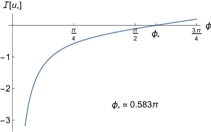
Figure 4. The graph of the right-hand side in (4.4) as a function of $\phi$.

The claim follows from the min-max principle. ∎

Furthermore, we try test functions of the type (3.4) with $N=3$

(4.14) $$u_{\star}(r,\theta)=e^{-ar^{2}/2}\exp\left({\mathsf{i}}\left[rb_{1}(\theta)+r^{2}b_{2}(\theta)+r^{3}b_{3}(\theta)\right]\right),$$

where the optimal choice of the real-valued functions $b_{1},b_{2},b_{3}\in C^{\infty}([0,\phi])$ satisfies the system of ordinary differential equations

$$\begin{pmatrix}2a&\sqrt{a\pi}&2\\ 2a\sqrt{\pi}&4\sqrt{a}&3\sqrt{\pi}\\ 4a&3\sqrt{a\pi}&8\end{pmatrix}\begin{pmatrix}b_{1}^{\prime\prime}\\ b_{2}^{\prime\prime}\\ b_{3}^{\prime\prime}\end{pmatrix}=\begin{pmatrix}2a&2\sqrt{a\pi}&6\\ 4a\sqrt{\pi}&16\sqrt{a}&18\sqrt{\pi}\\ 12a&18\sqrt{a\pi}&72\end{pmatrix}\begin{pmatrix}b_{1}\\ b_{2}\\ b_{3}\end{pmatrix}.$$

The general solution of the above system can be parametrised by six constants $\{\alpha_{j}^{\pm}\}_{j=1}^{3}$. Performing numerical minimisation of ${\mathcal{I}}[u_{\star}]$ with $u_{\star}$ as in (4.14) with respect to the parameters $a>0$ and $\{\alpha_{j}^{\pm}\}_{j=1}^{3}$, we show the existence of a bound state for all $\phi\lesssim 0.591\pi$.

Finally, we try test functions of the type (3.4) with $N=4$. In this case, we obtain the system of ordinary differential equations on $b_{1},b_{2},b_{3}$, and $b_{4}$,

$${\footnotesize\begin{pmatrix}4a^{\frac{3}{2}}&2a\sqrt{\pi}&4\sqrt{a}&3\sqrt{\pi}\\ 2\sqrt{\pi}a^{\frac{3}{2}}&4a&3\sqrt{a\pi}&8\\ 8a^{\frac{3}{2}}&6a\sqrt{\pi}&16\sqrt{a}&15\sqrt{\pi}\\ 6\sqrt{\pi}a^{\frac{3}{2}}&16a&15\sqrt{a\pi}&48\end{pmatrix}\begin{pmatrix}b_{1}^{\prime\prime}\\ b_{2}^{\prime\prime}\\ b_{3}^{\prime\prime}\\ b_{4}^{\prime\prime}\end{pmatrix}=\begin{pmatrix}4a^{\frac{3}{2}}&4a\sqrt{\pi}&12\sqrt{a}&12\sqrt{\pi}\\ 4\sqrt{\pi}a^{\frac{3}{2}}&16a&18\sqrt{a\pi}&64\\ 24a^{\frac{3}{2}}&36a\sqrt{\pi}&144\sqrt{a}&180\sqrt{\pi}\\ 24\sqrt{\pi}a^{\frac{3}{2}}&128a&180\sqrt{a\pi}&768\end{pmatrix}\begin{pmatrix}b_{1}\\ b_{2}\\ b_{3}\\ b_{4}\end{pmatrix}.}$$

For this system, the general solution is parametrised by eight constants $\{\alpha_{j}^{\pm}\}_{j=1}^{4}$. Numerically minimasing with respect to $a>0$ and $\{\alpha_{j}^{\pm}\}_{j=1}^{4}$ we show the existence of at least one bound state for ${\mathsf{H}}_{{\rm N},\phi}$ below $\Theta_{0}$ for all $\phi\lesssim 0.595\pi$.

According to more extensive numerical tests, going further to $N\geq 5$ in the Ansatz (3.4) seems to be useless to prove the existence of bound states for ${\mathsf{H}}_{{\rm N},\phi}$ below the threshold $\Theta_{0}$ for apertures $\phi\gtrsim 0.6\pi$.

5. $\delta$-interactions supported on broken lines

In this section we prove Theorem 3.4 and its consequences in the limits $\beta\rightarrow 0+$ and $\beta\rightarrow+\infty$.

Proof of Theorem 3.4.

First, we rotate the broken line $\Gamma$ supporting the $\delta$-interaction by the angle $\pi/4-\phi/2$ counterclockwise, and then shift it by the vector $(-c,-c)^{\top}$ with some constant $c>0$. This transform leads to the operator ${\widetilde{\mathsf{H}}}_{\delta,\phi,\beta}$ which is unitarily equivalent to ${\mathsf{H}}_{\delta,\phi,\beta}$. By the min-max principle, to show the existence of a bound state for ${\widetilde{\mathsf{H}}}_{\delta,\phi,\beta}$ below $\Theta_{\delta,\beta}$ it suffices to find a real-valued function $u_{\star}\in H^{1}_{\mathbf{A}}({\mathbb{R}}^{2})$ such that

$$\begin{split}{\mathcal{I}}[u_{\star}]&:=\int_{0}^{2\pi}\int_{0}^{\infty}\left[|\nabla u_{\star}|^{2}+(|\mathbf{A}|^{2}-\Theta_{\delta,\beta})|u_{\star}|^{2}\right]r{\mathsf{d}}r{\mathsf{d}}\theta\\ &\qquad-\beta\int_{0}^{\infty}|u_{\star}(r\cos\phi_{+}-c,r\sin\phi_{+}-c)|^{2}{\mathsf{d}}r\\ &\qquad\qquad\qquad-\beta\int_{0}^{\infty}|u_{\star}(r\cos\phi_{-}-c,r\sin\phi_{-}-c)|^{2}{\mathsf{d}}r<0,\\ \end{split}$$

with $\phi_{\pm}:=\pi/4\pm\phi/2$. Next, we take a real-valued test function represented in the polar coordinates $(r,\theta)$ by

$$u_{\star}(r,\theta)=e^{-ar^{2}/2}\in H^{1}_{\mathbf{A}}({\mathbb{R}}^{2}),$$

where $a>0$ will be determined later. Using the identity (see [GR, Eq. 3.322 (2)])

$$\int_{0}^{\infty}e^{-\gamma r^{2}+\omega r}{\mathsf{d}}r=\frac{1}{2}\left(\frac{\pi}{\gamma}\right)^{1/2}\exp\left(\frac{\omega^{2}}{4\gamma}\right)\left(1+{\rm erf}\,\left(\frac{\omega}{2\sqrt{\gamma}}\right)\right),\qquad\gamma>0,~{}\omega\in{\mathbb{R}},\\$$

with $\gamma=a$ and $\omega=2\sqrt{2}ac\cos(\phi/2)$ we find that

$$\begin{split}{\mathcal{J}}_{\phi}(a,c)&:=\int_{0}^{\infty}\exp\left(-a\left(r\sin\left(\tfrac{\pi}{4}+\tfrac{\phi}{2}\right)-c\right)^{2}-a\left(r\cos\left(\tfrac{\pi}{4}+\tfrac{\phi}{2}\right)-c\right)^{2}\right){\mathsf{d}}r\\ &=e^{-2ac^{2}}\int_{0}^{\infty}\exp\left(-ar^{2}+2\sqrt{2}ac\cos\left(\tfrac{\phi}{2}\right)r\right){\mathsf{d}}r\\ &=\frac{\sqrt{\pi}}{2\sqrt{a}}e^{-2ac^{2}\sin^{2}(\phi/2)}\left(1+{\rm erf}\,\left(\sqrt{2ac^{2}}\cos\left(\tfrac{\phi}{2}\right)\right)\right).\end{split}$$

Employing the integrals in (4.5) we obtain

$$\begin{split}{\mathcal{I}}[u_{\star}]&=2\pi\int_{0}^{\infty}e^{-ar^{2}}\left(\left(a^{2}+\frac{1}{4}\right)r^{3}-\Theta_{\delta,\beta}r\right){\mathsf{d}}r-\beta\left({\mathcal{J}}_{\phi/2}(a,c)+{\mathcal{J}}_{-\phi/2}(a,c)\right)\\ &=2\pi\left(\frac{1}{2}+\frac{1}{8a^{2}}-\frac{\Theta_{\delta,\beta}}{2a}\right)-\frac{\beta\sqrt{\pi}}{\sqrt{a}}e^{-2ac^{2}\sin^{2}(\phi/2)}\left(1+{\rm erf}\,\left(\sqrt{2ac^{2}}\cos\left(\tfrac{\phi}{2}\right)\right)\right).\end{split}$$

Choosing the parameters $x=1/\sqrt{a}$ and $y=\sqrt{2ac^{2}}\cos(\phi/2)$ we rewrite ${\mathcal{I}}[u_{\star}]$ as

$${\mathcal{I}}[u_{\star}]=\pi\left(1+\frac{x^{4}}{4}-x^{2}\Theta_{\delta,\beta}\right)-\beta x\sqrt{\pi}e^{-y^{2}\tan^{2}(\phi/2)}\left(1+{\rm erf}\,(y)\right)=\pi F_{\phi,\beta}(x,y).$$

If the condition $F_{\phi,\beta}(x_{0},y_{0})<0$ holds for some $x_{0},y_{0}\in(0,\infty)$, then $\sigma_{\rm d}({\mathsf{H}}_{\delta,\phi,\beta})\cap(-\infty,\Theta_{\delta,\beta})\neq\varnothing$ follows by the min-max principle. ∎

Next, we prove Corollary 3.5 on small and large values of $\beta$.

Proof of Corollary 3.5.

(i) Using the expansion of $\Theta_{\delta,\beta}$ in Corollary A.2 (iii) we get

$$F_{\phi,\beta}(x,y)=\left(1-\frac{x^{2}}{2}\right)^{2}+\frac{x\beta}{\sqrt{\pi}}\left(x-e^{-y^{2}\tan^{2}(\phi/2)}\left(1+{\rm erf}\,(y)\right)\right)+{\mathcal{O}}(\beta^{2}),\qquad\beta\rightarrow 0+.$$

Substituting $x=\sqrt{2}$ we find

$$F_{\phi,\beta}(\sqrt{2},y)=\frac{\beta\sqrt{2}}{\sqrt{\pi}}\left(\sqrt{2}-e^{-y^{2}\tan^{2}(\phi/2)}\left(1+{\rm erf}\,(y)\right)\right)+{\mathcal{O}}(\beta^{2}),\qquad\beta\rightarrow 0+.\\$$

For the special choice $y=\frac{17\sqrt{3}}{40}$ and for any $\phi\in(0,\frac{1}{3}\pi]$ we get

$$\begin{split}F_{\phi,\beta}(\sqrt{2},\tfrac{17\sqrt{3}}{40})&\leq F_{\frac{\pi}{3},\beta}(\sqrt{2},\tfrac{17\sqrt{3}}{40})\\ &=\frac{\beta\sqrt{2}}{\sqrt{\pi}}\left(\sqrt{2}-\exp\left(-\tfrac{1}{4}\left(\tfrac{17}{20}\right)^{2}\right)\left[1+{\rm erf}\,\left(\tfrac{17\sqrt{3}}{40}\right)\right]\right)+{\mathcal{O}}(\beta^{2}),\qquad\beta\rightarrow 0+.\end{split}$$

Since the value

$$\sqrt{2}-\exp\left(-\tfrac{1}{4}\left(\tfrac{17}{20}\right)^{2}\right)\left[1+{\rm erf}\,\left(\tfrac{17\sqrt{3}}{40}\right)\right]\approx-0.006645$$

is negative, we obtain the claim (i) from Theorem 3.4.

(ii) Using the estimate $\Theta_{\delta,\beta}\geq-\frac{\beta^{2}}{4}$ in Corollary A.2 (i), we get

$$F_{\phi,\beta}(x,y)\leq 1+\frac{x^{4}}{4}+\frac{\beta^{2}}{4}x^{2}-\beta x\pi^{-1/2}e^{-y^{2}\tan^{2}(\phi/2)}\left(1+{\rm erf}\,(y)\right).$$

Substituting $x=z\beta^{-1}$, we find

$$F_{\phi,\beta}\left(\tfrac{z}{\beta},y\right)\leq 1+\frac{z^{4}}{4\beta^{4}}+\frac{z^{2}}{4}-z\pi^{-1/2}e^{-y^{2}\tan^{2}(\phi/2)}\left(1+{\rm erf}\,(y)\right).$$

For $z=g_{\phi}(y):=2\pi^{-1/2}e^{-y^{2}\tan^{2}(\phi/2)}\left(1+{\rm erf}\,(y)\right)$ we obtain

$$F_{\phi,\beta}\left(\frac{g_{\phi}(y)}{\beta},y\right)\leq 1+\frac{g_{\phi}(y)^{4}}{4\beta^{4}}-\frac{g_{\phi}(y)^{2}}{4}.$$

Using monotonicity of $g_{\phi}$ with respect to $\phi$ we get for $y=\frac{13}{10}$ and $\phi\in(0,\frac{1}{8}\pi]$

$$F_{\phi,\beta}\left(\frac{g_{\phi}(\frac{13}{10})}{\beta},\frac{13}{10}\right)\leq 1-\frac{g_{\frac{\pi}{8}}(\frac{13}{10})^{2}}{4}+{\mathcal{O}}(\beta^{-4}),\qquad\beta\rightarrow+\infty.$$

Since the value

$$1-\frac{g_{\frac{\pi}{8}}\left(\tfrac{13}{10}\right)^{2}}{4}\approx-0.04157$$

is negative, we obtain the claim (ii) from Theorem 3.4. ∎

Appendix A Characterisations for the thresholds $\Theta_{{\rm R},\beta}$ and $\Theta_{\delta,\beta}$

The aim of this appendix is to obtain variational characterisations for the thresholds $\Theta_{{\rm R},\beta}$ and $\Theta_{\delta,\beta}$. Such variational characterisations are expected and their proofs follow the strategy elaborated in [B05, Prop. 2.3] for the variational characterisation of $\Theta_{0}$. We provide complete arguments for convenience of the reader.

In order to formulate the main result of this section we introduce for $\beta\in{\mathbb{R}}$ the auxiliary functions:

(A.1a) $$\theta_{\rm R,\beta}(p) :=\inf_{\begin{smallmatrix}f\in C^{\infty}_{0}([p,\infty))\\ f\neq 0\end{smallmatrix}}\frac{\displaystyle{\int_{p}^{\infty}}\big{(}|f^{\prime}(t)|^{2}+t^{2}|f(t)|^{2}\big{)}{\mathsf{d}}t-\beta|f(p)|^{2}}{\displaystyle{\int_{p}^{\infty}}|f(t)|^{2}{\mathsf{d}}t},$$

(A.1b) $$\theta_{\delta,\beta}(p) :=\inf_{\begin{smallmatrix}f\in C^{\infty}_{0}({\mathbb{R}})\\ f\neq 0\end{smallmatrix}}\frac{\displaystyle{\int_{{\mathbb{R}}}}\big{(}|f^{\prime}(t)|^{2}+t^{2}|f(t)|^{2}\big{)}{\mathsf{d}}t-\beta|f(p)|^{2}}{\displaystyle{\int_{{\mathbb{R}}}}|f(t)|^{2}{\mathsf{d}}t}.$$

Before formulating the statement we recall that $\beta>0$ corresponds to an attractive interaction, while $\beta<0$ to a repulsive one.

Theorem A.1.

Let $\Theta_{{\rm R},\beta}$, $\Theta_{\delta,\beta}$ be as in (2.4) and let $\theta_{{\rm R},\beta}$, $\theta_{\delta,\beta}$ be as above. Then the following claims hold.

• $\Theta_{{\rm R},\beta}=\inf_{p\in{\mathbb{R}}}\theta_{{\rm R},\beta}(p)$ for all $\beta\in{\mathbb{R}}$.

• $\Theta_{\delta,\beta}=\inf_{p\in{\mathbb{R}}}\theta_{\delta,\beta}(p)$ for all $\beta\in{\mathbb{R}}$.

• $\Theta_{\delta,\beta}=\theta_{\delta,\beta}(0)$ for all $\beta>0$ and $\Theta_{\delta,\beta}=1$ for all $\beta\leq 0$.

Proof.

The characterisations in (i) and (ii) follow from the respective items of Propositions A.3 and A.5 below.

According to [GCh97, Thm. 1] (see also  [GCh98]), ${\mathbb{R}}\ni p\mapsto\theta_{\delta,\beta}(p)$ is a $C^{\infty}$-smooth, even function, for which the limits $\lim_{p\rightarrow\pm\infty}\theta_{\delta,\beta}(p)=1$ hold and for which the equation $\theta_{\delta,\beta}^{\prime}(p)=0$ has exactly one root. Furthermore, $\theta_{\delta,\beta}(p)<1$ holds for any $\beta>0$. On the other hand $\theta_{\delta,\beta}(p)\geq 1$ is satisfied for any $\beta\leq 0$. Thus, the claims in (iii) follow. ∎

Before proving Propositions A.3 and A.5 we formulate and prove a corollary of Theorem A.1.

Corollary A.2.

Let the assumptions be as in Theorem A.1. Then the following claims hold.

• $\Theta_{{\rm R},\beta}\geq-\beta^{2}$ and $\Theta_{\delta,\beta}\geq-\frac{1}{4}\beta^{2}$ for all $\beta>0$.

• $\Theta_{{\rm R},\beta},\Theta_{\delta,\beta}<0$ for all $\beta>0$ large enough.

• $\Theta_{\delta,\beta}=1-\frac{\beta}{\sqrt{\pi}}+{\mathcal{O}}(\beta^{2})$ as $\beta\rightarrow 0+$.

Proof.

(i) Let $\beta>0$ be fixed. It is easy to check that $-\beta^{2}$ is the lowest spectral point for the self-adjoint operator in $L^{2}({\mathbb{R}}_{+})$ corresponding to the quadratic form $H^{1}({\mathbb{R}}_{+})\ni f\mapsto\|f^{\prime}\|^{2}_{L^{2}({\mathbb{R}}_{+})}-\beta|f(0)|^{2}$. Using this fact, we get

$$\Theta_{{\rm R},\beta}=\inf_{p\in{\mathbb{R}}}\,\theta_{{\rm R},\beta}(p)\geq\inf_{p\in{\mathbb{R}}}\,\inf_{\begin{smallmatrix}f\in C^{\infty}_{0}([p,\infty))\\ f\neq 0\end{smallmatrix}}\frac{\displaystyle{\int_{p}^{\infty}}|f^{\prime}(t)|^{2}{\mathsf{d}}t-\beta|f(p)|^{2}}{\displaystyle{\int_{p}^{\infty}}|f(t)|^{2}{\mathsf{d}}t}=-\beta^{2}.$$

It can also be checked that $-\frac{1}{4}\beta^{2}$ is the lowest spectral point for the self-adjoint operator in $L^{2}({\mathbb{R}})$ corresponding to the quadratic form $H^{1}({\mathbb{R}})\ni f\mapsto\|f^{\prime}\|^{2}_{L^{2}({\mathbb{R}})}-\beta|f(0)|^{2}$. In the same manner we find

$$\Theta_{\delta,\beta}=\inf_{p\in{\mathbb{R}}}\,\theta_{\delta,\beta}(p)\geq\inf_{p\in{\mathbb{R}}}\,\inf_{\begin{smallmatrix}f\in C^{\infty}_{0}({\mathbb{R}})\\ f\neq 0\end{smallmatrix}}\frac{\displaystyle{\int_{{\mathbb{R}}}}|f^{\prime}(t)|^{2}{\mathsf{d}}t-\beta|f(p)|^{2}}{\displaystyle{\int_{{\mathbb{R}}}}|f(t)|^{2}{\mathsf{d}}t}=-\frac{\beta^{2}}{4}.$$

(ii) Let us fix $p=0$ in the quotients in (A.1). Substituting any non-trivial function $f\in C^{\infty}_{0}({\mathbb{R}})$ with $f(0)\neq 0$ into the quotient (A.1b) or its restriction onto ${\mathbb{R}}_{+}$ into the quotient in (A.1a), we observe these quotients are negative for all $\beta>0$ large enough and the claim of (ii) follows.

(iii) Let $\lambda_{1}(\beta)$ and $\psi_{1}^{\beta}$ be, respectively, the lowest eigenvalue and the corresponding normalised eigenfunction for the self-adjoint operator ${\mathsf{H}}_{\beta}$ in $L^{2}({\mathbb{R}})$ induced by the closed, symmetric, semi-bounded, and densely defined quadratic form

$$\left\{f\colon f,f^{\prime},tf\in L^{2}({\mathbb{R}})\right\}\mapsto\mathfrak{h}_{\beta}[f]:=\int_{{\mathbb{R}}}\big{(}|f^{\prime}(t)|^{2}+t^{2}|f(t)|^{2}\big{)}{\mathsf{d}}t-\beta|f(0)|^{2}.$$

Note also that $\lambda_{1}(0)=1$ is a simple eigenvalue of ${\mathsf{H}}_{0}$ and that $\psi_{1}^{0}(x)=\pi^{-1/4}e^{-x^{2}/2}$. It is easy to check using [K, Thm. VII.4.8] that the family of operators $\{{\mathsf{H}}_{\beta}\}_{\beta}$ is holomorphic of the type (B) in the sense of [K, §VII.4]. In view of Theorem A.1 (iii), employing the expansion in [K, Eq. (4.44) in §VII.4] we find that

$$\Theta_{\delta,\beta}=\theta_{\delta,\beta}(0)=\lambda_{1}(\beta)=1-\beta|\psi_{1}^{0}(0)|^{2}+{\mathcal{O}}(\beta^{2})=1-\frac{\beta}{\sqrt{\pi}}+{\mathcal{O}}(\beta^{2}),\qquad\beta\rightarrow 0+.\qed$$

In the next proposition we characterise the thresholds of the essential spectra for ${\mathsf{H}}_{{\rm R},\phi,\beta}$ and ${\mathsf{H}}_{\delta,\phi,\beta}$ in the case $\phi=\pi$. By means of the Fourier transform in only one of the variables, we obtain unitarily equivalent operators, which admit direct integral representations. The functions in (A.1) naturally appear as the variational characterisations of the lowest spectral points for the fibre operators in these representations.

Proposition A.3.

Let $\theta_{\delta,\beta}$ and $\theta_{{\rm R},\beta}$ be as in (A.1). Then the following statements hold.

• $\inf\sigma({\mathsf{H}}_{{\rm R},\pi,\beta})=\inf\sigma_{\rm ess}({\mathsf{H}}_{{\rm R},\pi,\beta})=\inf_{p\in{\mathbb{R}}}\theta_{{\rm R},\beta}(p)$.

• $\inf\sigma({\mathsf{H}}_{\delta,\pi,\beta})=\inf\sigma_{\rm ess}({\mathsf{H}}_{\delta,\pi,\beta})=\inf_{p\in{\mathbb{R}}}\theta_{\delta,\beta}(p)$.

Proof.

We restrict ourselves to proving (ii), the proof of (i) is analogous and can be found in [K06, Sec. II].

First, we consider the family of self-adjoint operators ${\mathbb{R}}\ni p\mapsto{\mathsf{F}}_{p,\beta}$ acting in the Hilbert space $L^{2}({\mathbb{R}})$ and being associated via the first representation theorem with the quadratic forms

(A.2) $$\{g\colon g,g^{\prime},tg\in L^{2}({\mathbb{R}})\}\ni g\mapsto\mathfrak{f}_{p,\beta}[g]:=\int_{\mathbb{R}}\left(|g^{\prime}(t)|^{2}+(t-p)^{2}|g(t)|^{2}\right){\mathsf{d}}t-\beta|g(0)|^{2}.$$

Observe that the quadratic form $\mathfrak{f}_{p,\beta}$ can be rewritten as $\mathfrak{f}_{p,\beta}=\mathfrak{f}_{0,\beta}+p\mathfrak{f}_{0,\beta}^{\prime}+p^{2}\mathfrak{f}_{0,\beta}^{\prime\prime}$ where

$$\mathfrak{f}_{0,\beta}^{\prime}[g]=-\int_{\mathbb{R}}2|g(t)|^{2}t{\mathsf{d}}t\quad\text{and}\quad\mathfrak{f}_{0,\beta}^{\prime\prime}[g]=\int_{\mathbb{R}}|g(t)|^{2}{\mathsf{d}}t.$$

Note also that for any $\varepsilon>0$ there exists $C(\varepsilon)>0$ such that

$$\begin{split}|\mathfrak{f}_{0,\beta}^{\prime}[g]|&\leq\varepsilon|\mathfrak{f}_{0,\beta}[g]|+C(\varepsilon)\|g\|^{2}_{L^{2}({\mathbb{R}})},\\ |\mathfrak{f}_{0,\beta}^{\prime\prime}[g]|&\leq\varepsilon|\mathfrak{f}_{0,\beta}[g]|+C(\varepsilon)\|g\|^{2}_{L^{2}({\mathbb{R}})},\end{split}$$

holds for all $g\in\mathrm{dom}\,\mathfrak{f}_{p,\beta}$. Thus, by [K, §VII.4.2], ${\mathbb{R}}\ni p\mapsto{\mathsf{F}}_{p,\beta}$ is a holomorphic family of operators of the type (B) in the sense of [K, §VII.4].

Second, the gauge of the vector potential for the homogeneous magnetic field is convenient to change to $\widetilde{\mathbf{A}}=(-x_{2},0)^{\top}$. This can be done by the unitary gauge transform

$$({\mathsf{G}}u)(x_{1},x_{2})=\exp\left(\tfrac{{\mathsf{i}}x_{1}x_{2}}{2}\right)u(x_{1},x_{2}).$$

The quadratic form $\widetilde{\mathfrak{h}}_{\delta,\pi,\beta}[u]:=\mathfrak{h}_{\delta,\pi,\beta}[{\mathsf{G}}u]$ with $\mathrm{dom}\,\widetilde{\mathfrak{h}}_{\delta,\pi,\beta}:={\mathsf{G}}^{-1}(H^{1}_{\mathbf{A}}({\mathbb{R}}^{2}))$ induces an operator $\widetilde{\mathsf{H}}_{\delta,\pi,\beta}$, which is unitarily equivalent to $\mathsf{H}_{\delta,\pi,\beta}$.

Thirdly, we represent $L^{2}({\mathbb{R}}^{2})=L^{2}({\mathbb{R}})\otimes L^{2}({\mathbb{R}})$ respecting the Cartesian coordinates $(x_{1},x_{2})$. Next, we denote the conventional unitary Fourier transform on $L^{2}({\mathbb{R}})$ by ${\mathcal{F}}$ and for $f\in L^{2}({\mathbb{R}})$ we denote its Fourier transform as $\widehat{f}\in L^{2}({\mathbb{R}})$. For $u=f\otimes g\in C^{\infty}_{0}({\mathbb{R}}^{2})$ we find that

$$\begin{split}&\widetilde{\mathfrak{h}}_{\delta,\pi,\beta}[u]=\\ &\quad=\int_{{\mathbb{R}}}\left[\int_{{\mathbb{R}}}\left(|{\mathsf{i}}f^{\prime}(x_{1})-x_{2}f(x_{1})|^{2}|g(x_{2})|^{2}+|f(x_{1})|^{2}|g^{\prime}(x_{2})|^{2}\right){\mathsf{d}}x_{2}-\beta|f(x_{1})|^{2}|g(0)|^{2}\right]{\mathsf{d}}x_{1}\\ &\quad=\int_{{\mathbb{R}}}\left[\int_{{\mathbb{R}}}\left(|\widehat{f}(p_{1})|^{2}(p_{1}-x_{2})^{2}|g(x_{2})|^{2}+|\widehat{f}(p_{1})|^{2}|g^{\prime}(x_{2})|^{2}\right){\mathsf{d}}x_{2}-\beta|g(0)|^{2}|\widehat{f}(p_{1})|^{2}\right]{\mathsf{d}}p_{1}\\ &\quad=\int_{\mathbb{R}}|\widehat{f}(p_{1})|^{2}\left(\int_{\mathbb{R}}\left(|g^{\prime}(x_{2})|^{2}+(p_{1}-x_{2})^{2}|g(x_{2})|^{2}\right){\mathsf{d}}x_{2}-\beta|g(0)|^{2}\right){\mathsf{d}}p_{1}.\end{split}$$

Thus, by [RS4, Thm. XIII.85], the operator $\widetilde{\mathsf{H}}_{\delta,\pi,\beta}$ is unitarily equivalent via ${\mathcal{F}}\otimes{\mathsf{I}}_{L^{2}({\mathbb{R}})}$ to the direct integral $\int^{\oplus}_{p\in{\mathbb{R}}}{\mathsf{F}}_{p,\beta}$ with respect to constant fiber decomposition $L^{2}({\mathbb{R}}^{2})=\int_{\mathbb{R}}^{\oplus}L^{2}({\mathbb{R}})$. According to [GCh97, Thm. 1], the resolvent of ${\mathsf{F}}_{p,\beta}$ is compact for all $p\in{\mathbb{R}}$. Combining continuity of eigenvalues of ${\mathsf{F}}_{p,\beta}$ with respect to $p$ (cf.  [GCh97, Thm. 1]), with [RS4, Thm. XIII.85 (d)] and with [FS06, Thm. 1] we get

$$\sigma(\mathsf{H}_{\delta,\pi,\beta})=\bigcup_{p\in{\mathbb{R}}}\sigma({\mathsf{F}}_{p,\beta})\qquad\text{and}\qquad\sigma_{\rm d}(\mathsf{H}_{\delta,\pi,\beta})=\varnothing.$$

Finally, we conclude that

$$\inf\sigma_{\rm ess}(\mathsf{H}_{\delta,\pi,\beta})=\inf\sigma(\mathsf{H}_{\delta,\pi,\beta})=\inf_{p\in{\mathbb{R}}}\inf\sigma({\mathsf{F}}_{p,\beta}),$$

and it remains to note that by the min-max principle we have $\inf\sigma({\mathsf{F}}_{p,\beta})=\theta_{\delta,\beta}(p)$, $p\in{\mathbb{R}}$, with $\theta_{\delta,\beta}(\cdot)$ as in (A.1b). ∎

In the proof of Proposition A.5 below, we use a Persson-type lemma for the operators ${\mathsf{H}}_{{\rm R},\phi,\beta}$ and ${\mathsf{H}}_{\delta,\phi,\beta}$. Because its original formulation in [P60] does not fit into our setting, we provide a proof.

Lemma A.4.

Lemma Let $\phi\in(0,\pi]$ and $\beta\in{\mathbb{R}}$ be fixed. Then for the self-adjoint operators ${\mathsf{H}}_{{\rm R},\phi,\beta}$ and ${\mathsf{H}}_{\delta,\phi,\beta}$ associated with the respective quadratic forms $\mathfrak{h}_{{\rm R},\phi,\beta}$ and $\mathfrak{h}_{\delta,\phi,\beta}$:

(A.3a) $$\inf\sigma_{\rm ess}({\mathsf{H}}_{{\rm R},\phi,\beta}) =\lim_{\rho\rightarrow\infty}\Theta_{{\rm R},\beta}(\rho,\phi),\quad\text{for}\quad\Theta_{{\rm R},\beta}(\rho,\phi):=\inf_{\stackrel{{\scriptstyle u\in C^{\infty}_{0}(\Omega_{\phi}\setminus{\mathcal{B}}_{\rho})}}{{u\neq 0}}}\frac{\mathfrak{h}_{{\rm R},\phi,\beta}[u]}{\|u\|^{2}_{L^{2}(\Omega_{\phi})}},$$

(A.3b) $$\inf\sigma_{\rm ess}({\mathsf{H}}_{\delta,\phi,\beta}) =\lim_{\rho\rightarrow\infty}\Theta_{\delta,\beta}(\rho,\phi),\quad\text{for}\quad\Theta_{\delta,\beta}(\rho,\phi):=\inf_{\stackrel{{\scriptstyle u\in C^{\infty}_{0}({\mathbb{R}}^{2}\setminus{\mathcal{B}}_{\rho})}}{{u\neq 0}}}\frac{\mathfrak{h}_{\delta,\phi,\beta}[u]}{\|u\|^{2}_{L^{2}({\mathbb{R}}^{2})}},$$

where ${\mathcal{B}}_{\rho}\subset{\mathbb{R}}^{2}$ is the disc centred at the origin and of the radius $\rho>0$.

Proof.

We restrict ourselves to proving only (A.3b). Note also that the relation (A.3a) for the case $\beta=0$ can be found in [B05, Lem. 2.2].

Throughout the proof we use the notations

$$\Theta_{\delta,\beta}^{+}(\infty,\phi):=\limsup\limits_{\rho\rightarrow\infty}\Theta_{\delta,\beta}(\rho,\phi)\quad\text{and}\quad\Theta_{\delta,\beta}^{-}(\infty,\phi):=\liminf\limits_{\rho\rightarrow\infty}\Theta_{\delta,\beta}(\rho,\phi).$$

In order to get (A.3b) it suffices to show the inequalities: $\inf\sigma_{\rm ess}({\mathsf{H}}_{\delta,\phi,\beta})\leq\Theta_{\delta,\beta}^{-}(\infty,\phi)$ and $\inf\sigma_{\rm ess}({\mathsf{H}}_{\delta,\phi,\beta})\geq\Theta_{\delta,\beta}^{+}(\infty,\phi)$.

First, we show that $\inf\sigma_{\rm ess}({\mathsf{H}}_{\delta,\phi,\beta})\geq\Theta_{\delta,\beta}^{+}(\infty,\phi)$. Notice that by the min-max principle, $\Theta_{\delta,\beta}(\rho,\phi)$ is the lowest spectral point for the self-adjoint operator associated with the closure $\mathfrak{h}_{\delta,\phi,\beta}^{\rho}$ in $L^{2}({\mathbb{R}}^{2}\setminus{\mathcal{B}}_{\rho})$ of the quadratic form $C^{\infty}_{0}({\mathbb{R}}^{2}\setminus{\mathcal{B}}_{\rho})\ni u\mapsto\mathfrak{h}_{\delta,\phi,\beta}[u]$. By a compact perturbation argument in the spirit of [BEL14, Sec. 4.2], the essential spectrum of the self-adjoint operator in $L^{2}({\mathbb{R}}^{2}\setminus{\mathcal{B}}_{\rho})$ associated with the form $\mathfrak{h}_{\delta,\phi,\beta}^{\rho}$ is the same as of ${\mathsf{H}}_{\delta,\phi,\beta}$. Hence, we conclude that $\inf\sigma_{\rm ess}({\mathsf{H}}_{\delta,\phi,\beta})\geq\Theta_{\delta,\beta}(\rho,\phi)$ for all $\rho\geq 0$. Passing to the limit $\rho\rightarrow\infty$ we obtain $\inf\sigma_{\rm ess}({\mathsf{H}}_{\delta,\phi,\beta})\geq\Theta_{\delta,\beta}^{+}(\infty,\phi)$.

Second, we show that $\inf\sigma_{\rm ess}({\mathsf{H}}_{\delta,\phi,\beta})\leq\Theta_{\delta,\beta}^{-}(\infty,\phi)$. To this aim we fix $\mu<\inf\sigma_{\rm ess}({\mathsf{H}}_{\delta,\phi,\beta})$ and let ${\mathsf{E}}(\mu)$ be the spectral projector for the self-adjoint operator ${\mathsf{H}}_{\delta,\phi,\beta}$ corresponding to the interval $(-\infty,\mu]$. This projector admits standard representation

$${\mathsf{E}}(\mu)=\sum_{k=1}^{N}u_{k}(\cdot,u_{k})_{L^{2}({\mathbb{R}}^{2})}$$

with $\|u_{k}\|_{L^{2}({\mathbb{R}}^{2})}=1$ for all $k=1,2,\dots,N$, being the normalized eigenfunctions of ${\mathsf{H}}_{\delta,\phi,\beta}$ corresponding to the eigenvalues below $\mu$. For any $u\in C^{\infty}_{0}({\mathbb{R}}^{2}\setminus{\mathcal{B}}_{\rho})$ we get the following pointwise upper bound

$$\begin{split}\left|{\mathsf{E}}(\mu)u\right|^{2}(x)&=\left|\sum_{k=1}^{N}(u,u_{k})_{L^{2}({\mathbb{R}}^{2})}u_{k}(x)\right|^{2}\leq\left(\sum_{k=1}^{N}\left|(u,u_{k})_{L^{2}({\mathbb{R}}^{2})}\right||u_{k}(x)|\right)^{2}\\ &\leq\|u\|^{2}_{L^{2}({\mathbb{R}}^{2})}\left(\sum_{k=1}^{N}|u_{k}(x)|\right)^{2}\leq N\|u\|^{2}_{L^{2}({\mathbb{R}}^{2})}\sum_{k=1}^{N}|u_{k}(x)|^{2},\end{split}$$

where we employed the Cauchy-Schwarz inequality in between. Furthermore, for any $\rho>0$ and all $u\in C^{\infty}_{0}({\mathbb{R}}^{2}\setminus{\mathcal{B}}_{\rho})$ we have

$$\begin{split}\|{\mathsf{E}}(\mu)u\|^{2}_{L^{2}({\mathbb{R}}^{2})}&=({\mathsf{E}}(\mu)u,u)_{L^{2}({\mathbb{R}}^{2})}=\int_{{\mathbb{R}}^{2}}({\mathsf{E}}(\mu)u)(x)\overline{u(x)}{\mathsf{d}}x\\ &\leq\left(\int_{{\mathbb{R}}^{2}}|u(x)|^{2}{\mathsf{d}}x\right)^{1/2}\left(\int_{|x|\geq\rho}|({\mathsf{E}}(\mu)u)(x)|^{2}{\mathsf{d}}x\right)^{1/2}\\ &\leq\sqrt{N}\|u\|^{2}_{L^{2}({\mathbb{R}}^{2})}\left(\sum_{k=1}^{N}\int_{|x|\geq\rho}|u_{k}(x)|^{2}{\mathsf{d}}x\right)^{1/2}.\end{split}$$

In view of the above bound for any $\varepsilon>0$, there exists $R=R(\varepsilon)>0$ so that

$$\|{\mathsf{E}}(\mu)u\|^{2}_{L^{2}({\mathbb{R}}^{2})}\leq\varepsilon\|u\|^{2}_{L^{2}({\mathbb{R}}^{2})}$$

holds for all $u\in C^{\infty}_{0}({\mathbb{R}}^{2}\setminus{\mathcal{B}}_{R})$. Hence, for any $u\in C^{\infty}_{0}({\mathbb{R}}^{2}\setminus{\mathcal{B}}_{R})$ we have

$$\begin{split}\mathfrak{h}_{\delta,\phi,\beta}[u]&=\mathfrak{h}_{\delta,\phi,\beta}[{\mathsf{E}}(\mu)u]+\mathfrak{h}_{\delta,\phi,\beta}[({\mathsf{I}}-{\mathsf{E}}(\mu))u]\\[2.58334pt] &\geq\inf\sigma({\mathsf{H}}_{\delta,\phi,\beta})\cdot\|{\mathsf{E}}(\mu)u\|^{2}_{L^{2}({\mathbb{R}}^{2})}+\mu\|({\mathsf{I}}-{\mathsf{E}}(\mu))u\|^{2}_{L^{2}({\mathbb{R}}^{2})}\\[2.58334pt] &\geq-\varepsilon|\inf\sigma({\mathsf{H}}_{\delta,\phi,\beta})|\cdot\|u\|^{2}_{L^{2}({\mathbb{R}}^{2})}+\mu\|u\|^{2}_{L^{2}({\mathbb{R}}^{2})}-\mu\|{\mathsf{E}}(\mu)u\|^{2}_{L^{2}({\mathbb{R}}^{2})}\\[2.58334pt] &\geq\mu\big{(}1-\varepsilon(1+|\inf\sigma({\mathsf{H}}_{\delta,\phi,\beta})|)\big{)}\|u\|^{2}_{L^{2}({\mathbb{R}}^{2})}.\end{split}$$

As a result,

$$\Theta_{\delta,\beta}^{-}(\infty,\phi)\geq\mu\big{(}1-\varepsilon(1+|\inf\sigma({\mathsf{H}}_{\delta,\phi,\beta})|)\big{)}.$$

Passing to the limits $\mu\rightarrow\inf\sigma_{\rm ess}({\mathsf{H}}_{\delta,\phi,\beta})-$ and $\varepsilon\rightarrow 0+$ in the above inequality we get $\Theta_{\delta,\beta}^{-}(\infty,\phi)\geq\inf\sigma_{\rm ess}({\mathsf{H}}_{\delta,\phi,\beta})$. ∎

Now using this lemma we prove that the thresholds of the essential spectra for ${\mathsf{H}}_{{\rm R},\phi,\beta}$ and ${\mathsf{H}}_{\delta,\phi,\beta}$ do not depend on $\phi$. In the proof we employ a localisation technique similar to the one used in [B05].

Proposition A.5.

For all $\phi\in(0,\pi]$ the following statements hold:

• $\inf\sigma_{\rm ess}({\mathsf{H}}_{{\rm R},\phi,\beta})=\inf\sigma_{\rm ess}(\mathsf{H}_{{\rm R},\pi,\beta})$.

• $\inf\sigma_{\rm ess}({\mathsf{H}}_{\delta,\phi,\beta})=\inf\sigma_{\rm ess}(\mathsf{H}_{\delta,\pi,\beta})$.

Proof.

We prove only (ii), because the proof of (i) is analogous. Note also that the proof of (i) for $\beta=0$ can be found in [B05, Prop. 2.3].

Suppose for the moment that $\Theta_{\delta,\beta}(\phi):=\inf\sigma_{\rm ess}({\mathsf{H}}_{\delta,\phi,\beta})$ depends on $\phi\in(0,\pi]$. Let $\chi\colon{\mathbb{R}}\rightarrow[0,1]$ be a $C^{\infty}$-smooth function such that

$$\chi(r)=\begin{cases}0,&~{}r\leq 0,\\ 1,&~{}r\geq 1.\end{cases}$$

Choose the auxiliary functions $\widetilde{\chi}_{j}\in C^{\infty}({\mathbb{S}}^{1})$, $j=1,2,3$, so that

• $0\leq\widetilde{\chi}_{j}\leq 1$ for $j=1,2,3$;

• ${\rm supp}\,\widetilde{\chi}_{1}=[\phi/2,3\phi/2]$ and $\widetilde{\chi}_{1}(\theta)=1$ for all $\theta\in[3\phi/4,5\phi/4]$;

• ${\rm supp}\,\widetilde{\chi}_{2}=[2\pi-\phi/2,2\pi)\cup[0,\phi/2]$ and $\widetilde{\chi}_{2}(\theta)=1$ for all $\theta\in[2\pi-\phi/4,2\pi)\cup[0,\phi/4]$;

• $\sum_{j=1}^{3}\widetilde{\chi}_{j}^{2}=1$ on ${\mathbb{S}}^{1}$.

Define the cut-off functions $\chi_{j}$, $j=1,2,3$, in polar coordinates by

$$\chi_{j}(r,\theta):=\chi\left(\frac{r}{\rho}\right)\widetilde{\chi}_{j}(\theta),\qquad j=1,2,3.$$

The associated functions in Cartesian coordinates will be denoted by $\chi_{j}$ as well without any danger of confusion. Notice that

$$\sum_{j=1}^{3}\chi_{j}^{2}(x)=1,\qquad\text{for}~{}|x|>\rho.$$

Let $u\in C^{\infty}_{0}({\mathbb{R}}^{2}\setminus{\mathcal{B}}_{\rho})$ be fixed. Using the identity

$$\nabla_{\mathbf{A}}(u_{1}u_{2})=(\nabla_{\mathbf{A}}u_{1})u_{2}+{\mathsf{i}}u_{1}(\nabla u_{2}),\qquad\forall\,u_{1},u_{2}\in C^{\infty}_{0}({\mathbb{R}}^{2}),$$

we get

$$\|\nabla_{\mathbf{A}}(\chi_{j}u)\|^{2}_{L^{2}({\mathbb{R}}^{2};{\mathbb{C}}^{2})}=\|\chi_{j}\nabla_{\mathbf{A}}u\|^{2}_{L^{2}({\mathbb{R}}^{2};{\mathbb{C}}^{2})}+2\mathrm{Im}\,\left(\chi_{j}\nabla_{\mathbf{A}}u,\nabla\chi_{j}u\right)_{L^{2}({\mathbb{R}}^{2};{\mathbb{C}}^{2})}+\|u\nabla\chi_{j}\|^{2}_{L^{2}({\mathbb{R}}^{2};{\mathbb{C}}^{2})}.$$

Summing over $j$, we arrive at an IMS-type formula

(A.4) $$\sum_{j=1}^{3}\|\nabla_{\mathbf{A}}(\chi_{j}u)\|^{2}_{L^{2}({\mathbb{R}}^{2};{\mathbb{C}}^{2})}=\|\nabla_{\mathbf{A}}u\|^{2}_{L^{2}({\mathbb{R}}^{2};{\mathbb{C}}^{2})}+\sum_{j=1}^{3}\|u\nabla\chi_{j}\|^{2}_{L^{2}({\mathbb{R}}^{2};{\mathbb{C}}^{2})}.$$

The expression for the gradient in polar coordinates yields the estimate

(A.5) $$\left\|\nabla\chi_{j}\right\|_{L^{\infty}({\mathbb{R}}^{2}\setminus{\mathcal{B}}_{\rho})}^{2}\leq\frac{\|\widetilde{\chi}_{j}^{\prime}\|_{\infty}^{2}}{\rho^{2}},\qquad j=1,2,3.$$

Combining (A.4) and (A.5) we obtain

$$\|\nabla_{\mathbf{A}}u\|^{2}_{L^{2}({\mathbb{R}}^{2};{\mathbb{C}}^{2})}\geq\sum_{j=1}^{3}\|\nabla_{\mathbf{A}}(\chi_{j}u)\|^{2}_{L^{2}({\mathbb{R}}^{2};{\mathbb{C}}^{2})}-\frac{C}{\rho^{2}}\|u\|^{2}_{L^{2}({\mathbb{R}}^{2})}$$

with $C:=3\max_{j=1,2,3}\{\|\widetilde{\chi}_{j}^{\prime}\|_{\infty}^{2}\}$. Moreover, we have

$$\left\|u|_{\Gamma}\right\|^{2}_{L^{2}(\Gamma)}=\sum_{j=1}^{3}\left\|(\chi_{j}u)|_{\Gamma}\right\|^{2}_{L^{2}(\Gamma)}.$$

Applying Proposition A.3 (ii) we end up with

$$\begin{split}\mathfrak{h}_{\delta,\phi,\beta}[u]&\geq\sum_{j=1}^{3}\mathfrak{h}_{\delta,\phi,\beta}[\chi_{j}u]-\frac{C}{\rho^{2}}\|u\|^{2}_{L^{2}({\mathbb{R}}^{2})}\\ &\geq\Theta_{\delta,\beta}(\pi)\sum_{j=1}^{3}\|\chi_{j}u\|^{2}_{L^{2}({\mathbb{R}}^{2})}-\frac{C}{\rho^{2}}\|u\|^{2}_{L^{2}({\mathbb{R}}^{2})}=\left(\Theta_{\delta,\beta}(\pi)-\frac{C}{\rho^{2}}\right)\|u\|^{2}_{L^{2}({\mathbb{R}}^{2})},\end{split}$$

where we used in the second estimate that $\mathop{\mathrm{supp}}\nolimits(\chi_{j}u)$ intersects only one of the half-lines of $\Gamma$. Eventually, passing to the limit $\rho\rightarrow\infty$ and applying Lemma A.4, we get $\Theta_{\delta,\beta}(\phi)\geq\Theta_{\delta,\beta}(\pi)$.

Showing the opposite inequality is much easier. Observe that by the min-max principle for any $\varepsilon>0$ there exists a function $v\in C^{\infty}_{0}({\mathbb{R}}^{2})$, $v\neq 0$, such that

$$\Theta_{\delta,\beta}(\pi)\leq\frac{\mathfrak{h}_{\delta,\pi,\beta}[v]}{\|v\|^{2}_{L^{2}({\mathbb{R}}^{2})}}\leq\Theta_{\delta,\beta}(\pi)+\varepsilon.$$

Rotating and translating the function $v$ in such a way that its support intersects only one of the half-lines of $\Gamma$, we can construct for any $\rho>0$ a trial function $u\in C^{\infty}_{0}({\mathbb{R}}^{2}\setminus{\mathcal{B}}_{\rho})$ so that

$$\frac{\mathfrak{h}_{\delta,\phi,\beta}[u]}{\|u\|^{2}_{L^{2}({\mathbb{R}}^{2})}}=\frac{\mathfrak{h}_{\delta,\pi,\beta}[v]}{\|v\|^{2}_{L^{2}({\mathbb{R}}^{2})}}.$$

Thus, by Lemma A.4 we have $\Theta_{\delta,\beta}(\phi)\leq\Theta_{\delta,\beta}(\pi)+\varepsilon$. Finally, the inequality $\Theta_{\delta,\beta}(\phi)\leq\Theta_{\delta,\beta}(\pi)$ follows by passing to the limit $\varepsilon\rightarrow 0+$. ∎

References

- [BEL14] J. Behrndt, P. Exner, and V. Lotoreichik, Schrödinger operators with - and -interactions on Lipschitz surfaces and chromatic numbers of associated partitions, Rev. Math. Phys. 26 (2014), 1450015, 43 pp.
- [B03] V. Bonnaillie, Analyse mathématique de la supraconductivité dans un domaine á coins : méthodes semi-classiques et numériques, Thèse de doctorat, Université Paris XI - Orsay (2003).
- [B05] V. Bonnaillie, On the fundamental state energy for a Schrödinger operator with magnetic field in domains with corners, Asymptot. Anal. 41 (2005), 215–258.
- [BDMV06] V. Bonnaillie-Noël, M. Dauge, D. Martin, and G. Vial, Computations of the first eigenpairs for the Schrödinger operator with magnetic field, Comput. Methods Appl. Mech. Eng. 196 (2007), 3841–3858.
- [BDP16] V. Bonnaillie-Noël, M. Dauge, and N. Popoff, Ground state energy of the magnetic Laplacian on general three-dimensional corner domains, Mém. Soc. Math. Fr., Nouv. Sér. 145 (2016), 1–138.
- [BF07] V. Bonnaillie-Noël and S. Fournais, Superconductivity in domains with corners, Rev. Math. Phys. 19 (2007), 607–637.
- [CG17] M. Correggi and E. Giacomelli, Surface superconductivity in presence of corners, Rev. Math. Phys. 29 (2017), 1750005.
- [E08] P. Exner, Leaky quantum graphs: a review, in Analysis on Graphs and its Applications (P. Exner, J.P. Keating, P. Kuchment, T. Sunada, A. Teplayaev, eds.), Proc. Symp. Pure Math., vol. 77; Amer. Math. Soc., Providence, R.I., 2008.; pp. 523–564.
- [EI01] P. Exner and T. Ichinose, Geometrically induced spectrum in curved leaky wires, J. Phys. A: Math. Gen. 34 (2001), 1439–1450.
- [EY02] P. Exner and K. Yoshitomi, Persistent currents for the 2D Schrödinger operator with a strong -interaction on a loop, J. Phys. A, Math. Gen. 35 (2002), 3479–3487.
- [FS06] N. Filonov and A. V. Sobolev, Absence of the singular continuous component in the spectrum of analytic direct integrals, J. Math. Sci. 136 (2006), 3826–3831.
- [FH09] S. Fournais and B. Helffer, On the Ginzburg-Landau critical field in three dimensions, Comm. Pure Appl. Math. 62 (2009), 215–241.
- [FH] S. Fournais and B. Helffer, Spectral Methods in Surface Superconductivity, Birkhäuser, Boston, 2010.
- [FRTS16] S. Fournais, N. Raymond, L. Treust and J. Van Schaftingen, Semiclassical Sobolev constants for the electro-magnetic Robin Laplacian, J. Math. Soc. Japan 69 (2017), 1667–1714.
- [GCh97] V. Geyler and I. Chudaev, The spectrum of a quasi-two-dimensional system in a parallel magnetic field, Comput. Math. Math. Phys. 37 (1997), 210–218.
- [GCh98] V. Geyler and I. Chudaev, Schrödinger operators with moving point perturbations and related solvable models of quantum mechanical systems, Z. Anal. Anwend. 17 (1998), 37–55.
- [GKS16] M. Goffeng, A. Kachmar, and M. P. Sundqvist, Clusters of eigenvalues for the magnetic Laplacian with Robin condition, J. Math. Phys. 57 (2016), 063510.
- [GR] I. S. Gradshteyn and I. M. Ryzhik, Table of integrals, series, and products, Elsevier/Academic Press, Amsterdam, 2015.
- [J01] H. Jadallah, The onset of superconductivity in a domain with a corner, J. Math. Phys. 42 (2001), 4101–4121.
- [K06] A. Kachmar, On the ground state energy for a magnetic Schrödinger operator and the effect of the De Gennes boundary condition, J. Math. Phys. 47 (2006), 072106, 32 pp.
- [KN15] A. Kachmar and M. Nasrallah, Semi-classical trace asymptotics for magnetic Schrödinger operators with Robin condition, J. Math. Phys. 56 (2015), 071501, 36 pp.
- [K] T. Kato, Perturbation theory for linear operators, Springer-Verlag, Berlin, 1995.
- [LL01] E. Lieb and M. Loss, Analysis. 2nd ed. American Mathematical Society, Providence, 2001.
- [LP99a] K. Lu and X.-B. Pan, Eigenvalue problems of Ginzburg-Landau operator in bounded domains, J.Math. Phys. 40 (1999), 2647–2670.
- [McL] W. McLean, Strongly elliptic systems and boundary integral equations, Cambridge University Press, Cambridge, 2000.
- [Ož06] K. Ožanová, Approximation by point potentials in a magnetic field, J. Phys. A: Math. Gen. 39 (2006), 3071–3083.
- [Pa02] X.-B. Pan, Upper critical field for superconductors with edges and corners, Calc. Var. Partial Differential Equations 14 (2002), 447–482.
- [P60] A. Persson, Bounds for the discrete part of the spectrum of a semi-bounded Schrödinger operator, Math. Scand. 8 (1960), 143–153.
- [P12] N. Popoff, Sur l’opérateur de Schrödinger magnétique dans un domaine diédral, Université de Rennes 1, 2012.
- [P13] N. Popoff, The Schrödinger operator on an infinite wedge with a tangent magnetic field, J. Math. Phys. 54 (2013), 041507, 16 pp.
- [P15] N. Popoff, The model magnetic Laplacian on wedges, J. Spectral Theory 5 (2015), 617–661.
- [R] N. Raymond, Bound States of the Magnetic Schrödinger operator, EMS Tracts in Mathematics, 2017.
- [RS4] M. Reed and B. Simon, Methods of modern mathematical physics. IV. Analysis of operators, Academic Press, New York, 1978.