Stability of Correction Procedure via Reconstruction With Summation-by-Parts Operators for Burgers’ Equation Using a Polynomial Chaos Approach

Abstract

In this paper, we consider Burgers’ equation with uncertain boundary and initial conditions. The polynomial chaos (PC) approach yields a hyperbolic system of deterministic equations, which can be solved by several numerical methods. Here, we apply the correction procedure via reconstruction (CPR) using summation-by-parts operators. We focus especially on stability, which is proven for CPR methods and the systems arising from the PC approach. Due to the usage of split-forms, the major challenge is to construct entropy stable numerical fluxes. For the first time, such numerical fluxes are constructed for all systems resulting from the PC approach for Burgers’ equation. In numerical tests, we verify our results and show also the performance of the given ansatz using CPR methods. Moreover, one of the simulations, i.e. Burgers’ equation equipped with an initial shock, demonstrates quite fascinating observations. The behaviour of the numerical solutions from several methods (finite volume, finite difference, CPR) differ significantly from each other. Through careful investigations, we conclude that the reason for this is the high sensitivity of the system to varying dissipation. Furthermore, it should be stressed that the system is not strictly hyperbolic with genuinely nonlinear or linearly degenerate fields.

1 Introduction

In the last decades, great efforts have been made to develop accurate and stable numerical schemes for partial differential equations such as hyperbolic conservation laws. In practical applications, real world data are used as inputs which include measurement errors. Thus, one has to deal with uncertainties in the input data and, in general, one distinguishes between numerical errors and these uncertainties. The errors are strictly deterministic quantities, whereas the uncertainties are stochastic quantities. Therefore, these uncertainties are treated within a probabilistic framework. In numerical simulations, random variables are used to model the uncertainty in boundary and initial conditions, model parameters or even in the geometry of the investigated domain. Norbert Wiener developed the polynomial chaos method (PC) in [41], where he applied Hermite polynomials to model stochastic processes with Gaussian random variables. Ghanem and Spanos [11] introduced the polynomial chaos method for solving partial differential equations. We also consider this approach, which will be explained in the next section. The main idea of polynomial chaos is that by using a spectral method ansatz one can transform the stochastic equations back to a strictly deterministic system of equations, which can be solved by standard numerical methods. The theoretical foundation of the PC method is given by the Cameron-Martin-Theorem [3]. One can find many works in the literature about the PC method and its applications, see [44, 43, 11, 45] and references cited therein, but it was the work of Pettersson et al. [28] that initially sparked our interest. In [28], the authors consider Burgers’ equation with uncertain initial and boundary data. The PC approach leads to a hyperbolic system of equations, which they solve using finite difference (FD) schemes. In this work, the hyperbolic systems resulting from the PC method are solved by the recent correction procedure via reconstruction (CPR) [33], which unifies the flux reconstruction [16] and the lifting collocation penalty [40] schemes in a common framework. In [33, 34], the authors reformulated CPR methods using summation-by-parts (SBP) operators. We apply this approach to prove stability for our CPR methods similarly to the FD framework in [28]. The key in our investigation is the application of entropy stable numerical fluxes. In this work, an ansatz is presented to construct these entropy stable numerical fluxes in the context of PC for Burgers’ equation using CPR methods. We start with some examples, before presenting the general setting. The usage of split forms in the same way as in [7, 5, 4] will be essential. This procedure works also for other hyperbolic systems, see for example [30]. In this article, we focus on the system formed by the PC approach for Burgers’ equation. We demonstrate our results and quantify the behaviours of CPR methods in numerical simulations. Furthermore, we compare our CPR methods with finite volume (FV) methods for different test cases including an initial rarefaction and an initial shock, always with an uncertain perturbation. The last numerical experiment, considering a shock wave, is most remarkable. This test case was also treated in [28, 27] and thus allows a comparison of the numerical solutions from CPR methods as well as FV methods with the ones from FD methods described in [28]. The behaviours of the numerical solutions from several methods (FV, FD, CPR) differ significantly from each other. Through careful investigations, we conclude that the reason for this is that the system is not strictly hyperbolic with genuinely nonlinear or linearly degenerate fields and thus seems to be highly sensitive to varying dissipation.

The paper is organised as follows. The PC approach for Burgers’ equation is briefly explained in section 2. In section 3, we repeat the main ideas of the SBP CPR method from [33, 34] and apply this method to the system. We discuss stability in this context for some examples, before we investigate the general setting. Here, the major key is the usage of split forms similar to [7, 4]. In Theorem 3.7, we prove conservation (across elements) and entropy stability of the SBP CPR method. In section 4, we derive reference solutions for different test cases, which we will study numerically in section 5. Here, among other things, we demonstrate that we get entirely different wave profiles in the solutions depending highly sensitively on numerical dissipation. Finally, we summarise our results, discuss open problems, and give an outlook on future work.

2 Polynomial Chaos Methods

In this section, we explain the concept of the generalised polynomial chaos method (gPC) and its applications to hyperbolic conservation laws, in particular to Burgers’ equation. We start by introducing the notation and some preliminaries about random fields and random inputs before we explain the gPC approach. We follow the notation of [1, 28, 43, 12]. For more details about the gPC, we strongly recommend these works and references cited therein.

2.1 Random Fields and Random Inputs

Let $(\Omega_{\mathrm{prob}},\mathcal{F},\mathcal{P})$ be a probability space with sample space $\Omega_{\mathrm{prob}}$ and a probability measure $\mathcal{P}$ defined on the $\sigma$-algebra $\mathcal{F}$ of subsets of $\Omega_{\mathrm{prob}}$. A second measurable space $(E,\mathcal{B})$ is considered, where $E$ is a Banach space and $\mathcal{B}(E)$ the corresponding Borel $\sigma$-algebra. An $E-$valued random field is a mapping $X\mathrel{\mathop{\ordinarycolon}}\Omega_{\mathrm{prob}}\to E$ such that $\{\omega\in\Omega_{\mathrm{prob}}\mathrel{\mathop{\ordinarycolon}}X(\omega)\in B\}\in\mathcal{F}$ for any subset $B\in\mathcal{B}$, i.e. $X$ is a measurable mapping. For $1\leq p\leq\infty$, the Bochner space $\mathbf{L}^{p}(\Omega_{\mathrm{prob}};E)$ of $p$-summable random variables $X$ equipped with the norm

$$||X||_{\mathbf{L}^{p}(\Omega_{\mathrm{prob}},E)}\mathrel{\mathop{\ordinarycolon}}=\begin{cases}\left(\int_{\Omega_{\mathrm{prob}}}||X(\omega)||_{E}^{p}\mathrm{d}\mathcal{P}(\omega)\right)^{\frac{1}{p}},&1\leq p<\infty,\\ \operatorname{essup}_{\omega\in\Omega_{\mathrm{prob}}}||X(\omega)||_{E},&p=\infty,\end{cases}$$ (1)

will be considered. With this definition, we are able to describe the random inputs. For example, one can model uncertainties in initial data [23], flux functions [22], and coefficients [24] as random fields.

In this paper, we consider uncertain initial data. Therefore, we identify the uncertain initial data as a random field $u_{0}$. In particular, we consider an $\mathbf{L}^{p}(D)$-valued random field, where $D\subset\mathbb{R}$. We will further assume that the initial data has the form $u_{0}(x,\omega)=u(x,\xi(\omega))$ on $D\times\Omega_{\mathrm{prob}}$. Here, $\xi\mathrel{\mathop{\ordinarycolon}}\Omega_{\mathrm{prob}}\to\mathbb{R}$ is a real valued random variable. We denote by $y=\xi(\omega)$ the image of $\omega\in\Omega_{\mathrm{prob}}$ under $\xi$. Also, we assume that the law of the real- valued random variable $\xi$ is absolutely continuous with respect to the Lebesgue measure. Then, there exists a density function $\varrho\mathrel{\mathop{\ordinarycolon}}\mathbb{R}\to\mathbb{R}^{+}_{0}$ such that $\int_{-\infty}^{\infty}\varrho(y)\mathrm{d}y=1$ and $\mathcal{P}(\xi(\omega)\in A)=\int_{A}\varrho(y)\mathrm{d}y$, for any $A\in\mathcal{B}(\mathbb{R})$.

Before explaining the gPC approach, we make the convention that we will also suppress the space-time variables $(x,t)$ of $u$ in the following sections if it is clear from the context.

2.2 Generalised Polynomial Chaos Method

We are interested in the following scalar conservation law with uncertain initial data

$$\partial_{t}u(x,t,\xi(\omega))+\partial_{x}f(u(x,t,\xi(\omega))) =0, (x,t,\omega)\in D\times(0,T)\times\Omega_{\mathrm{prob}},$$ (2)

$$u(x,0,\xi(\omega)) =u_{0}(x,\xi(\omega)), (x,\omega)\in D\times\Omega_{\mathrm{prob}}.$$

The solution of (2) is a random field $u\in\mathbf{L}^{2}(\mathbb{R},\mathbf{L}^{2}(D\times(0,T)),\mu)$ with probability distribution $\mu=\varrho(y)\operatorname{d\!}y$ that $u(\cdot,\cdot,\xi(\omega))$ is a weak solution of (2) for $\mathcal{P}$-a.e. $\omega\in\Omega_{\mathrm{prob}}$.

As described in [1, 41], a random field $u\in\mathbf{L}^{2}(\mathbb{R},\mathbf{L}^{2}(D\times(0,T)),\mu)$ of (2) can be expressed by the spectral expansion

$$u(x,t,y)=\sum\limits_{i=0}^{\infty}u_{i}(x,t)\varphi_{i}(y),$$ (3)

where $\varphi_{i}\in\mathbf{L}^{2}(\mathbb{R},\;\mu)$ are the basis functions and $\mathinner{\left\{u_{i}(x,t)\right\}}_{i=0}^{\infty}$ is a set of coefficients.

To simplify the notation, we define the expected value by

$$\operatorname{E}[u(x,t,\xi(\cdot))]=\int_{\omega\in\Omega_{\mathrm{prob}}}u(x,t,\xi(\omega))\,\operatorname{d\!}\mathcal{P}(\omega)\\ =\int_{\mathbb{R}}u(x,t,y)\,\varrho(y)\operatorname{d\!}y.$$ (4)

Moreover, the inner product of the Hilbert space for fixed time $t$ is given by

$$\left\langle{u(t),\,v(t)}\right\rangle\mathrel{\mathop{\ordinarycolon}}=\int_{\mathbb{R}}\int_{D}u(x,t,y)v(x,t,y)\varrho(y)\operatorname{d\!}y\operatorname{d\!}x.$$ (5)

For the numerical approximation, we truncate the infinite series (3) and consider

$$u^{M}(x,t,y)=\sum\limits_{i=0}^{M}u_{i}(x,t)\varphi_{i}(y).$$ (6)

The convergence of $u^{M}$ to $u$ as $M\to\infty$ is guaranteed by the Cameron-Martin theorem [3]. Classically, orthogonal polynomials are chosen as basis functions. The distribution of $\xi$ determines the polynomial family. If $\xi$ is distributed by a Gaussian measure, Hermite polynomials provide the best convergence results, for details see [43]. In this paper, we consider normalised orthogonal polynomials and, in particular, normalised Hermite polynomials. Therefore, we speak just about the polynomial chaos (PC) method. Basic properties of these polynomials are cited in section A.1. In our numerical tests, we compare the first and second moments (expected value $\operatorname{E}[u]$ and variance $\operatorname{Var}(u)$) of our calculated solutions with the analytical solution. The two moments can be expressed by coefficients of the PC method as

$$\operatorname{E}[u(x,t,\xi(\cdot))]= \int_{\mathbb{R}}\sum\limits_{i=0}^{\infty}u_{i}(x,t)\varphi_{i}(y)\varrho(y)\operatorname{d\!}y$$ (7)

$$= u_{0}(x,t)\int_{\mathbb{R}}\varphi_{0}(y)\varrho(y)\operatorname{d\!}y+\int_{\mathbb{R}}\sum\limits_{i=1}^{\infty}u_{i}(x,t)\varphi_{i}(y)\varrho(y)\operatorname{d\!}y=u_{0}(x,t).$$

In the last step, we used that $\varphi_{i}$ are orthogonal polynomials, $\varphi_{0}\equiv 1$, and $\int_{\mathbb{R}}\varrho(y)\operatorname{d\!}y=1$. The variance is given by

$$\operatorname{Var}(u(x,t,\cdot))=\operatorname{E}[u^{2}(x,t,\cdot)]-\operatorname{E}^{2}[u(x,t,\cdot)]=\int_{\mathbb{R}}\sum\limits_{i=0}^{\infty}u_{i}^{2}(x,t)\varphi_{i}^{2}(y)\varrho(y)\operatorname{d\!}y-u_{0}^{2}=\sum\limits_{i=1}^{\infty}u_{i}^{2}(x,t)\operatorname{E}[\varphi_{i}^{2}].$$ (8)

2.3 PC Method for Burgers’ Equation

We utilise the polynomial chaos expansion for Burgers’ equation

$$\partial_{t}u(x,t,y)+u(x,t,y)\partial_{x}u(x,t,y)=0,\quad 0\leq x\leq 1.$$ (9)

Inserting the representation (3) into equation (9),

$$\sum\limits_{i=0}^{\infty}\frac{\partial u_{i}(x,t)}{\partial t}\varphi_{i}(y)+\left(\sum\limits_{i=0}^{\infty}u_{i}(x,t)\varphi_{i}(y)\right)\cdot\left(\sum\limits_{i=0}^{\infty}\frac{\partial u_{i}(x,t)}{\partial x}\varphi_{i}(y)\right)=0.$$ (10)

We employ a stochastic Galerkin approach. It relies on a weak formulation, where the set of trial functions is the same as the space of stochastic test functions, i.e. Hermite polynomials in this case. We multiply (10) by $\varphi_{k}$ and integrate over $\Omega_{\mathrm{prob}}$ with respect to the weight function (probability density) $\varrho$, resulting in

$$\int_{\mathbb{R}}\varphi_{k}(y)\sum\limits_{i=0}^{\infty}\frac{\partial u_{i}(x,t)}{\partial t}\varphi_{i}(y)\varrho(y)\operatorname{d\!}y+\int_{\mathbb{R}}\varphi_{k}(y)\left(\sum\limits_{i=0}^{\infty}u_{i}(x,t)\varphi_{i}(y)\right)\cdot\left(\sum\limits_{i=0}^{\infty}\frac{\partial u_{i}(x,t)}{\partial x}\varphi_{i}(y)\right)\varrho(y)\operatorname{d\!}y=0.$$ (11)

We get a weak approximation of (11) by choosing a finite dimensional subspace of the polynomial chaos expansion and projecting the resulting expression onto this subspace spanned by the basis $\mathinner{\left\{\varphi_{i}(\cdot)\right\}}_{i=0}^{M}$. Considering the truncated PC series and using the orthogonality of $\varphi_{i}$, we get the symmetric system of deterministic equations

$$\partial_{t}u_{k}(x,t)\operatorname{E}[\varphi_{k}^{2}]+\sum\limits_{i=0}^{M}\sum\limits_{j=0}^{M}u_{i}(x,t)\partial_{x}u_{j}(x,t)\operatorname{E}[\varphi_{i}\varphi_{j}\varphi_{k}]=0,\quad\text{ for }k=0,1,\dots,M,\;$$ (12)

with the triple product

$$\operatorname{E}[\varphi_{i}\varphi_{j}\varphi_{k}]=\int_{\mathbb{R}}\varphi_{i}(y)\varphi_{j}(y)\varphi_{k}(y)\varrho(y)\operatorname{d\!}y.$$ (13)

Equation (12) can be written in matrix form as

$$B\,\partial_{t}u(x,t)+A(u(x,t))\partial_{x}u(x,t)=0\qquad\text{ or }\qquad B\,\partial_{t}u(x,t)+\frac{1}{2}\partial_{x}\left(A(u(x,t))u(x,t)\right)=0,$$ (14)

where the matrices $B$ and $A(u)$ are defined by

$$[B]_{jk}=\operatorname{E}[\varphi_{k}^{2}]\ \delta_{j,k}\qquad\text{and}\qquad[A(u(x,t))]_{jk}=\sum_{i=0}^{M}\operatorname{E}[\varphi_{i}\varphi_{j}\varphi_{k}]u_{i}(x,t).$$ (15)

In our theoretical investigations, we use the component-wise representation (12). We give the matrix representation as a comparison to the works [27, 28], where the authors analyse the system (12) in the FD framework. We mention the similarities between these two approaches later. For the scalar conservation law (9), the PC approach yields a symmetric system (12) for the coefficients. Due to symmetry, the system is hyperbolic, see for details [42, 6]. Since we apply normalised polynomials, the matrix $B$ is the identity matrix, i.e $\operatorname{E}[\varphi_{k}^{2}]\equiv 1$. For a better understanding, we repeat the following example from [28].

Example 2.1.

For $M=2$, we employ the basis of normalised Hermite polynomials. Using (118), system (12) reads

$$\begin{pmatrix}1&0&0\\ 0&1&0\\ 0&0&1\end{pmatrix}\begin{pmatrix}u_{0}\\ u_{1}\\ u_{2}\end{pmatrix}_{t}+\underbrace{\begin{pmatrix}u_{0}&u_{1}&u_{2}\\ u_{1}&u_{0}+\sqrt{2}u_{2}&\sqrt{2}u_{2}\\ u_{2}&\sqrt{2}u_{1}&u_{0}+2\sqrt{2}u_{2}\end{pmatrix}}_{=A(u)}\begin{pmatrix}u_{0}\\ u_{1}\\ u_{2}\end{pmatrix}_{x}=0.$$ (16)

Let $f=\frac{1}{2}A(u)u$ denote the flux function for this system. Considering the $\mathbf{L}^{2}$ entropy $U=\sum_{i=0}^{M}u_{i}^{2}$, the corresponding entropy flux is given by

$$F=u^{T}f-\psi=\frac{1}{2}\left(u_{0}^{3}+3u_{0}u_{1}^{2}+3u_{0}u_{2}^{2}+2\sqrt{2}u_{1}^{2}u_{2}+2\sqrt{2}u_{1}u_{2}^{2}+2\sqrt{2}u_{2}^{3}\right),$$

where

$$\psi=\frac{1}{6}u_{0}^{3}+\frac{1}{2}u_{0}u_{1}^{2}+\frac{1}{2}u_{0}u_{2}^{2}+\frac{\sqrt{2}}{2}u_{1}^{2}u_{2}+\frac{\sqrt{2}2}{3}u_{2}^{3},$$ (17)

is the flux potential. It fulfils $(\partial_{u}\psi)^{T}=f$. Entropy stability with respect to this entropy corresponds to norm stability using the inner product (5). More details about entropy stability are given in section 3.2. In [27], this example is considered on an equidistant mesh in the FD framework. Later, we analyse general $M\in\mathbb{N}_{0}$ in a semidiscrete formulation for SBP CPR methods.

3 Stability in the Semidiscrete Setting

The problem (12) is hyperbolic and strictly deterministic. Therefore, well-known numerical techniques can be applied to ensure stable and accurate solutions. In [28], finite difference schemes are used and the authors also employ the summation-by-parts (SBP) property in the FD framework to show $\mathbf{L}^{2}$ stability. Here, we consider correction procedure via reconstruction (CPR) methods, also known as flux reconstruction (FR). The CPR is a framework of high order methods for conservation laws, unifying some discontinuous Galerkin (DG), spectral difference, and spectral volume methods with appropriate choice of parameters. In [33, 34], the concept of SBP operators is transferred to CPR methods and this property is an important tool to show $\mathbf{L}^{2}$ stability in this setting. The choice of an adequate numerical flux $f^{\mathrm{num}}$ is a major tool to obtain stability. Consequently, we focus on this issue in this article. In the following section, we present a general approach to select an entropy stable numerical flux for SBP CPR methods in the context of generalised polynomial chaos. We formulate the semidiscretisation of this method and prove stability. The main idea is the usage of split forms similar to [7].

We start with a brief description of SBP CPR methods. For a detailed introduction to the correction procedure via reconstruction methods and the concept of summation-by-parts operators, we recommend the articles [33, 34, 16, 17, 35].

3.1 SBP CPR Methods

The correction procedure via reconstruction is a semidiscretisation applying a polynomial approximation on elements. To describe the main idea, we consider a scalar, one-dimensional hyperbolic conservation law

$$\partial_{t}u+\partial_{x}f(u)=0,$$ (18)

equipped with an adequate initial condition. For simplicity, periodic boundary conditions (or a compactly supported initial condition) will be assumed.

The domain $D\subset\mathbb{R}$ is split into disjoint open intervals $D_{i}\subset D$ such that $\bigcup_{i}\overline{D_{i}}=D$. We transfer each element $D_{i}$ onto a standard element, which is in our case simply $(-1,1)$. All calculations are conducted within this standard element.

The solution $u$ is approximated by a polynomial of degree $p\in\mathbb{N}_{0}$. In the basic formulation, a nodal Lagrange basis is employed. Thus, the coefficients $\underline{u}$ of $u$ are given by the nodal values $\underline{u}_{i}=u(\zeta_{i}),i\in\mathinner{\left\{0,\dots,p\right\}}$, where $-1\leq\zeta_{i}\leq 1$ are interpolation points in $[-1,1]$. The flux $f(u)$ is also approximated by a polynomial, where the coefficients are given by $\underline{f}_{i}=f\left(\underline{u}_{i}\right)=f\left(u(\zeta_{i})\right)$. The divergence of $\underline{f}$ is $\underline{\underline{D}}\,\underline{f}$, where we apply a discrete derivative matrix $\underline{\underline{D}}\,$. Since the solutions will probably have discontinuities across elements, we will have this in the discrete flux too. To avoid this problem, we introduce a numerical flux $\underline{f}^{\mathrm{num}}$ and also a correction term using $\underline{\underline{M}}{{}^{-1}}\underline{\underline{R}}{{}^{T}}\underline{\underline{B}}\,$ at the boundary nodes [33]. Hence, the CPR method in one element reads

$$\partial_{t}\underline{u}= -\underline{\underline{D}}\,\underline{f}-\underline{\underline{M}}{{}^{-1}}\underline{\underline{R}}{{}^{T}}\underline{\underline{B}}\,\left(\underline{f}^{\mathrm{num}}-\underline{\underline{R}}\,\underline{f}\right)$$ (19)

$$= -\underline{\mathrm{VOL}}-\underline{\mathrm{SURF}},$$

where the restriction matrix $\underline{\underline{R}}\,$ performs interpolation to the boundary, $\underline{\mathrm{VOL}}$ is the volume term (here: $\underline{\underline{D}}\,\underline{f}$) and $\underline{\mathrm{SURF}}$ is the surface term.

The vector $\underline{f}^{\mathrm{num}}=\bigl{(}f^{\mathrm{num},e}_{L},f^{\mathrm{num},e}_{R}\bigr{)}$ contains the numerical fluxes of the left and right hand side of the element $e$, which gives a common flux on the boundary using values from both neighbouring elements. Indeed, interpolating the numerical solution in the $e$-th element to the left and right hand side yields the values $u^{(e)}_{L}$ and $u^{(e)}_{R}$, respectively. The numerical flux $f^{\mathrm{num},e}_{L}=f^{\mathrm{num},e-1}_{R}$ between the elements $e-1$ and $e$ is computed using the values $u(-)=u_{R}^{(e-1)}$ at the right boundary of cell $e-1$ and $u(+)=u_{L}^{(e)}$ at the left boundary of cell $e$, as visualised in Figure 1. For simplification, if the upper index of the element does not generate misunderstanding, it will be omitted.

Figure 1: Notation used for numerical fluxes between elements.

With respect to a chosen basis, the scalar product approximating the $\mathbf{L}^{2}$ scalar product is represented by a matrix $\underline{\underline{M}}\,$ and integration with respect to the outer normal by $\underline{\underline{B}}\,=\operatorname{diag}\left(-1,1\right)$. Finally, all operators are introduced and they have to fulfil the SBP property

$$\underline{\underline{M}}\,\underline{\underline{D}}\,+\underline{\underline{D}}{{}^{T}}\underline{\underline{M}}\,=\underline{\underline{R}}{{}^{T}}\underline{\underline{B}}\,\underline{\underline{R}}\,,$$ (20)

in order to mimic integration by parts on a discrete level

$$\underline{u}^{T}\underline{\underline{M}}\,\underline{\underline{D}}\,\underline{v}+\underline{u}^{T}\underline{\underline{D}}{{}^{T}}\underline{\underline{M}}\,\underline{v}\approx\int_{D}u\,(\partial_{x}v)+\int_{D}(\partial_{x}u)\,v=u\,v\big{|}_{\partial D}\approx\underline{u}^{T}\underline{\underline{R}}{{}^{T}}\underline{\underline{B}}\,\underline{\underline{R}}\,\underline{v}.$$ (21)

Different bases can be used like nodal Gauss-Legendre / Gauss-Lobatto-Legendre or modal Legendre bases, as described in section 3.4. In the examples in section 3.2, we choose Gauss-Lobatto-Legendre nodes, since this selection of CPR methods is most similar to the FD setting. Thus, one recognises the similarities and differences to the works of Pettersson et al. [28, 27].

Again, in this paper we focus on numerical fluxes and present for the first time (to the best of our knowledge) an approach to construct suitable (entropy conservative and entropy stable) numerical fluxes for the PC using SBP CPR methods.

3.2 Stability

We employ the normalised Hermite polynomials $\varphi_{i}$ in the PC approach. In general, stability of initial boundary value problems can be analysed similar to [26], paying special attention to boundary conditions. Here, we focus on energy/entropy conservative and dissipative numerical fluxes. These will be linked to entropy conservative split forms of the volume terms $\underline{\mathrm{VOL}}$ of SBP CPR methods as in [7]. Additionally, they are used at the boundaries between two elements as in finite volume methods, resulting in entropy conservative/stable semidiscretisations.

For sake of brevity, we introduce the mean value $\overline{u}\mathrel{\mathop{\ordinarycolon}}=\frac{u(+)+u(-)}{2}$ and the jump $\!\leavevmode\resizebox{0.0pt}{0.0pt}{ [\![ }\mkern-6.5muu\mkern-6.5mu\leavevmode\resizebox{0.0pt}{0.0pt}{ ]\!] }\!\!\mathrel{\mathop{\ordinarycolon}}=u(+)-u(-)$ at a boundary between two elements. For the system (12), the flux is given by $f(u)=\frac{1}{2}A\,u$, where $A_{ij}=\sum_{k=0}^{M}\operatorname{E}[\varphi_{i}\varphi_{j}\varphi_{k}]u_{k}$. Then, the system (12) reads

$$\hat{\operatorname{I}}u_{t}+Au_{x}=0,$$ (22)

with identity matrix $\hat{\operatorname{I}}$. The dimension of the matrices depends on the selection of $M$, i.e. $A(u)\in\mathbb{R}^{(M+1)\times(M+1)}$. For stability, the $\mathbf{L}^{2}$ entropy

$$U=\frac{1}{2}|u|^{2}=\frac{1}{2}\sum_{i=0}^{M}u_{i}^{2}$$ (23)

is considered. It is a convex function of $u$ and the entropy variables are simply $v=\partial_{u}U=u$, i.e. the same as the conserved variables. The flux potential is given by

$$\psi=\frac{1}{6}u^{T}A\,u=\frac{1}{6}\sum_{i,j=0}^{M}u_{i}A_{ij}u_{j}=\frac{1}{6}\sum_{i,j,k=0}^{M}\operatorname{E}[\varphi_{i}\varphi_{j}\varphi_{k}]u_{i}u_{j}u_{k}.$$ (24)

It fulfils

$$\partial_{u_{l}}\psi=\frac{1}{6}\sum_{i,j,k=0}^{M}\operatorname{E}[\varphi_{i}\varphi_{j}\varphi_{k}]\left(\delta_{il}u_{j}u_{k}+u_{i}\delta_{jl}u_{k}+u_{i}u_{j}\delta_{kl}\right)=\frac{1}{2}\sum_{i,j=0}^{M}\operatorname{E}[\varphi_{i}\varphi_{j}\varphi_{k}]u_{i}u_{j}=\left[f(u)\right]_{l}$$ (25)

and can be used to construct the entropy flux $F(u)=u^{T}f(u)-\psi(u)=\frac{1}{3}\sum_{i,j,k=0}^{M}\operatorname{E}[\varphi_{i}\varphi_{j}\varphi_{k}]u_{i}u_{j}u_{k}$, obeying

$$\partial_{u}F(u)=\hat{\operatorname{I}}f(u)+u^{T}\partial_{u}f(u)-f(u)=u^{T}\partial_{u}f(u),$$ (26)

see also Example 2.1. Therefore, for a smooth solution $u$ of the conservation law $\partial_{t}u+\partial_{x}f(u)=0$, the entropy $U=\frac{1}{2}|u|^{2}$ fulfils

$$\partial_{t}U(u)=\partial_{u}U(u)\partial_{t}u=-u^{T}\partial_{x}f(u)=-u^{T}\partial_{u}f(u)\partial_{x}u=-\partial_{u}F(u)\partial_{x}u=-\partial_{x}F(u).$$ (27)

As a stability criterion, the entropy inequality $\partial_{t}U+\partial_{x}F\leq 0$ will be used. The numerical flux $f^{\mathrm{num}}$ is entropy stable in the sense of Tadmor [37, 39], i.e. in a semidiscrete scheme, if

$$\!\leavevmode\resizebox{0.0pt}{0.0pt}{ [\![ }\mkern-6.5muu\mkern-6.5mu\leavevmode\resizebox{0.0pt}{0.0pt}{ ]\!] }\!\!\cdot f^{\mathrm{num}}\leq\!\leavevmode\resizebox{0.0pt}{0.0pt}{ [\![ }\mkern-6.5mu\psi\mkern-6.5mu\leavevmode\resizebox{0.0pt}{0.0pt}{ ]\!] }\!\!,$$ (28)

since the entropy variables are the same as the conserved variables $u$. The flux $f^{\mathrm{num}}$ is entropy conservative if equality holds in (28). Condition (28) considers especially the behaviour of the numerical flux at the boundaries between two elements. We have to do the same in the following.

Example 3.1.

To demonstrate the close connection to the FD framework, we consider first the matrix form (22). For the extension of the SBP CPR methods to the system (22), we apply a tensor product structure. $\otimes$ denotes the bilinear Kronecker product and $A_{G}$ is the block diagonal matrix, where the diagonal blocks are the symmetric matrices (15). If we apply the SBP CPR method for the system (22) directly, we are not able to prove stability similar to the FD framework. Therefore, we employ a skew-symmetric formulation for (22). The resulting CPR method with Gauss-Lobatto-Legendre nodes in one element $e$ reads

$$(\underline{\underline{\operatorname{I}}}\,\otimes\hat{\operatorname{I}})\partial_{t}\underline{u}+\frac{\beta}{2}(\underline{\underline{D}}\,\otimes\hat{\operatorname{I}})A_{G}\underline{u}+(1-\beta)\left(A_{G}(\underline{\underline{D}}\,\otimes\hat{\operatorname{I}})\underline{u}\right)+\left(\left(\underline{\underline{M}}{{}^{-1}}\underline{\underline{R}}{{}^{T}}\underline{\underline{B}}\,\right)\otimes\hat{\operatorname{I}}\right)\left(\underline{f}^{\mathrm{num}}-\frac{1}{2}(\underline{\underline{R}}\,\otimes\hat{\operatorname{I}})A_{G}\underline{u}\right)=0,$$ (29)

where $\underline{f}^{\mathrm{num}}$ is the numerical flux and $\underline{u}=\left(u_{0}(\zeta_{0}),\dots,u_{0}(\zeta_{p}),u_{1}(\zeta_{0}),\dots,u_{M}(\zeta_{p})\right)^{T}$ is the combination vector from SBP CPR and polynomial chaos. Investigating $\mathbf{L}^{2}$ stability, we multiply (29) by $\underline{u}^{T}(\underline{\underline{M}}\,\otimes\hat{\operatorname{I}})$. Applying the SBP property (20), $\beta=\frac{2}{3}$ and simple calculations, we get

$$\frac{1}{2}\frac{\operatorname{d\!}}{\operatorname{d\!}t}\mathinner{\!\left\lVert u^{(e)}\right\rVert}^{2}_{\underline{\underline{M}}\,\otimes\hat{\operatorname{I}}}= \frac{1}{6}u^{(e),T}_{R}A(u^{(e)}_{R})u^{(e)}_{R}-\frac{1}{6}u^{(e),T}_{L}A(u^{(e)}_{L})u^{(e)}_{L}+u^{(e),T}_{L}f^{\mathrm{num},e}_{L}-u^{(e),T}_{R}f^{\mathrm{num},e}_{R}.$$ (30)

The value describes the change of the energy/entropy in one element. To get the rate of change of the total entropy, the contributions from all elements have to be summed up. Since the volume terms are entropy conservative, i.e. only boundary terms remain at the right hand side of (30), the behaviour at the element boundaries is essential. We consider now two neighbouring elements as in Figure 1. Adding the contributions of the elements $e-1$ and $e$, we get

$$\frac{1}{2}\frac{\operatorname{d\!}}{\operatorname{d\!}t}\mathinner{\!\left\lVert u^{(e-1,e)}\right\rVert}^{2}_{\underline{\underline{M}}\,\otimes\hat{\operatorname{I}}}= \frac{1}{6}u^{(e-1),T}_{R}A(u^{(e-1)}_{R})u^{(e-1)}_{R}-\frac{1}{6}u^{(e-1),T}_{L}A(u^{(e-1)}_{L})u^{(e-1)}_{L}+u^{(e-1),T}_{L}f^{\mathrm{num},e-1}_{L}$$ (31)

$$- u^{(e-1),T}_{R}f^{\mathrm{num},e-1}_{R}+\frac{1}{6}u^{(e),T}_{R}A(u^{(e)}_{R})u^{(e)}_{R}-\frac{1}{6}u^{(e),T}_{L}A(u^{(e)}_{L})u^{(e)}_{L}+u^{(e),T}_{L}f^{\mathrm{num},e}_{L}-u^{(e),T}_{R}f^{\mathrm{num},e}_{R}.$$

$u_{R}^{(e-1)}=u(-)$ and $u_{L}^{(e)}=u(+)$ are located at the same boundary. Since the numerical flux is unique at every boundary, i.e. $f^{\mathrm{num},e-1}_{R}=f^{\mathrm{num},e}_{L}=f^{\mathrm{num}}$, we can reformulate the terms at the common boundary in (31) as

$$\underbrace{\frac{1}{6}u^{(e-1),T}_{R}A(u^{(e-1)}_{R})u^{(e-1)}_{R}}_{\psi(-)}-\underbrace{u^{(e-1),T}_{R}}_{=u(-)}\underbrace{f^{\mathrm{num},e-1}_{R}}_{=f^{\mathrm{num}}}-\underbrace{\frac{1}{6}u^{(e),T}_{L}A(u^{(e)}_{L})u^{(e)}_{L}}_{\psi(+)}+\underbrace{u^{(e),T}_{L}}_{=u(+)}\underbrace{f^{\mathrm{num},e}_{L}}_{=f^{\mathrm{num}}}$$ (32)

$$= \psi(-)-\psi(+)+u(+)\cdot f^{\mathrm{num}}-u(-)\cdot f^{\mathrm{num}}=\!\leavevmode\resizebox{0.0pt}{0.0pt}{ [\![ }\mkern-6.5muu\mkern-6.5mu\leavevmode\resizebox{0.0pt}{0.0pt}{ ]\!] }\!\!\cdot f^{\mathrm{num}}-\!\leavevmode\resizebox{0.0pt}{0.0pt}{ [\![ }\mkern-6.5mu\psi\mkern-6.5mu\leavevmode\resizebox{0.0pt}{0.0pt}{ ]\!] }\!\!.$$

According to (28), this value is smaller than or equal to zero for an entropy stable numerical flux. Applying this approach for every boundary between two elements, we get that with an entropy stable numerical flux the change of the total energy is

$$\frac{1}{2}\frac{\operatorname{d\!}}{\operatorname{d\!}t}\sum_{r}\mathinner{\!\left\lVert u^{(r)}\right\rVert}^{2}_{\underline{\underline{M}}\,\otimes\hat{\operatorname{I}}}\leq 0$$ (33)

in a periodic setting or with compactly supported initial data. Otherwise, boundary terms remain on the right hand side. The investigation of stable boundary conditions goes beyond the scope of the present work.

Example 3.2.

For the PC order $M=0$, we get $A(u)=u_{0}$ and the flux function $f(u)=\frac{1}{2}u_{0}^{2}$. Thus, (32) yields

$$\!\leavevmode\resizebox{0.0pt}{0.0pt}{ [\![ }\mkern-6.5muu\mkern-6.5mu\leavevmode\resizebox{0.0pt}{0.0pt}{ ]\!] }\!\!\cdot f^{\mathrm{num}}-\!\leavevmode\resizebox{0.0pt}{0.0pt}{ [\![ }\mkern-6.5mu\psi\mkern-6.5mu\leavevmode\resizebox{0.0pt}{0.0pt}{ ]\!] }\!\!=\!\leavevmode\resizebox{0.0pt}{0.0pt}{ [\![ }\mkern-6.5muu_{0}\mkern-6.5mu\leavevmode\resizebox{0.0pt}{0.0pt}{ ]\!] }\!\!\cdot f^{\mathrm{num}}-\frac{1}{6}\!\leavevmode\resizebox{0.0pt}{0.0pt}{ [\![ }\mkern-6.5muu_{0}^{3}\mkern-6.5mu\leavevmode\resizebox{0.0pt}{0.0pt}{ ]\!] }\!\!.$$ (34)

This is exactly the case of Burgers’ equation discussed in [33]. Classical numerical fluxes as Osher’s flux or local Lax-Friedrichs flux are entropy stable.

Example 3.3.

For $M=1$, we have

$$A=\begin{pmatrix}u_{0}&u_{1}\\ u_{1}&u_{0}\end{pmatrix}\text{ and }u=\begin{pmatrix}u_{0}\\ u_{1}\end{pmatrix}.$$ (35)

The flux function is given by $f=\begin{pmatrix}f_{0}\\ f_{1}\end{pmatrix}=\begin{pmatrix}\frac{1}{2}\left(u_{0}^{2}+u_{1}^{2}\right)\\ u_{0}u_{1}\end{pmatrix}$. Now we have several possibilities to determine $f^{\mathrm{num}}$ in an adequate way.

One way is to approximate the mixed terms in the second component $f_{1}$ by the average of $u_{0}$ and $u_{1}$ and to replace $\frac{1}{2}u_{1}^{2}$ also by an analogous average. Then, the numerical flux is given by

$$f^{\mathrm{num}}=\begin{pmatrix}f_{00}+\frac{1}{2}\overline{u_{1}^{2}}\\ \overline{u_{0}}\cdot\overline{u_{1}}\end{pmatrix},$$ (36)

where $f_{00}$ depends only on $u_{0}$. Inserting this $f^{\mathrm{num}}$ in (32) yields

$$\!\leavevmode\resizebox{0.0pt}{0.0pt}{ [\![ }\mkern-6.5muu\mkern-6.5mu\leavevmode\resizebox{0.0pt}{0.0pt}{ ]\!] }\!\!\cdot f^{\mathrm{num}}-\!\leavevmode\resizebox{0.0pt}{0.0pt}{ [\![ }\mkern-6.5mu\psi\mkern-6.5mu\leavevmode\resizebox{0.0pt}{0.0pt}{ ]\!] }\!\!$$ (37)

$$= \frac{u_{0}^{3}(-)-u_{0}^{3}(+)}{6}+\frac{u^{2}_{1}(-)u_{0}(-)-u_{1}^{2}(+)u_{0}(+)}{2}+\!\leavevmode\resizebox{0.0pt}{0.0pt}{ [\![ }\mkern-6.5muu_{0}\mkern-6.5mu\leavevmode\resizebox{0.0pt}{0.0pt}{ ]\!] }\!\!\left(f_{00}+\frac{u_{1}^{2}(+)+u_{1}^{2}(-)}{4}\right)+\!\leavevmode\resizebox{0.0pt}{0.0pt}{ [\![ }\mkern-6.5muu_{1}\mkern-6.5mu\leavevmode\resizebox{0.0pt}{0.0pt}{ ]\!] }\!\!\overline{u_{0}}\cdot\overline{u_{1}}$$

$$= \frac{u_{0}^{3}(-)-u_{0}^{3}(+)}{6}-\!\leavevmode\resizebox{0.0pt}{0.0pt}{ [\![ }\mkern-6.5muu_{0}\mkern-6.5mu\leavevmode\resizebox{0.0pt}{0.0pt}{ ]\!] }\!\!\frac{u_{1}^{2}(-)+u_{1}^{2}(+)}{4}+\!\leavevmode\resizebox{0.0pt}{0.0pt}{ [\![ }\mkern-6.5muu_{0}\mkern-6.5mu\leavevmode\resizebox{0.0pt}{0.0pt}{ ]\!] }\!\!\left(f_{00}+\frac{u_{1}^{2}(+)+u_{1}^{2}(-)}{4}\right)=f_{00}\!\leavevmode\resizebox{0.0pt}{0.0pt}{ [\![ }\mkern-6.5muu_{0}\mkern-6.5mu\leavevmode\resizebox{0.0pt}{0.0pt}{ ]\!] }\!\!-\frac{1}{6}\!\leavevmode\resizebox{0.0pt}{0.0pt}{ [\![ }\mkern-6.5muu_{0}^{3}\mkern-6.5mu\leavevmode\resizebox{0.0pt}{0.0pt}{ ]\!] }\!\!.$$

This is exactly the same as for $M=0$. If we choose a classical numerical flux as before, we get entropy stability.

Example 3.4.

We obtain for $M=2$

$$A(u)=\begin{pmatrix}u_{0}&u_{1}&u_{2}\\ u_{1}&u_{0}+\sqrt{2}u_{2}&\sqrt{2}u_{1}\\ u_{2}&\sqrt{2}u_{1}&u_{0}+2\sqrt{2}u_{2}\end{pmatrix},$$ (38)

and the flux function is

$$f(u)=\frac{1}{2}\begin{pmatrix}u_{0}^{2}+u_{1}^{2}+u_{2}^{2}\\ 2u_{0}u_{1}+2\sqrt{2}u_{1}u_{2}\\ 2u_{0}u_{2}+\sqrt{2}u_{1}^{2}+2\sqrt{2}u_{2}^{2}\end{pmatrix}=\begin{pmatrix}\frac{u_{0}^{2}+u_{1}^{2}+u_{2}^{2}}{2}\\ u_{0}u_{1}+\sqrt{2}u_{1}u_{2}\\ u_{0}u_{2}+\frac{1}{\sqrt{2}}u_{1}^{2}+\sqrt{2}u_{2}^{2}\end{pmatrix}.$$ (39)

For the numerical flux function, we choose

$$f^{\mathrm{num}}=\begin{pmatrix}f_{00}+\frac{1}{2}\overline{u_{1}^{2}}+\frac{1}{2}\overline{u_{2}^{2}}\\ \overline{u_{0}}\;\overline{u_{1}}+\sqrt{2}\overline{u_{1}}\;\overline{u_{2}}\\ 2\sqrt{2}f_{22}+\overline{u_{0}}\;\overline{u_{2}}+\frac{\sqrt{2}}{2}\overline{u_{1}^{2}}\end{pmatrix},$$ (40)

where we replaced in (39) the values $u_{0},\dots,u_{2}$ in all mixed terms and the squares $u_{i}^{2}$ by their mean values $\overline{u}$. $f_{00}$ and $f_{22}$ are again classical numerical flux functions like a local Lax-Friedrichs flux and they depend only on $u_{i}$. Employing the numerical flux function (40) in (32), we obtain by simple calculations

$$\!\leavevmode\resizebox{0.0pt}{0.0pt}{ [\![ }\mkern-6.5muu\mkern-6.5mu\leavevmode\resizebox{0.0pt}{0.0pt}{ ]\!] }\!\!\cdot f^{\mathrm{num}}-\!\leavevmode\resizebox{0.0pt}{0.0pt}{ [\![ }\mkern-6.5mu\psi\mkern-6.5mu\leavevmode\resizebox{0.0pt}{0.0pt}{ ]\!] }\!\!=f_{00}\!\leavevmode\resizebox{0.0pt}{0.0pt}{ [\![ }\mkern-6.5muu_{0}\mkern-6.5mu\leavevmode\resizebox{0.0pt}{0.0pt}{ ]\!] }\!\!-\frac{1}{6}\!\leavevmode\resizebox{0.0pt}{0.0pt}{ [\![ }\mkern-6.5muu_{0}^{3}\mkern-6.5mu\leavevmode\resizebox{0.0pt}{0.0pt}{ ]\!] }\!\!+2\sqrt{2}\left(f_{22}\!\leavevmode\resizebox{0.0pt}{0.0pt}{ [\![ }\mkern-6.5muu_{2}\mkern-6.5mu\leavevmode\resizebox{0.0pt}{0.0pt}{ ]\!] }\!\!-\frac{1}{6}\!\leavevmode\resizebox{0.0pt}{0.0pt}{ [\![ }\mkern-6.5muu_{2}^{3}\mkern-6.5mu\leavevmode\resizebox{0.0pt}{0.0pt}{ ]\!] }\!\!\right).$$ (41)

This is twice the Burgers’ case from $M=0$, one time for $f_{00}$ and another time for $f_{22}$. If we choose classical numerical fluxes for $f_{00}$ and $f_{22}$, we can ensure stability.

Example 3.5.

$M=3$ results in

$$A(u)=\begin{pmatrix}u_{0}&u_{1}&u_{2}&u_{3}\\ u_{1}&u_{0}+\sqrt{2}u_{2}&\sqrt{2}u_{1}+\sqrt{3}u_{3}&\sqrt{3}u_{2}\\ u_{2}&\sqrt{2}u_{1}+\sqrt{3}u_{3}&u_{0}+2\sqrt{2}u_{2}&\sqrt{3}u_{1}+3\sqrt{2}u_{3}\\ u_{3}&\sqrt{3}u_{2}&\sqrt{3}u_{1}+3\sqrt{2}u_{3}&u_{0}+3\sqrt{2}u_{2}\end{pmatrix},$$ (42)

and the flux function is given by

$$f(u)=\begin{pmatrix}\frac{u_{0}^{2}}{2}+\frac{u_{1}^{2}}{2}+\frac{u_{2}^{2}}{2}+\frac{u_{3}^{2}}{2}\\ u_{0}u_{1}+\sqrt{2}u_{1}u_{2}+\sqrt{3}u_{2}u_{3}\\ u_{0}u_{2}+\frac{\sqrt{2}u_{1}^{2}}{2}+\sqrt{3}u_{1}u_{3}+\sqrt{2}u_{2}^{2}+\frac{3\sqrt{2}}{2}u_{3}^{2}\\ u_{0}u_{3}+\sqrt{3}u_{1}u_{2}+3\sqrt{2}u_{2}u_{3}\end{pmatrix}.$$ (43)

If we replace in the flux function (43) all mixed terms and the squares by their simple means, we are not able to prove stability. The reason is the product of $u_{j}u_{k}$ in the $i$-component, where $k,j,i$ are distinct, see for example $u_{1}u_{2}$ in the last column of (43). These products provide problematic terms in the calculation of (32) and it is not obvious, how to deal with these terms. In order to avoid this, we use the following trick:

We apply a skew- symmetric form similar to [7]. We approximate $u_{j}u_{k}$ with $\frac{1}{3}\left(\overline{u_{j}u_{k}}+2\overline{u_{j}}\;\overline{u_{k}}\right)$ in the $i$-th component, where $k,j,i$ are distinct. We handle the unproblematic terms as before and insert in the numerical flux function only means of them. Then, the numerical flux reads as

$$f^{\mathrm{num}}=\begin{pmatrix}f_{00}+\frac{1}{2}\overline{u_{1}^{2}}+\frac{1}{2}\overline{u_{2}^{2}}+\frac{1}{2}\overline{u_{3}^{2}}\\ \overline{u_{0}}\cdot\overline{u_{1}}+\sqrt{2}\overline{u_{1}}\cdot\overline{u_{2}}+\sqrt{3}\left(\frac{1}{3}\overline{u_{2}u_{3}}+\frac{2}{3}\overline{u_{2}}\cdot\overline{u_{3}}\right)\\ \overline{u_{0}}\cdot\overline{u_{2}}+\frac{\sqrt{2}}{2}\overline{u_{1}^{2}}+\sqrt{3}\left(\frac{1}{3}\overline{u_{1}u_{3}}+\frac{2}{3}\overline{u_{1}}\cdot\overline{u_{3}}\right)+2\sqrt{2}f_{22}+\frac{3\sqrt{2}}{2}\overline{u_{3}^{2}}\\ \overline{u_{0}}\cdot\overline{u_{3}}+\sqrt{3}\left(\frac{1}{3}\overline{u_{1}u_{2}}+\frac{2}{3}\overline{u_{1}}\cdot\overline{u_{2}}\right)+3\sqrt{2}\overline{u_{2}}\cdot\overline{u_{3}}\end{pmatrix}.$$ (44)

Finally, we obtain

$$\!\leavevmode\resizebox{0.0pt}{0.0pt}{ [\![ }\mkern-6.5muu\mkern-6.5mu\leavevmode\resizebox{0.0pt}{0.0pt}{ ]\!] }\!\!\cdot f^{\mathrm{num}}-\!\leavevmode\resizebox{0.0pt}{0.0pt}{ [\![ }\mkern-6.5mu\psi\mkern-6.5mu\leavevmode\resizebox{0.0pt}{0.0pt}{ ]\!] }\!\!= f_{00}\!\leavevmode\resizebox{0.0pt}{0.0pt}{ [\![ }\mkern-6.5muu_{0}\mkern-6.5mu\leavevmode\resizebox{0.0pt}{0.0pt}{ ]\!] }\!\!-\frac{1}{6}\!\leavevmode\resizebox{0.0pt}{0.0pt}{ [\![ }\mkern-6.5muu_{0}^{3}\mkern-6.5mu\leavevmode\resizebox{0.0pt}{0.0pt}{ ]\!] }\!\!+2\sqrt{2}\left(f_{22}\!\leavevmode\resizebox{0.0pt}{0.0pt}{ [\![ }\mkern-6.5muu_{2}\mkern-6.5mu\leavevmode\resizebox{0.0pt}{0.0pt}{ ]\!] }\!\!-\frac{1}{6}\!\leavevmode\resizebox{0.0pt}{0.0pt}{ [\![ }\mkern-6.5muu_{2}^{3}\mkern-6.5mu\leavevmode\resizebox{0.0pt}{0.0pt}{ ]\!] }\!\!\right).$$ (45)

This is analogous to $M=2$ and stability is ensured, if we choose a local Lax-Friedrichs flux or Osher’s flux for $f_{00}$ and $f_{22}$.

Remark 3.6.

Furthermore, numerical calculations up to $M=9$ show that, if we apply this ansatz from $M=3$, where we replace the different $u_{i}$ by their means and / or using a split-form and also apply the entropy conservative flux

$$f_{ii}=\frac{1}{6}\overline{u_{i}^{2}}+\frac{1}{3}\overline{u_{i}}^{2},$$ (46)

we always obtain an entropy conservative numerical fluxes. This procedure should work in general.

3.3 Construction of Numerical Fluxes

Here, we analyse the numerical flux function for any order $M\in\mathbb{N}_{0}$. For the first time, we present a general approach to determine an entropy conservative numerical flux in the context of polynomial chaos using SBP CPR methods. We analyse inequality (28) in the componentwise setting, where the flux potential is given by equation (24) as

$$\psi=\frac{1}{6}u^{T}A\,u=\frac{1}{6}\sum_{i,j=0}^{M}u_{i}A_{ij}u_{j}=\frac{1}{6}\sum_{i,j,k=0}^{M}\operatorname{E}[\varphi_{i}\varphi_{j}\varphi_{k}]u_{i}u_{j}u_{k}.$$ (47)

For the investigation of (28), we need a discrete analogue of the product rule. For two variables, it is

$$\!\leavevmode\resizebox{0.0pt}{0.0pt}{ [\![ }\mkern-6.5muu_{i}u_{j}\mkern-6.5mu\leavevmode\resizebox{0.0pt}{0.0pt}{ ]\!] } =u_{i}(+)u_{j}(+)-u_{i}(-)u_{j}(-)$$ (48)

$$=\frac{u_{i}(+)+u_{i}(+)}{2}(u_{j}(+)-u_{j}(-))+(u_{i}(+)-u_{i}(-))\frac{u_{j}(+)+u_{j}(-)}{2}$$

$$=\overline{u_{i}}\!\leavevmode\resizebox{0.0pt}{0.0pt}{ [\![ }\mkern-6.5muu_{j}\mkern-6.5mu\leavevmode\resizebox{0.0pt}{0.0pt}{ ]\!] }\!\!+\!\leavevmode\resizebox{0.0pt}{0.0pt}{ [\![ }\mkern-6.5muu_{i}\mkern-6.5mu\leavevmode\resizebox{0.0pt}{0.0pt}{ ]\!] }\!\!\overline{u_{j}}.$$

For three variables, it can be written as

$$\!\leavevmode\resizebox{0.0pt}{0.0pt}{ [\![ }\mkern-6.5muu_{i}u_{j}u_{k}\mkern-6.5mu\leavevmode\resizebox{0.0pt}{0.0pt}{ ]\!] }\!\!= \overline{u_{i}}\!\leavevmode\resizebox{0.0pt}{0.0pt}{ [\![ }\mkern-6.5muu_{j}u_{k}\mkern-6.5mu\leavevmode\resizebox{0.0pt}{0.0pt}{ ]\!] }\!\!+\!\leavevmode\resizebox{0.0pt}{0.0pt}{ [\![ }\mkern-6.5muu_{i}\mkern-6.5mu\leavevmode\resizebox{0.0pt}{0.0pt}{ ]\!] }\!\!\overline{u_{j}u_{k}}$$ (49)

$$= \overline{u_{i}}\cdot\overline{u_{j}}\!\leavevmode\resizebox{0.0pt}{0.0pt}{ [\![ }\mkern-6.5muu_{k}\mkern-6.5mu\leavevmode\resizebox{0.0pt}{0.0pt}{ ]\!] }\!\!+\overline{u_{i}}\!\leavevmode\resizebox{0.0pt}{0.0pt}{ [\![ }\mkern-6.5muu_{j}\mkern-6.5mu\leavevmode\resizebox{0.0pt}{0.0pt}{ ]\!] }\!\!\overline{u_{k}}+\!\leavevmode\resizebox{0.0pt}{0.0pt}{ [\![ }\mkern-6.5muu_{i}\mkern-6.5mu\leavevmode\resizebox{0.0pt}{0.0pt}{ ]\!] }\!\!\overline{u_{j}u_{k}}$$

$$= \overline{u_{j}}\cdot\overline{u_{k}}\!\leavevmode\resizebox{0.0pt}{0.0pt}{ [\![ }\mkern-6.5muu_{i}\mkern-6.5mu\leavevmode\resizebox{0.0pt}{0.0pt}{ ]\!] }\!\!+\overline{u_{j}}\!\leavevmode\resizebox{0.0pt}{0.0pt}{ [\![ }\mkern-6.5muu_{k}\mkern-6.5mu\leavevmode\resizebox{0.0pt}{0.0pt}{ ]\!] }\!\!\overline{u_{i}}+\!\leavevmode\resizebox{0.0pt}{0.0pt}{ [\![ }\mkern-6.5muu_{j}\mkern-6.5mu\leavevmode\resizebox{0.0pt}{0.0pt}{ ]\!] }\!\!\overline{u_{k}u_{i}}$$

$$= \overline{u_{k}}\cdot\overline{u_{i}}\!\leavevmode\resizebox{0.0pt}{0.0pt}{ [\![ }\mkern-6.5muu_{j}\mkern-6.5mu\leavevmode\resizebox{0.0pt}{0.0pt}{ ]\!] }\!\!+\overline{u_{k}}\!\leavevmode\resizebox{0.0pt}{0.0pt}{ [\![ }\mkern-6.5muu_{i}\mkern-6.5mu\leavevmode\resizebox{0.0pt}{0.0pt}{ ]\!] }\!\!\overline{u_{j}}+\!\leavevmode\resizebox{0.0pt}{0.0pt}{ [\![ }\mkern-6.5muu_{k}\mkern-6.5mu\leavevmode\resizebox{0.0pt}{0.0pt}{ ]\!] }\!\!\overline{u_{i}u_{j}}$$

$$= \left(\frac{1}{3}\overline{u_{i}u_{j}}+\frac{2}{3}\overline{u_{i}}\cdot\overline{u_{j}}\right)\!\leavevmode\resizebox{0.0pt}{0.0pt}{ [\![ }\mkern-6.5muu_{k}\mkern-6.5mu\leavevmode\resizebox{0.0pt}{0.0pt}{ ]\!] }\!\!+\left(\frac{1}{3}\overline{u_{j}u_{k}}+\frac{2}{3}\overline{u_{j}}\cdot\overline{u_{k}}\right)\!\leavevmode\resizebox{0.0pt}{0.0pt}{ [\![ }\mkern-6.5muu_{i}\mkern-6.5mu\leavevmode\resizebox{0.0pt}{0.0pt}{ ]\!] }\!\!+\left(\frac{1}{3}\overline{u_{k}u_{i}}+\frac{2}{3}\overline{u_{k}}\cdot\overline{u_{i}}\right)\!\leavevmode\resizebox{0.0pt}{0.0pt}{ [\![ }\mkern-6.5muu_{j}\mkern-6.5mu\leavevmode\resizebox{0.0pt}{0.0pt}{ ]\!] }\!\!.$$

The first two equalities are obtained by using (48), the following equalities by cyclic permutation of the indices and the last equality by averaging these three forms. Thus, the jump of the flux potential $\psi$ can be written as

$$\!\leavevmode\resizebox{0.0pt}{0.0pt}{ [\![ }\mkern-6.5mu\psi\mkern-6.5mu\leavevmode\resizebox{0.0pt}{0.0pt}{ ]\!] }\!\!=\frac{1}{6}\sum_{i,j,k=0}^{M}\operatorname{E}[\varphi_{i}\varphi_{j}\varphi_{k}]\!\leavevmode\resizebox{0.0pt}{0.0pt}{ [\![ }\mkern-6.5muu_{i}u_{j}u_{k}\mkern-6.5mu\leavevmode\resizebox{0.0pt}{0.0pt}{ ]\!] }\!\!$$ (50)

$$=\frac{1}{6}\sum_{i,j,k=0}^{M}\operatorname{E}[\varphi_{i}\varphi_{j}\varphi_{k}]\left(\left(\frac{1}{3}\overline{u_{i}u_{j}}+\frac{2}{3}\overline{u_{i}}\cdot\overline{u_{j}}\right)\!\leavevmode\resizebox{0.0pt}{0.0pt}{ [\![ }\mkern-6.5muu_{k}\mkern-6.5mu\leavevmode\resizebox{0.0pt}{0.0pt}{ ]\!] }\!\!+\left(\frac{1}{3}\overline{u_{j}u_{k}}+\frac{2}{3}\overline{u_{j}}\cdot\overline{u_{k}}\right)\!\leavevmode\resizebox{0.0pt}{0.0pt}{ [\![ }\mkern-6.5muu_{i}\mkern-6.5mu\leavevmode\resizebox{0.0pt}{0.0pt}{ ]\!] }\!\!+\left(\frac{1}{3}\overline{u_{k}u_{i}}+\frac{2}{3}\overline{u_{k}}\cdot\overline{u_{i}}\right)\!\leavevmode\resizebox{0.0pt}{0.0pt}{ [\![ }\mkern-6.5muu_{j}\mkern-6.5mu\leavevmode\resizebox{0.0pt}{0.0pt}{ ]\!] }\!\!\right)$$

$$=\frac{1}{2}\sum_{i,j,k=0}^{M}\operatorname{E}[\varphi_{i}\varphi_{j}\varphi_{k}]\left(\frac{1}{3}\overline{u_{i}u_{j}}+\frac{2}{3}\overline{u_{i}}\cdot\overline{u_{j}}\right)\!\leavevmode\resizebox{0.0pt}{0.0pt}{ [\![ }\mkern-6.5muu_{k}\mkern-6.5mu\leavevmode\resizebox{0.0pt}{0.0pt}{ ]\!] }\!\!.$$

Therefore, defining the numerical flux as

$$[f^{\mathrm{num}}]_{k}=\frac{1}{2}\sum_{i,j=0}^{M}\operatorname{E}[\varphi_{i}\varphi_{j}\varphi_{k}]\left(\frac{1}{3}\overline{u_{i}u_{j}}+\frac{2}{3}\overline{u_{i}}\cdot\overline{u_{j}}\right),$$ (51)

it is entropy conservative, i.e. it fulfils $\!\leavevmode\resizebox{0.0pt}{0.0pt}{ [\![ }\mkern-6.5muu\mkern-6.5mu\leavevmode\resizebox{0.0pt}{0.0pt}{ ]\!] }\!\!\cdot f^{\mathrm{num}}=\!\leavevmode\resizebox{0.0pt}{0.0pt}{ [\![ }\mkern-6.5mu\psi\mkern-6.5mu\leavevmode\resizebox{0.0pt}{0.0pt}{ ]\!] }\!\!$.

Before we consider (51) in the semidiscrete formulation of our SBP CPR method, we mention some properties of the entropy conservative flux (51).

• Of course, the entropy conservative flux is not unique if $M\geq 1$, i.e. if not only a scalar problem is considered. For a scalar problem, the canonical entropy conservative flux is given by

  $$f^{\mathrm{num}}_{M=0}=\frac{\!\leavevmode\resizebox{0.0pt}{0.0pt}{ [\![ }\mkern-6.5mu\psi\mkern-6.5mu\leavevmode\resizebox{0.0pt}{0.0pt}{ ]\!] }\!\!}{\!\leavevmode\resizebox{0.0pt}{0.0pt}{ [\![ }\mkern-6.5muu\mkern-6.5mu\leavevmode\resizebox{0.0pt}{0.0pt}{ ]\!] }\!\!}=\frac{1}{6}\overline{u_{0}^{2}}+\frac{1}{3}\overline{u_{0}}^{2},$$ (52)

  which is the entropy conservative flux for Burgers’ equation with the $\mathbf{L}^{2}$ entropy, used inter alia in [9].

• The numerical flux (51) is also the entropy conservative numerical flux of Tadmor [37, Equation (4.6a)], obtained by integration in phase space:

  $$[f^{\mathrm{num}}]_{k}(u(-),u(+))=\left[\int_{0}^{1}f\left((1-s)u(-)+su(+)\right)\operatorname{d\!}s\right]_{k}$$ (53)

  $$= \sum_{i,j=0}^{M}\frac{\operatorname{E}[\varphi_{i}\varphi_{j}\varphi_{k}]}{2}\int_{0}^{1}\left((1-s)u_{i}(-)+su_{i}(+)\right)\left((1-s)u_{j}(-)+su_{j}(+)\right)\operatorname{d\!}s$$

  $$= \sum_{i,j=0}^{M}\frac{\operatorname{E}[\varphi_{i}\varphi_{j}\varphi_{k}]}{2}\int_{0}^{1}\left((1-s)^{2}u_{i}(-)u_{j}(-)+s(1-s)(u_{i}(-)u_{j}(+)+u_{i}(+)u_{j}(-))+s^{2}u_{i}(+)u_{j}(+)\right)\operatorname{d\!}s$$

  $$= \frac{1}{2}\sum_{i,j=0}^{M}\operatorname{E}[\varphi_{i}\varphi_{j}\varphi_{k}]\left(\frac{1}{3}u_{i}(-)u_{j}(-)+\frac{1}{6}(u_{i}(-)u_{j}(+)+u_{i}(+)u_{j}(-))+\frac{1}{3}u_{i}(+)u_{j}(+)\right)$$

  $$= \frac{1}{2}\sum_{i,j=0}^{M}\operatorname{E}[\varphi_{i}\varphi_{j}\varphi_{k}]\left(\frac{1}{3}\overline{u_{i}u_{j}}+\frac{2}{3}\overline{u_{i}}\cdot\overline{u_{j}}\right).$$

In section 3.2, we consider the skew-symmetric form (29) with $\beta=\frac{2}{3}$. Using a subcell flux differencing form for a nodal diagonal-norm SBP basis introduced in [8, 7] and applied in [10], we are able to recover it. To study entropy stability of the general setting (i.e. nodal bases not including boundary nodes) in the semidiscrete formulation, we need a description of the volume terms of the SBP semidisretisation. Here, $[\mathrm{VOL}_{k}]_{n}$ is the $n$-th entry of the volume term of the component $k$, where $n\in\{0,1,\dots,p\}$ and $k\in\{0,1,\dots,M\}$. For example $[\mathrm{VOL}_{0}]_{n}$ describes the volume term of the component $u_{0}$ at $\zeta_{n}$ for $n\in\{0,1,\dots,p\}$. We insert the entropy conservative flux function (51) in the general flux differencing formulation. In the following, the first index of $u_{i,m}$ indicates the component $u_{i}$ of $u$ and the second index the spatial location $\zeta_{m}$ at which $u_{i}$ is evaluated. Finally, we get

$$\left[\mathrm{VOL}_{k}\right]_{n}= \sum_{m=0}^{p}2\underline{\underline{D}}{{}_{n,m}}\frac{1}{2}\sum_{i,j=0}^{M}\operatorname{E}[\varphi_{i}\varphi_{j}\varphi_{k}]\left(\frac{1}{3}\frac{u_{i,m}u_{j,m}+u_{i,n}u_{j,n}}{2}+\frac{2}{3}\frac{u_{i,m}+u_{i,n}}{2}\frac{u_{j,m}+u_{j,n}}{2}\right)$$ (54)

$$= \sum_{i,j=0}^{M}\operatorname{E}[\varphi_{i}\varphi_{j}\varphi_{k}]\sum_{m=0}^{p}\underline{\underline{D}}{{}_{n,m}}\left(\frac{1}{6}u_{i,m}u_{j,m}+\frac{1}{6}\left(u_{i,m}+u_{i,n}\right)\left(u_{j,m}+u_{j,n}\right)\right)$$

$$= \frac{1}{6}\sum_{i,j=0}^{M}\operatorname{E}[\varphi_{i}\varphi_{j}\varphi_{k}]\sum_{m=0}^{p}\underline{\underline{D}}{{}_{n,m}}\left(2u_{i,m}u_{j,m}+u_{i,m}u_{j,n}+u_{i,n}u_{j,m}\right)$$

$$= \frac{1}{3}\sum_{i,j=0}^{M}\operatorname{E}[\varphi_{i}\varphi_{j}\varphi_{k}]\sum_{m=0}^{p}\underline{\underline{D}}{{}_{n,m}}\left(u_{i,m}u_{j,m}+u_{i,m}u_{j,n}\right)$$

$$= \left[\frac{1}{3}\sum_{i,j=0}^{M}\operatorname{E}[\varphi_{i}\varphi_{j}\varphi_{k}]\left(\underline{\underline{D}}\,\underline{u_{i}u_{j}}+\underline{\underline{u_{j}}}\,\underline{\underline{D}}\,\underline{u_{i}}\right)\right]_{n}.$$

The exactness of the derivative for constants $\underline{\underline{D}}\,\underline{1}=0$ has been used, resulting in $\sum_{m=0}^{p}\underline{\underline{D}}{{}_{n,m}}=0$, and the symmetry with respect to the indices $i,j$ has been exploited. We require this volume term (54) in our discretisation of the SBP-CPR method to prove entropy stability and conservation (across elements) in Theorem 3.7.

For entropy conservative fluxes $f^{\mathrm{num}}_{\mathrm{ec}}$, i.e. $\!\leavevmode\resizebox{0.0pt}{0.0pt}{ [\![ }\mkern-6.5muu\mkern-6.5mu\leavevmode\resizebox{0.0pt}{0.0pt}{ ]\!] }\!\!\cdot f^{\mathrm{num}}_{\mathrm{ec}}=\!\leavevmode\resizebox{0.0pt}{0.0pt}{ [\![ }\mkern-6.5mu\psi\mkern-6.5mu\leavevmode\resizebox{0.0pt}{0.0pt}{ ]\!] }\!\!$, spurious oscillations in the numerical solution typically get quite strong. Therefore, the entropy conservative flux $f^{\mathrm{num}}_{\mathrm{ec}}$ at the boundaries typically gets equipped with a dissipative term $-\frac{1}{2}Q\!\leavevmode\resizebox{0.0pt}{0.0pt}{ [\![ }\mkern-6.5muu\mkern-6.5mu\leavevmode\resizebox{0.0pt}{0.0pt}{ ]\!] }\!\!$, i.e.

$$f^{\mathrm{num}}=f^{\mathrm{num}}_{\mathrm{ec}}-\frac{1}{2}Q\!\leavevmode\resizebox{0.0pt}{0.0pt}{ [\![ }\mkern-6.5muu\mkern-6.5mu\leavevmode\resizebox{0.0pt}{0.0pt}{ ]\!] }\!\!.$$ (55)

For a positive semi-definite dissipation matrix $Q$, this yields

$$\!\leavevmode\resizebox{0.0pt}{0.0pt}{ [\![ }\mkern-6.5muu\mkern-6.5mu\leavevmode\resizebox{0.0pt}{0.0pt}{ ]\!] }\!\!\cdot f^{\mathrm{num}}=\underbrace{\!\leavevmode\resizebox{0.0pt}{0.0pt}{ [\![ }\mkern-6.5muu\mkern-6.5mu\leavevmode\resizebox{0.0pt}{0.0pt}{ ]\!] }\!\!\cdot f^{\mathrm{num}}_{\mathrm{ec}}}_{=\!\leavevmode\resizebox{0.0pt}{0.0pt}{ [\![ }\mkern-6.5mu\psi\mkern-6.5mu\leavevmode\resizebox{0.0pt}{0.0pt}{ ]\!] }\!\!}-\frac{1}{2}\underbrace{\!\leavevmode\resizebox{0.0pt}{0.0pt}{ [\![ }\mkern-6.5muu\mkern-6.5mu\leavevmode\resizebox{0.0pt}{0.0pt}{ ]\!] }\!\!\cdot Q\!\leavevmode\resizebox{0.0pt}{0.0pt}{ [\![ }\mkern-6.5muu\mkern-6.5mu\leavevmode\resizebox{0.0pt}{0.0pt}{ ]\!] }\!\!}_{\geq 0}\leq\!\leavevmode\resizebox{0.0pt}{0.0pt}{ [\![ }\mkern-6.5mu\psi\mkern-6.5mu\leavevmode\resizebox{0.0pt}{0.0pt}{ ]\!] }\!\!$$ (56)

and thus an entropy stable flux. For the numerical tests in section 5, the dissipation matrix $Q$ was chosen in a local Lax-Friedrichs sense:

$$Q=\lambda\,\operatorname{I}\quad\text{with}\quad\lambda=\max\mathinner{\left\{\mathinner{\!\left\lvert\lambda(-)\right\rvert},\mathinner{\!\left\lvert\lambda(+)\right\rvert}\right\}},$$ (57)

where $\mathinner{\!\left\lvert\lambda(\pm)\right\rvert}$ is the greatest absolute value of all eigenvalues of $A(u(\pm))$.

3.4 Extension to a General Setting

In (29), we applied Gauss-Lobatto-Legendre nodes for reasons of simplicity. In our theoretical investigation in the last section 3.3, we assumed to have a diagonal-norm SBP basis including boundary nodes. Moreover, we can also employ in our approach Gauss-Legendre nodes or a modal Legendre basis as it was presented in [34, 33]. As distinguished from Gauss-Lobatto-Legendre, Gauss-Legendre nodes don’t include the boundary and we need a further correction term for the restriction to the boundaries to guarantee stability as demonstrated e.g. in [33]. The extension to modal bases was done in [34]. However, we focus only on modal Legendre basis, where an exact multiplication of polynomials followed by an exact $\mathbf{L}^{2}$ projection is used for multiplication. Using the $\underline{\underline{M}}\,$-adjoint $\underline{\underline{u}}{{}^{*}}=\underline{\underline{M}}{{}^{-1}}\underline{\underline{u}}{{}^{T}}\underline{\underline{M}}\,$, the SBP CPR method for Burgers’ equation with a general basis (modal Legendre basis or nodal Gauss-Legendre / Gauss-Lobatto-Legendre) reads

$$\partial_{t}\underline{u}=-\frac{1}{3}\underline{\underline{D}}\,\underline{\underline{u}}\,\underline{u}-\frac{1}{3}\underline{\underline{u}}{{}^{*}}\underline{\underline{D}}\,\underline{u}+\underline{\underline{M}}{{}^{-1}}\underline{\underline{R}}{{}^{T}}\underline{\underline{B}}\,\left(\underline{f}^{\mathrm{num}}-\frac{1}{3}\underline{\underline{R}}\,\underline{\underline{u}}\,\underline{u}-\frac{1}{6}\left(\underline{\underline{R}}\,\underline{u}\right)\bullet\left(\underline{\underline{R}}\,\underline{u}\right)\right),$$ (58)

see [34] for details. Applying this to system (22) and using our approach from section 3.3, we get

Theorem 3.7.

If the numerical flux $f^{\mathrm{num}}$ is entropy stable in the sense of Tadmor (28), the SBP CPR method for the system (22), written componentwise as

$$\partial_{t}\underline{u_{k}}= -\frac{1}{3}\sum_{i,j=0}^{M}\operatorname{E}[\varphi_{i}\varphi_{j}\varphi_{k}]\left(\underline{\underline{D}}\,\underline{u_{i}u_{j}}+\underline{\underline{u_{j}}}{{}^{*}}\underline{\underline{D}}\,\underline{u_{i}}\right)$$ (59)

$$-\underline{\underline{M}}{{}^{-1}}\underline{\underline{R}}{{}^{T}}\underline{\underline{B}}\,\left(\underline{f_{k}}^{\mathrm{num}}-\sum_{i,j=0}^{M}\operatorname{E}[\varphi_{i}\varphi_{j}\varphi_{k}]\left(\frac{1}{3}\underline{\underline{R}}\,\underline{u_{i}u_{j}}+\frac{1}{6}\left(\underline{\underline{R}}\,\underline{u_{i}}\right)\bullet\left(\underline{\underline{R}}\,\underline{u_{j}}\right)\right)\right),$$

is conservative (across elements) and entropy stable in the discrete norm $||\cdot||_{\underline{\underline{M}}\,\otimes\hat{\operatorname{I}}}$ induced by $\underline{\underline{M}}\,$.

Proof.

First, we demonstrate the conservation property. Therefore, we multiply equation (59) from the left by $\underline{1}^{T}\underline{\underline{M}}\,$. Using the SBP property (20), we obtain

$$\underline{1}^{T}\underline{\underline{M}}\,\partial_{t}\underline{u_{k}}= -\frac{1}{3}\sum_{i,j=0}^{M}\operatorname{E}[\varphi_{i}\varphi_{j}\varphi_{k}]\underline{1}^{T}\underline{\underline{M}}\,\left(\underline{\underline{D}}\,\underline{u_{i}u_{j}}+\underline{\underline{u_{j}}}{{}^{*}}\underline{\underline{D}}\,\underline{u_{i}}\right)$$ (60)

$$-\underline{1}^{T}\underline{\underline{M}}\,\underline{\underline{M}}{{}^{-1}}\underline{\underline{R}}{{}^{T}}\underline{\underline{B}}\,\left(\underline{f_{k}}^{\mathrm{num}}-\sum_{i,j=0}^{M}\operatorname{E}[\varphi_{i}\varphi_{j}\varphi_{k}]\left(\frac{1}{3}\underline{\underline{R}}\,\underline{u_{i}u_{j}}+\frac{1}{6}\left(\underline{\underline{R}}\,\underline{u_{i}}\right)\bullet\left(\underline{\underline{R}}\,\underline{u_{j}}\right)\right)\right)$$

$$= -\frac{1}{3}\sum_{i,j=0}^{M}\operatorname{E}[\varphi_{i}\varphi_{j}\varphi_{k}]\left(\underline{1}^{T}\underline{\underline{R}}{{}^{T}}\underline{\underline{B}}\,\underline{\underline{R}}\,\underline{u_{i}u_{j}}-\underline{1}^{T}\underline{\underline{D}}{{}^{T}}\underline{\underline{M}}\,\underline{u_{i}u_{j}}+\underline{1}^{T}\underline{\underline{M}}\,\underline{\underline{M}}{{}^{-1}}\underline{\underline{u_{j}}}{{}^{T}}\underline{\underline{M}}\,\underline{\underline{D}}\,\underline{u_{i}}\right)$$

$$-\underline{1}^{T}\underline{\underline{R}}{{}^{T}}\underline{\underline{B}}\,\left(\underline{f_{k}}^{\mathrm{num}}-\sum_{i,j=0}^{M}\operatorname{E}[\varphi_{i}\varphi_{j}\varphi_{k}]\left(\frac{1}{3}\underline{\underline{R}}\,\underline{u_{i}u_{j}}+\frac{1}{6}\left(\underline{\underline{R}}\,\underline{u_{i}}\right)\bullet\left(\underline{\underline{R}}\,\underline{u_{j}}\right)\right)\right).$$

Applying $\underline{\underline{D}}\,\underline{1}=0$ and the SBP property (20), we get

$$\underline{1}^{T}\underline{\underline{M}}\,\partial_{t}\underline{u_{k}}= -\frac{1}{3}\sum_{i,j=0}^{M}\operatorname{E}[\varphi_{i}\varphi_{j}\varphi_{k}]\left(\underline{1}^{T}\underline{\underline{u_{j}}}{{}^{T}}\underline{\underline{M}}\,\underline{\underline{D}}\,\underline{u_{i}}\right)-\underline{1}^{T}\underline{\underline{R}}{{}^{T}}\underline{\underline{B}}\,\left(\underline{f_{k}}^{\mathrm{num}}-\frac{1}{6}\sum_{i,j=0}^{M}\operatorname{E}[\varphi_{i}\varphi_{j}\varphi_{k}]\left(\underline{\underline{R}}\,\underline{u_{i}}\right)\bullet\left(\underline{\underline{R}}\,\underline{u_{j}}\right)\right)$$ (61)

$$= -\sum_{i,j=0}^{M}\operatorname{E}[\varphi_{i}\varphi_{j}\varphi_{k}]\left(\frac{1}{6}\underline{u_{j}}^{T}\underline{\underline{M}}\,\underline{\underline{D}}\,\underline{u_{i}}-\frac{1}{6}\underline{u_{j}}^{T}\underline{\underline{D}}{{}^{T}}\underline{\underline{M}}\,\underline{u_{i}}+\frac{1}{6}\underline{u_{j}}^{T}\underline{\underline{R}}{{}^{T}}\underline{\underline{B}}\,\underline{\underline{R}}\,\underline{u_{i}}\right)$$

$$-\underline{1}^{T}\underline{\underline{R}}{{}^{T}}\underline{\underline{B}}\,\left(\underline{f_{k}}^{\mathrm{num}}-\frac{1}{6}\sum_{i,j=0}^{M}\operatorname{E}[\varphi_{i}\varphi_{j}\varphi_{k}]\left(\underline{\underline{R}}\,\underline{u_{i}}\right)\bullet\left(\underline{\underline{R}}\,\underline{u_{j}}\right)\right).$$

Using the symmetry with respect to the indices $i,j$ yields

$$\underline{1}^{T}\underline{\underline{M}}\,\partial_{t}\underline{u_{k}}=-\underline{1}^{T}\underline{\underline{R}}{{}^{T}}\underline{\underline{B}}\,\underline{f_{k}}^{\mathrm{num}},$$ (62)

and conservation across elements is shown, since the numerical flux is determined uniquely at every boundary.

For stability, we multiply equation (59) by $\underline{u_{k}}^{T}\underline{\underline{M}}\,$. Using the SBP property (20) yields

$$\underline{u_{k}}^{T}\underline{\underline{M}}\,\partial_{t}\underline{u_{k}}= -\frac{1}{3}\sum_{i,j=0}^{M}\operatorname{E}[\varphi_{i}\varphi_{j}\varphi_{k}]\underline{u_{k}}^{T}\underline{\underline{M}}\,\left(\underline{\underline{D}}\,\underline{u_{i}u_{j}}+\underline{\underline{u_{j}}}{{}^{*}}\underline{\underline{D}}\,\underline{u_{i}}\right)$$ (63)

$$-\underline{u_{k}}^{T}\underline{\underline{M}}\,\underline{\underline{M}}{{}^{-1}}\underline{\underline{R}}{{}^{T}}\underline{\underline{B}}\,\left(\underline{f_{k}}^{\mathrm{num}}-\sum_{i,j=0}^{M}\operatorname{E}[\varphi_{i}\varphi_{j}\varphi_{k}]\left(\frac{1}{3}\underline{\underline{R}}\,\underline{u_{i}u_{j}}+\frac{1}{6}\left(\underline{\underline{R}}\,\underline{u_{i}}\right)\bullet\left(\underline{\underline{R}}\,\underline{u_{j}}\right)\right)\right)$$

$$= -\frac{1}{3}\sum_{i,j=0}^{M}\operatorname{E}[\varphi_{i}\varphi_{j}\varphi_{k}]\left(\underline{u_{k}}^{T}\underline{\underline{M}}\,\underline{\underline{D}}\,\underline{u_{i}u_{j}}+\underline{u_{k}}^{T}\underline{\underline{M}}\,\underline{\underline{M}}{{}^{-1}}\underline{\underline{u_{j}}}{{}^{T}}\underline{\underline{M}}\,\underline{\underline{D}}\,\underline{u_{i}}\right)$$

$$-\underline{u_{k}}^{T}\underline{\underline{R}}{{}^{T}}\underline{\underline{B}}\,\left(\underline{f_{k}}^{\mathrm{num}}-\sum_{i,j=0}^{M}\operatorname{E}[\varphi_{i}\varphi_{j}\varphi_{k}]\left(\frac{1}{3}\underline{\underline{R}}\,\underline{u_{i}u_{j}}+\frac{1}{6}\left(\underline{\underline{R}}\,\underline{u_{i}}\right)\bullet\left(\underline{\underline{R}}\,\underline{u_{j}}\right)\right)\right)$$

$$= -\frac{1}{3}\sum_{i,j=0}^{M}\operatorname{E}[\varphi_{i}\varphi_{j}\varphi_{k}]\left(\underline{u_{k}}^{T}\underline{\underline{R}}{{}^{T}}\underline{\underline{B}}\,\underline{\underline{R}}\,\underline{u_{i}u_{j}}-\underline{u_{k}}^{T}\underline{\underline{D}}{{}^{T}}\underline{\underline{M}}\,\underline{u_{i}u_{j}}+\underline{u_{k}}^{T}\underline{\underline{u_{j}}}{{}^{T}}\underline{\underline{M}}\,\underline{\underline{D}}\,\underline{u_{i}}\right)$$

$$-\underline{u_{k}}^{T}\underline{\underline{R}}{{}^{T}}\underline{\underline{B}}\,\left(\underline{f_{k}}^{\mathrm{num}}-\sum_{i,j=0}^{M}\operatorname{E}[\varphi_{i}\varphi_{j}\varphi_{k}]\left(\frac{1}{3}\underline{\underline{R}}\,\underline{u_{i}u_{j}}+\frac{1}{6}\left(\underline{\underline{R}}\,\underline{u_{i}}\right)\bullet\left(\underline{\underline{R}}\,\underline{u_{j}}\right)\right)\right)$$

$$= -\frac{1}{3}\sum_{i,j=0}^{M}\operatorname{E}[\varphi_{i}\varphi_{j}\varphi_{k}]\left(-\underline{u_{k}}^{T}\underline{\underline{D}}{{}^{T}}\underline{\underline{M}}\,\underline{u_{i}u_{j}}+\underline{u_{k}}^{T}\underline{\underline{u_{j}}}{{}^{T}}\underline{\underline{M}}\,\underline{\underline{D}}\,\underline{u_{i}}\right)$$

$$-\underline{u_{k}}^{T}\underline{\underline{R}}{{}^{T}}\underline{\underline{B}}\,\left(\underline{f_{k}}^{\mathrm{num}}-\sum_{i,j=0}^{M}\operatorname{E}[\varphi_{i}\varphi_{j}\varphi_{k}]\frac{1}{6}\left(\underline{\underline{R}}\,\underline{u_{i}}\right)\bullet\left(\underline{\underline{R}}\,\underline{u_{j}}\right)\right).$$

We sum over $k$ and get

$$\frac{1}{2}\frac{\operatorname{d\!}}{\operatorname{d\!}t}\mathinner{\!\left\lVert u\right\rVert}^{2}_{\underline{\underline{M}}\,\otimes\hat{\operatorname{I}}}= -\frac{1}{3}\sum_{i,j,k=0}^{M}\operatorname{E}[\varphi_{i}\varphi_{j}\varphi_{k}]\left(-\underline{u_{k}}^{T}\underline{\underline{D}}{{}^{T}}\underline{\underline{M}}\,\underline{u_{i}u_{j}}+\underline{u_{k}}^{T}\underline{\underline{u_{j}}}{{}^{T}}\underline{\underline{M}}\,\underline{\underline{D}}\,\underline{u_{i}}\right)$$ (64)

$$-\sum_{k=0}^{M}\underline{u_{k}}^{T}\underline{\underline{R}}{{}^{T}}\underline{\underline{B}}\,\left(\underline{f_{k}}^{\mathrm{num}}-\sum_{i,j=0}^{M}\operatorname{E}[\varphi_{i}\varphi_{j}\varphi_{k}]\frac{1}{6}\left(\underline{\underline{R}}\,\underline{u_{i}}\right)\bullet\left(\underline{\underline{R}}\,\underline{u_{j}}\right)\right).$$

Using the symmetry with respect to the indices $i,j,k$, we permute $\underline{u_{k}}^{T}\underline{\underline{D}}{{}^{T}}\underline{\underline{M}}\,\underline{u_{i}u_{j}}$ to $\underline{u_{k}}^{T}\underline{\underline{u_{j}}}\,\underline{\underline{M}}\,\underline{\underline{D}}\,\underline{u_{i}}$ and the first sum of (64) is zero. Finally, we obtain

$$\frac{1}{2}\frac{\operatorname{d\!}}{\operatorname{d\!}t}\mathinner{\!\left\lVert u\right\rVert}^{2}_{\underline{\underline{M}}\,\otimes\hat{\operatorname{I}}}=-\sum_{k=0}^{M}\underline{u_{k}}^{T}\underline{\underline{R}}{{}^{T}}\underline{\underline{B}}\,\underline{f_{k}}^{\mathrm{num}}+\frac{1}{6}\sum_{i,j,k=0}^{M}\operatorname{E}[\varphi_{i}\varphi_{j}\varphi_{k}]\underline{u_{k}}^{T}\underline{\underline{R}}{{}^{T}}\underline{\underline{B}}\,\left(\underline{\underline{R}}\,\underline{u_{i}}\right)\bullet\left(\underline{\underline{R}}\,\underline{u_{j}}\right).$$ (65)

This is the rate of change of the energy in one element as already described in Example 3.1 for Gauss-Lobatto-Legendre nodes. If we rewrite (65) including the elemental index $e$, it is

$$\frac{1}{2}\frac{\operatorname{d\!}}{\operatorname{d\!}t}\mathinner{\!\left\lVert u^{(e)}\right\rVert}^{2}_{\underline{\underline{M}}\,\otimes\hat{\operatorname{I}}}=\sum_{k=0}^{M}\left(-u_{k,R}^{(e)}f^{\operatorname{num},(e)}_{k,R}+u_{k,L}^{(e)}f^{\operatorname{num},(e)}_{k,L}\right)+\frac{1}{6}\sum_{i,j,k=0}^{M}\operatorname{E}[\varphi_{i}\varphi_{j}\varphi_{k}]\left(u_{k,R}^{(e)}u_{i,R}^{(e)}u_{j,R}^{(e)}-u_{k,L}^{(e)}u_{i,L}^{(e)}u_{j,L}^{(e)}\right)$$ (66)

and the contribution of two elements is

$$\frac{1}{2}\frac{\operatorname{d\!}}{\operatorname{d\!}t}\mathinner{\!\left\lVert u^{(e-1,e)}\right\rVert}^{2}_{\underline{\underline{M}}\,\otimes\hat{\operatorname{I}}}= \sum_{k=0}^{M}\left(-u_{k,R}^{(e-1)}f^{\operatorname{num},(e-1)}_{k,R}+u_{k,L}^{(e-1)}f^{\operatorname{num},(e-1)}_{k,L}-u_{k,R}^{(e)}f^{\operatorname{num},(e)}_{k,R}+u_{k,L}^{(e)}f^{\operatorname{num},(e)}_{k,L}\right)$$ (67)

$$+ \frac{1}{6}\sum_{i,j,k=0}^{M}\operatorname{E}[\varphi_{i}\varphi_{j}\varphi_{k}]\left(u_{k,R}^{(e-1)}u_{i,R}^{(e-1)}u_{j,R}^{(e-1)}-u_{k,L}^{(e-1)}u_{i,L}^{(e-1)}u_{j,L}^{(e-1)}+u_{k,R}^{(e)}u_{i,R}^{(e)}u_{j,R}^{(e)}-u_{k,L}^{(e)}u_{i,L}^{(e)}u_{j,L}^{(e)}\right).$$

Focusing on the terms at the common boundary, we can reformulate these terms using (50) and obtain

$$\sum_{k=0}^{M}\left(-u_{k,R}^{(e-1)}f^{\operatorname{num},(e-1)}_{k,R}+u_{k,L}^{(e)}f^{\operatorname{num},(e)}_{k,L}\right)+\frac{1}{6}\sum_{i,j,k=0}^{M}\operatorname{E}[\varphi_{i}\varphi_{j}\varphi_{k}]\left(u_{k,R}^{(e-1)}u_{i,R}^{(e-1)}u_{j,R}^{(e-1)}-u_{k,L}^{(e)}u_{i,L}^{(e)}u_{j,L}^{(e)}\right)$$ (68)

$$=\!\leavevmode\resizebox{0.0pt}{0.0pt}{ [\![ }\mkern-6.5muu\mkern-6.5mu\leavevmode\resizebox{0.0pt}{0.0pt}{ ]\!] }\!\!\cdot f^{\mathrm{num}}-\!\leavevmode\resizebox{0.0pt}{0.0pt}{ [\![ }\mkern-6.5mu\psi\mkern-6.5mu\leavevmode\resizebox{0.0pt}{0.0pt}{ ]\!] }\!\!\leq 0,$$

since the numerical flux is entropy stable in the sense of Tadmor. This means that inequality (28) holds and by summing (66) up over all elements, we get stability. ∎

4 Reference Solutions

In this section, analytical solutions to two test problems will be determined. Furthermore, their coefficients in the normalised Hermite basis of the underlying PC method will be computed. This is done in order to quantify the accuracy of the numerical method in section 5.

The reference solution to the stochastic Riemann problem with an initial shock in section 4.2 was already investigated in [28, 27] and is thus just briefly revised. Yet, it should be stressed that we use a simplified recursion relation (75) compared to the one utilised in [28, 27]. This improvement not just renders the calculations more straight forward, but further enables us to apply the approach to most general orthogonal polynomials.

4.1 Stochastic Riemann Problem with an Initial Rarefaction

Consider the stochastic Riemann problem with an initial rarefaction ($a>0$) of uncertain strength located at $x_{0}\in[0,1]$, i.e.

$$u(x,0,\xi(\omega))= \begin{cases}u_{L}=-a+p(\xi(\omega))&\text{ if }x<x_{0},\\ u_{R}=a+p(\xi(\omega))&\text{ if }x>x_{0},\end{cases}$$ (69)

$$\xi\sim \ \mathcal{N}(0,1).$$

In this work, $p(\xi(\omega))=b\xi(\omega)$ depends linearly on $\xi(\omega)$. The distribution of $\xi$ is the standard Gaussian distribution $\mathcal{N}(0,1)$. Further, a constant $a>0$ will be assumed. Boundary conditions are desired that make the $\mathbf{L}^{2}$ norm of $u$ over $D=[0,1]$ bounded and thus yield a well-posed problem [27]. Since we do not concentrate on boundary conditions in this article, we apply a common ad-hoc procedure as follows. For the initial condition (69), no boundary conditions are enforced at all, which models an outflow behaviour. This is implemented numerically by not adding a surface term at the corresponding boundaries. For a sufficiently small time, the solution will not interact with the boundary and this treatment yields acceptable results.

The test problem (69) also seems to be more appropriate to quantify the accuracy of a high order method than the later one in section 4.2 and was not treated by Pettersson et al. in [28, 27].

For time $t>0$, the analytical (entropy) solution is given by

$$u(x,t,y)=\begin{cases}u_{L}\ &\text{ if }x<x_{0}+tu_{L},\\ \frac{x-x_{0}}{t}\ &\text{ if }x_{0}+tu_{L}<x<x_{0}+tu_{R},\\ u_{R}\ &\text{ if }x>x_{0}+tu_{R},\end{cases}$$ (70)

where $u_{L}=-a+by$ and $u_{R}=a+by$.

The coefficients of the complete PC expansion ($M\to\infty$) can be calculated for any given $x$ and $t$ by

$$u_{i}(x,t)=\int_{-\infty}^{\infty}u(x,t,y)\varphi_{i}(y)\varrho(y)\operatorname{d\!}y.$$ (71)

Furthermore, the coefficients of the initial condition at $t=0$ reduce to

$$u_{i}(x,0)=\begin{cases}-a\delta_{i,0}+b\delta_{i,1}&\text{ if }x<x_{0},\\ a\delta_{i,0}+b\delta_{i,1}&\text{ if }x>x_{0}.\end{cases}$$ (72)

In our implementation, we analogously set $u_{0}(x_{0},0)=-a$ for $x_{0}$ in the interior of an element. If $x_{0}$ is a (Gauss-Lobatto-Legendre) point at some element boundary, we set $u_{0}(x_{-},0)=-a$ for the right boundary point of the element to the left $x_{-}=x_{0}$ and $u_{0}(x_{+},0)=a$ for the left boundary point of the element to the right $x_{+}=x_{0}$.

For $t>0$, the analytical solution (70) can also be written as

$$u(x,t,y)=\begin{cases}-a+by\ &\text{ if }y>y_{2},\\ \frac{x-x_{0}}{t}\ &\text{ if }y_{1}<y<y_{2},\\ a+by\ &\text{ if }y<y_{1},\end{cases}$$ (73)

where $y_{1}\mathrel{\mathop{\ordinarycolon}}=\frac{x-x_{0}-at}{bt}$ and $y_{2}\mathrel{\mathop{\ordinarycolon}}=\frac{x-x_{0}+at}{bt}$, and the coefficients of the complete PC expansion are given by

$$u_{i}(x,t)=a\delta_{i,0}+b\delta_{i,1}+by_{1}\int_{y_{1}}^{y_{2}}\varphi_{i}(y)\varrho(y)\operatorname{d\!}y-2a\int_{y_{2}}^{\infty}\varphi_{i}(y)\varrho(y)\operatorname{d\!}y-b\int_{y_{1}}^{y_{2}}y\varphi_{i}(y)\varrho(y)\operatorname{d\!}y$$ (74)

for any given $x,t$ and $i\geq 0$. By the recursion relation

$$\varphi_{i}(y)\varrho(y)=-\frac{1}{\sqrt{i}}\frac{\operatorname{d\!}}{\operatorname{d\!}y}\left(\varphi_{i-1}(y)\varrho(y)\right),\quad i\geq 1$$ (75)

for normalised Hermite polynomials and integration by parts, the integrals in (74) reduce to

$$\int_{y_{1}}^{y_{2}}\varphi_{i}(y)\varrho(y)\operatorname{d\!}y \overset{i>0}{=}-\frac{1}{\sqrt{2\pi i}}\left[\varphi_{i-1}(y_{2})\exp\left(\frac{-y_{2}^{2}}{2}\right)-\varphi_{i-1}(y_{1})\exp\left(\frac{-y_{1}^{2}}{2}\right)\right],$$ (76)

$$\int_{y_{2}}^{\infty}\varphi_{i}(y)\varrho(y)\operatorname{d\!}y \overset{i>0}{=}\frac{1}{\sqrt{2\pi i}}\varphi_{i-1}(y_{2})\exp\left(\frac{-y_{2}^{2}}{2}\right),$$

$$\int_{y_{1}}^{y_{2}}y\varphi_{i}(y)\varrho(y)\operatorname{d\!}y \overset{i>0}{=}-\frac{1}{\sqrt{i}}\left[y\varphi_{i-1}(y)\varrho(y)\Bigg{|}_{y_{1}}^{y_{2}}+\int_{y_{1}}^{y_{2}}\varphi_{i-1}(y)\varrho(y)\operatorname{d\!}y\right]$$

$$\overset{i>1}{=}-\frac{1}{\sqrt{i}}\left[y\varphi_{i-1}(y)\varrho(y)\Bigg{|}_{y_{1}}^{y_{2}}+\frac{1}{\sqrt{i-1}}\varphi_{i-2}(y)\varrho(y)\Bigg{|}_{y_{1}}^{y_{2}}\right],$$

for $i\geq 2$. So finally, the coefficients of the complete PC expansion for $i\geq 2$ are given by

$$u_{i}(x,t)=\frac{1}{\sqrt{2\pi i}}\Bigg{[} b(y_{1}+1)\varphi_{i-1}(y_{1})\exp\left(\frac{-y_{1}^{2}}{2}\right)+(b(y_{2}-y_{1})-2a)\varphi_{i-1}(y_{2})\exp\left(\frac{-y_{2}^{2}}{2}\right)$$ (77)

$$-\frac{b}{\sqrt{i-1}}\varphi_{i-2}(y_{1})\exp\left(\frac{-y_{1}^{2}}{2}\right)+\frac{b}{\sqrt{i-1}}\varphi_{i-2}(y_{2})\exp\left(\frac{-y_{2}^{2}}{2}\right)\Bigg{]},$$

when the normalised Hermite polynomials are applied.

4.2 Stochastic Riemann Problem with an Initial Shock

Consider the stochastic Riemann problem with an initial shock of uncertain strength located at $x_{0}\in[0,1]$, i.e.

$$u(x,0,\xi(\omega))= \begin{cases}u_{L}=a+p(\xi(\omega))&\text{ if }x<x_{0},\\ u_{R}=-a+p(\xi(\omega))&\text{ if }x>x_{0},\end{cases}$$ (78)

$$u(0,t,\xi(\omega))= \ u_{L},\ u(1,t,\xi(\omega))=u_{R},$$

$$\xi\sim \ \mathcal{N}(0,1).$$

$\xi$, $p(\xi)$, $y=\xi(\omega)$, and $a$ are as in the previous section. Choosing this particular Riemann problem allows a head-to-head comparison with the numerical results obtained by Pettersson et al. [28, 27].

By the Rankine-Hugoniot condition for a fixed $y$ the shock speed is $s=by$ and the shock location $x_{s}$ a given by

$$x_{s}=x_{0}+tby.$$ (79)

Thus, for time $t\geq 0$, the analytical solution is

$$u(x,t,y)=\begin{cases}u_{L}\ &\text{ if }x<x_{0}+tby,\\ u_{R}\ &\text{ if }x>x_{0}+tby.\end{cases}$$ (80)

The coefficients of the complete PC expansion ($M\to\infty$) can now be calculated for any given $x$ and $t$ by

$$u_{i}(x,t)=\int_{-\infty}^{\infty}u(x,t,y)\varphi_{i}(y)\varrho(y)\operatorname{d\!}y.$$ (81)

For the coefficients of the initial condition at $t=0$, this simply reduces to

$$u_{i}(x,0)=\begin{cases}a\delta_{i,0}+b\delta_{i,1}&\text{ if }x<x_{0},\\ -a\delta_{i,0}+b\delta_{i,1}&\text{ if }x>x_{0},\end{cases}$$ (82)

since the first two normalised stochastic Hermite polynomials are given by $\varphi_{0}(y)=1$ and $\varphi_{1}(y)=y$. In our implementation, we set $u_{0}(x_{0},0)=a$ for $x_{0}$ in the interior of an element. If $x_{0}$ was a (Gauß-Lobatto-Legendre) point at some element boundary, we set $u_{0}(x_{-},0)=a$ for the right boundary point of the element to the left $x_{-}=x_{0}$ and $u_{0}(x_{+},0)=-a$ for the left boundary point of the element to the right $x_{+}=x_{0}$.

For $t>0$, the jump location in $y_{s}$ is given by

$$y_{s}=\frac{x-x_{0}}{bt}$$ (83)

with respect to $x$ and $t$, where $b$ is assumed to be positive. Therefore, the coefficients of the complete PC expansion are given by

$$u_{i}(x,t)=a\delta_{i,0}+b\delta_{i,1}-2a\int_{-\infty}^{y_{s}}\varphi_{i}(y)\varrho(y)\operatorname{d\!}y$$ (84)

for any given $x,t$ and $i\geq 0$. By the recursion relation (75) for normalised Hermite polynomials and integration by parts, the integral in (84) reduces to

$$\int_{-\infty}^{y_{s}}\varphi_{i}(y)\varrho(y)\operatorname{d\!}y=-\frac{1}{\sqrt{i}}\varphi_{i-1}(y)\varrho(y)\Big{|}_{-\infty}^{y_{s}}=-\frac{1}{\sqrt{2\pi i}}\varphi_{i-1}(y_{s})\exp\left(\frac{-y_{s}^{2}}{2}\right)$$ (85)

for $i\geq 1$. So, the coefficients of the complete PC expansion for $i\geq 1$ are quite handily given by

$$u_{i}(x,t) =b\delta_{i,1}+a\frac{\sqrt{2}}{\sqrt{\pi i}}\varphi_{i-1}(y_{s})\exp\left(\frac{-y_{s}^{2}}{2}\right)$$ (86)

when the normalised Hermite polynomials are applied. In [28, 27], Pettersson et al. already argued the coefficients $u_{i}$ to be continuous in $x$ and $t$ for $x\in[0,1]$ and $t>0$.

Similar to the test problem discussed before, we do not focus on boundary conditions. Using a common approach, Dirichlet boundary conditions are enforced as usual in FV/DG methods using numerical fluxes. For sufficiently small times, this will suffice since the solution does not interact too much with the boundary.

4.3 Extension to a general PC method

Till now we have just considered normalised Hermite polynomials for the chaos expansion. We can however generalise our PC method to further classical orthogonal polynomials. We present the calculations of our test cases in the general setting of classical orthogonal polynomials, before we focus on the Jacobi and Laguerre polynomials as additional examples.

For a general PC method using some other basis of orthogonal polynomials $\mathinner{\left\{\varphi_{i}^{(\varrho)}\right\}}$ with corresponding weight function $\varrho$, the coefficients of the complete gPC expansion are still given by

$$u_{i}(x,t)=a\left\langle{1,\,\varphi_{i}^{(\varrho)}}\right\rangle+b\left\langle{1,\,\varphi_{i}^{(\varrho)}}\right\rangle-2a\int_{-\infty}^{y_{s}}\varphi_{i}^{(\varrho)}(y)\varrho(y)\operatorname{d\!}y$$ (87)

for the stochastic Riemann problem with an initial shock and by

$$u_{i}(x,t)=a\left\langle{1,\,\varphi_{i}}\right\rangle+b\left\langle{y,\,\varphi_{i}}\right\rangle-2a\int_{-\infty}^{y_{1}}\varphi_{i}^{(\varrho)}(y)\varrho(y)\operatorname{d\!}y+by_{1}\int_{y_{1}}^{y_{2}}\varphi_{i}^{(\varrho)}(y)\varrho(y)\operatorname{d\!}y-b\int_{y_{1}}^{y_{2}}y\varphi_{i}^{(\varrho)}(y)\varrho(y)\operatorname{d\!}y$$ (88)

for the stochastic Riemann problem with an initial rarefaction. So in general we wish to compute the inner products $\left\langle{1,\,\varphi_{i}^{(\varrho)}}\right\rangle,\left\langle{y,\,\varphi_{i}^{(\varrho)}}\right\rangle$ and integrals of the form

$$\int_{a}^{b}\varphi_{i}^{(\varrho)}(y)\varrho(y)\operatorname{d\!}y\quad\text{ and }\quad\int_{a}^{b}y\varphi_{i}^{(\varrho)}(y)\varrho(y)\operatorname{d\!}y.$$ (89)

For a general basis of orthogonal polynomials a similar recursion relation to the one for the Hermite polynomials is obtained by Rodrigues’ formula

$$\varphi_{i}^{(\varrho)}(y)=\frac{1}{e_{i}\varrho(y)}\frac{\operatorname{d\!}^{\ i}}{\operatorname{d\!}y^{i}}\left(\varrho(y)[Q(y)]^{i}\right),$$ (90)

which can be found in [2, section 22.1]. The numbers $e_{i}$ depend on the standardisation and $Q$ is a given quadratic (at most) polynomial coming from the underlying differential equation. For such a general basis, the recursion relation

$$\frac{\operatorname{d\!}}{\operatorname{d\!}y}\left(\varphi_{i}^{(\varrho)}(y)\varrho(y)\right) =\frac{1}{e_{i}}\frac{\operatorname{d\!}^{\ i+1}}{\operatorname{d\!}y^{i+1}}\left(\varrho(y)\left[Q(y)\right]^{i}\right)=\frac{e_{i+1}}{e_{i}}\tilde{\omega}(y)\frac{1}{e_{i+1}}\frac{\operatorname{d\!}^{\ i+1}}{\operatorname{d\!}y^{i+1}}\left(\tilde{\omega}(y)\left[Q(y)\right]^{i+1}\right)$$ (91)

$$=\frac{e_{i+1}}{e_{i}}\varphi_{i+1}^{(\tilde{\omega})}(y)\tilde{\omega}(y)$$

holds, where $\tilde{\omega}(y)=\frac{\varrho(y)}{Q(y)}$. So in terms of the recursion relations before, one has

$$\varphi_{i}^{(\varrho)}(y)\varrho(y)=\frac{e_{i-1}}{e_{i}}\frac{\operatorname{d\!}}{\operatorname{d\!}y}\left(\varphi_{i-1}^{(\omega Q)}(y)\varrho(y)Q(y)\right)$$ (92)

for $i\geq 1$. The integrals then can again be calculated by integration by parts. One has

$$\int_{a}^{b}\varphi_{i}^{(\varrho)}(y)\varrho(y)\operatorname{d\!}y=\frac{e_{i-1}}{e_{i}}\varphi_{i-1}^{(\omega Q)}(y)\varrho(y)Q(y)\bigg{|}_{a}^{b}$$ (93)

for $i\geq 1$, and

$$\int_{a}^{b}y\varphi_{i}^{(\varrho)}(y)\varrho(y)\operatorname{d\!}y=\frac{1}{e_{i}}\left[e_{i-1}\varphi_{i-1}^{(\omega Q)}(y)-e_{i-2}\varphi_{i-2}^{(\omega Q^{2})}(y)Q(y)\right]\varrho(y)Q(y)\bigg{|}_{a}^{b}$$ (94)

for $i\geq 2$. Note that for the Hermite polynomials (not normalised) one has

$$e_{i}=(-1)^{i},\ \varrho(y)=\frac{1}{\sqrt{2\pi}}e^{\frac{-y^{2}}{2}},\ Q(y)=1,\ \varrho(y)Q(y)=\varrho(y).$$ (95)

4.4 Jacobi polynomials

For the Jacobi polynomials $P_{n}^{(\alpha,\beta)},\;\alpha,\beta\in(-1,\infty)$, the weight function and other parameters are given by

$$e_{i}=(-2)^{i}i!, \quad\varrho^{(\alpha,\beta)}(y)=\mathbf{1}_{[0,1]}(y)(1-y)^{\alpha}(1+y)^{\beta},$$ (96)

$$Q(y)=1-y^{2}, \quad\varrho^{(\alpha,\beta)}(y)Q(y)=\varrho^{(\alpha+1,\beta+1)}(y).$$

Their orthogonality property then reads

$$\left\langle{P_{n}^{(\alpha,\beta)},\,P_{i}^{(\alpha,\beta)}}\right\rangle =\int_{-1}^{1}P_{n}^{(\alpha,\beta)}(y)P_{i}^{(\alpha,\beta)}(y)(1-y)^{\alpha}(1+y)^{\beta}\operatorname{d\!}y$$ (97)

$$=\frac{2^{\alpha+\beta+1}}{2n+\alpha+\beta+1}\frac{\Gamma(n+\alpha+1)\Gamma(n+\beta+1)}{\Gamma(n+\alpha+\beta+1)n!}\delta_{i,n}.$$

Since the first two Jacobi polynomials are given by

$$P_{0}^{(\alpha,\beta)}(y)=1\quad\text{and}\quad P_{1}^{(\alpha,\beta)}(y)=\frac{1}{2}(\alpha-\beta)+\frac{1}{2}(\alpha+\beta+2)y,$$ (98)

the inner products $\left\langle{1,\,\varphi_{i}}\right\rangle,\left\langle{y,\,\varphi_{i}}\right\rangle$ read

$$\left\langle{1,\,P_{i}^{(\alpha,\beta)}}\right\rangle =\frac{2^{\alpha+\beta+1}}{\alpha+\beta+1}\frac{\Gamma(\alpha+1)\Gamma(\beta+1)}{\Gamma(\alpha+\beta+1)}\delta_{i,0},$$ (99)

$$\left\langle{y,\,P_{i}^{(\alpha,\beta)}}\right\rangle =-\frac{2}{\alpha+\beta+2}\left\langle{P_{1}^{(\alpha,\beta)},\,P_{i}^{(\alpha,\beta)}}\right\rangle+\frac{\alpha-\beta}{\alpha+\beta+2}\left\langle{P_{0}^{(\alpha,\beta)},\,P_{i}^{(\alpha,\beta)}}\right\rangle$$

$$=-\frac{2^{\alpha+\beta+2}}{(\alpha+\beta+2)(\alpha+\beta+3)}\frac{\Gamma(\alpha+2)\Gamma(\beta+2)}{\Gamma(\alpha+\beta+2)}\delta_{i,1}$$

$$\quad+\frac{(\alpha-\beta)2^{\alpha+\beta+1}}{(\alpha+\beta+2)(\alpha+\beta+1)}\frac{\Gamma(\alpha+1)\Gamma(\beta+1)}{\Gamma(\alpha+\beta+1)}\delta_{i,0}.$$

By (93) and (94), the coefficients of the complete gPC expansion for the stochastic Riemann problem with an initial shock and $i\geq 1$ are given by

$$u_{i}(x,t)=b\frac{2^{\alpha+\beta+1}\Gamma(\alpha+2)\Gamma(\beta+2)}{(\alpha+\beta+2)(\alpha+\beta+3)\Gamma(\alpha+\beta+2)}\delta_{i,1}+\frac{a}{i}P_{i-1}^{(\alpha+1,\beta+1)}(y_{s})\varrho^{(\alpha+1,\beta+1)}(y_{s}).$$ (100)

The coefficients of the complete gPC expansion for the stochastic Riemann problem with an initial rarefaction and $i\geq 2$ are given by

$$u_{i}(x,t)= \frac{1}{2i}\left[2a+b(y_{1}-1)\right]P_{i-1}^{(\alpha+1,\beta+1)}(y_{1})\varrho^{(\alpha+1,\beta+1)}(y_{1})+\frac{1}{2i}b(1-y_{1})P_{i-1}^{(\alpha+1,\beta+1)}(y_{2})\varrho^{(\alpha+1,\beta+1)}(y_{2})$$ (101)

$$+\frac{b}{4i(i-1)}P_{i-2}^{(\alpha+2,\beta+2)}(y_{1})\varrho^{(\alpha+2,\beta+2)}(y_{1})-\frac{b}{4i(i-1)}P_{i-2}^{(\alpha+2,\beta+2)}(y_{2})\varrho^{(\alpha+2,\beta+2)}(y_{2}).$$

4.5 Laguerre polynomials

For the Laguerre polynomials $L_{n}^{(\alpha)},\;\alpha\in(-1,\infty)$, the weight function and other parameters are given by

$$e_{i}=i!,\ \varrho^{(\alpha)}(y)=\mathbf{1}_{[0,\infty)}(y)y^{\alpha}e^{-y},\ Q(y)=y,\ \varrho^{(\alpha)}(y)Q(y)=\varrho^{(\alpha+1)}(y).$$ (102)

Their orthogonality property then reads

$$\left\langle{L_{n}^{(\alpha)},\,L_{i}^{(\alpha)}}\right\rangle=\int_{0}^{\infty}L_{n}^{(\alpha)}(y)L_{i}^{(\alpha)}(y)y^{\alpha}e^{-y}\operatorname{d\!}y=\frac{\Gamma(n+\alpha+1)}{n!}\delta_{i,n}.$$ (103)

Since the first two Laguerre polynomials are given by

$$L_{0}^{(\alpha)}(y)=1\quad\text{and}\quad L_{1}^{(\alpha)}(y)=-y+1,$$ (104)

the inner products $\left\langle{1,\,\varphi_{i}}\right\rangle,\left\langle{y,\,\varphi_{i}}\right\rangle$ read

$$\left\langle{1,\,L_{i}^{(\alpha)}}\right\rangle =\Gamma(\alpha+1)\delta_{i,0},$$ (105)

$$\left\langle{y,\,L_{i}^{(\alpha)}}\right\rangle =-\Gamma(\alpha+2)\delta_{i,1}+\Gamma(\alpha+1)\delta_{i,0}.$$

By (93) and (94), the coefficients of the complete gPC expansion for the stochastic Riemann problem with an initial shock and $i\geq 1$ are given by

$$u_{i}(x,t)=-b\Gamma(\alpha+2)\delta_{i,1}+\frac{2a}{i}L_{i-1}^{(\alpha+1)}(y_{s})\varrho^{(\alpha)}(y_{s}).$$ (106)

The coefficients of the complete gPC expansion for the stochastic Riemann problem with an initial rarefaction and $i\geq 2$ are given by

$$u_{i}(x,t)= \frac{1}{i}\left[b(1-y_{1})-2a\right]L_{i-1}^{(\alpha+1)}(y_{1})\varrho^{(\alpha+1)}(y_{1})+\frac{1}{i}\frac{1}{i}b(y_{1}-1)L_{i-1}^{(\alpha+1)}(y_{2})\varrho^{(\alpha+1)}(y_{2})$$ (107)

$$-\frac{b}{i(i-1)}L_{i-2}^{(\alpha+2)}(y_{1})\varrho^{(\alpha+2)}(y_{1})+\frac{b}{i(i-1)}L_{i-2}^{(\alpha+2)}(y_{2})\varrho^{(\alpha+2)}(y_{2}).$$

5 Numerical tests

In order to quantify the behaviour of the numerical methods, two different test cases are considered in this section: Burgers’ equation with an initial rarefaction and an initial shock, both with an uncertain perturbation. The test case of an initial shock was also investigated by Pettersson et al. [28, 27] in the context of SBP FD methods and thus allows a comparison of the numerical results. The first test case of an initial rarefaction will demonstrate the capability of the SBP CPR method to capture expansion waves accurately.

For the truncation of the polynomial chaos expansion, special focus will be given to the truncation for $M=3$, i.e. the four dimensional system (14) with matrix $A(u)$ given by

$$A(u)=\begin{pmatrix}u_{0}&u_{1}&u_{2}&u_{3}\\ u_{1}&u_{0}+\sqrt{2}u_{2}&\sqrt{2}u_{1}+\sqrt{3}u_{3}&\sqrt{3}u_{2}\\ u_{2}&\sqrt{2}u_{1}+\sqrt{3}u_{3}&u_{0}+2\sqrt{2}u_{2}&\sqrt{3}u_{1}+3\sqrt{2}u_{3}\\ u_{3}&\sqrt{3}u_{2}&\sqrt{3}u_{1}+3\sqrt{2}u_{3}&u_{0}+3\sqrt{2}u_{2}\end{pmatrix}.$$ (108)

Note that the reference solutions $u_{\mathrm{Ref}}$ in the last section were derived as solutions of the infinite order systems for $M\to\infty$. They are smooth functions. However, the numerical solutions are calculated by solving numerically the truncated systems which are hyperbolic. The numerical solutions may contain discontinuities and, therefore, differ from the ones of the infinite order system. See also the following Remark 5.1 in this context.

While the discretisation in space is done by different methods like SBP CPR and FV, the discretisation in time is always done by the strong-stability preserving third order explicit Runge-Kutta method using three stages, SSPRK(3,3), given by Gottlieb and Shu [15]. At least for linear problems

$$\dot{u}=Lu,$$ (109)

this method was shown to be strongly stable for semibounded operators $L$ under certain time step restriction, [38, 32]. Note that stable discretisations in space correspond to such semibounded operators.

If nothing else is said, we chose the time step to be

$$\Delta t=C\cdot\frac{1}{N\cdot(2p+1)^{2}\cdot M}\quad\text{with}\quad C=\frac{1}{2}$$ (110)

in the numerical tests.

For comparison, we apply also the SBP FD method of Pettersson et al.. They offered a Matlab code very well prepared in [27]. In this code, the classical RK4 method is used for time integration.

Remark 5.1.

As described in [29], discontinuities in the $x$-space (here: initial conditions) lead to $M$-convergence problems. We will also note this behaviour in our numerical tests. A detailed analysis of convergence with respect to $M$, $p$ or $N$ for smooth solutions can be found in [12, 21] but is beyond the scope of this paper. However, for the first test case (initial rarefaction), we will provide a convergence study for the truncated system where the reference solution is obtained by a high-resolution numerical solution and also an analysis using the reference solution which was calculated in section 4. Though, the test with the initial shock has several more issues and we will consider these in detail.

5.1 Initial Rarefaction

As a first example, the stochastic Riemann problem (69) with an initial rarefaction will be covered. The initial condition is

$$u(x,0,\xi(\omega))= \begin{cases}u_{L}=-a+p(\xi(\omega))&\text{ if }x<x_{0},\\ u_{R}=a+p(\xi(\omega))&\text{ if }x>x_{0},\end{cases}$$ (111)

$$\xi\sim \ \mathcal{N}(0,1),$$

with uncertain height located at $x_{0}\in[0,1]$ and $p(\xi(\omega))=b\xi(\omega)$ depends linearly on $\xi(\omega)$. Here, the parameters $a=1$, $b=0.2$ and $x_{0}=0.5$ are chosen. As described in section 4.1, outflow boundary conditions are used. Note that the expectation $\operatorname{E}[u]$ and variance $\operatorname{Var}(u)$ of the initial condition were derived in the previous section 4.1 as well. There, also the analytical solution $u_{\mathrm{Ref}}$ for the infinite order system, i.e. $M\to\infty$, is given by (74) and (77).

Note that all numerical solutions are obtained for a fixed $M<\infty$ and thus provide approximations to a truncated system. The error between a numerical solution for the truncated polynomial chaos expansion and the reference solution is investigated by measuring the (discrete) $\mathbf{L}^{2}$ norm error of the expected value and the variance. On the $n$-th element $D_{n}$, we have

$$\mathinner{\!\left\lVert\varepsilon_{\operatorname{E}}\right\rVert}_{n}^{2}=\int_{D_{n}}\left|\operatorname{E}[u_{\mathrm{Num}}]-\operatorname{E}[u_{\mathrm{Ref}}]\right|^{2}\operatorname{d\!}x,\qquad\mathinner{\!\left\lVert\varepsilon_{\operatorname{Var}}\right\rVert}_{n}^{2}=\int_{D_{n}}\left|\operatorname{Var}(u_{\mathrm{Num}})-\operatorname{Var}(u_{\mathrm{Ref}})\right|^{2}\operatorname{d\!}x.$$ (112)

To get the global errors, we sum up the local errors, i.e.

$$\mathinner{\!\left\lVert\varepsilon_{\operatorname{E}}\right\rVert}^{2}=\sum_{n=1}^{N}\mathinner{\!\left\lVert\varepsilon_{\operatorname{E}}\right\rVert}_{n}^{2},\qquad\mathinner{\!\left\lVert\varepsilon_{\operatorname{Var}}\right\rVert}^{2}=\sum_{n=1}^{N}\mathinner{\!\left\lVert\varepsilon_{\operatorname{Var}}\right\rVert}_{n}^{2}.$$ (113)

Tables 1 and 2 demonstrate convergence of the numerical solution to a reference solution of the truncated system for $M=3$ when the spacial discretisation is refined, either in the number of elements $N$ or the polynomial degree $p$. Since no analytical solution is known for the truncated system, the reference solution is obtained by a high-resolution numerical solution, i.e. $N=12800$ in Table 1 and $p=5$ in Table 2.

	Expected Value $\operatorname{E}[u]$		Variance $\operatorname{Var}(u)$
$N$	$\mathinner{\!\left\lVert\operatorname{E}[u_{N}]-\operatorname{E}[u_{N/2}]\right\rVert}$	$\mathinner{\!\left\lVert\operatorname{E}[u_{12800}]-\operatorname{E}[u_{N}]\right\rVert}$	$\mathinner{\!\left\lVert\operatorname{Var}(u_{N})-\operatorname{Var}(u_{N/2})\right\rVert}$	$\mathinner{\!\left\lVert\operatorname{Var}(u_{12800})-\operatorname{Var}(u_{N})\right\rVert}$
100		2.6e-02		3.6e-03
200	1.1e-02	1.6e-02	1.3e-03	2.4e-03
400	7.0e-03	9.4e-03	9.5e-04	1.5e-03
800	4.2e-03	5.3e-03	6.5e-04	9.2e-04
1600	2.5e-03	2.6e-03	4.2e-04	5.1e-04
3200	1.5e-03	1.3e-03	2.6e-04	2.5e-04
6400	8.8e-04	5.0e-04	1.5e-04	9.4e-05
12800	5.0e-04	0	9.4e-05	0

Table 1: Initial Rarefaction. Cauchy differences and errors for the expected value $\operatorname{E}[u]$ and variance $\operatorname{Var}(u)$ of the numerical solutions for $M=3$, $p=0$, and increasing $N$.

	Expected Value $\operatorname{E}[u]$		Variance $\operatorname{Var}(u)$
$p$	$\mathinner{\!\left\lVert\operatorname{E}[u_{p}]-\operatorname{E}[u_{p-1}]\right\rVert}$	$\mathinner{\!\left\lVert\operatorname{E}[u_{5}]-\operatorname{E}[u_{p}]\right\rVert}$	$\mathinner{\!\left\lVert\operatorname{Var}(u_{p})-\operatorname{Var}(u_{p-1})\right\rVert}$	$\mathinner{\!\left\lVert\operatorname{Var}(u_{5})-\operatorname{Var}(u_{p})\right\rVert}$
0		2.3e-02		6.2e-03
1	2.2e-02	2.2e-03	3.5e-03	3.9e-04
2	1.6e-03	8.6e-04	1.9e-04	1.7e-04
3	6.2e-04	3.8e-04	7.8e-05	9.0e-05
4	3.1e-04	1.9e-04	4.5e-05	5.9e-05
5	1.9e-04	0	3.4e-05	0

Table 2: Initial Rarefaction. Cauchy differences and errors for the expected value $\operatorname{E}[u]$ and variance $\operatorname{Var}(u)$ of the numerical solutions for $M=3$ $N=200$, and increasing $p$.

Tables 3 and Table 4 list the errors between the numerical solution for the truncated polynomial chaos expansion and the analytical solution for polynomial degree $p=0$ and an increasing number of elements $N$ as well as an increasing order $M$ in the polynomial chaos expansion. Table 3 shows the errors for the expected value. Table 4 shows the errors for the variance.

	$\mathinner{\!\left\lVert\varepsilon_{\operatorname{E}}\right\rVert}$
$N$	$M=1$	$M=2$	$M=3$	$M=4$	$M=5$	$M=6$	$M=7$	$M=8$
100	1.2e-05	3.7e-05	5.1e-05	5.9e-05	6.7e-05	7.5e-05	8.2e-05	8.8e-05
200	2.3e-08	5.7e-07	2.1e-06	3.3e-06	3.7e-06	4.1e-06	4.6e-06	5.0e-06
400	6.1e-10	3.2e-10	1.3e-08	9.7e-08	2.1e-07	2.5e-07	2.5e-07	2.8e-07
800	4.0e-10	4.0e-10	4.0e-10	1.7e-10	4.0e-09	1.7e-08	2.6e-08	2.3e-08
1600	2.7e-10	2.7e-10	2.7e-10	2.7e-10	2.7e-10	1.7e-11	2.1e-09	4.2e-09
3200	1.9e-10	1.9e-10	1.9e-10	1.9e-10	1.9e-10	1.9e-10	1.3e-10	8.8e-10
6400	1.3e-10	1.3e-10	1.3e-10	1.3e-10	1.3e-10	1.3e-10	1.3e-10	8.7e-11

Table 3: Initial Rarefaction. Errors for the expected value $\operatorname{E}[u]$ of the numerical solutions for $p=0$ and increasing $M$ and $N$.

	$\mathinner{\!\left\lVert\varepsilon_{\operatorname{Var}}\right\rVert}$
$N$	$M=1$	$M=2$	$M=3$	$M=4$	$M=5$	$M=6$	$M=7$	$M=8$
100	4.9e-06	2.5e-05	3.9e-05	4.4e-05	4.9e-05	5.4e-05	5.8e-05	6.1e-05
200	7.6e-09	3.9e-07	2.0e-06	3.5e-06	4.0e-06	4.4e-06	4.8e-06	5.2e-06
400	1.2e-09	1.0e-09	1.1e-08	1.1e-07	2.8e-07	3.5e-07	3.5e-07	3.7e-07
800	8.2e-10	8.2e-10	8.2e-10	5.6e-10	5.0e-09	2.6e-08	4.2e-08	3.8e-08
1600	5.6e-10	5.6e-10	5.6e-10	5.6e-10	5.6e-10	1.2e-10	3.5e-09	7.4e-09
3200	3.9e-10	3.9e-10	3.9e-10	3.9e-10	3.9e-10	3.9e-10	3.0e-10	8.8e-10
6400	2.7e-10	2.7e-10	2.7e-10	2.7e-10	2.7e-10	2.7e-10	2.7e-10	1.9e-10

Table 4: Initial Rarefaction. Errors for the variance $\operatorname{Var}(u)$ of the numerical solutions for $p=0$ and increasing $M$ and $N$.

Note that for an unresolved truncated system (not sufficiently great $N$), the error increases when the order $M$ in the polynomial chaos expansion is increased. For instance, see $N=100$ and $N=200$. Only for $N=400$ the error decreases when going over from $M=1$ to $M=2$. Yet, afterwards the error increases again. In our numerical tests, we observed a diagonal limit to be preferable. In particular, the order $M$ in the polynomial chaos expansion and the spacial resolution (e.g. the number of elements $N$) should be increased simultaneously. This is demonstrated when going over from $M=3$ to $M=4$ for $N=800$, from $M=5$ to $M=6$ for $N=1600$, from $M=6$ to $M=7$ for $N=3200$, and from $M=7$ to $M=8$ for $N=6400$.

A similar behaviour is observed when the spacial resolution is enhanced by increasing the polynomial degree $p$. This is demonstrated in Table 5 for the expected value and for the variance.

	$\mathinner{\!\left\lVert\varepsilon_{\operatorname{E}}\right\rVert}$						$\mathinner{\!\left\lVert\varepsilon_{\operatorname{Var}}\right\rVert}$
$p$	$M=1$	$M=2$	$M=3$	$M=4$	$M=5$	$M=6$	$M=1$	$M=2$	$M=3$	$M=4$	$M=5$	$M=6$
0	2.3e-08	5.7e-07	2.1e-06	3.3e-06	3.7e-06	4.1e-06	7.6e-09	3.9e-07	2.0e-06	3.5e-06	4.0e-06	4.4e-06
1	1.0e-09	1.0e-09	1.0e-09	8.6e-10	4.2e-10	6.0e-09	2.0e-09	2.0e-09	2.0e-09	1.8e-09	4.4e-10	8.5e-09
2	1.0e-09	1.0e-09	1.0e-09	1.0e-09	9.7e-10	2.0e-09	2.0e-09	2.0e-09	2.0e-09	2.0e-09	2.0e-09	3.5e-09
3	1.0e-09	1.0e-09	1.0e-09	1.0e-09	1.0e-09	9.3e-10	2.0e-09	2.0e-09	2.0e-09	2.0e-09	2.0e-09	1.8e-09

Table 5: Initial Rarefaction. Errors for the expected value $\operatorname{E}[u]$ of the numerical solutions for $N=200$ and increasing $M$ and $p$.

Again, $M$ and $p$ should be increased simultaneously. Thus, the error is reduced when going over from $M=3$ to $M=4$ (and $M=5$) for $p=1$, from $M=4$ to $M=5$ for $p=2$, and from $M=5$ to $M=6$ for $p=3$. Yet, the error increases if the truncated system is not sufficiently resolved anymore for increasing $M$.

Figure 2 illustrates the expected value $\operatorname{E}[u]$ as well as the variance $\operatorname{Var}(u)$ for the reference solution and the numerical solution for different parameters $M$ and $p$.

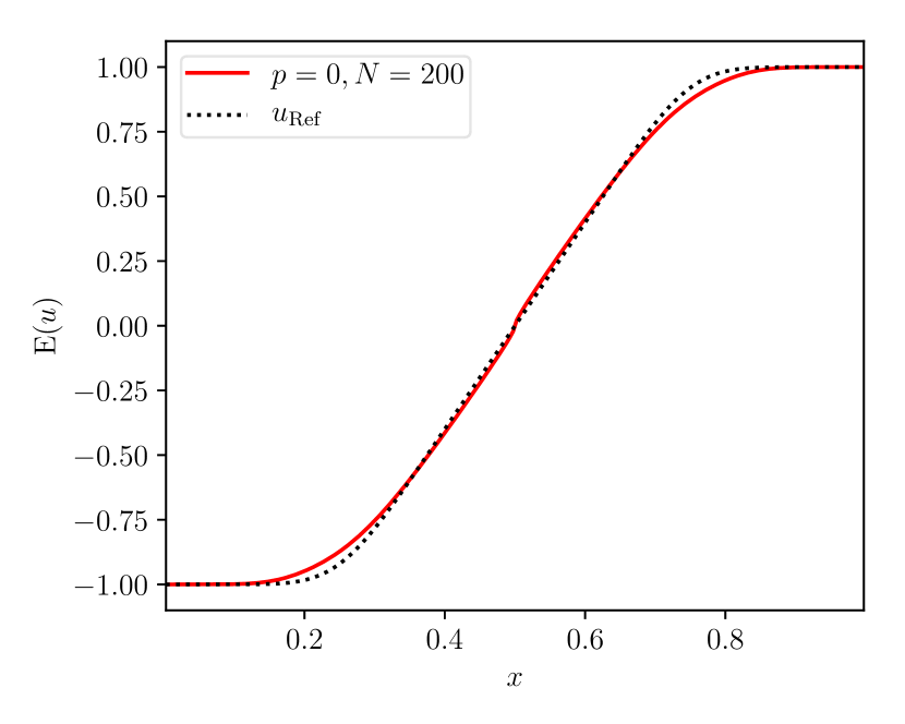
(a) $M=1$, expectation $\operatorname{E}[u]$.

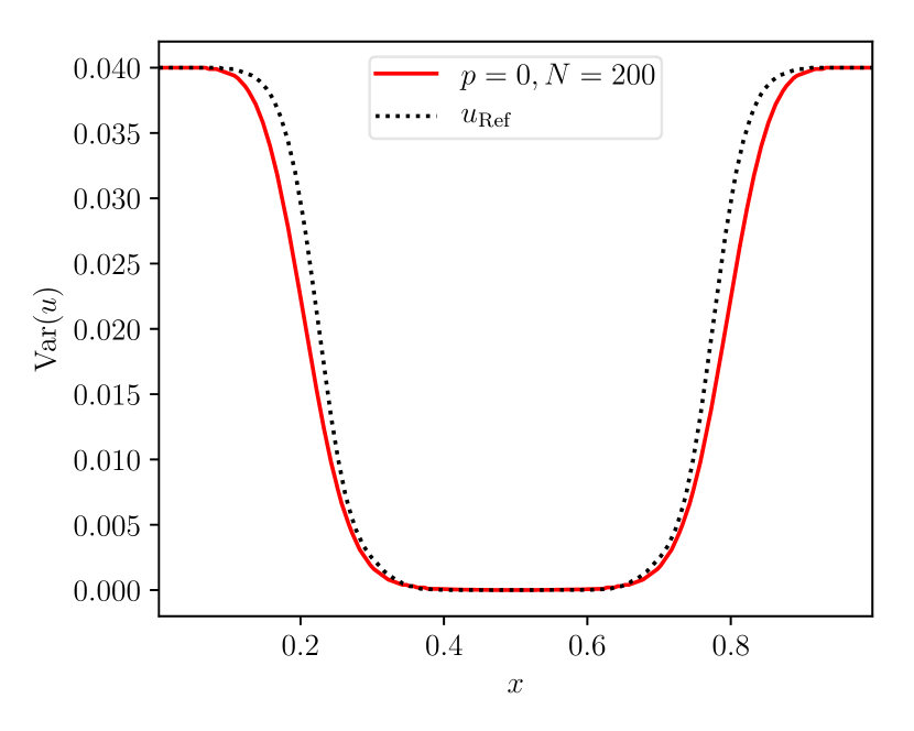
(b) $M=1$, variance $\operatorname{Var}(u)$.

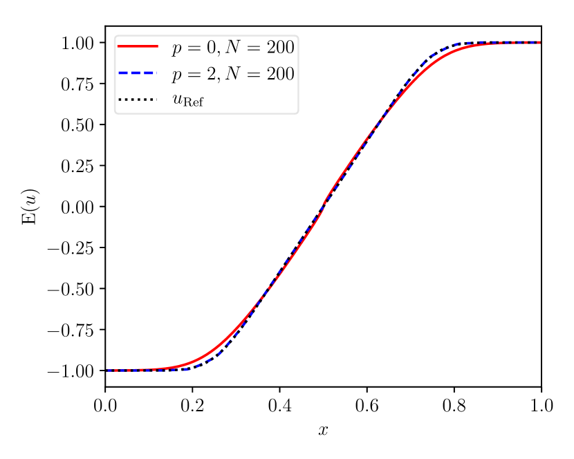
(c) $M=6$, expectation $\operatorname{E}[u]$.

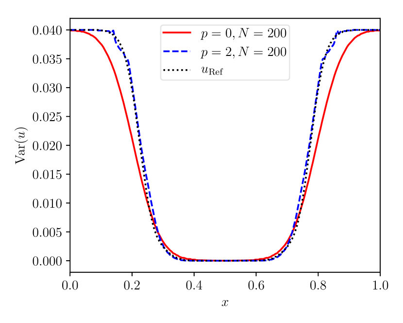
(d) $M=6$, variance $\operatorname{Var}(u)$.

Figure 2: Rarefaction of uncertain height as initial condition for an expansion wave in the solution at time $t=0.25$.

In particular, we note that going from $M=1$ to $M=6$ for $p=0$ and $N=200$ the numerical solution does not improve, see Figure 2(a) compared to Figure 2(c) (expected value) and Figure 2(b) compared to Figure 2(d) (variance). Yet, the numerical solution improves when we simultaneously increase the polynomial degree from $p=0$ to $p=2$.

5.2 Initial Shock

Finally, the stochastic Riemann problem (78) with an initial shock will be covered. Here, the initial condition is

$$u(x,0,\xi(\omega))= \begin{cases}u_{L}=a+p(\xi(\omega))&\text{ if }x<x_{0},\\ u_{R}=-a+p(\xi(\omega))&\text{ if }x>x_{0},\end{cases}$$ (114)

$$u(0,t,\xi(\omega))= \ u_{L},\ u(1,t,\xi(\omega))=u_{R},$$

$$\xi\sim \ \mathcal{N}(0,1),$$

with uncertain strength located at $x_{0}\in[0,1]$ and function $p(\xi(\omega))=b\xi(\omega)$. For the numerical tests, the parameters $a=1$, $b=0.2$ and $x_{0}=0.5$ are considered. As described in section 4.2, Dirichlet boundary conditions are used. This problem has also been treated by Pettersson et al. [28, 27] and thus allows a comparison of the numerical results. Note that the reference solution $u_{\mathrm{Ref}}$ was derived in the previous section 4.2 as the analytical solution of the system (12) of infinite order. For the numerical computations, however, the polynomial chaos expansion is truncated and the system (12) is solved numerically.

Figure 3 displays the expected value $\operatorname{E}[u]$ and the variance $\operatorname{Var}(u)$ of the reference solution and different numerical solutions for $p=0$ at time $t=0.5$. The numerical solutions are computed for $N=100,3200$ and $M=1,2,3$.

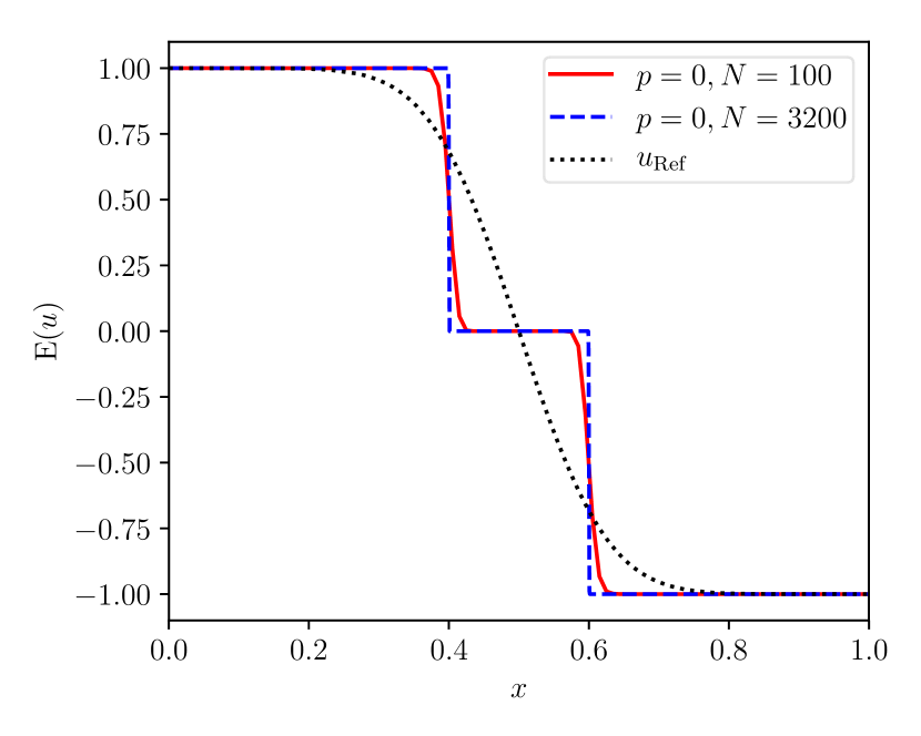
(a) $M=1$, expectation $\operatorname{E}[u]$.

(b) $M=1$, variance $\operatorname{Var}(u)$.

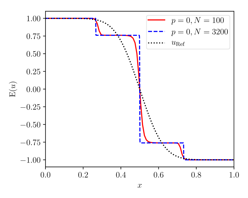
(c) $M=2$, expectation $\operatorname{E}[u]$.

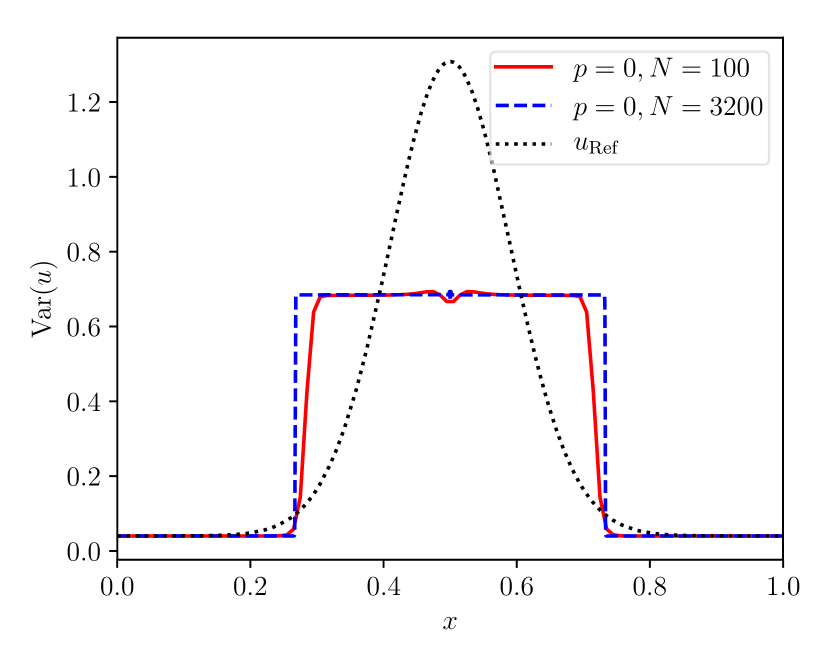
(d) $M=2$, variance $\operatorname{Var}(u)$.

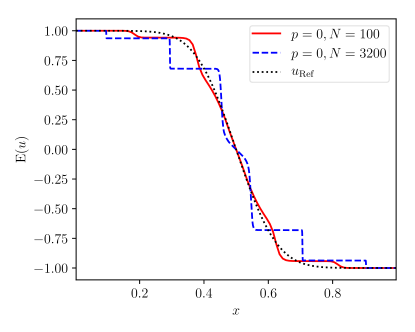
(e) $M=3$, expectation $\operatorname{E}[u]$.

(f) $M=3$, variance $\operatorname{Var}(u)$.

Figure 3: Solution at time $t=0.5$ for a shock of uncertain height as initial condition.

For this test case distinct structures can be observed for the truncated systems of increasing order $M$. While these structures are blurred for the numerical solutions using only $N=100$ elements, they are better resolved for the numerical solution using $N=3200$ elements (compared to a grid convergence study using entropy stable finite volume schemes not presented here in detail). Thus, it should be stressed that an increasing number of elements, i.e. an enhanced spacial resolution, does not result in more accurate numerical solutions compared to the reference solution of the system (12) of infinite order. A similar behaviour was already observed in [28] for this test case: Instead of increasing the polynomial chaos order $M$, one should increase the dissipation that is added to the scheme to smooth the numerical solution. A scheme with a lot of dissipation like the FV scheme with $N=100$ will lead to a solution that appears to be better in comparison with the reference solution for $M\to\infty$. That the dissipation in this test case is very important will also be seen in the following.

Surprisingly, for $M=3$, the numerical solution using $N=100$ elements is not only blurred compared to the more resolved numerical solution using $N=3200$ elements, but displays the jump at different locations. This is illustrated in greater detail in Figure 4, where the numerical solutions for $M=3$, $p=0$, and increasing $N=100,200,400,800,1600,3200$ are shown.

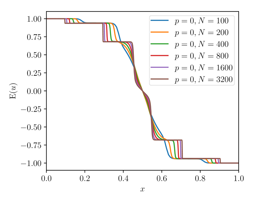
(a) $M=3$, expectation $\operatorname{E}[u]$.

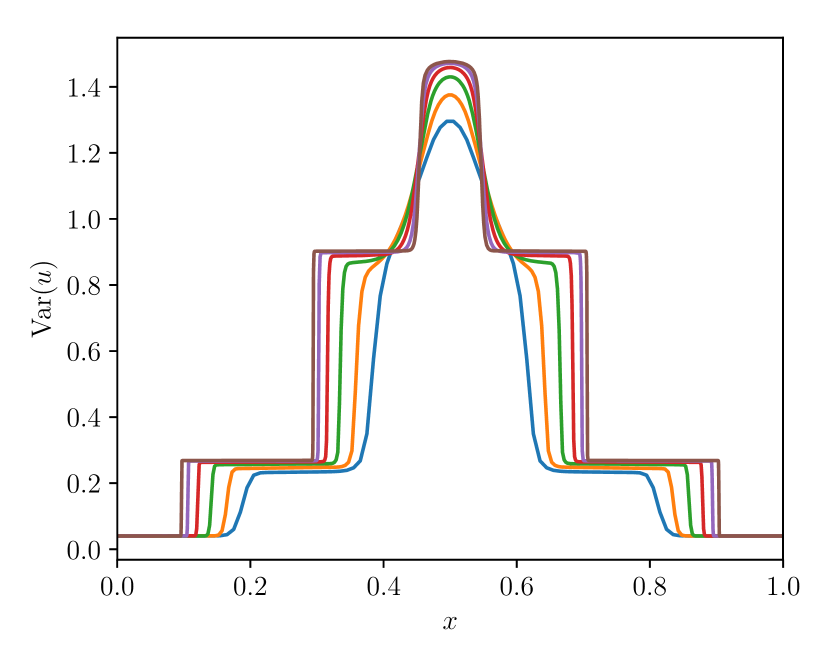
(b) $M=3$, variance $\operatorname{Var}(u)$.

Figure 4: Solution at time $t=0.5$ for a shock of uncertain height as initial condition.

We note that the jump locations are observed to vary with the spacial resolution. A similar behaviour is observed when the polynomial degree $p$ is increased. Then, we get additionally spurious oscillations, resulting from the Gibbs phenomenon. However, a further detail can be observed for the finite order systems. The numerical solution for higher polynomial degrees indicates another structure of the solution. In what follows, this phenomenon is investigated in greater detail.

For $t=0.5$, Figure 5 displays the expectation $\operatorname{E}[u]$ and variance $\operatorname{Var}(u)$ of the numerical solutions from the SBP CPR and FV methods. There, also $\operatorname{E}[u]$ and $\operatorname{Var}(u)$ of the reference solution $u_{\mathrm{Ref}}$ are illustrated. While $N=$2500$$ elements were used for the SBP CPR method with polynomial degree $p=3$, for the corresponding FV methods $N=$10\,000$$ elements were used. In the following for both methods, $100\,000$ time steps were used.

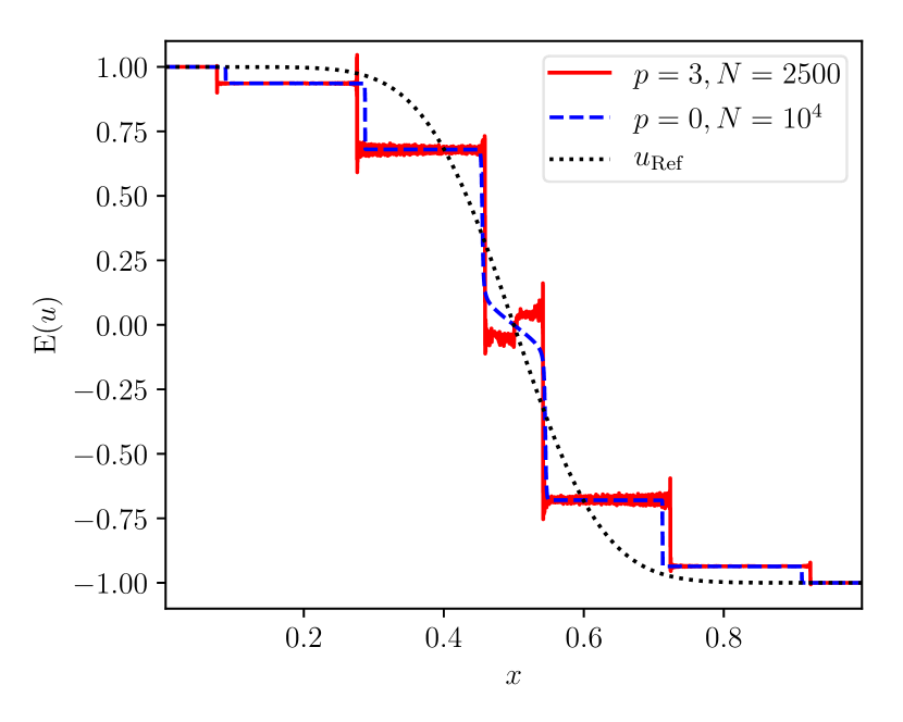
(a) Expectation $\operatorname{E}[u]$.

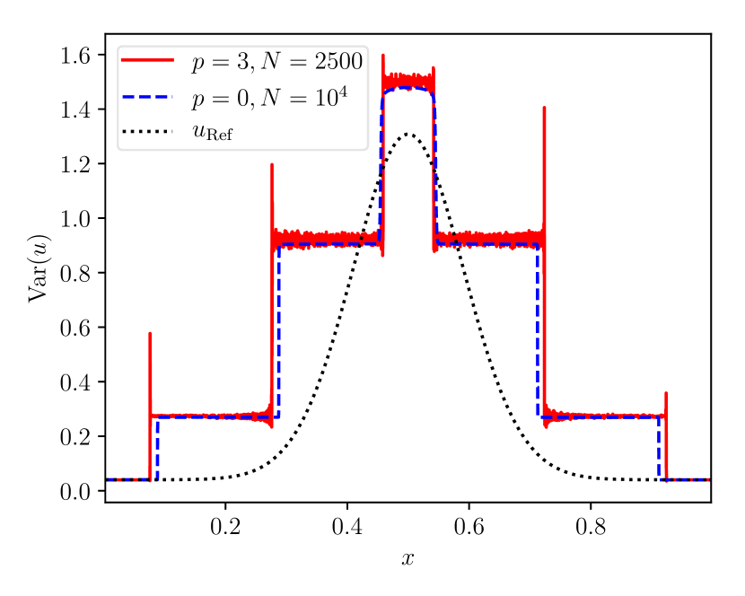
(b) Variance $\operatorname{Var}(u)$.

Figure 5: Solution at time $t=0.5$ for a shock of uncertain height as initial condition.

Three observations should be pointed out immediately:

1. Both numerical solutions differ significantly from the reference solution $u_{\mathrm{Ref}}$.

2. Both numerical solutions show more wave-fronts than one would expect from classical theory of Riemann problems for strictly hyperbolic systems with genuinely nonlinear or linearly degenerate fields.

3. Also the numerical solutions themselves show quite different features, especially in their wave profiles around $x_{0}=0.5$.

The first observation was also pointed out by Pettersson et al. [28, 27] and arises from the truncation of the infinite order system (78) to the four dimensional system (12) for $M=3$. Thus, the analytical solution $u_{\mathrm{Ref}}$ of the infinite order system for $M\to\infty$ differs from ’the analytical solution’ of the truncated system. The latter one is however approximated by the numerical solutions. The difference between $u_{\mathrm{Ref}}$ and the analytical solution to the truncated system already gets stressed by mismatching regularities. While $u_{\mathrm{Ref}}$ was shown to be smooth in the last section, the solution of the truncated system is expected to feature discontinuities. We saw this already before in our numerical tests and refer again to Remark 5.1 and the literature therein.

Naturally the following question arises: What is the analytical solution of the truncated system? For Riemann problems of strictly hyperbolic systems with genuinely nonlinear or linearly degenerate fields, there are in fact clear results in the literature [19] on how solutions behave. In particular, the analytical solution of a $M+1=4$ dimensional system consists of at most $M+2=5$ constant states which are connected by shock discontinuities or expansion waves. At the same time the numerical solutions in Figure 5 both show at least $6$ such constant states. Thus, classical theory of Riemann problems for strictly hyperbolic systems obviously fails. This is due to the assumption of the system to be strictly hyperbolic, i.e. to have real distinct eigenvalues. Already the steady state $(u_{0},u_{1},u_{2},u_{3})=(0,0,0,0)$ yields matrix $A(u)=0$ in (108) to have eigenvalues $\lambda_{1}=\lambda_{2}=\lambda_{3}=\lambda_{4}=0$. Non distinct eigenvalues can also be observed in Figures 7 and 8 for the numerical solutions of this particular Riemann problem.

Remark 5.2.

For scalar conservation laws, the PC approach yields a symmetric system. Due to the symmetry, the arising system is therefore hyperbolic, see [42, 6]. In general, the arising system is however nonstrictly hyperbolic. To calculate the exact analytical solution for this system, the eigenvalues have to be known. Indeed, further results can be found in the literature, e.g. that they are analytical [18, Chapter II, Theorem 1.8]. Nevertheless, without further assumptions on the entries of the $4\times 4$ symmetric matrix, the eigenvalues can not be expressed by a simple and closed formula [private communication with Harald Löwe, TU Braunschweig]. This can be proved by an algebraic approach and it is beyond the scope of this paper.

Finally, the third observation - different profiles of the numerical solutions - shall be addressed. In Figure 5, the numerical solutions for the SBP CPR method and the corresponding FV method essentially differ in three aspects:

1. Their behaviour near the centre $x_{0}=0.5$.

2. The position of the shock discontinuities away from $x_{0}=0.5$, e.g. at $x\approx 0.276$ for the SBP CPR method and at $x\approx 0.287$ for the FV method.

3. The height of the constant states. This can’t be seen without zooming in, which is therefore done in Figure 6.

Noticing these differences, another question arises: What is the mechanism behind this?

By a large number of different tests for the SBP CPR, FV and SBP FD method, the numerical dissipation added by the underlying scheme was explored as the determining factor. As Figure 6 demonstrates, different profiles for the expectation $\operatorname{E}[u]$ can be reproduced by all of the three methods. The plot (a) and (b) show the expectation $\operatorname{E}[u]$ and variance $\operatorname{Var}(u)$ for the SBP CPR method, (c) and (d) for the FV method, and (e) and (f) for the SBP FD method. The (red) solid line thereby illustrates a numerical solution obtained by the corresponding method equipped with low numerical dissipation. The (blue) dashed line, on the other hand, illustrates a numerical solution obtained by the corresponding method equipped with high numerical dissipation.

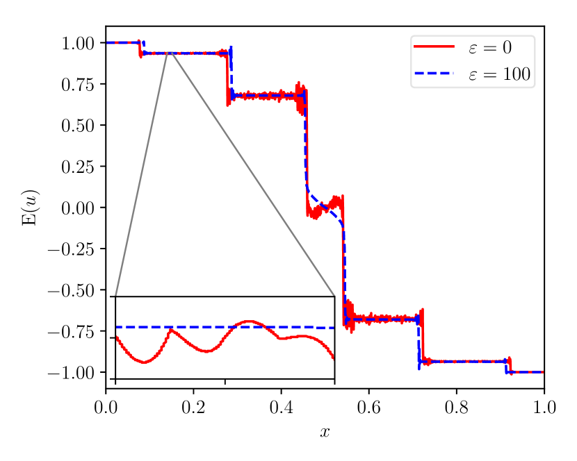
(a) CPR, expectation $\operatorname{E}[u]$.

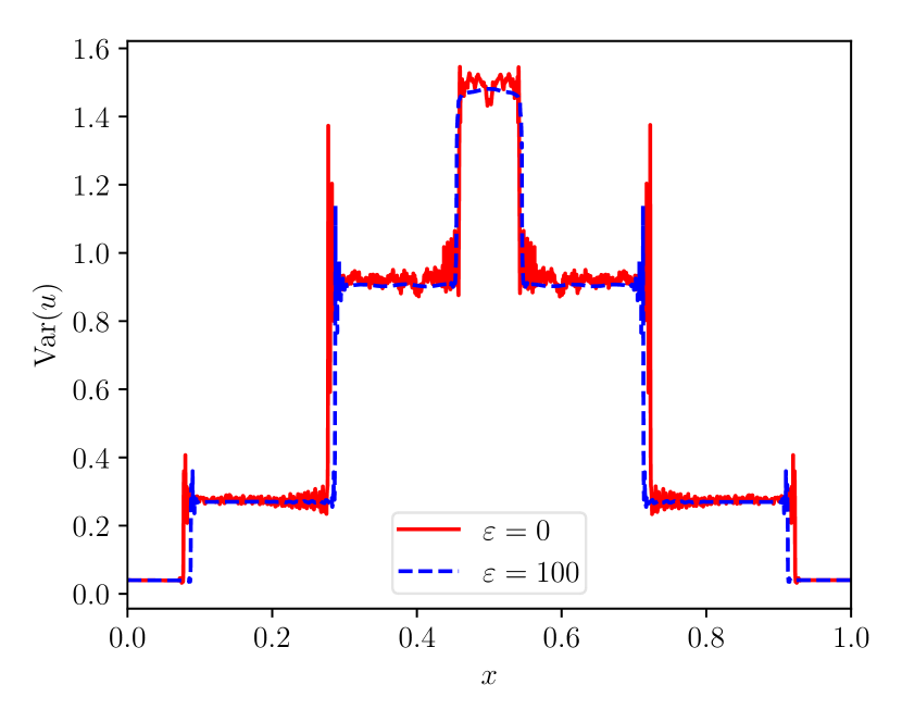
(b) CPR, variance $\operatorname{Var}(u)$.

(c) FV, expectation $\operatorname{E}[u]$.

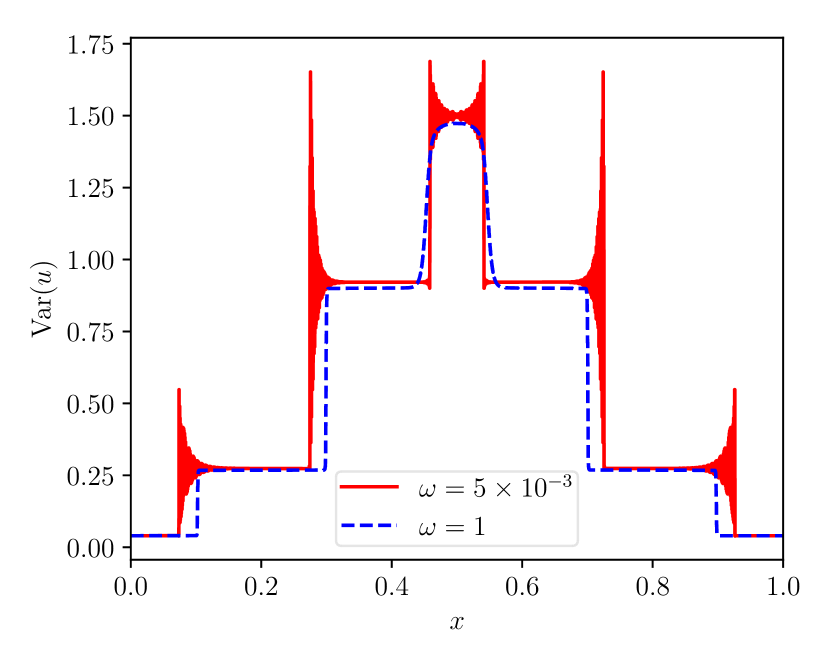
(d) FV, variance $\operatorname{Var}(u)$.

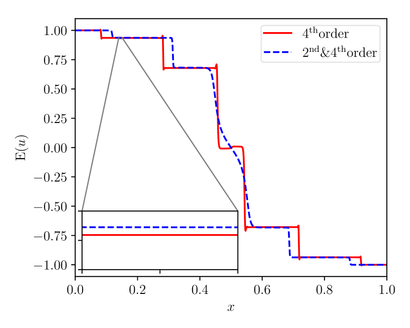
(e) FD, expectation $\operatorname{E}[u]$.

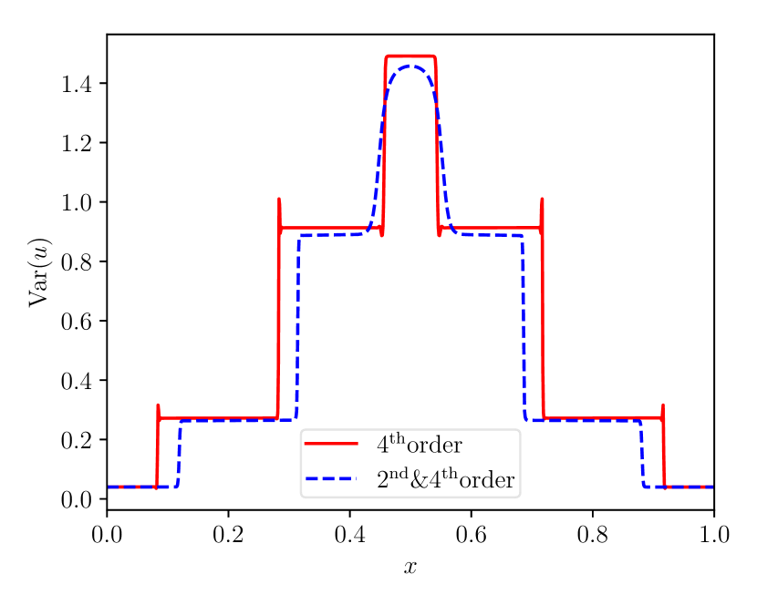
(f) FD, variance $\operatorname{Var}(u)$.

Figure 6: Scaled numerical dissipation for the shock of uncertain height as initial condition. Numerical solutions by SBP CPR, FV and SBP FD. Parameters: Polynomial chaos order $M=3$, final time $t=0.5$, inflow boundary conditions.

In case of the SBP CPR method, numerical dissipation was added by applying modal filtering by an exponential filter of order $s=1$ and strength $\varepsilon=100$ in every element and after every time step. See [31, 13, 14] for details.

For the FV method however, already showing a smeared profile, numerical dissipation was reduced. This was done by multiplying the dissipation matrix added to the entropy conservative flux with decreasing weights $0<\omega\leq 1$.

Numerical dissipation in the SBP FD method of Pettersson et al. [28, 27] refers to artificial dissipation terms of second and fourth order, see [20, 25] for details. Thus, the original conservation law is extended by viscosity terms of second and fourth order derivatives which are properly discretised and weighted. To reduce numerical dissipation, the second order derivative was nullified and just the fourth order derivative was used for the artificial dissipation. The results for the SBP FD method were furthermore computed by the matlab code of Pettersson et al. which they have offered very well prepared in [27].

Summarising the results from the described numerical tests, the following can be observed.

Remark 5.3.

The numerical solutions of the truncated system (114) for $M=3$ differ significantly with respect to the numerical dissipation added by the underlying scheme. In particular, the wave profile near $x_{0}=0.5$ shows quite varying features.
As it is already investigated and summarised in [27, Chapter 6] for SBP FD methods, the influence of dissipation is enormously in the PC approach. Excessive use of artificial dissipation can give a numerical solution that more closely resemble the solution for the original problem ($M\to\infty$) compared to a solution where the order of the polynomial chaos method is increased and only a small amount of dissipation is applied, but these features of the deterministic $4\times 4$ system are not even mentioned there. The numerical solutions may differ significantly depending on the artificial dissipation of the schemes, see for instance [20]. But even with this knowledge, these specifics look impressive. From a heuristic point of view, the numerical solutions calculated with the higher amount of dissipation seem more reasonable after all, but to be sure, one has to analyse it. The impression suggests a contact discontinuity at this point, which yields these different numerical solutions depending on the dissipation.

Since no analytical solution of the observed system is known, other criteria should be examined. The idea is to identify numerical solutions which are physically reasonable and to reject the ones which are not. For solutions of hyperbolic conservation laws to be physically reasonable, typically two conditions are checked. First, the Rankine-Hugoniot jump condition

$$s\!\leavevmode\resizebox{0.0pt}{0.0pt}{ [\![ }\mkern-6.5muu_{k}\mkern-6.5mu\leavevmode\resizebox{0.0pt}{0.0pt}{ ]\!] }\!\!=\!\leavevmode\resizebox{0.0pt}{0.0pt}{ [\![ }\mkern-6.5muf_{k}\mkern-6.5mu\leavevmode\resizebox{0.0pt}{0.0pt}{ ]\!] }\!\!$$ (115)

across every discontinuity, where $s$ is the speed of propagation of the discontinuity. Second, the entropy inequality $\partial_{t}U+\partial_{x}F\leq 0$, which is equivalent to a Rankine-Hugoniot condition for the entropy

$$\!\leavevmode\resizebox{0.0pt}{0.0pt}{ [\![ }\mkern-6.5muF\mkern-6.5mu\leavevmode\resizebox{0.0pt}{0.0pt}{ ]\!] }\!\!\leq s\!\leavevmode\resizebox{0.0pt}{0.0pt}{ [\![ }\mkern-6.5muU\mkern-6.5mu\leavevmode\resizebox{0.0pt}{0.0pt}{ ]\!] }\!\!.$$ (116)

The left hand sides (a) of Figures 7 and 8 each show results from the corresponding method using more dissipation. The results on the right hand sides (b) each show results from the same method using significant less numerical dissipation.

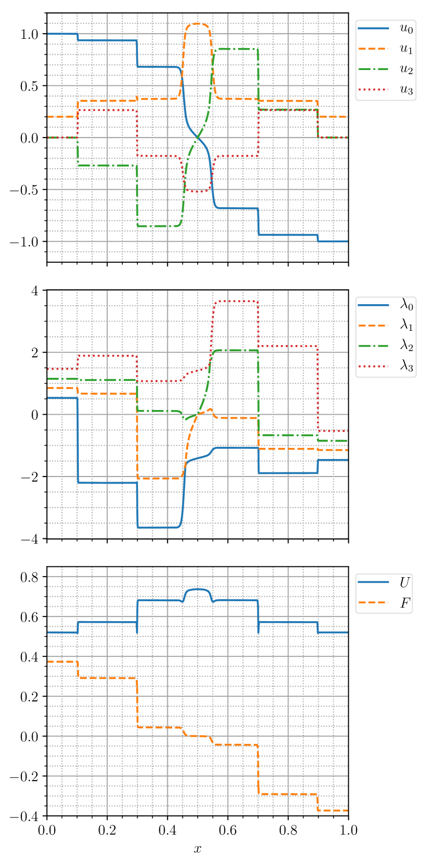
(a) $\omega=1$.

(b) $\omega=5\times 10^{-3}$.

Figure 7: Numerical solutions, eigenvalues, entropy and entropy flux for scaled numerical dissipation for the shock of uncertain height as initial condition. Numerical solutions by FV with ’full’ dissipation $\omega=1$ and reduced dissipation $\omega=5\times 10^{-3}$. Parameters: Polynomial chaos order $M=3$, time boundary $t=0.5$, inflow boundary conditions.

The FV solution in Figure 7 already contains quite spurious oscillations (and the CPR solution even more). Similar plots are given in Figure 8 for the FD solution. These plots show nearly no oscillations.

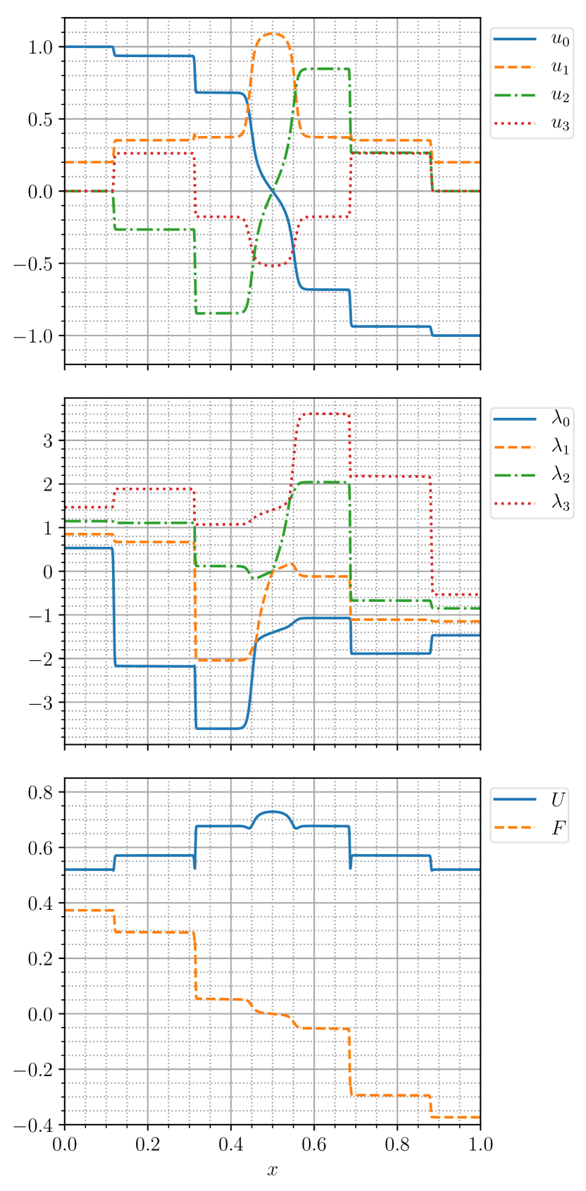
(a) $2^{\mathrm{nd}}$ & $4^{\mathrm{th}}$ order dissipation.

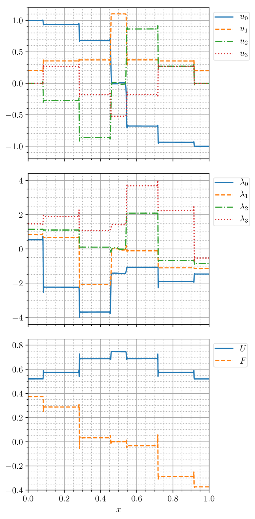
(b) $4^{\mathrm{th}}$ order dissipation.

Figure 8: Numerical solutions, eigenvalues, entropy and entropy flux for scaled numerical dissipation for the shock of uncertain height as initial condition. Numerical solutions by SBP FD with ’full’ dissipation by both, the $2^{\mathrm{th}}$ and $4^{\mathrm{th}}$ order dissipation, and reduced dissipation just by the $4^{\mathrm{th}}$ order dissipation. Parameters: Polynomial chaos order $M=3$, time boundary $t=0.5$, inflow boundary conditions.

Since the essential differences arise near the centre $x_{0}=0.5$, the focus is on the profiles of the numerical solutions there. Both methods lead to smooth non-constant transitions at $x_{0}=0.5$ for high numerical dissipation, see (a) in Figures 7 and 8. At the same time, there is a nearly constant transition for the FD solution with low dissipation, see (b) in Figure 8, and a piecewise constant transition with a up-jump at $x_{0}=0.5$ for the FV solution with even lower numerical dissipation, see (b) in Figure 7.

Except for the last case, the Rankine-Hugoniot jump condition is obviously fulfilled, since no discontinuity occurs. The FV solution (b) in Figure 7 also fulfils this condition with speed of propagation $s=0$.

Furthermore, also the Rankine-Hugoniot jump condition for the entropy (116) is obviously satisfied by all solutions due to no jumps in the entropy $U$ and flux $F$ at $x_{0}=0.5$.

Both approaches do not answer the question of what the physically relevant solution for this system is. Other investigations are necessary.

6 Summary and Conclusions

In this work, a polynomial chaos approach for Burgers’ equation has been applied and the resulting hyperbolic system has been considered in the general framework of CPR methods using SBP operators. Besides conservation, focus was especially given to stability, which was proven for the CPR method and all systems arising from the PC approach. Due to the usage of split-forms similar to [7, 5, 4], the major challenge was to construct entropy stable numerical fluxes. For the first time, this was done rigorously for all systems resulting from the PC approach for Burgers’ equation.

Furthermore, numerical results for two different test cases have been examined. Burgers’ equation with an initial rarefaction demonstrated convergence for the truncated system, whereas for the convergence study to the reference solution a diagonal limit should be used. More interesting, they also highlighted clear differences in numerical dissipation added by the schemes. It became clear in the last test case that this is crucial. In fact, the last test case, i.e. Burgers’ equation with an initial shock, has been the most remarkable one. Quite fascinating observations have been highlighted.

All numerical solutions showed more wave fronts than one would expect from classical theory of Riemann problems for strictly hyperbolic systems with genuinely nonlinear or linearly degenerate fields. Furthermore, the numerical solutions featured quite different behaviours, especially in their wave profiles around $x_{0}=0.5$, highly depending on the numerical dissipation. It seems likely that the numerical schemes with a lot of artificial dissipation yields the correct numerical solutions, but it is still not clear and must further be examined.

In fact, it remains an open problem for nonstrictly hyperbolic systems of conservation laws what (entropy) conditions might ensure uniqueness and even existence of solutions. All of them, just one, or none of the numerical solutions might indeed converge to a reasonable solution. Nevertheless, a quite fascinating dependence on the added numerical dissipation could be observed.

At this point, a broad field of open problems for the analytical as well as numerical treatment of (nonstrictly) hyperbolic problems arises. In particular, the authors look forward to further research on this.

Appendix A Appendix

A.1 Hermite Polynomials

The probabilistic version of the Hermite polynomials has as weight function $\varrho(y)=\frac{1}{\sqrt{2\pi}}\exp{\frac{-y^{2}}{2}}$. This is the probability density function of a Gaussian distribution. Therefore, using normalised Hermite polynomials as basis functions is an intuitive choice. A table of the “natural” orthogonal basis functions in dependence of different distributions of random variables is given in [43, Table 4.1]. Here, we restrict ourselves to Gaussian measures and so we will only repeat the main properties of the normalised Hermite polynomials. These and further results can be found in [2, 36].

The inner product of the normalised Hermite polynomials $\varphi$ of a Gaussian variable $\xi$ is defined by

$$\operatorname{E}[\varphi_{i}\varphi_{j}]=\int_{\mathbb{R}}\varphi_{i}(y)\varphi_{j}(y)\varrho(y)\operatorname{d\!}y=\delta_{i,j}.$$ (117)

The triple product is given by

$$\operatorname{E}[\varphi_{i}\varphi_{j}\varphi_{k}]=\begin{cases}0\qquad&\text{ if $i+j+k$ is odd or $\max(i,j,k)>s$ },\\ \frac{\sqrt{i!j!k!}}{(s-i)!(s-j)!(s-k)!}\qquad&\text{ otherwise},\end{cases}$$ (118)

where $s=(i+j+k)/2$.

We also need the following relation

$$\sqrt{i}\varphi_{i}\varrho=-\left(\varphi_{i-1}\varrho\right)^{\prime}.$$ (119)

A.2 Stability of CPR Method

Here, we present the calculation for equation (32) from subsection 3.2 in detail. This is similar to the work of [28]. We start with (29) and consider

$$\partial_{t}\underline{u}+\frac{\beta}{2}(\underline{\underline{D}}\,\otimes\hat{\operatorname{I}})A_{G}\underline{u}+(1-\beta)\left(A_{G}(\underline{\underline{D}}\,\otimes\hat{\operatorname{I}})\underline{u}\right)+\left(\left(\underline{\underline{M}}{{}^{-1}}\underline{\underline{R}}{{}^{T}}\underline{\underline{B}}\,\right)\otimes\hat{\operatorname{I}}\right)\left(\underline{f}^{\mathrm{num}}-\frac{1}{2}(\underline{\underline{R}}\,\otimes\hat{\operatorname{I}})A_{G}\underline{u}\right) =0,$$ (120)

where $\underline{f}^{\mathrm{num}}$ is the numerical flux and $\underline{u}=\left(u_{0}(\zeta_{0}),\dots,u_{0}(\zeta_{p}),u_{1}(\zeta_{0}),\dots,u_{M}(\zeta_{p})\right)^{T}$ is the combination vector from SBP CPR and the polynomial chaos method. Investigating $\mathbf{L}^{2}$ stability, we multiply (29) with $\underline{u}^{T}(\underline{\underline{M}}\,\otimes\hat{\operatorname{I}})$. With the SBP property (20), we get

$$\frac{1}{2}\frac{\operatorname{d\!}}{\operatorname{d\!}t}\mathinner{\!\left\lVert\underline{u}\right\rVert}_{\underline{\underline{M}}\,\otimes\hat{\operatorname{I}}}^{2}=\underline{u}^{T}(\underline{\underline{M}}\,\otimes\hat{\operatorname{I}})(\hat{\operatorname{I}}\otimes\underline{\underline{\operatorname{I}}}\,)\partial_{t}\underline{u}$$ (121)

$$= -\frac{\beta}{2}\underline{u}^{T}(\underline{\underline{M}}\,\otimes\hat{\operatorname{I}})(\underline{\underline{D}}\,\otimes\hat{\operatorname{I}})A_{G}\underline{u}-(1-\beta)\underline{u}^{T}(\underline{\underline{M}}\,\otimes\hat{\operatorname{I}})A_{G}(\underline{\underline{D}}\,\otimes\hat{\operatorname{I}})\underline{u}$$

$$-\underline{u}^{T}(\underline{\underline{M}}\,\underline{\underline{M}}{{}^{-1}}\underline{\underline{R}}{{}^{T}}\underline{\underline{B}}\,\otimes\hat{\operatorname{I}})\left(\underline{f}^{\mathrm{num}}-\frac{1}{2}(\underline{\underline{R}}\,\otimes\hat{\operatorname{I}})A_{G}\underline{u})\right)$$

$$= -\frac{\beta}{2}\underline{u}^{T}(\underline{\underline{M}}\,\underline{\underline{D}}\,\otimes\hat{\operatorname{I}})A_{G}\underline{u}-(1-\beta)\underline{u}^{T}(\underline{\underline{M}}\,\otimes\hat{\operatorname{I}})A_{G}(\underline{\underline{D}}\,\otimes\hat{\operatorname{I}})\underline{u}-\underline{u}^{T}(\underline{\underline{R}}\,^{T}\underline{\underline{B}}\,\otimes\hat{\operatorname{I}})\left(\underline{f}^{\mathrm{num}}-\frac{1}{2}(\underline{\underline{R}}\,\otimes\hat{\operatorname{I}})A_{G}\underline{u}\right)$$

$$= \frac{\beta}{2}\underline{u}^{T}(\underline{\underline{D}}\,^{T}\underline{\underline{M}}\,\otimes\hat{\operatorname{I}})A_{G}\underline{u}-\frac{\beta}{2}\underline{u}^{T}(\underline{\underline{R}}\,^{T}\underline{\underline{B}}\,\underline{\underline{R}}\,\otimes\hat{\operatorname{I}})A_{G}\underline{u}-(1-\beta)\underline{u}^{T}(\underline{\underline{M}}\,\otimes\hat{\operatorname{I}})A_{G}(\underline{\underline{D}}\,\otimes\hat{\operatorname{I}})A_{G}(\underline{\underline{D}}\,\otimes\hat{\operatorname{I}})\underline{u}$$

$$-\underline{u}^{T}(\underline{\underline{R}}\,^{T}\underline{\underline{B}}\,\otimes\hat{\operatorname{I}})\left(\underline{f}^{\mathrm{num}}-\frac{1}{2}(\underline{\underline{R}}\,\otimes\hat{\operatorname{I}})A_{G}\underline{u}\right).$$

We choose $\beta=\frac{2}{3}$. This yields

$$\frac{1}{2}\frac{\operatorname{d\!}}{\operatorname{d\!}t}\mathinner{\!\left\lVert u\right\rVert}_{M\otimes\hat{\operatorname{I}}}^{2}= \frac{1}{3}\underline{u}^{T}(\underline{\underline{D}}\,^{T}\otimes\hat{\operatorname{I}})(\underline{\underline{M}}\,\otimes\hat{\operatorname{I}})A_{G}\underline{u}-\frac{1}{3}\underline{u}^{T}(\underline{\underline{R}}\,^{T}\underline{\underline{B}}\,\underline{\underline{R}}\,\otimes\hat{\operatorname{I}})A_{G}\underline{u}$$ (122)

$$-\frac{1}{3}\underline{u}^{T}(\underline{\underline{M}}\,\otimes\hat{\operatorname{I}})A_{G}(\underline{\underline{D}}\,\otimes\hat{\operatorname{I}})A_{G}(\underline{\underline{D}}\,\otimes\hat{\operatorname{I}})\underline{u}-\underline{u}^{T}(\underline{\underline{R}}\,^{T}\underline{\underline{B}}\,\otimes\hat{\operatorname{I}})\left(\underline{f}^{\mathrm{num}}-\frac{1}{2}(\underline{\underline{R}}\,\otimes\hat{\operatorname{I}})A_{G}\underline{u}\right).$$

$A_{G}$ commutes with $\underline{\underline{M}}\,\otimes\hat{\operatorname{I}}$. This means that

$$A_{G}=(\underline{\underline{M}}\,\otimes\hat{\operatorname{I}})A_{G}(\underline{\underline{M}}\,^{-1}\otimes\hat{\operatorname{I}}).$$ (123)

Applying this fact, we get

$$\frac{1}{3}\underline{u}^{T}(\underline{\underline{D}}\,^{T}\otimes\hat{\operatorname{I}})(\underline{\underline{M}}\,\otimes\hat{\operatorname{I}})A_{G}u =\frac{1}{2}\left((\underline{\underline{D}}\,\otimes\hat{\operatorname{I}})\underline{u}\right)^{T}(\underline{\underline{M}}\,\otimes\hat{\operatorname{I}})A_{G}\underline{u}=\frac{1}{3}\left[(A_{G}u)^{T}(\underline{\underline{M}}\,\otimes\hat{\operatorname{I}})^{T}(\underline{\underline{D}}\,\otimes\hat{\operatorname{I}})\underline{u})\right]^{T}$$ (124)

$$=\frac{1}{3}\underline{u}^{T}(\underline{\underline{M}}\,\otimes\hat{\operatorname{I}})A_{G}(\underline{D}\otimes\hat{\operatorname{I}})\underline{u}.$$

Finally, we employ this in (122) and receive

$$\frac{1}{2}\frac{\operatorname{d\!}}{\operatorname{d\!}t}\mathinner{\!\left\lVert u\right\rVert}_{\underline{\underline{M}}\,\otimes\hat{\operatorname{I}}}^{2}=\frac{1}{6}\underline{u}^{T}(\underline{\underline{R}}\,^{T}\underline{\underline{B}}\,\underline{\underline{R}}\,\otimes\hat{\operatorname{I}})A_{G}\underline{u}-\underline{u}^{T}(\underline{\underline{R}}\,^{T}\underline{\underline{B}}\,\otimes\hat{\operatorname{I}})\underline{f}^{\mathrm{num}}.$$ (125)

Inserting the right and left values in one element, we get we get

$$\frac{1}{2}\frac{\operatorname{d\!}}{\operatorname{d\!}t}\mathinner{\!\left\lVert u\right\rVert}^{2}_{\underline{\underline{M}}\,\otimes\hat{\operatorname{I}}}=\frac{1}{6}u^{(e),T}_{R}A(u^{(e)}_{R})u^{(e)}_{R}-\frac{1}{6}u^{(e),T}_{L}A(u^{(e)}_{L})u^{(e)}_{L}+u^{(e),T}_{L}f^{\mathrm{num},e}_{L}-u^{(e),T}_{R}f^{\mathrm{num},e}_{R}.$$ (30)

References

• [1] R. Abgrall and S. Mishra. Uncertainty quantification for hyperbolic systems of conservation laws. In Handbook of Numerical Analysis, volume 18, pages 507–544. Elsevier, 2017.
• [2] M. Abramowitz and I. A. Stegun. Handbook of mathematical functions. National Bureau of Standards, 1972.
• [3] R. H. Cameron and W. T. Martin. The orthogonal development of non-linear functionals in series of Fourier-Hermite functionals. Annals of Mathematics, pages 385–392, 1947.
• [4] M. H. Carpenter and T. C. Fisher. High-order entropy stable formulations for computational fluid dynamics. In 21st AIAA Computational Fluid Dynamics Conference. American Institute of Aeronautics and Astronautics, 2013.
• [5] M. H. Carpenter, T. C. Fisher, E. J. Nielsen, and S. H. Frankel. Entropy stable spectral collocation schemes for the Navier-Stokes equations: Discontinuous interfaces. SIAM Journal on Scientific Computing, 36(5):B835–B867, 2014.
• [6] A. Chertock, S. Jin, and A. Kurganov. An operator splitting based stochastic Galerkin method for the one-dimensional compressible Euler equations with uncertainty, 2015. http://www.ki-net.umd.edu/pubs/files/Euler-UQ.pdf.
• [7] T. C. Fisher and M. H. Carpenter. High-order entropy stable finite difference schemes for nonlinear conservation laws: Finite domains. Journal of Computational Physics, 252:518–557, 2013.
• [8] T. C. Fisher, M. H. Carpenter, J. Nordström, N. K. Yamaleev, and C. Swanson. Discretely conservative finite-difference formulations for nonlinear conservation laws in split form: Theory and boundary conditions. Journal of Computational Physics, 234:353–375, 2013.
• [9] G. J. Gassner. A skew-symmetric discontinuous Galerkin spectral element discretization and its relation to SBP-SAT finite difference methods. SIAM Journal on Scientific Computing, 35(3):A1233–A1253, 2013.
• [10] G. J. Gassner, A. R. Winters, and D. A. Kopriva. Split form nodal discontinuous Galerkin schemes with summation-by-parts property for the compressible Euler equations. Journal of Computational Physics, 327:39–66, 2016.
• [11] R. G. Ghanem and P. D. Spanos. Stochastic finite elements: a spectral approach. Courier Corporation, 2003.
• [12] J. Giesselmann, F. Meyer, and C. Rohde. A posteriori error analysis for random scalar conservation laws using the stochastic galerkin method. arXiv preprint arXiv:1709.04351, 2017.
• [13] J. Glaubitz, P. Öffner, H. Ranocha, and T. Sonar. Artificial viscosity for correction procedure via reconstruction using summation-by-parts operators. In XVI International Conference on Hyperbolic Problems: Theory, Numerics, Applications, pages 363–375. Springer, 2016.
• [14] J. Glaubitz, P. Öffner, and T. Sonar. Application of modal filtering to a spectral difference method. Mathematics of Computation, 87(309):175–207, 2018.
• [15] S. Gottlieb and C.-W. Shu. Total variation diminishing Runge-Kutta schemes. Mathematics of Computation, 67(221):73–85, 1998.
• [16] H. Huynh. A flux reconstruction approach to high-order schemes including discontinuous Galerkin methods. AIAA paper, 4079:2007, 2007.
• [17] H. Huynh, Z. J. Wang, and P. E. Vincent. High-order methods for computational fluid dynamics: A brief review of compact differential formulations on unstructured grids. Computers & Fluids, 98:209–220, 2014.
• [18] T. Kato. Perturbation Theory for Linear Operators. Springer-Verlag Berlin Heidelberg, 1995.
• [19] P. D. Lax. Hyperbolic systems of conservation laws and the mathematical theory of shock waves. SIAM, 1973.
• [20] K. Mattsson, M. Svärd, and J. Nordström. Stable and accurate artificial dissipation. Journal of Scientific Computing, 21(1):57–79, 2004.
• [21] F. Meyer, L. Schlachter, and F. Schneider. A hyperbolicity-preserving discontinuous stochastic Galerkin scheme for uncertain hyperbolic systems of equations. ArXiv e-prints, May 2018. arXiv:1805.10177.
• [22] S. Mishra, N. H. Risebro, C. Schwab, and S. Tokareva. Numerical solution of scalar conservation laws with random flux functions. SIAM/ASA Journal on Uncertainty Quantification, 4(1):552–591, 2016.
• [23] S. Mishra and C. Schwab. Sparse tensor multi-level monte carlo finite volume methods for hyperbolic conservation laws with random initial data. Mathematics of Computation, 81(280):1979–2018, 2012.
• [24] S. Mishra, C. Schwab, and J. Šukys. Multi-level monte carlo finite volume methods for uncertainty quantification in nonlinear systems of balance laws. In Uncertainty quantification in computational fluid dynamics, pages 225–294. Springer, 2013.
• [25] J. Nordström. Conservative finite difference formulations, variable coefficients, energy estimates and artificial dissipation. Journal of Scientific Computing, 29(3):375–404, 2006.
• [26] J. Nordström. A roadmap to well posed and stable problems in computational physics. Journal of Scientific Computing, 71(1):365–385, 2017.
• [27] M. P. Pettersson, G. Iaccarino, and J. Nordström. Polynomial Chaos Methods for Hyperbolic Partial Differential Equations: Numerical Techniques for Fluid Dynamics Problems in the Presence of Uncertainties. Springer, 2015.
• [28] P. Pettersson, G. Iaccarino, and J. Nordström. Numerical analysis of the Burgers’ equation in the presence of uncertainty. Journal of Computational Physics, 228(22):8394–8412, 2009.
• [29] G. Poëtte, B. Després, and D. Lucor. Uncertainty quantification for systems of conservation laws. Journal of Computational Physics, 228(7):2443–2467, 2009.
• [30] H. Ranocha. Shallow water equations: Split-form, entropy stable, well-balanced, and positivity preserving numerical methods. GEM – International Journal on Geomathematics, 8(1):85–133, 04 2017. arXiv:1609.08029.
• [31] H. Ranocha, J. Glaubitz, P. Öffner, and T. Sonar. Stability of artificial dissipation and modal filtering for flux reconstruction schemes using summation-by-parts operators. Applied Numerical Mathematics, 128:1–23, 2018.
• [32] H. Ranocha and P. Öffner. $L_{2}$ stability of explicit Runge-Kutta schemes. Journal of Scientific Computing, 75(2):1040–1056, 2018.
• [33] H. Ranocha, P. Öffner, and T. Sonar. Summation-by-parts operators for correction procedure via reconstruction. Journal of Computational Physics, 311:299–328, 2016. arXiv:1511.02052.
• [34] H. Ranocha, P. Öffner, and T. Sonar. Extended skew-symmetric form for summation-by-parts operators and varying Jacobians. Journal of Computational Physics, 342:13–28, 04 2017. arXiv:1511.08408.
• [35] M. Svärd and J. Nordström. Review of summation-by-parts schemes for initial-boundary-value problems. Journal of Computational Physics, 268:17–38, 2014.
• [36] G. Szegö. Orthogonal Polynomials, volume 23 of Colloquium Publications. American Mathematical Society, Providence, Rhode Island, 1975.
• [37] E. Tadmor. The numerical viscosity of entropy stable schemes for systems of conservation laws. I. Mathematics of Computation, 49(179):91–103, 1987.
• [38] E. Tadmor. From semidiscrete to fully discrete: Stability of Runge-Kutta schemes by the energy method. ll. Collected lectures on the preservation of stability under discretization, 109:25, 2002.
• [39] E. Tadmor. Entropy stability theory for difference approximations of nonlinear conservation laws and related time-dependent problems. Acta Numerica, 12:451–512, 2003.
• [40] Z. Wang and H. Gao. A unifying lifting collocation penalty formulation including the discontinuous Galerkin, spectral volume/difference methods for conservation laws on mixed grids. Journal of Computational Physics, 228(21):8161–8186, 2009.
• [41] N. Wiener. The homogeneous chaos. American Journal of Mathematics, 60(4):897–936, 1938.
• [42] D. Xiu. Numerical methods for stochastic computations: a spectral method approach. Princeton University Press, 2010.
• [43] D. Xiu and G. E. Karniadakis. The Wiener–Askey polynomial chaos for stochastic differential equations. SIAM Journal on Scientific Computing, 24(2):619–644, 2002.
• [44] D. Xiu and G. E. Karniadakis. Modeling uncertainty in flow simulations via generalized polynomial chaos. Journal of Computational Physics, 187(1):137–167, 2003.
• [45] D. Xiu and G. E. Karniadakis. Supersensitivity due to uncertain boundary conditions. International Journal for Numerical Methods in Engineering, 61(12):2114–2138, 2004.