Elucidating fluctuating diffusivity in center-of-mass motion of
polymer models with time-averaged mean-square-displacement tensor

Abstract

There have been increasing reports that the diffusion coefficient of macromolecules depends on time and fluctuates randomly. Here a novel method is developed to elucidate this fluctuating diffusivity from trajectory data. The time-averaged mean square displacement (MSD), a common tool in single-particle-tracking (SPT) experiments, is generalized to a second-order tensor, with which both magnitude and orientation fluctuations of the diffusivity can be clearly detected. This new method is used to analyze the center-of-mass motion of four fundamental polymer models: the Rouse model, the Zimm model, a reptation model, and a rigid rod-like polymer. It is found that these models exhibit distinctly different types of magnitude and orientation fluctuations of the diffusivity. This is an advantage of the present method over previous ones such as the ergodicity-breaking parameter and a non-Gaussian parameter, because with either of these parameters it is difficult to distinguish the dynamics of the four polymer models. Also, the present method of a time-averaged MSD tensor could be used to analyze trajectory data obtained in SPT experiments.

I Introduction

Macromolecular diffusion in cytoplasm and cell membranes has received much attention in recent years, because it controls chemical kinetics and information processing in cells Berg et al. (1981). Single-particle-tracking (SPT) techniques have been used to study macromolecular diffusion in living systems, and remarkably complicated phenomena such as anomalous diffusion, weak ergodicity breaking (EB), and sample-to-sample fluctuations of the diffusion coefficient have been reported Golding and Cox (2006); Weigel et al. (2011); Parry et al. (2014); Jeon et al. (2011); Tabei et al. (2013). In such SPT experiments, a time average is commonly used to obtain the mean square displacement (MSD); the time-averaged MSD (TMSD) of a tagged particle is defined by Nordlund (1914); He et al. (2008); Metzler et al. (2014)

$$\overline{\delta\bm{r}^{2}}(\Delta,t):=\frac{1}{t-\Delta}\int_{0}^{t-\Delta}\delta\bm{r}^{2}(\Delta,t^{\prime})\,dt^{\prime},$$ (1)

where $\Delta$ is a lag time and $t$ is the total measurement time. In addition, a displacement vector $\delta\bm{r}(\Delta,t^{\prime})$ is defined as $\delta\bm{r}(\Delta,t^{\prime}):=\bm{r}(t^{\prime}+\Delta)-\bm{r}(t^{\prime}),$ where $\bm{r}(t^{\prime})$ is the position vector of the tagged particle at time $t^{\prime}$. Thus, the TMSD $\overline{\delta\bm{r}^{2}}(\Delta,t)$ can be obtained from a single trajectory $\bm{r}(t^{\prime})$.

In SPT experiments of macromolecules in living systems, sample-to-sample fluctuations of the diffusion coefficient have been observed frequently Golding and Cox (2006); Weigel et al. (2011); Parry et al. (2014); Jeon et al. (2011); Tabei et al. (2013). As stated above, the TMSD curve $\overline{\delta\bm{r}^{2}}(\Delta,t)$ (as a function of $\Delta$) is obtained from a single trajectory $\bm{r}(t^{\prime})$, and then, from this TMSD curve, the diffusion coefficient for that trajectory can be estimated. The values of this diffusion coefficient vary from trajectory to trajectory, but, for long trajectories (namely, at $t\to\infty$), they converge to a single value if the system is ergodic. In some SPT experiments, however, the values of the diffusion coefficient are scattered even for long trajectories, and this phenomenon cannot be explained by the ordinary Brownian motion Golding and Cox (2006); Jeon et al. (2011); Weigel et al. (2011); Tabei et al. (2013); Parry et al. (2014).

To explain such sample-to-sample fluctuation in the diffusivity, much effort has been devoted to investigating simple theoretical models such as the continuous-time random walk (CTRW) He et al. (2008); Lubelski et al. (2008); Neusius et al. (2009); Miyaguchi and Akimoto (2011, 2013); Thiel and Sokolov (2014a), fractional Brownian motion Deng and Barkai (2009); Thiel and Sokolov (2014b), and the random walk on fractals Miyaguchi and Akimoto (2015); Meroz et al. (2010). In these studies, the variance of the TMSD, which is commonly referred to as the EB parameter, has been used to characterize the fluctuation in the diffusivity. In particular, it was shown that the EB parameter for the CTRW converges to a non-vanishing value as $t\to\infty$. In other words, the TMSD behaves as a random variable even for long measurement times. Therefore, CTRW-like dynamics have been considered to be a factor in the sample-to-sample fluctuation of the diffusivity observed in SPT experiments He et al. (2008); Lubelski et al. (2008); Neusius et al. (2009).

However, fluctuations in diffusivity originate also from correlated dynamics of inner degrees of freedom. In Ref. Uneyama et al. (2015), the authors studied a reptation model (a tagged polymer model in entangled polymer solutions) and showed that the EB parameter of the center-of-mass (COM) motion is non-vanishing for quite a long measurement time. In other words, the system exhibits sample-to-sample fluctuations in diffusivity, that originate from non-Markovian dynamics of the end-to-end vector. Another important finding of Ref. Uneyama et al. (2015) is that the EB parameter is related to a correlation function of magnitude of diffusivity. Unfortunately, it was also found that much of the information contained in the trajectory data $\bm{r}(t)$ is lost in the EB parameter. Therefore, it is necessary to develop an efficient method to extract more information from the trajectory data.

In this paper, a novel method is developed for elucidating the fluctuating diffusivity of macromolecules from trajectory data $\bm{r}(t)$. More precisely, a TMSD tensor, a generalization of the TMSD [Eq. (1)], is proposed, and it is shown that correlation functions of this TMSD tensor contain plenty of information including a magnitude correlation and an orientation correlation of the fluctuating diffusivity. Moreover, by using this tensor analysis, four fundamental polymer models are investigated: the Rouse and Zimm models (polymer models in dilute solutions), a reptation model (a polymer model in concentrated solutions), and a rigid rod-like polymer (an extreme case of non-flexible polymers). It is shown that the COM motion of these polymer models exhibits distinctly different types of the fluctuating diffusivity. For example, it is shown that the COM motion of the Zimm and reptation models exhibits both magnitude and orientation fluctuations of the diffusivity, whereas that of the rigid rod-like polymer exhibits only orientation fluctuations. The tensor analysis presented in this article could be used to analyze the trajectory data obtained in SPT experiments.

This paper is organized as follows. In Sec. II, a Langevin equation with fluctuating diffusivity (LEFD) is defined. In Sec. III, the TMSD tensor is defined and its correlation functions are studied for the LEFD. It is also shown here that these correlation functions are related to a non-Gaussian parameter. In Secs. IV– VII, the COM motion of each of the aforementioned polymer models is studied with the TMSD tensor. Finally, Sec. VIII is devoted to a discussion. In the Appendices, we summarize some technical matters, including the simulation details.

II Langevin equation with fluctuating Diffusivity

As shown in subsequent sections, the COM of polymer models such as the Zimm and reptation models can be described by the following Langevin equation with time-dependent and fluctuating diffusivity Stein and Stein (1991); Łuczka et al. (1995); Rozenfeld et al. (1998); Łuczka et al. (2000); Chubynsky and Slater (2014); Massignan et al. (2014); Manzo et al. (2015); Cherstvy and Metzler (2016); Uneyama et al. (2015); Miyaguchi et al. (2016); Chechkin et al. (2017):

$$\frac{d\bm{r}(t)}{dt}=\sqrt{2}\,\bm{B}(t)\cdot\bm{\xi}(t),$$ (2)

where $\bm{r}(t)$ is an $n$-dimensional position vector of a tagged particle at time $t$, and the $n\times n$ matrix $\bm{B}(t)$ is a stochastic process. Moreover, $\bm{\xi}(t)$ is white Gaussian noise that satisfies

$$\left\langle\bm{\xi}(t)\bm{\xi}(t^{\prime})\right\rangle=\bm{I}\delta(t-t^{\prime}),$$ (3)

where $\bm{I}$ is the identity matrix. Equation (2) is referred to as the LEFD.

In this study, it is assumed that $\bm{\xi}(t)$ and $\bm{B}(t)$ are mutually independent stochastic processes. Consequently, the diffusion coefficient tensor $\bm{D}(t)$ is given by

$$\bm{D}(t)=\bm{B}(t)\cdot\bm{B}^{T}(t),$$ (4)

where $\bm{B}^{T}$ is the transpose matrix of $\bm{B}$. It follows that $\bm{D}(t)$ is a symmetric tensor: $\bm{D}(t)=\bm{D}^{T}(t)$. In addition, $\bm{D}(t)$ is assumed to be a stationary process.

III TMSD tensor

In this section, the TMSD tensor is defined and its general properties are presented. In particular, it is shown that the TMSD tensor of the LEFD exhibits only normal diffusion, even though the density profile is non-Gaussian. Moreover, to extract information on the fluctuating diffusivity, correlation functions of the TMSD tensor are studied. In particular, a novel method to extract magnitude and orientation correlations of the diffusivity is presented.

III.1 TMSD tensor exhibits normal diffusion

As a generalization of the TMSD [Eq. (1)], a TMSD tensor (a second-order tensor) is defined as

$$\overline{\delta\bm{r}\delta\bm{r}}(\Delta,t):=\frac{1}{t-\Delta}\int_{0}^{t-\Delta}\delta\bm{r}(\Delta,t^{\prime})\delta\bm{r}(\Delta,t^{\prime})\,dt^{\prime},$$ (5)

where the integral is taken for each element of the tensor in the integrand as

$$\left[\overline{\delta\bm{r}\delta\bm{r}}(\Delta,t)\right]_{ij}=\frac{1}{t-\Delta}\int_{0}^{t-\Delta}\delta{r}_{i}(\Delta,t^{\prime})\delta{r}_{j}(\Delta,t^{\prime})\,dt^{\prime}.$$ (6)

Here $\delta r_{i}(\Delta,t^{\prime})$ is an element of $\delta\bm{r}(\Delta,t^{\prime})$, and $\left[\bm{H}\right]_{ij}$ represents an element of a second-order tensor $\bm{H}$: $\left[\bm{H}\right]_{ij}:=H_{ij}$.

Note that the TMSD tensor $\overline{\delta\bm{r}\delta\bm{r}}(\Delta,t)$ is the time-averaged counterpart of the ensemble-averaged MSD tensor Dhont (1996). Taking the trace of Eq. (5), we obtain the TMSD given in Eq. (1), and thus it is possible to extract more information with the TMSD tensor than with the TMSD. Moreover, taking the ensemble average in Eq. (5) and using Eqs. (2)–(4), we have

$$\left\langle\overline{\delta\bm{r}\delta\bm{r}}(\Delta,t)\right\rangle =\left\langle\delta\bm{r}(\Delta,0)\delta\bm{r}(\Delta,0)\right\rangle$$

$$=2\!\int_{0}^{\Delta}\!\!dt_{1}\!\int_{0}^{\Delta}\!\!dt_{2}\left\langle\bm{B}(t_{1})\cdot\bm{\xi}(t_{1})\bm{B}(t_{2})\cdot\bm{\xi}(t_{2})\right\rangle$$

$$=2\left\langle\bm{D}\right\rangle\Delta,$$ (7)

where $\left\langle\dots\right\rangle$ is the ensemble average. For the first equality in Eq. (7), we used the stationarity of the system, and for the final equality, we used the fact that $\bm{B}(t)$ and $\bm{\xi}(t)$ are independent in the sense that

$$\left\langle B_{ik}(t_{1})\xi_{k}(t_{1})B_{jl}(t_{2})\xi_{l}(t_{2})\right\rangle$$

$$=\left\langle B_{ik}(t_{1})B_{jl}(t_{2})\right\rangle\delta_{kl}\delta(t_{1}-t_{2}),$$ (8)

where we have employed the Einstein summation convention. In particular, if the system is statistically isotropic, we have $\left\langle\bm{D}\right\rangle=D\,\bm{I}$. Taking the trace in Eq. (7), we obtain the TMSD again Uneyama et al. (2015)

$$\left\langle\overline{\delta\bm{r}^{2}}(\Delta,t)\right\rangle=2\,\mathrm{tr}\left\langle\bm{D}\right\rangle\Delta.$$ (9)

Surprisingly, all the elements of the ensemble-averaged TMSD tensor in Eq. (7) exhibit only normal diffusion (i.e., proportional to the lag time $\Delta$), even though the diffusion coefficient fluctuates. In other words, it is impossible to detect the fluctuating diffusivity with the first moment of the TMSD tensor [Eq. (7)], and so higher-order moments of the TMSD tensor are studied in the following subsections.

III.2 Correlation function of TMSD tensor

To extract information about the fluctuating diffusivity from trajectories $\bm{r}(t)$, we study a correlation function of the TMSD tensor

$$\bm{\Phi}(\Delta,t):= \left\langle\left[\,\overline{\delta\bm{r}\delta\bm{r}}(\Delta,t)-\left\langle\overline{\delta\bm{r}\delta\bm{r}}(\Delta,t)\right\rangle\right]\left[\,\overline{\delta\bm{r}\delta\bm{r}}(\Delta,t)-\left\langle\overline{\delta\bm{r}\delta\bm{r}}(\Delta,t)\right\rangle\right]\right\rangle$$ (10)

$$= \left\langle\overline{\delta\bm{r}\delta\bm{r}}(\Delta,t)\,\overline{\delta\bm{r}\delta\bm{r}}(\Delta,t)\right\rangle-\left\langle\overline{\delta\bm{r}\delta\bm{r}}(\Delta,t)\,\right\rangle\left\langle\overline{\delta\bm{r}\delta\bm{r}}(\Delta,t)\right\rangle,$$ (11)

where $\bm{\Phi}(\Delta,t)$ is a fourth-order tensor. Note that, in time-series analysis, Eq. (10) should be used instead of Eq. (11) to reduce numerical errors. In fact, Eq. (10) was used in all of the numerical simulations reported here.

If we assume that $\Delta$ is much shorter than a characteristic time scale $\tau_{D}$ of the fluctuating diffusivity, we can decompose $\bm{\Phi}(\Delta,t)$ into two parts (see below for a derivation) as

$$\bm{\Phi}(\Delta,t)\approx\bm{\Phi}^{\mathrm{id}}(\Delta,t)+\bm{\Phi}^{\mathrm{ex}}(\Delta,t),$$ (12)

where the fourth-order tensors $\bm{\Phi}^{\mathrm{id}}(\Delta,t)$ and $\bm{\Phi}^{\mathrm{ex}}(\Delta,t)$ are defined respectively as

$$\Phi_{ikmp}^{\mathrm{id}}(\Delta,t)=\frac{2\Delta^{3}}{3t}\left(4-\frac{\Delta}{t}\right)\left(\left\langle D_{im}D_{kp}\right\rangle+\left\langle D_{ip}D_{km}\right\rangle\right),$$ (13)

$$\bm{\Phi}^{\mathrm{ex}}(\Delta,t)=\frac{8\Delta^{2}}{t^{2}}\!\int_{0}^{t}\!d\tau(t-\tau)\Bigl{[}\left\langle\bm{D}(\tau)\bm{D}(0)\right\rangle_{s}-\left\langle\bm{D}\right\rangle\!\left\langle\bm{D}\right\rangle\Bigr{]}.$$ (14)

Here, $\left\langle\dots\right\rangle_{s}$ is a symmetrization given by

$$\left\langle\bm{D}(\tau)\bm{D}(0)\right\rangle_{s}:=\frac{\left\langle\bm{D}(\tau)\bm{D}(0)\right\rangle+\left\langle\bm{D}(0)\bm{D}(\tau)\right\rangle}{2}.$$ (15)

Equation (12) can be derived as follows. First, $\bm{\Phi}(\Delta,t)$ is expressed as $\bm{\Phi}(\Delta,t)=\bm{\Psi}^{1}(\Delta,t)-\bm{\Psi}^{2}(\Delta,t)$, where $\bm{\Psi}^{1}(\Delta,t)$ and $\bm{\Psi}^{2}(\Delta,t)$ are fourth-order tensors defined [see Eq. (11)] as

$$\bm{\Psi}^{1}(\Delta,t) :=\left\langle\overline{\delta\bm{r}\delta\bm{r}}(\Delta,t)\,\overline{\delta\bm{r}\delta\bm{r}}(\Delta,t)\right\rangle,$$ (16)

$$\bm{\Psi}^{2}(\Delta,t) :=\left\langle\overline{\delta\bm{r}\delta\bm{r}}(\Delta,t)\right\rangle\left\langle\overline{\delta\bm{r}\delta\bm{r}}(\Delta,t)\right\rangle.$$ (17)

After a lengthy calculation, the elements of $\bm{\Psi}^{1}(\Delta,t)$ can be expressed (see Appendix A for detail) as

$$\Psi_{ikmp}^{1}(\Delta,t) =\Phi_{ikmp}^{\mathrm{id}}(\Delta,t)$$

$$+ \frac{8\Delta^{2}}{t^{2}}\int_{0}^{t}ds(t-s)\Bigl{[}\left\langle\bm{D}(s)\bm{D}(0)\right\rangle_{s}\Bigr{]}_{ikmp},$$ (18)

where $\Phi_{ikmp}^{\mathrm{id}}(\Delta,t)$ is the ideal part defined in Eq. (13), and $\left[\bm{H}\right]_{ikmp}$ represents an element of a fourth-order tensor $\bm{H}$, i.e., $\left[\bm{H}\right]_{ikmp}:=H_{ikmp}$. On the other hand, from Eqs. (7) and (17), we have

$$\bm{\Psi}^{2}(\Delta,t) =4\Delta^{2}\left\langle\bm{D}\right\rangle\!\left\langle\bm{D}\right\rangle=\frac{8\Delta^{2}}{t^{2}}\int_{0}^{t}ds(t-s)\left\langle\bm{D}\right\rangle\!\left\langle\bm{D}\right\rangle.$$ (19)

By subtracting Eq. (19) from Eq. (III.2), the elements of the fourth-order tensor $\bm{\Phi}(\Delta,t)$ are obtained as

$$\Phi_{ikmp}(\Delta,t) =\Phi_{ikmp}^{\mathrm{id}}(\Delta,t)$$

$$+\frac{8\Delta^{2}}{t^{2}}\!\! \int_{0}^{t}ds(t-s)\!\Bigl{[}\left\langle\bm{D}(s)\bm{D}(0)\right\rangle_{s}-\left\langle\bm{D}\right\rangle\!\left\langle\bm{D}\right\rangle\Bigr{]}_{ikmp}.$$ (20)

The second term in the right-hand side is equivalent to $\Phi_{ikmp}^{\mathrm{ex}}(\Delta,t)$ [see Eq. (14)], and hence Eq. (III.2) coincides with Eq. (12).

As can be seen from Eq. (14), the tensor $\bm{\Phi}^{\mathrm{ex}}(\Delta,t)$ is related to the autocorrelation function of the diffusivity tensor $\bm{D}(t)$. Thus, in contrast to the first moment of the TMSD tensor given in Eq. (7), the second moment $\bm{\Phi}(\Delta,t)$ can be used to characterize the fluctuating diffusivity. In particular, if $\bm{D}(t)$ does not fluctuate, then $\bm{\Phi}^{\mathrm{ex}}(\Delta,t)\equiv 0$; therefore, $\bm{\Phi}^{\mathrm{ex}}(\Delta,t)$ is hereinafter referred to as an excess part. In contrast, the qualitative features of $\bm{\Phi}^{\mathrm{id}}(\Delta,t)$ in Eq. (13) are independent of the fluctuating diffusivity, and therefore this part is referred to as an ideal part.

An important point is that the TMSD tensor $\overline{\delta\bm{r}\delta\bm{r}}(\Delta,t)$ and its correlation function $\bm{\Phi}(\Delta,t)$ can be calculated from the trajectory data $\bm{r}(t)$ alone, and there is no need to measure $\bm{D}(t)$. Since the trajectory data $\bm{r}(t)$ is available in many single-particle-tracking experiments, the TMSD tensor and its correlation function are useful tools for elucidating the fluctuating diffusivity. Note however that in the derivation of Eq. (12), it is assumed that $\Delta$ is shorter than a characteristic time scale $\tau_{D}$ of the fluctuating diffusivity. This means that the observation interval should be much shorter than $\tau_{D}$.

III.3 Correlation functions of diffusion coefficient

To obtain more specific information of the fluctuating diffusivity, two scalar functions $\Phi_{1}(\Delta,t)$ and $\Phi_{2}(\Delta,t)$ are derived from $\bm{\Phi}(\Delta,t)$. It is shown that these are related to a magnitude and orientation correlations, respectively, of the fluctuating diffusivity $\bm{D}(t)$.

III.3.1 Magnitude correlation of diffusion coefficient

Firstly, $\Phi_{1}(\Delta,t)$ is defined as a scalar quantity obtained by taking contractions in Eqs. (11) or (12) between the first and second indices, and also between the third and fourth indices. It follows that $\Phi_{1}(\Delta,t)$ is given by

$$\Phi_{1}(\Delta,t)= \left\langle|\overline{\delta\bm{r}^{2}}(\Delta,t)|^{2}\right\rangle-\left\langle\overline{\delta\bm{r}^{2}}(\Delta,t)\right\rangle^{2}$$

$$\approx \Phi_{1}^{\mathrm{id}}(\Delta,t)+\Phi_{1}^{\mathrm{ex}}(\Delta,t),$$ (21)

where the two scalar functions $\Phi_{1}^{\mathrm{id}}(\Delta,t)$ and $\Phi_{1}^{\mathrm{ex}}(\Delta,t)$ are defined by

$$\Phi_{1}^{\mathrm{id}}(\Delta,t):= \frac{4\Delta^{3}}{3t}\left(4-\frac{\Delta}{t}\right)\mathrm{tr}\left\langle\bm{D}\cdot\bm{D}\right\rangle,$$ (22)

$$\Phi_{1}^{\mathrm{ex}}(\Delta,t):= \frac{8\Delta^{2}}{t^{2}}\!\int_{0}^{t}\!d\tau(t-\tau)\left[\left\langle\mathrm{tr}\bm{D}(\tau)\mathrm{tr}\bm{D}(0)\right\rangle-\langle\mathrm{tr}\bm{D}\rangle^{2}\right].$$ (23)

As can be seen from Eq. (III.3.1), $\Phi_{1}(\Delta,t)$ is the variance of the TMSD [Eq. (1)].

Furthermore, Eq. (III.3.1) can be made dimensionless by dividing it by $\langle\overline{\delta\bm{r}^{2}}(\Delta,t)\rangle^{2}=4\Delta^{2}\langle\mathrm{tr}\bm{D}\rangle^{2}$; this dimensionless quantity is denoted as $\hat{\Phi}_{1}(\Delta,t)$ and is given by

$$\hat{\Phi}_{1}(\Delta,t)\approx\hat{\Phi}_{1}^{\mathrm{id}}(\Delta,t)+\hat{\Phi}_{1}^{\mathrm{ex}}(t).$$ (24)

Note that $\hat{\Phi}_{1}(\Delta,t)$ is the relative variance of the TMSD, which is equivalent to the EB parameter He et al. (2008); Deng and Barkai (2009); Uneyama et al. (2015); Miyaguchi et al. (2016). The two scalar functions $\hat{\Phi}_{1}^{\mathrm{id}}(\Delta,t)$ and $\hat{\Phi}_{1}^{\mathrm{ex}}(t)$ are defined respectively as

$$\hat{\Phi}_{1}^{\mathrm{id}}(\Delta,t) :=\frac{C\Delta}{3nt}\left(4-\frac{\Delta}{t}\right)\left[1+\phi_{2}(0)\right],$$ (25)

$$\hat{\Phi}_{1}^{\mathrm{ex}}(t) :=\frac{2}{t^{2}}\int_{0}^{t}d\tau(t-\tau)\phi_{1}(\tau).$$ (26)

Here, $n$ is the space dimension, $\phi_{1}(\tau)$ and $\phi_{2}(\tau)$ are magnitude and orientation correlation functions, respectively, of the diffusivity $\bm{D}(t)$:

$$\phi_{1}(\tau) :=\frac{\left\langle\mathrm{tr}\bm{D}(\tau)\,\mathrm{tr}\bm{D}(0)\right\rangle}{\left(\mathrm{tr}\langle\bm{D}\rangle\right)^{2}}-1,$$ (27)

$$\phi_{2}(\tau) :=\frac{\mathrm{tr}\left\langle\bm{D}(\tau)\cdot\bm{D}(0)\right\rangle}{\mathrm{tr}\left(\langle\bm{D}\rangle\cdot\langle\bm{D}\rangle\right)}-1,$$ (28)

and $C$ is a constant defined by

$$C:=n\frac{\mathrm{tr}\left(\left\langle\bm{D}\right\rangle\cdot\left\langle\bm{D}\right\rangle\right)}{\left(\mathrm{tr}\left\langle\bm{D}\right\rangle\right)^{2}}.$$ (29)

If the system is statistically isotropic, then we have $\left\langle\bm{D}\right\rangle=D\bm{I}$ and hence $C=1$.

As seen from Eq. (26), $\hat{\Phi}_{1}^{\mathrm{ex}}(\Delta,t)$ is related to the magnitude correlation function $\phi_{1}(\tau)$ of the diffusivity. For example, if the magnitude of the diffusivity is constant [i.e., $\mathrm{tr}\bm{D}(t)\equiv\mathrm{const.}$] and only its direction fluctuates, we have $\hat{\Phi}_{1}^{\mathrm{ex}}(\Delta,t)\equiv 0$ from Eqs. (26) and (27); thus, no information about the fluctuating diffusivity can be detected with $\hat{\Phi}_{1}(\Delta,t)$. This is actually the case for the COM motion of the rigid rod-like polymer (Sec. VII), and it is necessary to study a different quantity to elucidate the orientation fluctuation.

III.3.2 Orientation correlation of diffusion coefficient

To extract information about the orientation fluctuation, another scalar function $\Phi_{2}(\Delta,t)$ is defined by taking contractions in Eqs. (11) or (12) both between the second and third indices, and also between the first and fourth indices. Consequently, $\Phi_{2}(\Delta,t)$ is given by

$$\Phi_{2}(\Delta,t)= \left\langle\overline{\delta\bm{r}\delta\bm{r}}(\Delta,t):\overline{\delta\bm{r}\delta\bm{r}}(\Delta,t)\right\rangle$$

$$-\left\langle\overline{\delta\bm{r}\delta\bm{r}}(\Delta,t)\,\right\rangle:\left\langle\overline{\delta\bm{r}\delta\bm{r}}(\Delta,t)\right\rangle$$ (30)

$$\approx \Phi_{2}^{\mathrm{id}}(\Delta,t)+\Phi_{2}^{\mathrm{ex}}(\Delta,t),$$ (31)

where a double dot product ”$:$” is defined by $\bm{A}\!:\!\bm{B}=\sum_{ij}A_{ij}B_{ji}$, and $\Phi_{2}^{\mathrm{id}}(\Delta,t)$ and $\Phi_{2}^{\mathrm{ex}}(\Delta,t)$ are scalar functions defined respectively as

$$\Phi_{2}^{\mathrm{id}}(\Delta,t)= \frac{2\Delta^{3}}{3t}\left(4-\frac{\Delta}{t}\right)\left[\mathrm{tr}\left\langle\bm{D}\cdot\bm{D}\right\rangle+\left\langle(\mathrm{tr}\bm{D})^{2}\right\rangle\right],$$ (32)

$$\Phi_{2}^{\mathrm{ex}}(\Delta,t)= \frac{8\Delta^{2}}{t^{2}}\int_{0}^{t}d\tau(t-\tau)$$

$$\hskip 2.84544pt\times\left[\mathrm{tr}\left\langle\bm{D}(\tau)\cdot\bm{D}(0)\right\rangle-\mathrm{tr}\left(\langle\bm{D}\rangle\cdot\langle\bm{D}\rangle\right)\right].$$ (33)

Again, let us make Eq. (31) dimensionless by dividing it by $\langle\overline{\delta\bm{r}\delta\bm{r}}(\Delta,t)\,\rangle:\left\langle\overline{\delta\bm{r}\delta\bm{r}}(\Delta,t)\right\rangle=4\Delta^{2}\mathrm{tr}\left(\langle\bm{D}\rangle\cdot\langle\bm{D}\rangle\right)$; we denote this dimensionless quantity as $\hat{\Phi}_{2}(\Delta,t)$, which is given by

$$\hat{\Phi}_{2}(\Delta,t)\approx\hat{\Phi}_{2}^{\mathrm{id}}(\Delta,t)+\hat{\Phi}_{2}^{\mathrm{ex}}(t),$$ (34)

where the two scalar functions $\hat{\Phi}_{2}^{\mathrm{id}}(\Delta,t)$ and $\hat{\Phi}_{2}^{\mathrm{ex}}(\Delta,t)$ are defined as

$$\hat{\Phi}_{2}^{\mathrm{id}}(\Delta,t) =\frac{\Delta}{6t}\left(4-\frac{\Delta}{t}\right)\left\{\frac{n}{C}[\phi_{1}(0)+1]+\phi_{2}(0)+1\right\},$$ (35)

$$\hat{\Phi}_{2}^{\mathrm{ex}}(t) =\frac{2}{t^{2}}\int_{0}^{t}d\tau(t-\tau)\phi_{2}(\tau).$$ (36)

The function $\phi_{2}(\tau)$, which is defined in Eq. (28), represents an orientation correlation of the diffusivity, and hence information about the orientation correlation can be extracted by using $\hat{\Phi}_{2}(\Delta,t)$. Note however that, for the case in which the diffusivity tensor $\bm{D}(t)$ is given by a scalar function $D(t)$ as $\bm{D}(t)=D(t)\bm{I}$, the two functions $\hat{\Phi}_{1}^{\mathrm{ex}}(t)$ and $\hat{\Phi}_{2}^{\mathrm{ex}}(t)$ are equivalent: $\hat{\Phi}_{1}^{\mathrm{ex}}(t)=\hat{\Phi}_{2}^{\mathrm{ex}}(t)$. In this sense, $\phi_{2}(\tau)$ includes information about the magnitude correlation of the diffusivity as well as its orientation correlation; therefore $\tilde{\phi}_{2}(\tau):=\phi_{2}(\tau)-\phi_{1}(\tau)/C$ may be more suitable as an orientation correlation. In what follows, however, $\phi_{2}(\tau)$ and $\hat{\Phi}_{2}^{\mathrm{ex}}(t)$ are referred to as orientation correlation functions for simplicity. The special case in which $\bm{D}(t)=D(t)\bm{I}$ was studied extensively in Ref.Miyaguchi et al. (2016).

III.4 Non-Gaussian parameter

A non-Gaussian parameter of the displacement vector $\delta\bm{r}(t)=\bm{r}(t)-\bm{r}(0)$ is defined as Kegel and van Blaaderen (2000); Arbe et al. (2002); Ernst et al. (2014); Cherstvy and Metzler (2014)

$$A(t):=\frac{n}{n+2}\frac{\left\langle\delta\bm{r}^{4}(t)\right\rangle}{\left\langle\delta\bm{r}^{2}(t)\right\rangle^{2}}-1.$$ (37)

In Ref. Uneyama et al. (2015), it was shown that the non-Gaussian parameter $A(t)$ for the LEFD [Eq. (2)] is given by

$$A(t)=\frac{2(C-1)}{n+2}+\frac{n}{n+2}\left[\hat{\Phi}_{1}^{\mathrm{ex}}(t)+\dfrac{2C}{n}\hat{\Phi}_{2}^{\mathrm{ex}}(t)\right].$$ (38)

For isotropic systems, we have $C=1$; and hence the first term vanishes. Equation (38) shows that the non-Gaussian parameter $A(t)$ can be decomposed into two parts; one originates from the magnitude correlation of the diffusivity, and the other from its orientation correlation. Although Eq. (38) was derived previously in Ref. Uneyama et al. (2015), it was not known then how to calculate $\hat{\Phi}_{2}^{\mathrm{ex}}(t)$ from the trajectory data $\bm{r}(t)$. Therefore, the method for obtaining $\hat{\Phi}_{2}^{\mathrm{ex}}(t)$ as presented in the previous subsection is one of the main results of this article.

III.5 Isotropic case

If the system is statistically isotropic, $\bm{\Phi}(\Delta,t)$ is a fourth-order isotropic tensor. Moreover, from its definition [Eq. (10)], $\bm{\Phi}(\Delta,t)$ has the following symmetry properties: $\Phi_{ijkl}=\Phi_{jikl}$, $\Phi_{ijkl}=\Phi_{ijlk}$, and $\Phi_{ijkl}=\Phi_{klij}$. It follows that $\bm{\Phi}(\Delta,t)$ can be expressed as

$$\Phi_{ijkl}(\Delta,t)=\lambda(\Delta,t)\delta_{ij}\delta_{kl}+\mu(\Delta,t)(\delta_{il}\delta_{jk}+\delta_{ik}\delta_{jl}),$$ (39)

where $\lambda(\Delta,t)$ and $\mu(\Delta,t)$ are scalar functions (these functions are analogous to the Lamé coefficients in the theory of elasticity for isotropic bodies Landau and Lifshitz (1986)). Thus, in the isotropic case, the fourth-order tensor $\bm{\Phi}(\Delta,t)$ is characterized completely by $\lambda(\Delta,t)$ and $\mu(\Delta,t)$. Taking contractions in Eq. (39) between the first and second indices (i.e., $i$ and $j$) and between the third and fourth indices (i.e., $k$ and $l$), we have

$$\Phi_{1}(\Delta,t)=n^{2}\lambda(\Delta,t)+2n\mu(\Delta,t).$$ (40)

Similarly, taking contractions between the first and fourth indices (i.e., $i$ and $l$) and between the second and third indices (i.e., $j$ and $k$), we have

$$\Phi_{2}(\Delta,t)=n\lambda(\Delta,t)+(n^{2}+n)\mu(\Delta,t).$$ (41)

Thus, we reach a significant conclusion that the two scalar functions $\Phi_{1}(\Delta,t)$ and $\Phi_{2}(\Delta,t)$ determine $\bm{\Phi}(\Delta,t)$ entirely for an isotropic system. For anisotropic systems, however, $\Phi_{1}(\Delta,t)$ and $\Phi_{2}(\Delta,t)$ may represent a small part of the information contained in $\bm{\Phi}(\Delta,t)$. For example, if the spatial dimension $n$ is $3$, as many as 21 elements of $\bm{\Phi}(\Delta,t)$ are independent.

III.6 Crossover

As seen from Eqs. (27) and (28), the correlation function $\phi_{i}(\tau)\,\,(i=1,2)$ satisfies $\lim_{\tau\to\infty}\phi_{i}(\tau)=0$. If $\phi_{i}(\tau)$ has a characteristic time scale $\tau_{i}$, then, from Eqs. (26) and (36), we have

$$\hat{\Phi}_{i}^{\mathrm{ex}}(t)\approx\begin{cases}\phi_{i}(0)&(t\ll\tau_{i}),\\[5.69046pt] \displaystyle\frac{2}{t}\int_{0}^{\infty}\phi_{i}(\tau)d\tau&(t\gg\tau_{i}).\end{cases}$$ (42)

Thus, at the characteristic time scale $\tau_{i}$, $\hat{\Phi}_{i}^{\mathrm{ex}}(t)$ shows a crossover. For the polymer motion studied here, this crossover time $\tau_{i}$ corresponds roughly to the longest relaxation time of each polymer model as shown in the subsequent sections.

IV Rouse model

In this and the following three sections, the method of the TMSD tensor developed in the previous section is applied to the four polymer models stated in the Introduction. Here, the Rouse model is studied as the first example; although this is a very simple model of a flexible polymer chain in dilute solutions, it is the basis of many mathematical models of biopolymers Weber et al. (2010); Gong and van der Maarel (2014); Shinkai et al. (2016).

The Rouse model is composed of $N$ equivalent beads, the dynamics of which are subject neither to the excluded-volume nor hydrodynamic interaction Rouse (1953); Doi and Edwards (1986):

$$\zeta\frac{\partial\bm{R}_{n}(t)}{\partial t}=k\frac{\partial^{2}\bm{R}_{n}(t)}{\partial n^{2}}+\bm{f}_{n}(t),$$ (43)

where $\bm{R}_{n}(t)$ is the position of bead $n$, $k$ is the spring constant, and $\zeta$ is the friction coefficient. The spring constant $k$ is related to the mean bond length $b$ as $k=3k_{B}T/b^{2}$. The random force $\bm{f}_{n}(t)$ satisfies $\left\langle\bm{f}_{n}(t)\right\rangle=0$ and the fluctuation-dissipation relation $\left\langle\bm{f}_{n}(t)\bm{f}_{m}(t^{\prime})\right\rangle=2\zeta k_{B}T\delta_{nm}\delta(t-t^{\prime})\bm{I}$.

The equation of motion for the COM $\bm{R}_{G}(t):=\sum_{n=1}^{N}\bm{R}_{n}(t)/N$ is given by

$$\frac{\partial\bm{R}_{G}(t)}{\partial t}=\sqrt{2D_{G}}\bm{\xi}(t),$$ (44)

where $D_{G}=k_{B}T/N\zeta$ is the diffusion coefficient of the COM. Comparing with Eq. (2), we have $\bm{B}(t)=\sqrt{D_{G}}\bm{I}$. Because the diffusion coefficient $D_{G}$ is independent of time $t$, we have $\phi_{1}(t)\equiv\phi_{2}(t)\equiv 0$ from Eqs. (27) and (28). Consequently, the excess parts also vanish, namely $\hat{\Phi}_{1}^{\mathrm{ex}}(t)\equiv\hat{\Phi}_{2}^{\mathrm{ex}}(t)\equiv 0$, and, from Eqs. (25) and (35), the ideal parts are given by

$$\hat{\Phi}_{1}(\Delta,t)=\hat{\Phi}_{1}^{\mathrm{id}}(\Delta,t) =\frac{\Delta}{9t}\left(4-\frac{\Delta}{t}\right),$$ (45)

$$\hat{\Phi}_{2}(\Delta,t)=\hat{\Phi}_{2}^{\mathrm{id}}(\Delta,t) =\frac{2\Delta}{3t}\left(4-\frac{\Delta}{t}\right).$$ (46)

Note that the ideal parts decay simply as $1/t$ and do not exhibit crossover.

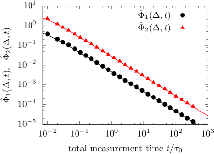
Figure 1: (color online) Correlation functions $\hat{\Phi}_{i}(t)\,(i=1,2)$ of the TMSD tensor calculated from trajectory data $\bm{R}_{G}(t)$ of the Rouse model (circles and triangles). The COM trajectories $\bm{R}_{G}(t)$ are generated through numerical simulations of the Rouse model. Time is measured in units of $\tau_{0}:=b^{2}/D$, where $b$ is the bond length, and $D$ is the diffusion constant of the beads. The number $N$ of beads and the lag time $\Delta$ are set as $N=50$ and $\Delta=0.01\tau_{0}$. The solid lines are the theoretical predictions given by Eqs. (45) and (46). There are no fitting parameters (the same is true of Figs. 2–4).

In Fig. 1, these formulas [Eqs. (45) and (46)] are displayed by the solid lines, and results of the numerical simulations by the circles and the triangles; the theoretical curves are in excellent agreement with the simulation results. These numerical results were obtained from trajectory data $\bm{R}_{G}(t)$ that were generated through Brownian dynamics simulations of the Rouse model [Eq. (43)].

V Zimm model

In this section, we study the Zimm model without the excluded volume interaction (i.e., the Zimm model in the $\Theta$ condition). Some scaling properties of the Rouse model are known to be inconsistent with experiments Doi and Edwards (1986), which is because the hydrodynamic interaction is disregarded entirely in the Rouse model. In contrast, the hydrodynamic interaction is taken into account in the Zimm model, which is another model of a flexible polymer chain in dilute solutions.

V.1 Model definition

As in the case of the Rouse model, the Zimm model consists of $N$ equivalent beads, and the equation of motion for bead $n$ is given by Zimm (1956); Doi and Edwards (1986); Ermak and McCammon (1978)

$$\frac{\partial\bm{R}_{n}(t)}{\partial t}=k\sum_{m}\bm{H}_{nm}\cdot\frac{\partial^{2}\bm{R}_{m}(t)}{\partial m^{2}}+\bm{f}_{n}(t),$$ (47)

where the hydrodynamic interaction is represented in terms of the mobility matrix $\bm{H}_{nm}$ defined by

$$\bm{H}_{nn} :=\frac{\bm{I}}{6\pi\eta a},$$ (48)

$$\bm{H}_{nm} :=\frac{1}{8\pi\eta r_{nm}}\left(\bm{I}+\frac{\bm{r}_{nm}{\bm{r}}_{nm}}{r_{nm}^{2}}\right)\quad(n\neq m).$$ (49)

Here, $\eta$ is the viscosity of the solvent and $a$ is the radius of each bead. Moreover, $\bm{r}_{nm}(t)$ and $r_{nm}(t)$ are defined as $\bm{r}_{nm}(t):=\bm{R}_{n}(t)-\bm{R}_{m}(t)$ and $r_{nm}(t):=|\bm{r}_{nm}(t)|$, respectively. The thermal noise $\bm{f}_{m}(t)$ satisfies the fluctuation-dissipation relation

$$\left\langle\bm{f}_{n}(t)\bm{f}_{m}(t^{\prime})\right\rangle=2k_{B}T\bm{H}_{nm}\delta(t-t^{\prime}).$$ (50)

The non-diagonal elements $\bm{H}_{nm}$ [Eq. (49)] are known collectively as the Oseen tensor, the nonlinearity of which makes theoretical analysis of the Zimm model considerably difficult.

A simple approximation that is commonly adopted is a pre-averaging approximation Doi and Edwards (1986) in which $\bm{H}_{nm}$ is replaced with its equilibrium average $\left\langle\bm{H}_{nm}\right\rangle=:h(n-m)\bm{I}$. In this approximation, the equation of motion for bead $n$ is expressed as

$$\frac{\partial\bm{R}_{n}(t)}{\partial t}\approx k\sum_{m}h(n-m)\frac{\partial^{2}\bm{R}_{m}}{\partial m^{2}}+\tilde{\bm{f}}_{m}(t),$$ (51)

$$\bigl{\langle}\tilde{\bm{f}}_{n}(t)\tilde{\bm{f}}_{m}(t^{\prime})\bigr{\rangle}=2k_{B}Th(n-m)\bm{I}\delta(t-t^{\prime}).$$ (52)

Although this approximation works well for predicting the MSD of the COM motion Rey et al. (1989), it is impossible to use it to elucidate the fluctuating diffusivity. This is because the fluctuating diffusivity is disregarded entirely when replacing $\bm{H}_{nm}(t)$ in Eq. (50) with $h(n-m)\bm{I}$ [see Eq. (52)].

V.2 Equation of COM motion

To elucidate the effect of the fluctuating diffusivity, the pre-averaging approximation is applied to the internal modes only, whereas the COM motion is treated without pre-averaging.

The normal mode $\bm{X}_{p}(t)$ ($p=0,1,\dots$) of $\bm{R}_{n}(t)$ is defined by Doi and Edwards (1986)

$$\bm{X}_{p}(t):= \frac{1}{N}\int_{0}^{N}dn\cos\left(\frac{p\pi n}{N}\right)\bm{R}_{n}(t),$$ (53)

$$\bm{R}_{n}(t)= \bm{X}_{0}(t)+2\sum_{p=1}^{\infty}\cos\left(\frac{p\pi n}{N}\right)\bm{X}_{p}(t).$$ (54)

Note here that $\bm{X}_{0}(t)$ is equivalent to the COM position: $\bm{X}_{0}(t)=\bm{R}_{G}(t)$. Under the pre-averaging approximation [Eqs. (51) and (52)], the equations of motion for the normal modes are given by

$$\frac{\partial\bm{X}_{0}(t)}{\partial t} =\frac{\partial\bm{R}_{G}(t)}{\partial t}=\hat{\bm{f}}_{0}(t),$$ (55)

$$\frac{\partial\bm{X}_{p}(t)}{\partial t} =-\frac{\bm{X}_{p}(t)}{\tau_{p}}+\hat{\bm{f}}_{p}(t)\quad(p=1,2,\dots),$$ (56)

where $\hat{\bm{f}}_{p}(t)$ are random forces defined by

$$\left\langle\hat{\bm{f}}_{p}(t)\hat{\bm{f}}_{q}(t^{\prime})\right\rangle=2k_{B}T\hat{h}_{pq}\delta(t-t^{\prime})\bm{I}\quad(p,q=0,1,\dots),$$ (57)

with

$$\hat{h}_{pq}:=\frac{1}{N^{2}}\int_{0}^{N}\!\!\!dn\int_{0}^{N}\!\!\!dm\cos\left(\frac{p\pi n}{N}\right)\cos\left(\frac{q\pi m}{N}\right)h(n-m).$$ (58)

For $p\neq 0$, $\hat{h}_{pq}$ can be approximated further as $\hat{h}_{pq}\approx{\delta_{pq}}/{\zeta_{p}}$, where $\zeta_{p}:=(12\pi^{3}pN)^{1/2}\eta b$ Doi and Edwards (1986). Consequently, the Langevin equations for the internal modes, Eq. (56), are mutually independent because

$$\left\langle\hat{\bm{f}}_{p}(t)\hat{\bm{f}}_{q}(t^{\prime})\right\rangle=\frac{2k_{B}T}{\zeta_{p}}\delta_{pq}\delta(t-t^{\prime})\bm{I}\quad(p=1,2,\dots).$$ (59)

Moreover, in Eq. (56), $\tau_{p}$ is the relaxation time of the $p$-th mode, and given by

$$\tau_{p}=\frac{\eta b^{3}}{k_{B}T}\sqrt{\frac{N^{3}}{3\pi p^{3}}}=\frac{\tau_{1}}{p^{3/2}}\quad(p=1,2,\dots),$$ (60)

where $\tau_{1}$ is the longest relaxation time.

Here, the COM equation of motion in Eq. (55) is rewritten as

$$\frac{\partial\bm{R}_{G}(t)}{\partial t}=\sqrt{2}\bm{B}(t)\cdot\bm{\xi}(t),$$ (61)

where $\bm{\xi}(t)$ is the white Gaussian noise given by Eq. (3). By comparing Eq. (61) with Eqs. (55), (57), and (58), $\bm{B}(t)$ is given by

$$\bm{D}(t)=\bm{B}(t)\cdot\bm{B}^{T}(t)=\frac{k_{B}T}{N^{2}}\int_{0}^{N}dn\int_{0}^{N}dm\bm{H}_{nm}(t),$$ (62)

where we restored the time dependence of the diffusivity by formally replacing $h(n-m)\bm{I}$ with $\bm{H}_{nm}(t)$. In the following analysis, Eqs. (56) and (59) are used for the internal modes, whereas Eqs. (61) and (62) are used for the COM motion. Thus, the diffusion coefficient of the Zimm model, in contrast to that of the Rouse model, depends on time $t$ and fluctuates because of the hydrodynamic interaction.

From Eqs. (49) and (62), we have the ensemble average of the diffusion coefficient tensor as

$$\left\langle\bm{D}\right\rangle= \frac{c\bm{I}}{3}\int_{0}^{N}dn\int_{0}^{N}dm\left\langle\frac{1}{r_{nm}}\right\rangle,$$ (63)

where $c:={k_{B}T}/(2\pi\eta N^{2})$ is a constant and we used the mutual independence of the magnitude $r_{nm}$ and direction $\bm{r}_{nm}/r_{nm}$ as follows Doi and Edwards (1986):

$$\left\langle\frac{1}{r_{nm}}\left(\bm{I}+\frac{\bm{r}_{nm}{\bm{r}}_{nm}}{r_{nm}^{2}}\right)\right\rangle =\frac{4}{3}\bm{I}\left\langle\frac{1}{r_{nm}}\right\rangle.$$ (64)

From Eq. (63), we have

$$\mathrm{tr}\left\langle\bm{D}\right\rangle =c\int_{0}^{N}dn\int_{0}^{N}dm\left\langle\frac{1}{r_{nm}}\right\rangle,$$ (65)

$$\mathrm{tr}\left(\left\langle\bm{D}\right\rangle\cdot\left\langle\bm{D}\right\rangle\right) =\frac{1}{3}\left(\mathrm{tr}\left\langle\bm{D}\right\rangle\right)^{2}.$$ (66)

The validity of Eq. (65) has been studied intensively Liu and Dünweg (2003), and it is shown that Eq. (65) is equivalent to the short-time diffusion coefficient of the COM and that it is also a good approximation to the long-time diffusion coefficient. In the next subsection, however, we have to study the second moment of the diffusion coefficient $\bm{D}(t)$.

Here, $\bm{r}_{nm}(t)$ follows three-dimensional Gaussian distribution with a covariant matrix $\bm{\Sigma}_{3}=\bm{I}|n-m|b^{2}/3$,

$$f_{3}(\bm{r})=\frac{1}{(2\pi|n-m|b^{2}/3)^{3/2}}\exp\left[-\frac{1}{2}\bm{r}\cdot\bm{\Sigma}_{3}^{-1}\cdot\bm{r}\right].$$ (67)

Thus, $\left\langle 1/r_{nm}(t)\right\rangle$ is obtained by integrating over $f_{3}(\bm{r})$ in spherical coordinates as Doi and Edwards (1986)

$$\left\langle\frac{1}{r_{nm}}\right\rangle=\left(\frac{6}{\pi b^{2}|n-m|}\right)^{1/2}.$$ (68)

From Eqs. (63) and (68), we have an explicit expression of the ensemble-averaged diffusivity,

$$\left\langle\bm{D}\right\rangle=\frac{8c}{3b}\left(\frac{2N^{3}}{3\pi}\right)^{1/2}\bm{I}.$$ (69)

It follows that

$$\mathrm{tr}\left\langle\bm{D}\right\rangle =\frac{8c}{b}\left(\frac{2N^{3}}{3\pi}\right)^{1/2},$$ (70)

$$\mathrm{tr}(\left\langle\bm{D}\right\rangle\cdot\left\langle\bm{D}\right\rangle) =\left(\frac{8c}{b}\right)^{2}\frac{2N^{3}}{9\pi}.$$ (71)

V.3 Correlation functions of diffusion coefficient

In this subsection, we calculate the magnitude and orientation correlation functions $\phi_{1}(t)$ and $\phi_{2}(t)$, respectively, of the diffusivity [Eqs. (27) and (28)]. In the following derivation, we use crude approximations such as a single-mode approximation and a perturbation expansion of the Gaussian distribution. Nevertheless, the final results exhibit relatively good agreement with those of numerical simulations.

V.3.1 Magnitude correlation function of diffusion coefficient

We begin by deriving the magnitude correlation function $\phi_{1}(t)$ of the diffusivity. From Eqs. (49) and (62), we have

$$\left\langle\mathrm{tr}\bm{D}(t)\mathrm{tr}\bm{D}(0)\right\rangle=$$

$$\hskip 8.5359ptc^{2}\int_{0}^{N}\!\!\!dn\!\int_{0}^{N}\!\!\!dm\!\int_{0}^{N}\!\!\!dn^{\prime}\!\int_{0}^{N}\!\!\!dm^{\prime}\!\left\langle\frac{1}{r_{nm}(t)r_{n^{\prime}m^{\prime}}(0)}\right\rangle.$$ (72)

To evaluate the ensemble average in the integrand, we define a six-dimensional vector $\bm{X}:=(x,x^{\prime},y,y^{\prime},z,z^{\prime})$, where $(x,y,z):=\bm{r}_{nm}(t)$ and $(x^{\prime},y^{\prime},z^{\prime}):=\bm{r}_{n^{\prime}m^{\prime}}(0)$. It can be shown that $\bm{X}$ follows six-dimensional Gaussian distribution (see Appendix B for a derivation), namely

$$f_{6}(\bm{X})=\frac{1}{(2\pi)^{3}\left|\bm{\Sigma}_{6}\right|^{1/2}}\exp\left[-\frac{1}{2}\bm{X}\cdot\bm{\Sigma}_{6}^{-1}\cdot\bm{X}\right].$$ (73)

Here, $\bm{\Sigma}_{6}$ is a $6\times 6$ covariant matrix defined by

$$\bm{\Sigma}_{6}:=\begin{pmatrix}\bm{A}&\bm{0}&\bm{0}\\[0.0pt] \bm{0}&\bm{A}&\bm{0}\\[0.0pt] \bm{0}&\bm{0}&\bm{A}\\[0.0pt] \end{pmatrix},\qquad\bm{A}:=\begin{pmatrix}\alpha&\beta\\ \beta&\alpha^{\prime}\end{pmatrix},$$ (74)

where $\bm{0}$ is the $2\times 2$ zero matrix; $\alpha,\alpha^{\prime}$ and $\beta$ are defined by (see Appendix B)

$$\alpha= \frac{b^{2}}{3}|n-m|,\qquad\alpha^{\prime}=\frac{b^{2}}{3}|n^{\prime}-m^{\prime}|,$$ (75)

$$\beta= \frac{8Nb^{2}}{3\pi^{2}}\sum_{p=1}^{\infty}\frac{e^{-t/\tau_{p}}}{p^{2}}\sin\frac{p\pi(n+m)}{2N}\sin\frac{p\pi(n-m)}{2N}$$

$$\hskip 48.36958pt\times\sin\frac{p\pi(n^{\prime}+m^{\prime})}{2N}\sin\frac{p\pi(n^{\prime}-m^{\prime})}{2N}.$$ (76)

Hereinafter, we take only the longest relaxation mode ($p=1$) into account and ignore all the other modes (i.e., a single-mode approximation):

$$\beta\approx\frac{8Nb^{2}}{3\pi^{2}}e^{-t/\tau_{1}} \sin\frac{\pi(n+m)}{2N}\sin\frac{\pi(n-m)}{2N}$$

$$\times \sin\frac{\pi(n^{\prime}+m^{\prime})}{2N}\sin\frac{\pi(n^{\prime}-m^{\prime})}{2N}.$$ (77)

Consequently, the determinant of the covariant matrix $\bm{\Sigma}_{6}$ is given by

$$\left|\bm{\Sigma}_{6}\right|=\left(\alpha\alpha^{\prime}-\beta^{2}\right)^{3}=\left(\alpha\alpha^{\prime}\right)^{3}\left(1-\epsilon\right)^{3}=\left(\tilde{\alpha}\alpha^{\prime}\right)^{3},$$ (78)

where $\epsilon:=\beta^{2}/(\alpha\alpha^{\prime})$ and $\tilde{\alpha}:=\alpha(1-\epsilon)$.

Using these quantities in Eq. (73), we have

$$\left\langle\frac{1}{r_{nm}(t)r_{n^{\prime}m^{\prime}}(0)}\right\rangle =$$

$$\frac{\tilde{\alpha}\tilde{\alpha}^{\prime}}{(2\pi)^{3}\left|\bm{\Sigma}_{6}\right|^{1/2}}\int d\bm{r}\int d\bm{r}^{\prime}\frac{1}{rr^{\prime}}e^{-\frac{r^{2}}{2}-\frac{r^{\prime 2}}{2}+\epsilon^{1/2}\bm{r}\cdot\bm{r}^{\prime}},$$ (79)

where $\bm{r}:=(x,y,z)$, and $\bm{r}^{\prime}:=(x^{\prime},y^{\prime},z^{\prime})$. For $t\gg\tau_{1}$, we have $\epsilon\ll 1$ and the above integrand can be approximated further as

$$e^{\epsilon^{1/2}\bm{r}\cdot\bm{r}^{\prime}}\simeq\quad 1+\epsilon^{1/2}\bm{r}\cdot\bm{r}^{\prime}+\frac{\epsilon}{2}(\bm{r}\cdot\bm{r}^{\prime})^{2}.$$ (80)

Integrating Eq. (79) in spherical coordinates, we have a perturbation expansion upto order $\epsilon^{1}$ as

$$\left\langle\frac{1}{r_{nm}(t)r_{n^{\prime}m^{\prime}}(0)}\right\rangle \simeq\frac{2}{\pi(\alpha\alpha^{\prime})^{1/2}}\left(1+\frac{\epsilon}{6}\right)$$

$$=\left\langle\frac{1}{r_{nm}}\right\rangle\left\langle\frac{1}{r_{n^{\prime}m^{\prime}}}\right\rangle+\frac{\epsilon}{3\pi(\alpha\alpha^{\prime})^{1/2}},$$ (81)

where we used Eqs. (68) and (75). Inserting this equation into Eq. (V.3.1) and taking Eq. (65) into account, we obtain

$$\left\langle\mathrm{tr}\bm{D}(t)\mathrm{tr}\bm{D}(0)\right\rangle -\left(\mathrm{tr}\left\langle\bm{D}\right\rangle\right)^{2}$$

$$= \frac{c^{2}}{3\pi}\int_{0}^{N}\!\!\!dn\!\int_{0}^{N}\!\!\!dm\!\int_{0}^{N}\!\!\!dn^{\prime}\!\int_{0}^{N}\!\!\!dm^{\prime}\frac{\epsilon}{(\alpha\alpha^{\prime})^{1/2}}$$

$$= \left(\frac{8c}{b}\right)^{2}\frac{N^{3}K^{2}}{\pi^{6}}e^{-2t/\tau_{1}},$$ (82)

where $K$ is a constant defined by

$$K:=\int_{0}^{\pi}d\xi\,\frac{\sin^{2}\frac{\xi}{2}}{\xi^{3/2}}\left(\pi-\xi+\sin\xi\right)\approx 1.428226.$$ (83)

Finally, from Eqs. (70) and (V.3.1), we have the magnitude correlation function $\phi_{1}(t)$ of the diffusivity [Eq. (27)] as

$$\phi_{1}(t)=\frac{3K^{2}}{2\pi^{5}}e^{-2t/\tau_{1}}.$$ (84)

V.3.2 Orientation correlation function of diffusion coefficient

We move on to a derivation of the orientation correlation function $\phi_{2}(t)$ of the diffusivity [Eq. (28)]. From Eqs. (49) and (62), we have

$$\mathrm{tr}\left\langle\bm{D}(t)\cdot\bm{D}(0)\right\rangle= \frac{c^{2}}{16}\int_{0}^{N}\!\!\!dn\!\int_{0}^{N}\!\!\!dm\!\int_{0}^{N}\!\!\!dn^{\prime}\!\int_{0}^{N}\!\!\!dm^{\prime}$$

$$\times\left\langle\frac{\left[\hat{\bm{r}}_{nm}(t)\cdot\hat{\bm{r}}_{n^{\prime}m^{\prime}}(0)\right]^{2}+5}{r_{nm}(t)r_{n^{\prime}m^{\prime}}(0)}\right\rangle,$$ (85)

where $\hat{\bm{r}}$ is the unit vector in the direction of $\bm{r}$. The ensemble average in Eq. (85) can be carried out in a way similar to the calculation of Eq. (79). In fact, under the approximation in Eq. (80), we obtain

$$\left\langle\frac{\left[\hat{\bm{r}}_{nm}(t)\cdot\hat{\bm{r}}_{n^{\prime}m^{\prime}}(0)\right]^{2}+5}{r_{nm}(t)r_{n^{\prime}m^{\prime}}(0)}\right\rangle =\frac{16}{3}\frac{2}{\pi(\alpha\alpha^{\prime})^{1/2}}\left(1+\frac{1}{5}\epsilon\right)$$

$$=\frac{16}{3}\left\langle\frac{1}{r_{nm}}\right\rangle\left\langle\frac{1}{r_{n^{\prime}m^{\prime}}}\right\rangle+\frac{32}{15}\frac{\epsilon}{\pi(\alpha\alpha^{\prime})^{1/2}}.$$ (86)

Inserting Eq. (86) into Eq. (85) and taking Eqs. (65) and (66) into account, we have

$$\mathrm{tr}\left\langle\bm{D}(t)\cdot\bm{D}(0)\right\rangle -\mathrm{tr}\left(\left\langle\bm{D}\right\rangle\cdot\left\langle\bm{D}\right\rangle\right)$$

$$= \frac{2c^{2}}{15\pi}\int_{0}^{N}\!\!\!dn\!\int_{0}^{N}\!\!\!dm\!\int_{0}^{N}\!\!\!dn^{\prime}\!\int_{0}^{N}\!\!\!dm^{\prime}\frac{\epsilon}{(\alpha\alpha^{\prime})^{1/2}}$$

$$= \frac{2}{5}\left(\frac{8c}{b}\right)^{2}\frac{N^{3}K^{2}}{\pi^{6}}e^{-2t/\tau_{1}},$$ (87)

Finally, from Eqs. (71) and (87), we have the orientation correlation function $\phi_{2}(t)$ of the diffusivity [Eq. (28)] as

$$\phi_{2}(t) =\frac{9K^{2}}{5\pi^{5}}e^{-2t/\tau_{1}}.$$ (88)

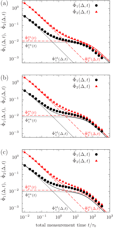
Figure 2: (color online) Correlation functions $\hat{\Phi}_{i}(t)\,(i=1,2)$ of the TMSD tensor calculated from trajectory data $\bm{R}_{G}(t)$ of the Zimm model (circles and triangles). The COM trajectories $\bm{R}_{G}(t)$ are generated through numerical simulations of the Zimm model (see Appendix C). Distance is measured in units of the bond length $b$ and time in units of $\tau_{0}:=b^{2}/D$, where $D$ is the diffusion coefficient of each bead. Results for three different values of the bead radius $a$ are presented: (a) $a=0.1b$, (b) $a=0.15b$ and (c) $a=0.2b$. The number $N$ of beads and the lag time $\Delta$ are set as $N=50$ and $\Delta=0.01\tau_{0}$. The longest relaxation time $\tau_{1}$ is estimated from Eq. (60) as (a) $\tau_{1}=61.0\tau_{0}$, (b) $\tau_{1}=40.7\tau_{0}$, and (c) $\tau_{1}=30.5\tau_{0}$. The dotted lines are the theoretical predictions for $\hat{\Phi}_{1}^{\mathrm{id}}(\Delta,t)$ and $\hat{\Phi}_{1}^{\mathrm{ex}}(t)$ given by Eqs. (89) and (90). The dashed lines are the theoretical predictions for $\hat{\Phi}_{2}^{\mathrm{id}}(\Delta,t)$ and $\hat{\Phi}_{2}^{\mathrm{ex}}(t)$ given by Eqs. (91) and (92). The solid lines are the sums $\hat{\Phi}_{i}(\Delta,t)\,\,(i=1,2)$ of the ideal and excess parts [Eqs. (24) and (34)].

V.4 Correlation functions of TMSD tensor

Here, we derive the correlation functions $\hat{\Phi}_{1}(\Delta,t)$ and $\hat{\Phi}_{2}(\Delta,t)$ of the TMSD tensor. From Eqs. (25), (26), (84), and (88), we have

$$\hat{\Phi}_{1}^{\mathrm{id}}(\Delta,t) =\frac{\Delta}{9t}\left(4-\frac{\Delta}{t}\right)\left(1+\frac{9K^{2}}{5\pi^{5}}\right),$$ (89)

$$\hat{\Phi}_{1}^{\mathrm{ex}}(\Delta,t) =\frac{3K^{2}\tau_{1}^{2}}{4\pi^{5}t^{2}}\left[\frac{2t}{\tau_{1}}+e^{-2t/\tau_{1}}-1\right],$$ (90)

where we used $C=1$ because the system is statistically isotropic. Similarly, from Eqs. (35), (36), (84), and (88), we obtain

$$\hat{\Phi}_{2}^{\mathrm{id}}(\Delta,t) =\frac{\Delta}{6t}\left(4-\frac{\Delta}{t}\right)\left(4+\frac{63K^{2}}{10\pi^{5}}\right),$$ (91)

$$\hat{\Phi}_{2}^{\mathrm{ex}}(\Delta,t) =\frac{6}{5}\hat{\Phi}_{1}^{\mathrm{ex}}(\Delta,t).$$ (92)

In contrast to the Rouse model, these correlation functions $\hat{\Phi}_{i}^{\mathrm{ex}}(t)$ $(i=1,2)$ for the Zimm model show crossovers. For example, from Eq. (42), $\hat{\Phi}_{1}^{\mathrm{ex}}(t)$ behaves as

$$\hat{\Phi}_{1}^{\mathrm{ex}}(t)\simeq\begin{cases}\frac{3K^{2}}{2\pi^{5}}&(t\ll\tau_{1}),\\[2.84544pt] \frac{3K^{2}\tau_{1}}{2\pi^{5}t}&(t\gg\tau_{1}).\end{cases}$$ (93)

From Eq. (93), the crossover time $\tau_{c}$ can be estimated as $\tau_{c}=\tau_{1}$, i.e., the crossover time is equivalent to the longest relaxation time $\tau_{1}$. Also, $\hat{\Phi}_{2}^{\mathrm{ex}}(t)$ shows a crossover at $t=\tau_{1}$, because of Eq. (92).

As can be seen in Fig. 2, the theoretical predictions (the solid lines) [Eqs. (89)–(92)] are in good agreement with the results of the numerical simulations (the symbols). The slight deviations are due to the approximations used in the theoretical analysis. For example, in the simulations, the Rotne-Prager-Yamakawa tensor [Eq. (132)] was utilized as the mobility matrix instead of the Oseen tensor [Eq. (49)] to regularize the singularity in the Oseen tensor at $r_{nm}=0$. Moreover, we also applied the pre-averaging approximation to the inner degrees of freedom, and used the perturbation expansion in Eq. (80). However, incorporating a higher order term ($\epsilon^{2}$) in Eq. (80) improves the theoretical predictions only slightly (its contribution is less than 15 % of the leading term; data not shown).

VI Discrete reptation model

In this section, the focus is on the discrete reptation model, which describes tagged polymer motion in entangled polymer solutions Doi and Edwards (1978, 1986). Because of the entanglement, the tagged polymer chain of the reptation model is temporarily trapped in a virtual tube comprised of surrounding chains, and moves only in the longitudinal direction of the tube. Such reptation dynamics are an essential ingredient in modeling DNA molecules at high concentration Gong and van der Maarel (2014).

In the reptation model, the centerline of the tube, which is called a primitive chain, is considered instead of the real chain of the tagged polymer. The primitive chain is assumed to consist of $N$ tube segments $\bm{R}_{1}(t),\dots,\bm{R}_{N}(t)$ connected by bonds of constant length $b$. The primitive chain is allowed to move only in the longitudinal direction of the tube as a result of the entanglement. A single step of the primitive-chain dynamics is given as follows; one of the two end segments, $\bm{R}_{1}(t)$ or $\bm{R}_{N}(t)$, is chosen with equal probability; the chosen end segment hops with step length $b$ in a random direction; and each of the other segments slides to one of the positions of its neighboring segments [i.e., if $\bm{R}_{1}(t)$ is chosen, $\bm{R}_{n}(t)$ slides to $\bm{R}_{n-1}(t)$ ($n=2,\dots,N$); if $\bm{R}_{N}(t)$ is chosen, $\bm{R}_{n}(t)$ slides to $\bm{R}_{n+1}(t)$ ($n=1,\dots,N-1$)].

The COM $\bm{R}_{G}(t)$ of this primitive chain follows the LEFD [Eq. (2)] with $\bm{B}(t)$ given by Doi and Edwards (1978); Uneyama et al. (2015)

$$\bm{B}(t)\approx\sqrt{\frac{3D_{G}}{\left\langle\bm{p}^{2}\right\rangle}}\frac{\bm{p}(t)\bm{p}(t)}{|\bm{p}(t)|},$$ (94)

where $D_{G}$ is the ensemble-averaged diffusion coefficient of the COM, and $\bm{p}(t)$ is the end-to-end vector of the primitive chain. It follows that the diffusion coefficient is obtained from Eq. (4) as

$$\bm{D}(t)=3D_{G}\frac{\bm{p}(t)\bm{p}(t)}{\left\langle\bm{p}^{2}\right\rangle}.$$ (95)

Because the system is statistically isotropic, $\left\langle\bm{p}\bm{p}\right\rangle=A\bm{I}$ with a constant $A$. Taking the trace, we have $A=\left\langle\bm{p}^{2}\right\rangle/3$. It follows that $\left\langle\bm{D}\right\rangle=D_{G}\bm{I}$.

By using Eqs. (27), (28) and (95), the magnitude and the orientation correlation functions $\phi_{1}(\tau)$ and $\phi_{2}(\tau)$ of the diffusivity can be expressed as

$$\phi_{1}(\tau) =\frac{\left\langle\bm{p}^{2}(\tau)\bm{p}^{2}(0)\right\rangle}{\left\langle\bm{p}^{2}\right\rangle^{2}}-1,$$ (96)

$$\phi_{2}(\tau) =3\frac{\langle\left[\bm{p}(\tau)\cdot\bm{p}(0)\right]^{2}\rangle}{\left\langle\bm{p}^{2}\right\rangle^{2}}-1.$$ (97)

In Ref. Uneyama et al. (2015), $\phi_{1}(\tau)$ was obtained explicitly as

$$\phi_{1}(\tau)=\frac{16}{3\pi^{2}}\sum_{k:\mathrm{odd}}\frac{1}{k^{2}}E_{2}\left(\frac{k^{2}\tau}{\tau_{d}}\right),$$ (98)

where $\tau_{d}$ is the longest relaxation time of the reptation model, and $E_{m}(x)$ is the generalized exponential integral of order $m$ Olver et al. (2010). Furthermore, it is shown in Appendix D that

$$\phi_{2}(\tau)=6\phi_{1}(\tau).$$ (99)

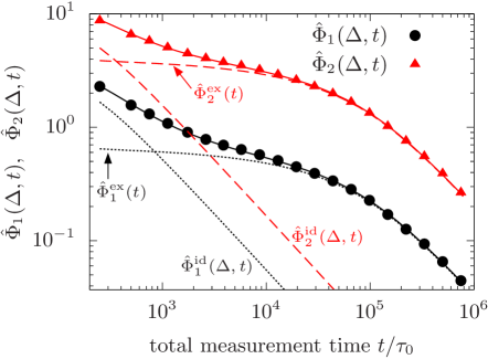
Figure 3: (color online) Correlation functions $\hat{\Phi}_{i}(t)\,(i=1,2)$ of the TMSD tensor calculated from trajectory data $\bm{R}_{G}(t)$ of the reptation model (circles and triangles). The COM trajectories $\bm{R}_{G}(t)$ are generated through numerical simulations of the reptation model. Distance is measured in units of the bond length $b$ between the tube segments, and time in units of $\tau_{0}:=b^{2}\zeta/k_{B}T$, where $\zeta$ is a friction coefficient of the tube segment. The number $N$ of tube segments and the lag time $\Delta$ are set as $N=85$ and $\Delta=250\tau_{0}$. For details of the simulation setup, see Ref. Uneyama et al. (2012). The longest relaxation time (a disengagement time) $\tau_{d}=N^{3}\tau_{0}/\pi^{2}$ is estimated as $\tau_{d}\approx 6.2\times 10^{4}\tau_{0}$. The dotted lines are the theoretical predictions for $\hat{\Phi}_{1}^{\mathrm{id}}(\Delta,t)$ and $\hat{\Phi}_{1}^{\mathrm{ex}}(t)$ given by Eqs. (100) and (101). The dashed lines are the theoretical predictions for $\hat{\Phi}_{2}^{\mathrm{id}}(\Delta,t)$ and $\hat{\Phi}_{2}^{\mathrm{ex}}(t)$ given by Eqs. (102) and (103). The solid lines are the sums $\hat{\Phi}_{i}(\Delta,t)\,\,(i=1,2)$ of the ideal and excess parts [Eqs. (24) and (34)].

From Eqs. (25) and (26), we have the correlation functions of the TMSD tensor as

$$\hat{\Phi}_{1}^{\mathrm{id}}(\Delta,t) =\frac{5\Delta}{9t}\left(4-\frac{\Delta}{t}\right),$$ (100)

$$\hat{\Phi}_{1}^{\mathrm{ex}}(\Delta,t) =\frac{\pi^{2}\tau_{d}}{18t}-\frac{\pi^{4}\tau_{d}^{2}}{270t^{2}}+\frac{32\tau_{d}^{2}}{3\pi^{2}t^{2}}\sum_{k:\mathrm{odd}}\frac{E_{4}\left(\frac{k^{2}t}{\tau_{d}}\right)}{k^{6}},$$ (101)

where we used $\phi_{2}(0)=6\phi_{1}(0)=4$. Similarly, from Eqs. (35), (36) and (99), we have

$$\hat{\Phi}_{2}^{\mathrm{id}}(\Delta,t) =\frac{5\Delta}{3t}\left(4-\frac{\Delta}{t}\right)=3\hat{\Phi}_{1}^{\mathrm{id}}(\Delta,t),$$ (102)

$$\hat{\Phi}_{2}^{\mathrm{ex}}(\Delta,t) =6\hat{\Phi}_{1}^{\mathrm{ex}}(\Delta,t).$$ (103)

As in the case of the Zimm model, both functions $\hat{\Phi}_{i}^{\mathrm{ex}}(t)$ $(i=1,2)$ show crossovers. For example, $\hat{\Phi}_{1}^{\mathrm{ex}}(t)$ behaves as Uneyama et al. (2015)

$$\hat{\Phi}_{1}^{\mathrm{ex}}(t)\simeq\begin{cases}\frac{2}{3}&(t\ll\tau_{d}),\\[2.84544pt] \frac{\pi^{2}\tau_{d}}{18t}&(t\gg\tau_{d}).\end{cases}$$ (104)

Also, $\hat{\Phi}_{2}^{\mathrm{ex}}(t)$ shows a crossover at $t=\tau_{d}$, because of Eq. (103). From Eq. (104), this crossover time can be estimated as

$$\tau_{c}=\frac{\pi^{2}}{12}\tau_{d},$$ (105)

which is close to the longest relaxation time $\tau_{d}$.

In Fig. 3, results of the numerical simulations for the discrete reptation model are displayed; they exhibit remarkable agreement with the theoretical predictions [Eqs. (100)–(103)]. Moreover, $\hat{\Phi}_{2}^{\mathrm{ex}}(\Delta,t)$ far exceeds $\hat{\Phi}_{1}^{\mathrm{ex}}(\Delta,t)$ in the reptation model, in contrast to the Zimm model for which the two functions are comparable. This means that the orientation fluctuation of the diffusivity is more prominent in the reptation model than in the Zimm model.

VII Rigid rod-like polymer

Finally, the rigid rod-like polymer in a dilute condition is investigated as an extreme example of non-flexible polymers Burgers (1995); Doi and Edwards (1986); Dhont (1996); Berne and Pecora (2000). In general, it is more difficult to observe rotational diffusion of an anisotropic particle than it is to observe its translational diffusion Han et al. (2006). With the TMSD tensor analysis, however, the rotational diffusion coefficient can be estimated by measuring translational motion of the COM.

Let us denote the COM of the rod as $\bm{R}_{G}(t)$, and assume that the rod is cylindrically symmetric along the long axis. Consequently, the COM position $\bm{R}_{G}(t)$ follows the LEFD [Eq. (2)] with $\bm{B}(t)$ given (see Appendix E) by

$$\bm{B}(t)=\sqrt{D_{\parallel}}\hat{\bm{u}}(t)\hat{\bm{u}}(t)+\sqrt{D_{\perp}}\left[\bm{I}-\hat{\bm{u}}(t)\hat{\bm{u}}(t)\right],$$ (106)

where $\hat{\bm{u}}(t)$ is a unit vector in the direction of the rod’s long axis, and $D_{\parallel}$ and $D_{\perp}$ are the diffusion coefficients along and perpendicular to the long axis, respectively. Moreover, it is assumed that the rod is long and thin so that rotational motion around the long axis is disregarded. The time evolution of the rod’s direction $\hat{\bm{u}}(t)$ is given by Dhont (1996)

$$\frac{d\hat{\bm{u}}(t)}{dt} =\sqrt{2D_{r}}\bm{\eta}(t)\times\hat{\bm{u}}(t),$$ (107)

$$\left\langle\bm{\eta}(t)\right\rangle=0, \quad\left\langle\bm{\eta}(t)\bm{\eta}(t^{\prime})\right\rangle=\bm{I}\delta(t-t^{\prime}),$$ (108)

where $\bm{\eta}(t)$ is white Gaussian noise, and $D_{r}$ is the rotational diffusion coefficient. The three diffusion coefficients $D_{\parallel}$, $D_{\perp}$ and $D_{r}$ can be expressed in terms of the length $L$ and diameter $b$ of the rod as Doi and Edwards (1986); Dhont (1996)

$$D_{\parallel}=2D_{\perp} =\frac{k_{B}T\ln(L/b)}{2\pi\eta L},$$ (109)

$$D_{r} =\frac{3k_{B}T\ln(L/b)}{\pi\eta L^{3}}.$$ (110)

These formulas are obtained through hydrodynamic calculations for a long thin rod, i.e., $L/b\gg 1$.

Firstly, we consider the magnitude correlation function $\hat{\Phi}_{1}(t)$. From Eqs. (4) and (106), we have the fluctuating diffusivity as

$$\bm{D}(t)=D_{\parallel}\hat{\bm{u}}(t)\hat{\bm{u}}(t)+D_{\perp}\left[\bm{I}-\hat{\bm{u}}(t)\hat{\bm{u}}(t)\right].$$ (111)

Taking the trace, we obtain $\mathrm{tr}\bm{D}(t)=D_{\parallel}+2D_{\perp}$, i.e., the magnitude of the diffusivity is constant in time. It follows that the magnitude correlation of the diffusivity vanishes, i.e., $\phi_{1}(\tau)\equiv 0$; hence we have from Eq. (26) that

$$\hat{\Phi}_{1}^{\mathrm{ex}}(t)\equiv 0.$$ (112)

Thus, for the rigid rod-like polymer, in contrast to the Zimm and reptation models, it is impossible to extract information about the fluctuating diffusivity by using $\hat{\Phi}_{1}(t)$ .

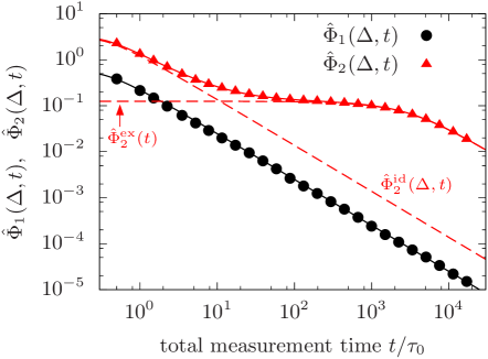
Figure 4: (color online) Correlation functions $\hat{\Phi}_{i}(t)\,(i=1,2)$ of the TMSD tensor calculated from trajectory data $\bm{R}_{G}(t)$ of the rigid rod-like polymer (circles and triangles). The COM trajectories $\bm{R}_{G}(t)$ are generated through numerical simulations of the rigid rod-like polymer [Eqs. (2), (106), and (107)]. Distance is measured in units of the rod’s diameter $b$ and time in units of $\tau_{0}:=b^{3}\eta/k_{B}T$. The length $L$ of the rod is set as $L=30b$, and $\Delta$ is $0.5\tau_{0}$. The values of the three diffusion coefficients ($D_{\perp},D_{\parallel},D_{r}$) are given by Eqs. (109) and (110). In particular, the rotational relaxation time $1/D_{r}$ is estimated from Eq. (110) as $1/D_{r}\approx 8.3\times 10^{3}\tau_{0}$. The dashed lines are the theoretical predictions for $\hat{\Phi}_{2}^{\mathrm{id}}(\Delta,t)$ and $\hat{\Phi}_{2}^{\mathrm{ex}}(t)$ given by Eqs. (118) and (116). The solid lines are the sums $\hat{\Phi}_{i}(\Delta,t)\,\,(i=1,2)$ of the ideal and excess parts [Eqs. (24) and (34)].

Therefore, to elucidate the fluctuating diffusivity of the rod, it is necessary to study $\hat{\Phi}_{2}(t)$. From Eqs. (28) and (111), we obtain the orientation correlation function as

$$\phi_{2}(\tau)=\left(\frac{D_{\parallel}-D_{\perp}}{D_{\parallel}+2D_{\perp}}\right)^{2}\left\{3\left\langle\bigl{[}\hat{\bm{u}}(\tau)\cdot\hat{\bm{u}}(0)\bigr{]}^{2}\right\rangle-1\right\},$$ (113)

where we used $\left\langle\bm{D}\right\rangle=(D_{\parallel}+2D_{\perp})\bm{I}/3$. Because the rotational motion given by Eq. (107) is independent of the translational motion $\bm{R}_{G}(t)$, the correlation function $\langle[\hat{\bm{u}}(\tau)\cdot\hat{\bm{u}}(0)]^{2}\rangle$ can be calculated by employing the Smoluchowsky equation for the rotational motion as Doi and Edwards (1986); Berne and Pecora (2000)

$$\left\langle\bigl{[}\hat{\bm{u}}(\tau)\cdot\hat{\bm{u}}(0)\bigr{]}^{2}\right\rangle=\frac{1}{3}\left(1+2e^{-6D_{r}t}\right),$$ (114)

and hence we have

$$\phi_{2}(\tau)=2\left(\frac{D_{\parallel}-D_{\perp}}{D_{\parallel}+2D_{\perp}}\right)^{2}e^{-6D_{r}\tau}.$$ (115)

From Eq. (36), the excess part $\hat{\Phi}_{2}^{\mathrm{ex}}(t)$ of the orientation correlation function is obtained as

$$\hat{\Phi}_{2}^{\mathrm{ex}}(t)=\frac{1}{9D_{r}^{2}t^{2}}\left(\frac{D_{\parallel}-D_{\perp}}{D_{\parallel}+2D_{\perp}}\right)^{2}\left(6D_{r}t+e^{-6D_{r}t}-1\right).$$ (116)

Moreover, by using Eqs. (25) and (35), the ideal parts are given by

$$\hat{\Phi}_{1}^{\mathrm{id}}(t) =\frac{\Delta}{9t}\left(4-\frac{\Delta}{t}\right)\left[1+2\left(\frac{D_{\parallel}-D_{\perp}}{D_{\parallel}+2D_{\perp}}\right)^{2}\right],$$ (117)

$$\hat{\Phi}_{2}^{\mathrm{id}}(t) =\frac{\Delta}{3t}\left(4-\frac{\Delta}{t}\right)\left[2+\left(\frac{D_{\parallel}-D_{\perp}}{D_{\parallel}+2D_{\perp}}\right)^{2}\right],$$ (118)

where $C=1$ is used because the system is statistically isotropic. In particular, from Eq (42), we have the following crossover:

$$\hat{\Phi}_{2}^{\mathrm{ex}}(t)\approx\begin{cases}2\left(\frac{D_{\parallel}-D_{\perp}}{D_{\parallel}+2D_{\perp}}\right)^{2}&(t\ll 1/D_{r}),\\[2.84544pt] \frac{2}{3D_{r}t}\left(\frac{D_{\parallel}-D_{\perp}}{D_{\parallel}+2D_{\perp}}\right)^{2}&(t\gg 1/D_{r}).\end{cases}$$ (119)

An estimate for the rotational relaxation time $1/D_{r}$ can be obtained from this crossover time, despite the fact that we observe only the translational motion of the rod. In fact, we have the crossover time $\tau_{c}$ from Eq. (119) as

$$\tau_{c}=\frac{1}{3D_{r}}.$$ (120)

Thus, the crossover time $\tau_{c}$ gives an estimate of the rotational relaxation time $1/D_{r}$.

Results of the numerical simulations for $\hat{\Phi}_{1}(t)$ and $\hat{\Phi}_{2}(t)$ are presented in Fig. 4 (the circles and triangles). As predicted, $\hat{\Phi}_{1}(t)$ shows no crossover because the excess part is absent, whereas $\hat{\Phi}_{2}(t)$ exhibits a clear crossover. The numerical results are consistent with the theoretical predictions (the solid lines).

VIII Discussion

The sample-to-sample fluctuation of the diffusivity observed both in SPT experiments and theoretical models has been studied intensively for a decade. In such studies, the sample-to-sample fluctuation is usually characterized by the EB parameter He et al. (2008); Deng and Barkai (2009); Jeon et al. (2011); Tabei et al. (2013); Metzler et al. (2014); Miyaguchi and Akimoto (2011, 2013); Thiel and Sokolov (2014a, b); Uneyama et al. (2012, 2015); Miyaguchi and Akimoto (2015); Miyaguchi et al. (2016). However, when calculating the EB parameter from trajectory data $\bm{r}(t)$, much of the information originally contained in the data is lost. In this study, to obtain more information from the trajectory data, the EB parameter is generalized into the fourth-order tensor $\bm{\Phi}(\Delta,t)$, which is a correlation function of the TMSD tensor. Moreover, the two scalar functions $\hat{\Phi}_{1}(\Delta,t)$ and $\hat{\Phi}_{2}(\Delta,t)$ are derived from $\bm{\Phi}(\Delta,t)$; these functions are closely related to the magnitude and orientation correlation functions of the diffusivity, and in particular $\hat{\Phi}_{1}(\Delta,t)$ is equivalent to the EB parameter. It is also worth noting that a linear combination of the excess parts $\hat{\Phi}_{1}^{\mathrm{ex}}(\Delta,t)$ and $\hat{\Phi}_{2}^{\mathrm{ex}}(\Delta,t)$ gives the non-Gaussian parameter $A(t)$ [Eq. (38)]. In other words, the non-Gaussianity can be decomposed into two parts: one originating from the magnitude fluctuation of the diffusivity, and the other from the orientation fluctuation.

Furthermore, by using the TMSD tensor analysis, it is shown that the four polymer models exhibit distinctly different types of fluctuating diffusivity in terms of the correlation functions $\hat{\Phi}_{1}^{\mathrm{ex}}(\Delta,t)$ and $\hat{\Phi}_{2}^{\mathrm{ex}}(\Delta,t)$. For example, $\hat{\Phi}_{1}^{\mathrm{ex}}(\Delta,t)\approx\hat{\Phi}_{2}^{\mathrm{ex}}(\Delta,t)$ in the Zimm model, $\hat{\Phi}_{1}^{\mathrm{ex}}(\Delta,t)<\hat{\Phi}_{2}^{\mathrm{ex}}(\Delta,t)$ in the reptation model, and $\hat{\Phi}_{1}^{\mathrm{ex}}(\Delta,t)\ll\hat{\Phi}_{2}^{\mathrm{ex}}(\Delta,t)$ in the rigid rod-like polymer. This is in contrast to the non-Gaussian parameter $A(t)$, whose behavior is qualitatively similar for these three models; hence the polymer models are barely distinguishable with $A(t)$.

From these results, it seems that the fluctuating diffusivity might be ubiquitous in polymer motions from dilute to concentrated solutions and from flexible to non-flexible polymers. This is because the Zimm and the reptation models are flexible polymer models in dilute and concentrated solutions, respectively; in contrast, the rigid rod-like polymer is an extreme case of non-flexible polymers; each of these three models exhibits fluctuating diffusivity.

Moreover, the rotational relaxation time $\tau_{r}=1/D_{r}$ of the rigid rod can be obtained from the crossover time of $\hat{\Phi}_{2}^{\mathrm{ex}}(t)$ [Eq. (119)]. As a more direct approach, $\tau_{r}=1/D_{r}$ of an anisotropic particle was obtained in Ref. Han et al. (2006) by measuring the particle’s direction. Also, with the results of Refs. Brenner (1963); Cichocki et al. (2012), $\tau_{r}$ of the rigid rod can be estimated from the ensemble-averaged MSD of a reference point on the rod other than its COM. For both methods, however, it is necessary to measure at least one reference point other than the COM. In contrast, with the method proposed here, $\tau_{r}$ can be estimated by measuring only the translational motion of the COM.

Of course, the same information of $\hat{\Phi}_{1}^{\mathrm{ex}}(t)$ and $\hat{\Phi}_{2}^{\mathrm{ex}}(t)$ would be obtained from the ensemble-averaged quantities. In fact, the functions $\hat{\Phi}_{1}^{\mathrm{ex}}(t)$ and $\hat{\Phi}_{2}^{\mathrm{ex}}(t)$ are related to the non-Gaussian parameter $A(t)$ [Eq. (38)], which is defied by a fourth moment. Thus, essentially the same information as $\hat{\Phi}_{1}^{\mathrm{ex}}(t)$ and $\hat{\Phi}_{2}^{\mathrm{ex}}(t)$ might well be obtained from the translational correlation tensor of fourth order, which might be analyzed by the traditional approach with the Smoluchowski equation Rallison (1978); Cichocki et al. (2012, 2015). However, It should be noted that to calculate fourth moments such as $A(t)$ accurately, a large number of trajectories are necessary in general. In contrast, the present method, in which the time and ensemble averages are combined, works for a relatively small number of trajectories (typically, from tens to hundreds of trajectories), and therefore it would be useful in single-particle-tracking experiments, in which much effort is required to obtain a large number of trajectories.

Although the TMSD tensor analysis for the polymer models is based on the fact that the COM of these models can be described in terms of the LEFD [Eq. (2)], there are many phenomena that cannot be described with the LEFD. For example, the motion of a single bead in the Zimm and reptation models does not follow the LEFD because the bead shows anomalous subdiffusion, whereas the LEFD exhibits only normal diffusion as shown in Eq. (7). A candidate for describing such complex dynamics might be a generalized Langevin equation or fractional Brownian motion with fluctuating diffusivity, but the physical validity of such models should be clarified in future work.

Moreover, only two scalar functions, namely $\hat{\Phi}_{1}(\Delta,t)$ and $\hat{\Phi}_{2}(\Delta,t)$, were used here to analyze the isotropic polymer models. However, there must still be useful information in the fourth-order tensor $\bm{\Phi}(\Delta,t)$ for the case of anisotropic systems (see Sec. III.5). Future work should therefore include a full characterization of this tensor $\bm{\Phi}(\Delta,t)$.

Appendix A Decomposition of fourth-order tensor $\bm{\Phi}(\Delta,t)$ into ideal and excess parts

In this appendix, the expression for $\bm{\Psi}^{1}(\Delta,t)$ given in Eq. (III.2) is derived. First, using Eqs. (2) and (5), we obtain

$$\bm{\Psi}^{1}(\Delta,t)\simeq\frac{1}{t^{2}}\int_{0}^{t}dt^{\prime}\int_{0}^{t}dt^{\prime\prime}\bm{\Omega}(\Delta,t^{\prime},t^{\prime\prime}),$$ (121)

where $t-\Delta$ is approximated as $t-\Delta\simeq t$, and $\bm{\Omega}(\Delta,t^{\prime},t^{\prime\prime})$ is another fourth-order tensor defined by

$$\bm{\Omega}(\Delta,t^{\prime},t^{\prime\prime}) =4\int_{t^{\prime}}^{t^{\prime}+\Delta}ds\int_{t^{\prime}}^{t^{\prime}+\Delta}ds^{\prime}\int_{t^{\prime\prime}}^{t^{\prime\prime}+\Delta}du\int_{t^{\prime\prime}}^{t^{\prime\prime}+\Delta}du^{\prime}\left\langle\bm{B}(s)\cdot\bm{\xi}(s)\,\bm{B}(s^{\prime})\cdot\bm{\xi}(s^{\prime})\,\bm{B}(u)\cdot\bm{\xi}(u)\,\bm{B}(u^{\prime})\cdot\bm{\xi}(u^{\prime})\right\rangle.$$ (122)

By using the Heaviside step function $\Theta(t)$ and Wick’s theorem, namely

$$\left\langle\xi_{j}(s)\xi_{l}(s^{\prime})\xi_{n}(u)\xi_{q}(u^{\prime})\right\rangle=\delta_{jl}\delta_{nq}\delta(s-s^{\prime})\delta(u-u^{\prime})+\delta_{jn}\delta_{lq}\delta(s-u)\delta(s^{\prime}-u^{\prime})+\delta_{jq}\delta_{ln}\delta(s-u^{\prime})\delta(s^{\prime}-u),$$ (123)

the elements of $\bm{\Omega}(\Delta,t^{\prime},t^{\prime\prime})$ for $t^{\prime\prime}<t^{\prime}$ is obtained as

$$\Omega_{ikmp}(\Delta,t^{\prime},t^{\prime\prime})\approx 4\left(\left\langle D_{im}D_{kp}\right\rangle+\left\langle D_{ip}D_{km}\right\rangle\right)\Theta(t^{\prime\prime}+\Delta-t^{\prime})\left(t^{\prime\prime}+\Delta-t^{\prime}\right)^{2}+4\Delta^{2}\left\langle D_{ik}(t^{\prime})D_{mp}(t^{\prime\prime})\right\rangle,$$ (124)

where approximations such as $D_{ik}(s)\approx D_{ik}(t^{\prime})$ for $s\in[t^{\prime},t^{\prime}+\Delta)$ are applied; these approximations are justified by the assumption that $\Delta$ is much shorter than a characteristic time scale of the fluctuating diffusivity $\bm{D}(t)$. In addition, an expression similar to Eq. (124) can be obtained also for $t^{\prime}<t^{\prime\prime}$. By putting these equations into Eq. (121) and using the stationarity, the elements of $\bm{\Psi}^{1}(\Delta,t)$ can be expressed as Eq. (III.2).

Appendix B Derivation of six-dimensional covariant matrix $\bm{\Sigma}_{6}$ for Zimm model

Here, the covariant matrix $\bm{\Sigma}_{6}$ of the six-dimensional Gaussian distribution in Eq. (73) is derived. Firstly, let us denote a transition probability density function (PDF) for the normal mode $\bm{X}_{p}(t)$ as $P_{p}(\bm{X}_{p},t|\bm{X}^{\prime}_{p},0)$; more precisely, $P_{p}(\bm{X}_{p},t|\bm{X}^{\prime}_{p},0)d\bm{X}_{p}$ is the transition probability from $\bm{X}^{\prime}_{p}$ at time $0$ to an interval $[\bm{X}_{p},\bm{X}_{p}+d\bm{X}_{p})$ at time $t$. From Eqs. (56) and (59), the PDF for $\bm{X}_{p}(t)\,(p=1,2,\dots)$ is given by

$$P_{p}(\bm{X}_{p},t|\bm{X}^{\prime}_{p},0)=\frac{1}{[2\pi\sigma_{p}^{2}(t)]^{3/2}}\exp\left[-\frac{(\bm{X}_{p}-\bm{X}^{\prime}_{p}e^{-t/\tau_{p}})^{2}}{2\sigma^{2}_{p}(t)}\right],$$ (125)

where $\sigma_{p}^{2}(t)=(k_{B}T\tau_{p}/\zeta_{p})(1-e^{-2t/\tau_{p}})$ is the variance. For example, Eq. (125) can be derived by using Chandrasekhar’s theorem Dhont (1996). In particular, by taking the limit $t\to\infty$, the equilibrium PDF for $\bm{X}_{p}$ is obtained as

$$P_{p}^{\mathrm{eq}}(\bm{X}_{p})=\frac{1}{(2\pi\sigma_{p}^{2})^{3/2}}\exp\left(-\frac{\bm{X}_{p}^{2}}{2\sigma^{2}_{p}}\right),$$ (126)

where $\sigma_{p}^{2}=k_{B}T\tau_{p}/\zeta_{p}$.

By using these PDFs, the joint PDF of $\bm{r}_{nm}(t)$ and $\bm{r}_{n^{\prime}m^{\prime}}(0)$ is expressed as

$$P(\bm{r},t;\bm{r}^{\prime},0)=\int\int\delta\left(\sum_{p=1}^{\infty}c_{p}\bm{X}_{p}-\bm{r}\right)\delta\left(\sum_{p=1}^{\infty}c_{p}^{\prime}\bm{X}^{\prime}_{p}-\bm{r}^{\prime}\right)\prod_{p=1}^{\infty}P_{p}(\bm{X}_{p},t|\bm{X}^{\prime}_{p},0)P_{p}^{\mathrm{eq}}(\bm{X}^{\prime}_{p})d\bm{X}_{p}d\bm{X}_{p}^{\prime},$$ (127)

where $P(\bm{r},t;\bm{r}^{\prime},0)d\bm{r}d\bm{r}^{\prime}$ is the joint probability that $\bm{r}_{nm}(t)$ is in $[\bm{r},\bm{r}+d\bm{r})$ and $\bm{r}_{n^{\prime}m^{\prime}}(0)$ is in $[\bm{r}^{\prime},\bm{r}^{\prime}+d\bm{r}^{\prime})$. Note here that $\bm{r}_{nm}(t)$ and $\bm{r}_{n^{\prime}m^{\prime}}(0)$ are written as $\bm{r}_{nm}(t)=\sum_{p=1}^{\infty}c_{p}\bm{X}_{p}(t)$ and $\bm{r}_{n^{\prime}m^{\prime}}(0)=\sum_{p=1}^{\infty}c^{\prime}_{p}\bm{X}_{p}(0)$ with

$$c_{p} :=-4\sin\frac{p\pi(n+m)}{2N}\sin\frac{p\pi(n-m)}{2N},$$ (128)

$$c^{\prime}_{p} :=-4\sin\frac{p\pi(n^{\prime}+m^{\prime})}{2N}\sin\frac{p\pi(n^{\prime}-m^{\prime})}{2N},$$ (129)

because of Eq. (54) and $\bm{r}_{nm}(t)=\bm{R}_{n}(t)-\bm{R}_{m}(t)$.

With Fourier transformation of Eq. (127) with respect to $\bm{r}$ and $\bm{r}^{\prime}$, we have a characteristic function

$$\hat{P}(\bm{k},t;\bm{k}^{\prime},0)=\exp\left[-\frac{1}{2}\alpha\bm{k}^{2}-\frac{1}{2}\alpha^{\prime}\bm{k}^{\prime 2}-\beta\bm{k}\cdot\bm{k}^{\prime}\right],$$ (130)

where $\alpha$, $\alpha^{\prime}$, and $\beta$ are defined in Eqs. (75) and (76). Moreover, $\bm{k}$ and $\bm{k}^{\prime}$ are the Fourier variables conjugate to $\bm{r}$ and $\bm{r}^{\prime}$, respectively; their elements are defined as $\bm{k}:=(k_{x},k_{y},k_{z})$ and $\bm{k}^{\prime}:=(k^{\prime}_{x},k^{\prime}_{y},k^{\prime}_{z})$. To derive Eq. (130), we used a Fourier series $\sum_{p=1}^{\infty}\cos(px)/p^{2}=(x-\pi)^{2}/4-\pi^{2}/12$ for $x\in[0,2\pi]$. If we define a variable $\bm{K}$ as $\bm{K}:=(k_{x},k_{x}^{\prime},k_{y},k_{y}^{\prime},k_{z},k_{z}^{\prime})$, the right-hand side of Eq. (130) can be rewritten as

$$\hat{P}(\bm{k},t;\bm{k}^{\prime},0)=\exp\left[-\frac{1}{2}\bm{K}\cdot\bm{\Sigma}_{6}\cdot\bm{K}\right]=:\hat{P}(\bm{K}).$$ (131)

This is a characteristic function of six-dimensional Gaussian distribution; consequently, Fourier inversion of $\hat{P}(\bm{K})$ gives Eq. (73).

Appendix C Rotne-Prager-Yamakawa tensor

To carry out numerical simulations of the Zimm model, it is necessary to regularize the singularity of the Oseen tensor at $r_{nm}=0$ [Eq. (49)]. A commonly employed regularization method is the Rotne–Prager–Yamakawa tensor $\tilde{\bm{H}}_{nm}\,(n\neq m)$ Rotne and Prager (1969); Yamakawa (1970):

$$\tilde{\bm{H}}_{nm}=\begin{cases}&\frac{1}{8\pi\eta r_{nm}}\left[\left(\bm{I}+\frac{\bm{r}_{nm}{\bm{r}}_{nm}}{r_{nm}^{2}}\right)+\frac{2a^{2}}{r_{nm}^{2}}\left(\frac{\bm{I}}{3}-\frac{\bm{r}_{nm}{\bm{r}}_{nm}}{r_{nm}^{2}}\right)\right]\\[2.84544pt] &\hfill(r_{nm}\geq 2a),\\[5.69046pt] &\frac{1}{6\pi\eta a}\left[\left(1-\frac{9}{32}\frac{r_{nm}}{a}\right)\bm{I}+\frac{3}{32}\frac{\bm{r}_{nm}{\bm{r}}_{nm}}{r_{nm}a}\right]\\[2.84544pt] &\hfill(r_{nm}<2a),\end{cases}$$ (132)

where $a$ is the bead radius. In our numerical simulations for the Zimm model, $\tilde{\bm{H}}_{nm}$ was used for the mobility matrix $\bm{H}_{nm}$ in Eq. (47). The Langevin equation [Eq. (47)] was solved numerically by using the Ermak–McCammon algorithm Ermak and McCammon (1978).

Appendix D Derivation of correlation functions for discrete reptation model

In this Appendix, the relation presented in Eq. (99) is derived for the discrete reptation model. The end-to-end vector $\bm{p}(t)$ of the reptation model can be expressed with a bond vector $\bm{u}(s,t)$ as

$$\bm{p}(t)=\int_{0}^{N}ds\bm{u}(s,t),$$ (133)

where $s$ is the segment index and $N$ is the number of segments. The bond vector $\bm{u}(s,t)$ follows a Gaussian distribution with zero mean, and any two bond vectors $\bm{u}(s,t)$ and $\bm{u}(s^{\prime},t)$ are mutually independent. Thus, the first and second moments of $\bm{u}(s,t)$ in equilibrium are given by

$$\left\langle\bm{u}(s)\right\rangle=0,\qquad\left\langle\bm{u}(s)\bm{u}(s^{\prime})\right\rangle=\frac{b^{2}}{3}\delta(s-s^{\prime})\bm{I},$$ (134)

where $b$ is the bond length.

To derive an explicit formula for $\phi_{1}(\tau)$ and $\phi_{2}(\tau)$ [Eqs. (96) and (97)], we use the survival probability $\Psi(s;t)$ of segment $s$; more precisely, $\Psi(s;t)$ is the probability that segment $s$ at time $0$ survives until time $t$ Doi and Edwards (1978). Also, we define a survival joint probability $\Psi(s,s^{\prime};t)$ of two segments $s$ and $s^{\prime}$ Uneyama et al. (2015). Namely, $\Psi(s,s^{\prime};t)$ is the probability that both segments $s$ and $s^{\prime}$ at time $0$ survive until time $t$. In particular, $\Psi(s,s;t)=\Psi(s;t)$ is satisfied. Although an explicit expression for $\Psi(s,s^{\prime};t)$ was derived in Ref.Uneyama et al. (2015), it is not required here.

Correlation functions of the end-to-end vector $\bm{p}(t)$ can be expressed with $\bm{u}(s,t)$. For example, a fourth-order correlation function (tensor) of $\bm{p}(t)$ is written as

$$\left\langle\bm{p}(t)\bm{p}(t)\bm{p}(0)\bm{p}(0)\right\rangle =\int_{0}^{N}ds\int_{0}^{N}ds^{\prime}\int_{0}^{N}dv\int_{0}^{N}dv^{\prime}\left\langle\bm{u}(s,t)\bm{u}(s^{\prime},t)\bm{u}(v,0)\bm{u}(v^{\prime},0)\right\rangle.$$ (135)

The elements of the tensor in the integrand can be rewritten as

$$\left\langle u_{i}(s,t)u_{j}(s^{\prime},t)u_{k}(v,0)u_{l}(v^{\prime},0)\right\rangle= \left\langle u_{i}(s)u_{j}(s^{\prime})u_{k}(v)u_{l}(v^{\prime})\right\rangle\Psi(s,s^{\prime};t)$$

$$+\left\langle u_{i}(s)\right\rangle\left\langle u_{j}(s^{\prime})u_{k}(v)u_{l}(v^{\prime})\right\rangle\left[\Psi(s^{\prime};t)-\Psi(s,s^{\prime};t)\right]$$

$$+\left\langle u_{j}(s^{\prime})\right\rangle\left\langle u_{i}(s)u_{k}(v)u_{l}(v^{\prime})\right\rangle\left[\Psi(s;t)-\Psi(s,s^{\prime};t)\right]$$

$$+\left\langle u_{i}(s)u_{j}(s^{\prime})\right\rangle\left\langle u_{k}(v)u_{l}(v^{\prime})\right\rangle\left[1-\Psi(s;t)-\Psi(s^{\prime};t)+\Psi(s,s^{\prime};t)\right],$$ (136)

where $\Psi(s^{\prime};t)-\Psi(s,s^{\prime};t)$ is the probability that only segment $s^{\prime}$ survives, and $1-\Psi(s;t)-\Psi(s^{\prime};t)+\Psi(s,s^{\prime};t)$ is the probability that neither of segments $s$ and $s^{\prime}$ survive. By using Eq. (134), the second and third terms on the right-hand side vanish. Meanwhile, the ensemble averages in the first and fourth terms can be rewritten as

$$\left\langle u_{i}(s)u_{j}(s^{\prime})u_{k}(v)u_{l}(v^{\prime})\right\rangle= \frac{b^{4}}{9}\left[\delta_{ij}\delta_{kl}\delta(s-s^{\prime})\delta(v-v^{\prime})+\delta_{ik}\delta_{jl}\delta(s-v)\delta(s^{\prime}-v^{\prime})+\delta_{il}\delta_{jk}\delta(s-v^{\prime})\delta(s^{\prime}-v)\right],$$ (137)

$$\left\langle u_{i}(s)u_{j}(s^{\prime})\right\rangle\left\langle u_{k}(v)u_{l}(v^{\prime})\right\rangle= \frac{b^{4}}{9}\delta_{ij}\delta_{kl}\delta(s-s^{\prime})\delta(v-v^{\prime}),$$ (138)

where we used Wick’s theorem Doi and Edwards (1986) and Eq. (134). Putting Eqs. (136), (137) and (138) into Eq. (135), we have

$$\left\langle p_{i}(t)p_{j}(t)p_{k}(0)p_{l}(0)\right\rangle =\frac{b^{4}}{9}\left[(\delta_{ik}\delta_{jl}+\delta_{il}\delta_{jk})\int_{0}^{N}ds\int_{0}^{N}ds^{\prime}\Psi(s,s^{\prime};t)+\delta_{ij}\delta_{kl}N^{2}\right],$$ (139)

where we used $\Psi(s,s;t)=\Psi(s;t)$.

Taking contractions in Eq. (139) between the first and second indices, and also between the third and fourth indices, we obtain

$$\left\langle\bm{p}^{2}(t)\bm{p}^{2}(0)\right\rangle=\frac{2b^{4}}{3}\int_{0}^{N}ds\int_{0}^{N}ds^{\prime}\Psi(s,s^{\prime};t)+\left\langle\bm{p}^{2}\right\rangle^{2},$$ (140)

where we used $\left\langle\bm{p}^{2}\right\rangle=b^{2}N$. Inserting Eq. (140) into Eq. (96), we obtain Uneyama et al. (2015)

$$\phi_{1}(\tau)=\frac{2}{3N^{2}}\int_{0}^{N}ds\int_{0}^{N}ds^{\prime}\Psi(s,s^{\prime};t).$$ (141)

Similarly, taking contractions in Eq. (139) between the first and fourth indices, and also between the second and third indices, we obtain

$$\left\langle\left[\bm{p}(t)\cdot\bm{p}(0)\right]^{2}\right\rangle=\frac{4b^{4}}{3}\int_{0}^{N}ds\int_{0}^{N}ds^{\prime}\Psi(s,s^{\prime};t)+\frac{\left\langle\bm{p}^{2}\right\rangle^{2}}{3},$$ (142)

By inserting Eq. (142) into Eq. (97), $\phi_{2}(\tau)$ can be expressed as

$$\phi_{2}(\tau)=\frac{4}{N^{2}}\int_{0}^{N}ds\int_{0}^{N}ds^{\prime}\Psi(s,s^{\prime};t).$$ (143)

By comparing Eqs. (141) and (143), we obtain $\phi_{2}(\tau)=6\phi_{1}(\tau)$ [Eq. (99)].

Appendix E Langevin equation of COM motion for rigid rod-like polymer

Here, Eq. (106) for the rigid rod-like polymer is derived. The overdamped COM motion of the rod is described as follows Dhont (1996):

$$\frac{d\bm{R}_{G}(t)}{dt}=\bm{\Gamma}^{-1}_{f}\cdot\bm{f}(t,\hat{\bm{u}}(t)),$$ (144)

where $\bm{\Gamma}_{f}^{-1}$ is the inverse of the friction matrix, namely

$$\bm{\Gamma}^{-1}_{f}=\frac{1}{\zeta_{\parallel}}\hat{\bm{u}}(t)\hat{\bm{u}}(t)+\frac{1}{\zeta_{\perp}}\left[\hat{\bm{I}}-\hat{\bm{u}}(t)\hat{\bm{u}}(t)\right],$$ (145)

and $\zeta_{\parallel}$ and $\zeta_{\perp}$ are the friction coefficients parallel and perpendicular to the rod’s long axis, respectively.

Note that the thermal noise $\bm{f}(t,\hat{\bm{u}}(t))$ depends on the direction $\hat{\bm{u}}(t)$ of the rod. This noise term can be decomposed as

$$\bm{f}(t,\hat{\bm{u}}(t))=\bm{f}_{\parallel}(t,\hat{\bm{u}}(t))+\bm{f}_{\perp}(t,\hat{\bm{u}}(t)),$$ (146)

where $\bm{f}_{\parallel}(t,\hat{\bm{u}}(t))$ and $\bm{f}_{\perp}(t,\hat{\bm{u}}(t))$ represent equilibrium thermal noise in the parallel and perpendicular directions of the rod:

$$\bm{f}_{\parallel}(t,\hat{\bm{u}}(t)) =\left(2\zeta_{\parallel}k_{B}T\right)^{1/2}\hat{\bm{u}}(t)\hat{\bm{u}}(t)\cdot\bm{\xi}(t),$$ (147)

$$\bm{f}_{\perp}(t,\hat{\bm{u}}(t)) =\left(2\zeta_{\perp}k_{B}T\right)^{1/2}\left[\hat{\bm{I}}-\hat{\bm{u}}(t)\hat{\bm{u}}(t)\right]\cdot\bm{\xi}(t).$$ (148)

Here, $\bm{\xi}(t)$ is the three-dimensional white Gaussian noise defined in Eq. (3). Note that $\bm{\xi}(t)$ is independent of $\hat{\bm{u}}(t)$, in contrast to $\bm{f}(t,\hat{\bm{u}}(t))$ in Eq. (144). Inserting Eqs. (145)–(148) into Eq. (144) and using the Einstein relations $D_{\parallel}=k_{B}T/\zeta_{\parallel}$ and $D_{\perp}=k_{B}T/\zeta_{\perp}$, we have Eq. (106).

References

- Berg et al. (1981) O. G. Berg, R. B. Winter, and P. H. Von Hippel, Biochemistry 20, 6929 (1981).
- Golding and Cox (2006) I. Golding and E. C. Cox, Phys. Rev. Lett. 96, 098102 (2006).
- Weigel et al. (2011) A. V. Weigel, B. Simon, M. M. Tamkun, and D. Krapf, Proc. Natl. Acad. Sci. U.S.A 108, 6438 (2011).
- Parry et al. (2014) B. R. Parry, I. V. Surovtsev, M. T. Cabeen, C. S. O’Hern, E. R. Dufresne, and C. Jacobs-Wagner, Cell 156, 183 (2014).
- Jeon et al. (2011) J.-H. Jeon, V. Tejedor, S. Burov, E. Barkai, C. Selhuber-Unkel, K. Berg-Sørensen, L. Oddershede, and R. Metzler, Phys. Rev. Lett. 106, 048103 (2011).
- Tabei et al. (2013) S. M. A. Tabei, S. Burov, H. Y. Kim, A. Kuznetsov, T. Huynh, J. Jureller, L. H. Philipson, A. R. Dinner, and N. F. Scherer, Proc. Natl. Acad. Sci. U.S.A 110, 4911 (2013).
- Nordlund (1914) I. Nordlund, Z. Phys. Chem 87, 40 (1914).
- He et al. (2008) Y. He, S. Burov, R. Metzler, and E. Barkai, Phys. Rev. Lett. 101, 058101 (2008).
- Metzler et al. (2014) R. Metzler, J.-H. Jeon, A. G. Cherstvy, and E. Barkai, Phys. Chem. Chem. Phys. 16, 24128 (2014).
- Lubelski et al. (2008) A. Lubelski, I. M. Sokolov, and J. Klafter, Phys. Rev. Lett. 100, 250602 (2008).
- Neusius et al. (2009) T. Neusius, I. M. Sokolov, and J. C. Smith, Phys. Rev. E 80, 011109 (2009).
- Miyaguchi and Akimoto (2011) T. Miyaguchi and T. Akimoto, Phys. Rev. E 83, 062101 (2011).
- Miyaguchi and Akimoto (2013) T. Miyaguchi and T. Akimoto, Phys. Rev. E 87, 032130 (2013).
- Thiel and Sokolov (2014a) F. Thiel and I. M. Sokolov, Phys. Rev. E 89, 012115 (2014a).
- Deng and Barkai (2009) W. Deng and E. Barkai, Phys. Rev. E 79, 011112 (2009).
- Thiel and Sokolov (2014b) F. Thiel and I. M. Sokolov, Phys. Rev. E 89, 012136 (2014b).
- Miyaguchi and Akimoto (2015) T. Miyaguchi and T. Akimoto, Phys. Rev. E 91, 010102 (2015).
- Meroz et al. (2010) Y. Meroz, I. M. Sokolov, and J. Klafter, Phys. Rev. E 81, 010101 (2010).
- Uneyama et al. (2015) T. Uneyama, T. Miyaguchi, and T. Akimoto, Phys. Rev. E 92, 032140 (2015).
- Stein and Stein (1991) E. M. Stein and J. C. Stein, Rev. Financ. Stud. 4, 727 (1991).
- Łuczka et al. (1995) J. Łuczka, P. Hänggi, and A. Gadomski, Phys. Rev. E 51, 5762 (1995).
- Rozenfeld et al. (1998) R. Rozenfeld, J. Łuczka, and P. Talkner, Phys. Lett. A 249, 409 (1998).
- Łuczka et al. (2000) J. Łuczka, P. Talkner, and P. Hänggi, Physica A 278, 18 (2000).
- Chubynsky and Slater (2014) M. V. Chubynsky and G. W. Slater, Phys. Rev. Lett. 113, 098302 (2014).
- Massignan et al. (2014) P. Massignan, C. Manzo, J. A. Torreno-Pina, M. F. García-Parajo, M. Lewenstein, and G. J. Lapeyre, Phys. Rev. Lett. 112, 150603 (2014).
- Manzo et al. (2015) C. Manzo, J. A. Torreno-Pina, P. Massignan, G. J. Lapeyre, M. Lewenstein, and M. F. Garcia Parajo, Phys. Rev. X 5, 011021 (2015).
- Cherstvy and Metzler (2016) A. G. Cherstvy and R. Metzler, Phys. Chem. Chem. Phys. 18, 23840 (2016).
- Miyaguchi et al. (2016) T. Miyaguchi, T. Akimoto, and E. Yamamoto, Phys. Rev. E 94, 012109 (2016).
- Chechkin et al. (2017) A. V. Chechkin, F. Seno, R. Metzler, and I. M. Sokolov, Phys. Rev. X 7, 021002 (2017).
- Dhont (1996) J. K. G. Dhont, An Introduction to Dynamics of Colloids (Elsevier, Amsterdam, 1996).
- Kegel and van Blaaderen (2000) W. K. Kegel and A. van Blaaderen, Science 287, 290 (2000).
- Arbe et al. (2002) A. Arbe, J. Colmenero, F. Alvarez, M. Monkenbusch, D. Richter, B. Farago, and B. Frick, Phys. Rev. Lett. 89, 245701 (2002).
- Ernst et al. (2014) D. Ernst, J. Kohler, and M. Weiss, Phys. Chem. Chem. Phys. 16, 7686 (2014).
- Cherstvy and Metzler (2014) A. G. Cherstvy and R. Metzler, Phys. Rev. E 90, 012134 (2014).
- Landau and Lifshitz (1986) L. D. Landau and E. Lifshitz, Theory of Elasticity, 3rd ed. (Elsevier, Oxford, 1986).
- Weber et al. (2010) S. C. Weber, A. J. Spakowitz, and J. A. Theriot, Phys. Rev. Lett. 104, 238102 (2010).
- Gong and van der Maarel (2014) Z. Gong and J. R. van der Maarel, Macromolecules 47, 7230 (2014).
- Shinkai et al. (2016) S. Shinkai, T. Nozaki, K. Maeshima, and Y. Togashi, PLOS Comp. Biol. 12, e1005136 (2016).
- Rouse (1953) P. E. Rouse, J. Chem. Phys. 21, 1272 (1953).
- Doi and Edwards (1986) M. Doi and S. F. Edwards, The Theory of Polymer Dynamics (Oxford University Press, Oxford, 1986).
- Zimm (1956) B. H. Zimm, The Journal of Chemical Physics 24, 269 (1956).
- Ermak and McCammon (1978) D. L. Ermak and J. A. McCammon, J. Chem. Phys. 69, 1352 (1978).
- Rey et al. (1989) A. Rey, J. J. Freire, and J. G. de la Torre, J. Chem. Phys. 90, 2035 (1989).
- Liu and Dünweg (2003) B. Liu and B. Dünweg, J. Chem. Phys. 118, 8061 (2003).
- Doi and Edwards (1978) M. Doi and S. F. Edwards, J. Chem. Soc. Faraday Trans. 74, 1789 (1978).
- Olver et al. (2010) F. W. Olver, D. W. Lozier, R. F. Boisvert, and C. W. Clark, NIST Handbook of Mathematical Functions (Cambridge University Press, New York, 2010).
- Uneyama et al. (2012) T. Uneyama, T. Akimoto, and T. Miyaguchi, J. Chem. Phys. 137, 114903 (2012).
- Burgers (1995) J. M. Burgers, in Selected Papers of J.M. Burgers, edited by F. T. M. Nieuwstadt and J. A. Steketee (Springer, Dordrecht, 1995) p. 209.
- Berne and Pecora (2000) B. J. Berne and R. Pecora, Dynamic Light Scattering (Dover, New York, 2000).
- Han et al. (2006) Y. Han, A. M. Alsayed, M. Nobili, J. Zhang, T. C. Lubensky, and A. G. Yodh, Science 314, 626 (2006).
- Brenner (1963) H. Brenner, Chem. Eng. Sci. 18, 1 (1963).
- Cichocki et al. (2012) B. Cichocki, M. L. Ekiel-Jeżewska, and E. Wajnryb, J. Chem. Phys. 136, 071102 (2012).
- Rallison (1978) J. Rallison, J. Fluid Mech. 84, 237 (1978).
- Cichocki et al. (2015) B. Cichocki, M. L. Ekiel-Jeżewska, and E. Wajnryb, J. Chem. Phys. 142, 214902 (2015).
- Rotne and Prager (1969) J. Rotne and S. Prager, J. Chem. Phys. 50, 4831 (1969).
- Yamakawa (1970) H. Yamakawa, J. Chem. Phys. 53, 436 (1970).