Near-Infrared Knots and Dense Fe Ejecta in the Cassiopeia A Supernova Remnant

Abstract

We report the results of broadband (0.95–2.46 µm) near-infrared spectroscopic observations of the Cassiopeia A supernova remnant. Using a clump-finding algorithm in two-dimensional dispersed images, we identify 63 ‘knots’ from eight slit positions and derive their spectroscopic properties. All of the knots emit [Fe II] lines together with other ionic forbidden lines of heavy elements, and some of them also emit H and He lines. We identify 46 emission line features in total from the 63 knots and measure their fluxes and radial velocities. The results of our analyses of the emission line features based on principal component analysis show that the knots can be classified into three groups: (1) He-rich, (2) S-rich, and (3) Fe-rich knots. The He-rich knots have relatively small, $\lesssim 200~{}{\rm km~{}s}^{-1}$, line-of-sight speeds and radiate strong He I and [Fe II] lines resembling closely optical quasi-stationary flocculi of circumstellar medium, while the S-rich knots show strong lines from O-burning material with large radial velocities up to $\sim 2000~{}{\rm km~{}s}^{-1}$ indicating that they are supernova ejecta material known as fast-moving knots. The Fe-rich knots also have large radial velocities but show no lines from O-burning material. We discuss the origin of the Fe-rich knots and conclude that they are most likely “pure” Fe ejecta synthesized in the innermost region during the supernova explosion. The comparison of [Fe II] images with other waveband images shows that these dense Fe ejecta are mainly distributed along the southwestern shell just outside the unshocked ⁴⁴Ti in the interior, supporting the presence of unshocked Fe associated with ⁴⁴Ti.

1 Introduction

A massive star builds up onion-like layers of different chemical elements synthesized by hydrostatic nuclear burning processes during its lifetime. At the end of its evolution, the innermost Fe core collapses into a neutron star, which triggers a core-collapse supernova (SN) explosion. The detailed process of the explosion is complicated and poorly understood, but a consensus from theoretical studies suggests that the explosion should be asymmetric and turbulent, especially near the core (e.g., Sumiyoshi et al., 2005; Takiwaki et al., 2014; Gilkis & Soker, 2015, and references therein). Multi-dimensional numerical simulations have shown that the explosion also leads to extensive mixing and inversion among the stratified layers by hydrodynamic instabilities (e.g. Kifonidis et al., 2003, 2006; Hammer et al., 2010; Mao et al., 2015). A distinct method to explore the explosion dynamics of SNe, therefore, would be to investigate the detailed chemical and kinematic properties of SN ejecta material in nearby young Galactic supernova remnants (SNRs) where the imprints of explosion remain.

Cassiopeia A (hereafter Cas A), at the age of $\sim 340$ years (Thorstensen et al., 2001; Fesen et al., 2006), is one of the best studied young Galactic SNRs. Its SN explosion was classified as Type IIb based on the optical spectra of light echoes (Krause et al., 2008; Rest et al., 2011), which implies that the progenitor was probably a star of $15$–$20~{}M_{\sun}$ that had lost a significant portion, but not all, of its H-rich envelope before the explosion. Over the past several decades, Cas A has been extensively studied in almost all wavebands from radio to gamma-rays. The complex spatial distribution of shocked SN ejecta, such as the X-ray-emitting Fe-rich ejecta plumes beyond the Si-rich material and O/S-rich optical knots outlying the bright ejecta shell (e.g., Hughes et al., 2000; Hammell & Fesen, 2008), indicates an explosion resulting in an inversion of the chemical layers. Furthermore, the inhomogeneous distribution of unshocked SN ejecta radiating Si and Ti emission lines (Isensee et al., 2010; Grefenstette et al., 2014) implies that the explosion was turbulent near the progenitor core.

In the visible waveband, many bright optical knots are presented in and around Cas A. They have been classified into two major groups based on their proper motions and line-of-sight velocities: (1) fast-moving knots (FMKs) and (2) quasi-stationary flocculi (QSFs). The FMKs show large proper motions and high radial velocities, corresponding to expansion velocities of up to $\sim 10^{4}~{}{\rm km~{}s}^{-1}$ (e.g., Fesen & Gunderson, 1996; Hammell & Fesen, 2008). They have spectral features strongly enhanced in O and other heavy elements (e.g., S and Ar) that are mostly synthesized from the nuclear burning process in a deep stellar layer, while showing no detectable H or He emission lines (e.g., Fesen & Gunderson, 1996; Hurford & Fesen, 1996). Based on their high expansion velocities and chemical composition, they have been regarded as dense material ejected from the disrupted layer of the progenitor after the SN explosion. The dynamical and chemical properties of the QSFs are very different from those of the FMKs. The QSFs have considerably slower velocities ($v<500~{}{\rm km~{}s}^{-1}$), and so their typical expansion age is $11{,}000\pm 2000$ years (van den Bergh & Kamper, 1985), which is much larger than the age of the remnant. They are bright in [N II] and H$\alpha$ emission, with a handful of other H and He emission lines, in optical spectra (e.g., Hurford & Fesen, 1996; Alarie et al., 2014). Considering these properties, QSFs are believed to be dense circumstellar medium (CSM) blown out from the progenitor prior to the SN explosion. In addition, some intermediate optical knots, that is, the so called fast-moving flocculi (FMFs) or nitrogen knots (NKs), were reported by Fesen et al. (1987). While their spectra, which show strong [N II] 6548, 6583 Å accompanied by weak H$\alpha$ without any lines of O and S, are analogous to those of QSFs (Fesen et al., 1987, 2006; Fesen, 2001), their proper motions are larger than $0\farcs 3~{}{\rm yr}^{-1}$, corresponding to $\sim 5000~{}{\rm km~{}s}^{-1}$ (Hammell & Fesen, 2008). Most of them have been found outside of the bright main ejecta shell. Therefore, these outlying N-rich knots have been interpreted as being fragments of the progenitor’s photosphere expelled by the SN blast wave at the time of explosion.

The dynamical and chemical properties of these different types of optical knots have provided important clues to unveiling the SNR’s origin and evolution. For example, the expansion center and age were determined from the proper motions of the FMKs (e.g., Thorstensen et al., 2001; Fesen et al., 2006, and references therein), and the three-dimensional (3D) structure of the ejecta knots reconstructed from spectral mapping observations has shown that the SN ejecta is expanding spherically but is systematically receding at a speed of $800~{}{\rm km~{}s}^{-1}$ at a distance of 3.4 kpc (Reed et al., 1995; DeLaney et al., 2010; Milisavljevic & Fesen, 2013; Alarie et al., 2014). The dense, slow-moving QSFs indicate that the progenitor had undergone significant and inhomogeneous mass loss during the red supergiant phase (Chevalier & Oishi, 2003).

Although this velocity-based classification is an efficient way to classify the knots as SN ejecta and CSM, which have distinctive expansion velocities, i.e., a few $1000~{}{\rm km~{}s}^{-1}$ vs. a few $100~{}{\rm km~{}s}^{-1}$, it encounters limitations when characterizing the SN ejecta material from the different nucleosynthetic layers. According to previous numerical simulations for core-collapse SN explosions, the radial velocity profiles of heavy elements in SN ejecta are almost identical (Kifonidis et al., 2006; Joggerst et al., 2009). Several models in Joggerst et al. (2009) predict the velocity separation of up to $\sim 1000~{}{\rm km~{}s}^{-1}$ between different heavy elements. Their velocity profiles, however, are very broad (a few $1000~{}{\rm km~{}s}^{-1}$), so that their distributions largely overlap. These numerical simulations may imply that SN material from different nucleosynthetic layers is barely distinguishable in velocity space. In order to comprehend the explosion dynamics, therefore, a more systematic classification of SN ejecta based on their chemical composition is needed.

In this paper, we report the results of broad near-infrared (NIR) spectroscopic observations toward the main ejecta shell of Cas A, focusing on classification of the emission knots based on their spectrochemical properties. The NIR study of Cas A has been relatively limited in the literature, although there are many bright forbidden lines of various elements in the NIR waveband, some of which may arise from the deep nucleosynthetic layers. As far as we are aware, the only NIR spectroscopic study covering the entire JHK bandpass was conducted by Gerardy & Fesen (2001), who obtained low-resolution ($R\sim 700$) spectra of five FMKs and three QSFs that were previously known. They showed that the spectra of the FMKs are dominated by [S II] 1.029, 1.032, 1.034, 1.037 µm (hereafter [S II] 1.03 µm multiplets) and [P II] 1.188 µm, as well as two high-ionization Si lines, [Si VI] 1.963 µm and [Si X] 1.430 µm, while those of the QSFs show strong He I 1.083 µm accompanied by H emission lines. A dozen bright [Fe II] lines are also detected in both FMKs and QSFs. Our spectra confirm these features. Here we present the spectrochemical classification of knots and discuss their characteristics. The organization of the paper is as follows. In Section 2, we outline our spectroscopic observations and data reduction procedures. An explanation of how we identified individual knots from two-dimensional (2D) dispersed images and derived their spectral properties is given in Section 3. In Sections 4 and 5, we carry out a classification of the knots using principal component analysis (PCA) and discuss the origin of knots in different classes. Finally, the paper is summarized in Section 6.

2 Observations and Data Reduction

2.1 Near-infrared Spectroscopy

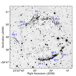
Figure 1: Finding chart for the eight long-slit positions. The background is a [Fe II] 1.644 µm narrow-band image observed in 2008 August. The red cross mark is the expansion center ($\alpha$ = 23^h23^m27^s.77 $\pm$ 0^s.05, $\delta$ = 58^∘48$\arcmin$49$\farcs$4 $\pm$ 0$\farcs$4 [J2000]) of the SN ejecta measured by Thorstensen et al. (2001). Note that the length of each blue bar represents the total effective slit coverage depending on the nodding offset (see Table 1). North is up and east is to the left.

We carried out NIR spectroscopic observations of Cas A using TripleSpec mounted on the Palomar 5 m Hale telescope. TripleSpec is a cross-dispersed NIR spectrograph that provides simultaneous wavelength coverage from 0.94 to 2.46 µm at a spectral resolving power of $R\sim 2700$ (Wilson et al., 2004; Herter et al., 2008). The spectrograph uses two adjacent quadrants, i.e., $2048\times 1024$ pixels, of a Rockwell Scientific Hawaii-II array. The slit width and length are 1″ and 30″, respectively. On 2008 June 29 and August 8, we obtained spectra at eight slit positions along the main ejecta shell (Figure 1). The orientations of Slits 1 and 4 were set perpendicular to the shell, while those of the others were largely parallel to the shell. The nearby A0V star HD223386 was observed as a spectroscopic standard right before and/or after the target observations at similar airmasses. In addition to the target spectra, we also obtained spectra of sky background by dithering along the slit or taking spectra of nearby sky, depending on the complexity of the target fields. The total on-source exposure time at each slit position ranges from 300 to 1800 s. The detailed parameters of the spectroscopic observations are provided in Table 1.

We developed an IDL-based data reduction pipeline to reduce the obtained TripleSpec data. The pipeline first performed subtraction of a dark frame and flat fielding, followed by subtraction of sky background emission. For the latter, we used sky background emission obtained in a dithered frame or in a frame from nearby empty sky, depending on the complexity of the source emission in a given slit. Because of the non-uniform dispersion by the three cross-dispersing prisms in TripleSpec (Wilson et al., 2004; Herter et al., 2008), some orders of the TripleSpec spectra are severely curved. By carefully tracing the spectra of standard stars and airglow emission lines, we obtained a 2D wavelength solution for each order that can correct this effect in a satisfactory manner. We conducted fifth-order order polynomial fits to the wavelengths of the OH airglow emission lines (Osterbrock et al., 1997; Rousselot et al., 2000) in the TripleSpec spectra to obtain the wavelength solutions at 0.5 Å $1\sigma$ uncertainty for each order. Heliocentric velocity correction was also performed when calculating the velocity of the emission line detected in the TripleSpec spectra. We used an A0V-type standard star (HD223386) in the photometric calibration and confirmed that the fluxes of the [Fe II] 1.644 µm emission line are consistent with those from the narrow-band imaging observations of the same areas (see Section 2.2).

2.2 Near-infrared Imaging

In 2005 August 28 and 2008 August 11, we performed NIR imaging observations for the remnant using the Wide-field Infrared Camera (WIRC; Wilson et al., 2003) attached to the Palomar 5 m telescope. The camera consists of a single $2048\times 2048$ Rockwell Hawaii-II HgCdTe NIR detector with a pixel scale of $0\farcs 2487$ pixel^-1, which provides a field of view of $8\farcm 7\times 8\farcm 7$. We used an [Fe II] narrow-band filter that has a mean wavelength of 1.644 µm and a bandwidth of 252 Å. While the single exposure time per frame in 2005 and 2008 is 60 s and 200 s, the multiple dithering observations yield total integration times of 1200 s and 5400 s, respectively. We also obtained H-continuum narrow-band images (mean wavelength of 1.570 µm and bandwidth of 236 Å) in order to subtract the bright stars in the [Fe II] narrow-band images. The average seeing throughout our observations was $\sim 0\farcs 9$ FWHM. We followed standard procedures for the reduction of NIR imaging data. First, the dark and sky background were subtracted from each individual dithered frame. Then, all of the frames were divided by the normalized flat image. The astrometric solution was derived on the basis of unsaturated stars around the remnant in the Two Micron All Sky Survey (2MASS) Point-Source Catalog (PSC; Skrutskie et al., 2006). We coadded all dithered frames which were astrometrically aligned. In terms of photometric calibration, the H-band magnitude in the 2MASS system was used by assuming that the [Fe II] narrow-band magnitude is the same as the H-band magnitude. The uncertainty in the zero-point magnitude we derived is less than 0.1 mag, corresponding to the 10% of the flux.

3 Identification of Knots and Line Parameters

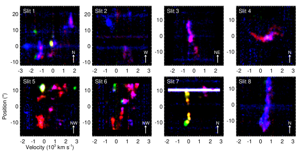
Figure 2: Two-dimensional dispersed image of bright emission lines in three colors: [Fe II] 1.644 µm in red, He I 1.083 µm in green, and [P II] 1.188 µm + [S III] 0.953 µm in blue. The $y$-axis represents the position along the slit length with zero corresponding to the slit center in Table 1. The dynamic ranges of RGB colors are the same, i.e., maximum to minimum intensity ratios of 10, while their maximum intensities have a ratio of 1:10:70 (R:G:B) in each slit image. Note that the continuous spectrum at $+10\arcsec$ in Slit 7 is of an adjacent star falling on the slit position. The slit direction is marked in the lower right of each panel (see Table 1 for details).

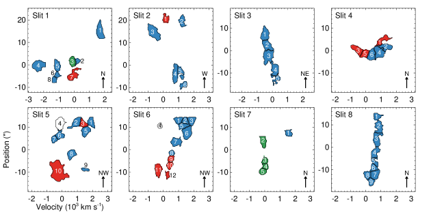
Figure 3: 63 knots identified by the Clumpfind code in the 2D dispersed images. The colors represent the different types of knots: He-rich knots is in green, S-rich knots in blue, and Fe-rich knots in red. Knot 4 in Slits 5 and 6, which are not colored, are composed of two knots of different types with almost the same position and velocity (see Table 2). In Slit 7, there is another knot above Knot 2 (see Figure 2), but it spatially overlaps with a continuum source and was not identified as a clump by the Clumpfind code. The slit direction is marked in the lower right of each panel (see Table 1 for details).

Figure 2 shows 2D dispersed images of strong emission lines detected in our TripleSpec spectra: red for [Fe II] 1.644 µm, green for He I 1.083 µm, and blue for [P II] 1.188 µm + [S III] 0.953 µm. The emission features are complex, often with multiple peaks, and so the identification of individual ‘knots’ by visual inspection is not straightforward. We used the IDL routine Clumpfind (Williams et al., 1994), which was developed for the identification of clumps in molecular clouds. The routine identifies ‘clumps’ by searching for local maxima above some intensity threshold and following them down them to low-intensity levels. For a given 2D dispersed image, a “mask” locating individual knots was generated from [Fe II] 1.644 µm emission features or, if they are weak, [S III] 0.953 µm or [P II] 1.188 µm emission features, and shifted along the wavelength to find other emission lines associated with the knots. The details of this knot identification process are given in the Supplement Material of Koo et al. (2013). In total, we identified 63 knots of distinctive kinematical and spectral properties in the 2D dispersed images. Figure 3 shows their locations and Table 2 lists their positions, sizes, and radial velocities.

We extracted one-dimensional (1D) spectra of individual knots using their mask files (Figure 3). We identified 46 emission lines in total and derived their parameters by performing single Gaussian fits to the detected lines. Table 3 lists the derived line widths and fluxes. [Fe II] 1.644 µm line is detected in all 63 knots and their fluxes are also listed in Table 2. Among the 46 emission lines, 43 lines are previously detected lines in SNRs (Dennefeld & Andrillat, 1981; Rudy et al., 1994; Hurford & Fesen, 1996; Gerardy & Fesen, 2001), whereas three lines of [Fe III] at 2.145, 2.218, and 2.242 µm are detected for the first time in SNRs. The [Fe III] lines originate from transitions between levels in ³G and ³H terms with high excitation energies ($\gtrsim 30{,}000$ K) and have been detected in a few objects, such as SgrA^∗/IRS16 complex (Lutz et al., 1993, and references therein), classical novae (Wagner & Depoy, 1996), H II regions (Okumura et al., 2001), and planetary nebulae (Likkel et al., 2006). Among the previously reported lines, on the other hand, the O I 1.1286, 1.1287 µm, [Fe II] 1.1881 µm, and [Si X] 1.430 µm lines are not detected in our spectra. Gerardy & Fesen (2001) reported detection of the O I lines in the FMKs in Cas A, but we were unable to confirm the detection with our spectra. They also reported detection of the highly ionized [Si X] 1.430 µm line, but again we were unable to confirm the detection. The [Fe II] 1.1881 µm line was included in the list of identified lines in three QSFs in Cas A and the Kepler SNR by Gerardy & Fesen (2001), but we consider that this was a misidentification of the [P II] 1.1883 µm line. The expected flux of the [Fe II] 1.1881 µm line in typical conditions (e.g., $T\lesssim 10^{4}$ K, $n_{\rm e}\lesssim 10^{5}$ cm^-3) in SNRs is almost negligible, i.e., its flux relative to the [Fe II] 1.257 µm line is $\lesssim 10^{-5}$, whereas the [P II] 1.1883 µm line could be as strong as $\sim 1/10$ of the [Fe II] 1.257 µm line for cosmic abundance, or even higher if Fe atoms are locked into dust grains (Koo et al., 2013).

4 Principal Component Analysis of Knots’ Spectral Properties

4.1 Method

In order to systematically characterize the spectral properties of the 63 knots, which have 46 emission lines in total, we applied the PCA method. PCA measures the variances among the original input variables (i.e., brightness of the emission lines in this study) and then sets new orthogonal axes called principal components (PCs) along the largest variances. Therefore, the largest variance (or information) is contained in the first PC (PC1), the second most in PC2, and so forth. If there are significant correlations among the original input variables, then the majority of the information is confined within the first few PCs, which makes it possible to categorize the objects into a few groups based on the first few PCs.

Before performing the PCA, we apply an extinction correction using the line ratio of the [Fe II] 1.257 and 1.644 µm emission. These two lines originate from the same upper level ($a^{4}D_{7/2}$) and therefore their intrinsic flux ratio ($[F_{\rm 1.257}/F_{\rm 1.644}]_{\rm int}$) depends on the Einstein A-coefficients ($A_{\rm ki}$) and their wavelengths, i.e., $[F_{\rm 1.257}/F_{\rm 1.644}]_{\rm int}=(A_{ki,1.257}/1.257)/(A_{ki,1.644}/1.644)$. The A-coefficients, however, are considerably uncertain so the line ratio ranges from 0.98 to 1.49 (Giannini et al., 2015; Koo & Lee, 2015, and references therein) in literature. We adopt a line ratio of 1.36, which is the value suggested by Nussbaumer & Storey (1988) and Deb & Hibbert (2010). (We found that the uncertainty of the theoretical line ratio does not affect our classification of the knots because they are well grouped in PC spaces, as we will show in Section 4.2.1. The criteria of the groups, however, may change depending on the intrinsic line ratio we adopt. In Section 4.2.1, we will describe this in more detail.) Then, by comparing the observed line flux ratio to the intrinsic ratio, we obtain the extinction of the knots and deredden the observed fluxes of all of the lines. We use the general interstellar extinction curve derived from a carbonaceous-silicate grain model with a Milky Way size distribution for $R_{V}=3.1$ (Draine, 2003). The derived extinctions are listed in Table 2. In our previous work (Lee et al., 2015), we showed that the extinction toward the west is systematically larger than that toward the east, which is consistent with the previous optical/X-ray extinction estimates (see Figure 1 in Lee et al., 2015). We further showed that the extinctions of red-shifted knots are systematically higher than those of the blue-shifted knots, implying the presence of a large amount of SN dust inside and around the main ejecta shell (see Lee et al., 2015, for details). The lines from the same upper level in the dereddened spectral data do not provide independent information any more, so that the number of attributes in the PCA are now reduced from 46 to 23. In order to prevent a few bright lines dominating the PCA, the line intensities are standardized by subtracting the mean and dividing by the standard deviation. Since we use the mean-subtracted data, the zero PCs represent the location of mean brightness, not the location of the zero fluxes of the lines (hereafter convergent point), which is important for our classification (see Section 4.2.1). In order to get the PC coefficients of a knot indicating the convergent point when all the emission lines of a knot get close to zero flux, we add one artificial knot into the data set that has emission lines with zero flux.

4.2 Results

4.2.1 Principal Components and Classification of Knots

Table 4 contains the relative and cumulative fraction of variances contributed by the 10 most significant PCs. The first three PCs account for the majority, i.e., $\sim$85%, of the spectral information; thus, we use them in our classification of the knots. Figure 4 shows the projection of the 23 attributes on the combination plane of the three most significant PCs. (This type of plots is known as an h-plot; see Ungerechts et al. (1997) and Neufeld et al. (2007).) While Figure 4(a) and 4(b) show 2D projections on the planes of (PC1 vs. PC2) and (PC1 vs. PC3), Figure 4(c) shows 3D projections for the three PCs together. The lengths of the vectors in the plots are proportional to the fractional contributions by the spectral line to the given PC, and their quadratic sum is equal to unity. In Figure 4(d), we visualize the 3D projections using the coordinate of (Longitude vs. Latitude) representing the two projection angles on the surface of a sphere. We see in Figure 4 that the attributes can be largely divided into three groups, each of which is composed of several strongly correlated spectral lines. (Note that the cosine of the angle between the vectors on the plots measures the linear correlation between the emission lines; see Neufeld et al. (2007) for example.) The first group (hereafter ‘He group’) is composed of H I, He I, and [N I] lines. These lines are almost perfectly correlated with each other. The lengths of their vectors are close to unity in the PC1-PC3 plane, which means that these spectral lines are properly accounted for by PC1 and PC3. The second group (‘S group’) is composed of [Si VI], [P II], and ionized S emission lines. These lines are also strongly correlated with each other and mostly contributed by PC2 and PC3 in the direction orthogonal to the He group lines. The last group (‘Fe group’) is composed of ionized Fe emission lines, i.e., [Fe II] and [Fe III] lines. These lines are rather loosely correlated but are still generally well separated from the lines in the other two groups. The [Fe II] 2.046 and 2.224 µm lines in particular appear somewhat distinct from the other [Fe II] lines. This might be caused by the higher excitation energies of the two lines than those of the other lines, i.e., $\sim 30{,}000$ K vs. $\sim 10{,}000$ K.

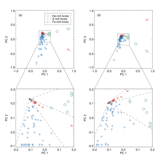
Figure 5: Projections of the 63 objects (or knots) on the plane of (a) PC1-PC2 and (b) PC1-PC3. The green open circles, blue crosses, and red X symbols indicate He-rich, S-rich, and Fe-rich knots, respectively. The enlarged views of the crowded central regions are shown in the lower panels. The black dashed lines in the lower panels represent the criteria of the groups, and the black diamond indicates the convergent point (see text for details). (An interactive 3D pdf version and it source code written in Asymptote are available in a tar.gz package in the electronic journal.)

We plot the PC coefficients of the 63 knots on the PC planes in Figure 5. The central positions of the planes, where (PC1, PC2, PC3) = (0, 0, 0), represent the spectrum made by averaging all of the spectra of all 63 knots. In the lower panels of the figure, which are the enlarged plots of the central areas of the PC planes, we draw dashed lines in order to group the knots (see below) originating from (PC1, PC2, PC3) = (-0.10, 0.23, 0.10). This convergent point is the location of the virtual knot with zero flux (Section 4.1), and the radial distance from the convergent point is proportional to the brightness of the emission line. The distributions of the PC coefficients in Figure 5 are very similar to those in Figure 4. There appear to be three groups of knots in Figure 5 that have PC coefficients similar to those of the three groups in Figure 4, i.e., the He, S, and Fe groups. We therefore group the knots in Figure 5 as He-rich, S-rich, and Fe-rich knots using the dashed lines. As a result, we identify 7 He-rich knots, 45 S-rich knots, and 11 Fe-rich knots.

Figure 6 shows sample 1D spectra of the three groups. As expected, the He-rich knots have strong lines of He I 1.083 µm compared to [Fe II]  and some of them also show several emission lines of H I, [N I], [P II], and [Fe III] as well. The H I and [N I] lines are detected only in the He-rich knots. The S-rich knots also have bright [Fe II] lines, but they have much stronger lines of [S III] 0.953 µm, [S II] 1.03 µm multiplets, [P II] 1.188 µm, and [Si VI] 1.963 µm. The low-ionized emission lines of refractory elements, i.e., [C I] and [Si I], are also detected in several S-rich knots. Although some S-rich knots show the He I 1.083 µm line, their intensities are significantly less than those of the He-rich knots. The Fe-rich knots have strong lines of [Fe II] and some of them have a weak He I 1.083 µm line as well. The brightest Fe-rich knot, Knot 10 in Slit 5, also emits [Fe III] lines in the K band. As in the He-rich knots, no lines of C, Si, and S are detected in the Fe-rich knots.

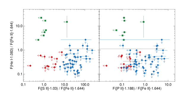
Figure 7: Flux comparisons among the lines of He I (1.083 µm), [S II] (1.03 µm multiplets), and [P II] (1.188 µm). The extinctions are corrected and the fluxes are normalized by the [Fe II] 1.644 µm line fluxes. The three knot groups are represented by green squares (He-rich knots), blue circles (S-rich knots), and red diamonds (Fe-rich knots). The arrows represent $3\sigma$ upper limits.

The three knot groups are easily distinguishable when the flux ratios of [S II] 1.03 µm multiplets, He I 1.083 µm, and [P II] 1.188 µm are compared (Figure 7). The He-rich knots are well separated from the other groups in F(He I-1.083)/F([Fe II]-1.644), i.e., the ratio is greater than two for the He-rich knots but lower than two for the S-rich and Fe-rich knots. The F([S II]-1.03)/F([Fe II]-1.644) and F([P II]-1.188)/F([Fe II]-1.644) of the He-rich knots are mostly smaller than a few times 1.0 and 0.1, respectively. Although the S-rich and Fe-rich knots are not clearly distinguished in the F([S II]-1.03)/F([Fe II]-1.644) and F([P II]-1.188)/F([Fe II]-1.644) comparisons, we see that these ratios are higher in the S-rich knots than the Fe-rich knots, i.e., F([S II]-1.03)/F([Fe II]-1.644) $\gtrsim 5$ and F([P II]-1.188)/F([Fe II]-1.644) $\gtrsim 0.3$ for the S-rich knots and vice versa. It is worth noting that the flux ratios of the knots in Figure 7 and the criteria mentioned above are based on the assumption that the intrinsic flux ratio of [Fe II] 1.257 and 1.644 µm is 1.36 (Section 4.1). If we adopt different line ratios, e.g., 0.98 to 1.49 (Giannini et al., 2015; Koo & Lee, 2015, and references therein), then the criteria of those three flux ratios will be F(He I-1.083)/F([Fe II]-1.644) = 1.0–2.4, F([S II]-1.03)/F([Fe II]-1.644) = 2.3–6.0, and F([P II]-1.188)/F([Fe II]-1.644) = 0.19–0.34.

4.2.2 Physical Properties of Three Knot Groups

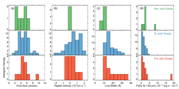
Figure 8: Histograms of (a) knot size, (b) radial velocity, (c) line width, and (d) extinction-corrected [Fe II] 1.644 µm flux.

Figure 8 compares the distributions of the knot sizes, radial velocities, and line widths of the three knot groups. The angular sizes of most of the knots are in the range 2″–7″ (or 0.03–0.1 pc at a distance of 3.4 kpc) and there is no significant difference among the three groups in their sizes, although some of the S-rich and Fe-rich knots are as large as 10″. On the other hand, there are significant differences in their radial velocities and line widths. The radial speeds of He-rich knots are $\lesssim 200~{}{\rm km~{}s}^{-1}$, while those of S-rich knots range from $-2000~{}{\rm km~{}s}^{-1}$ to $+2000~{}{\rm km~{}s}^{-1}$ with a median of $+630~{}{\rm km~{}s}^{-1}$. The radial velocities of Fe-rich knots range from $-500~{}{\rm km~{}s}^{-1}$ to $+1500~{}{\rm km~{}s}^{-1}$ with a median of $+330~{}{\rm km~{}s}^{-1}$. In line width, the He-rich knots have widths of 5–10 Å, while the S- and Fe-rich knots have widths of 10–35 Å. (Note that our spectral resolution at 1.64 µm is $\sim 6$ Å.) Figure 8 also compares the distribution of the [Fe II] 1.644 µm line fluxes among the three knot groups. While the S-rich and Fe-rich knots have a similar distribution with an increased number of knots that have faint [Fe II] emission, the pattern is absent in the He-rich knots. There is no apparent correlation among the four physical parameters of the knots.

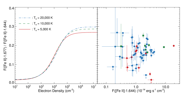
Figure 9: (Left) F([Fe II]-1.677)/F([Fe II]-1.644) ratio as a function of electron density for gas in statistical equilibrium at $T_{e}=$ 5000 K, 10,000 K, and 20,000 K. (Right) F([Fe II]-1.677)/F([Fe II]-1.644) vs. F([Fe II]-1.644) of the knots. The symbols are the same as in Figure 7. All fluxes are extinction-corrected.

One of the physical parameters of the knots that can be straightforwardly obtained is electron density using [Fe II] lines originating from levels with similar excitation energies, because their ratios are mainly determined by electron densities (e.g., Koo et al., 2016). [Fe II] 1.644 µm and 1.677 µm are such lines, and Figure 9 compares their expected ratios as a function of density for the assumed temperatures of 5000, 10,000, and 20,000 K (left panel) with observed values as a function of the [Fe II] 1.644 µm flux (right panel). We see that the ratio is quite insensitive to temperature and can be used to estimate electron density in the range $\sim 10^{3}$–$10^{5}~{}{\rm cm^{-3}}$. The electron density of the He-rich knots is a few $10^{4}~{}{\rm cm^{-3}}$, while the S-rich knots show electron densities over a broad range of $10^{3}~{}{\rm cm^{-3}}$ to $10^{5}~{}{\rm cm^{-3}}$. The Fe-rich knots have somewhat lower ($10^{3}$–$10^{4}~{}{\rm cm^{-3}}$) electron densities compared to the other two groups. There appears to be no correlation between the electron densities and [Fe II] 1.644 µm line fluxes.

5 Discussion

In this section, we discuss the origin of the knots using their spectral characteristics described in the previous section.

5.1 He-rich and S-rich knots

The He-rich and S-rich knots have quite distinct spectral properties; the He-rich knots have high F(He I-1.083)/F([Fe II]-1.644) and low F([S II]-1.03)/F([Fe II]-1.644), F([P II]-1.188)/F([Fe II]-1.644), while the S-rich knots have low F(He I-1.083)/F([Fe II]-1.644) and high F([S II]-1.03)/F([Fe II]-1.644), F([P II]-1.188)/F([Fe II]-1.644). Their kinematic properties are also quite different; the He-rich knots have low ($\lesssim 200~{}{\rm km~{}s}^{-1}$) line-of-sight speeds, while the S-rich knots have high (up to $\sim 2000~{}{\rm km~{}s}^{-1}$) line-of-sight speeds. These spectral and kinematical properties suggest that the He-rich knots are dense, slow-moving CSM swept up by the SN blast wave, while the S-rich knots are fast-moving SN ejecta that have been shocked. The same conclusion was reached by Koo et al. (2013), who performed an abundance analysis using [P II] 1.188 µm and [Fe II] 1.257 µm lines. They showed that the relative abundance of P (a major product of the stellar Ne-burning layer) to Fe (in number) for the He-rich knots is similar to the solar abundance, whereas that of the S-rich knots is 10–100 times higher than the solar abundance.

The characteristics of the two types of knots match well with those of QSFs and FMKs known from previous optical studies (see Section 1 for a summary of their properties). Similar to the optical QSFs, the He-rich knots have bright He I lines together with H I and [N I] lines; all the He-rich knots have a He I 1.083 µm line, 6 out of the 7 show H I Pa$\beta$, Br$\gamma$ lines, and the three brightest ones also have [N I] 1.040, 1.041 µm lines. Like the optical FMKs dominated by lines of ionized heavy elements O, S, Ar, the S-rich knots show strong S lines plus [P II] and [Si VI] lines; all the S-rich knots have [S II] 1.03 µm multiplets, and 39 out of 45 S-rich knots also have [P II] 1.188 µm and/or [Si VI] 1.963 µm lines. Indeed, the overall spectra of He-rich and S-rich knots are similar to the NIR spectra of QSFs and FMKs obtained by Gerardy & Fesen (2001), respectively. Furthermore, the radial velocities of the two NIR knot groups are well consistent with those of the optical groups. For example, the radial velocity of the He-rich knots is $-50\pm 90~{}{\rm km~{}s}^{-1}$, while the generally accepted radial velocity of QSFs is $-140\pm 300~{}{\rm km~{}s}^{-1}$ (van den Bergh & Kamper, 1985; Reed et al., 1995). In addition, the median line-of-sight velocity of S-rich knots is $+620~{}{\rm km~{}s}^{-1}$, while the systematic velocity of the FMKs is $+770\pm 40~{}{\rm km~{}s}^{-1}$ (Reed et al., 1995).

Rich emission lines of Si, P, and S in the S-rich knots and FMKs imply that they are the SN ejecta originated from the Ne- and O-burning layers. The two bright emission lines, [P II] 1.188 µm and [Fe II] 1.644 µm, have comparable excitation energies and critical densities, and so their line ratios are strongly dependent on their abundance ratio, $X$(P/Fe) (Koo et al., 2013). As seen in Figure 7, there is a large scatter in this line ratio for S-rich knots, which implies that the abundance ratio $X$(P/Fe) varies almost two orders of magnitude for these knots. We also found that 13 out of 45 S-rich knots have clear but relatively weak emission lines of He I and/or [C I]. The detection of the He, C, and Fe lines in the S-rich ejecta, which are either lighter or heavier elements than the O-burning materials, might infer microscopic mixing during the SN explosion. In many S-rich knots, a highly ionized Si line, [Si VI] 1.963 µm, is detected, while in a few S-rich knots, a [Si I] 1.645 µm line is also detected. The detection of Si in very different ionization stages indicates the broad range of temperatures in the S-rich knots.

5.2 Fe-rich knots

In Section 4.2, we found that the Fe-rich knots exhibit intermediate characteristics between He-rich and S-rich knots; they emit strong [Fe II] lines without any Si, P, and S lines, but have high line-of-sight speeds of up to $\sim 1500~{}{\rm km~{}s}^{-1}$. A few knots also emit an He I 1.083 µm line. The high velocities, however, suggest that they are not dense QSFs represented by the He-rich knots. Their line widths are also considerably broader than those of He-rich knots, i.e., 10–35 Å vs. 5–10 Å (Figure 8). On the other hand, the missing Si, P, and S lines indicate that the abundances of these Ne- and O-burning elements are very low in these Fe-rich knots. We can consider two possible explanations regarding the origin of the Fe-rich knots: (1) swept-up CSM around contact discontinuity (CD) or (2) shocked SN ejecta enriched with Fe elements that had been synthesized in explosive Si burning. The ambient medium that the Cas A SN blast wave is propagating into is believed to be CSM with an $r^{-2}$ density distribution (e.g., Lee et al., 2014). In such a case, 1D similarity solutions show that the shocked CSM accumulates at the CD with infinite density asymptotically (Chevalier, 1982). We thus expect “dense” CSM expanding at a speed comparable to the shocked SN material. In the real situation, however, this interacting region between the shocked SN ejecta and the shocked CSM is hydrodynamically unstable and distorted, with the density of the shocked CSM limited to $\lesssim 10$ times the density at the ambient shock (Chevalier et al., 1992; Blondin et al., 2001; van Veelen et al., 2009). The temperature of the shocked CSM near the CD, therefore, may be lower than the typical temperature ($\sim 2$ keV) of the shocked CSM (Hwang & Laming, 2012), but probably no more than a factor of 10, and all of the Fe in the shocked CSM will be in high ionization stages. Furthermore, H I lines are not detected in all Fe-rich knots with an upper limit of F(H I-Pa$\beta$)/F([Fe II]-1.257) $\lesssim 0.1$. Note that the observed ratio of these line intensities ranges between 0.05 and 10 for SNRs while it is $\sim 50$ for Orion, which should be the typical ratios for shocked and photoionized gases of cosmic abundance, respectively (Koo & Lee, 2015). Therefore, H must be depleted in Fe-rich knots. The non-detection of He and N lines might also indicate that the abundances of these ‘circumstellar’ elements are very low in Fe-rich knots, although this needs to be confirmed from other waveband observations. (See the next paragraph for an explanation of the faint He lines detected in some Fe-rich knots.) We may therefore conclude that the Fe-rich knots are not likely the shocked CSM.

This leaves the second possibility, i.e., the Fe-rich knots are Fe-enriched SN ejecta. The high velocities and large velocity widths are consistent with SN ejecta being swept up by the reverse shock. The low [P II] and [S II] fluxes compared to the [Fe II] flux, however, implies that the abundances of P and S, which are Ne- and O-burning materials, are very low, which is in sharp contrast to the S-rich knots. These characteristics strongly suggest that the Fe-rich knots are most likely “pure” Fe ejecta synthesized in the deepest stellar interior. The weak He I 1.083 µm line detected in some Fe-rich knots could be due to an $\alpha$-rich freeze-out process during the explosive Si burning; just after the explosion, complete Si burning with an $\alpha$-rich freeze-out occurs under high temperatures and low density conditions in the stellar deep layer, and many alpha particles are “frozen out” without participating in further nucleosynthetic processes (Woosley et al., 1973). Similar dense, Fe-predominant ejecta, likely from the $\alpha$-rich freeze-out process, have been detected in another young core-collapse SNR G11.2-0.3 (Moon et al., 2009).

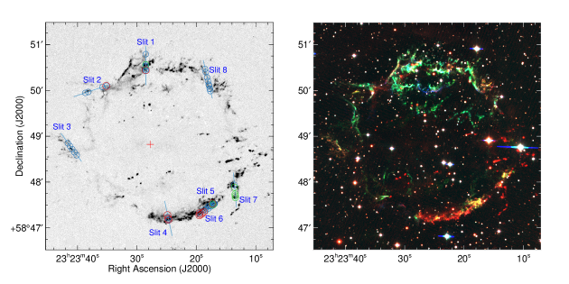
Figure 10: (Left) Locations of 63 knots in Table 2. (See Figure 3 for the knot numbers in each slit.) The He-rich, S-rich, and Fe-rich knots are marked in green, blue, and red, respectively. The background is the continuum-subtracted [Fe II] 1.644 µm narrow-band image in Figure 1. (Right) A three-color composite image of Cas A with an [Fe II] 1.644 µm narrow-band image in red, and HST ACS/WFC F850LP and F775W images in green and blue. The HST images are dominated by [S III] 9069, 9531 Å and [S II] 1.03 µm multiplets (F850LP) and [O II] 7319, 7330 Å lines (F775W), respectively (Fesen et al., 2006; Hammell & Fesen, 2008). The [Fe II] 1.644 µm image was observed in 2005 August. The HST ACS/WFC images are from the Hubble Legacy Archive (https://hla.stsci.edu) and they were taken in 2004 December (Fesen et al., 2006). To match their angular resolutions, the HST images were smoothed by using a Gaussian kernel with a FWHM of 0$\farcs$9.

Pure Fe ejecta have been detected in X-rays (see below) but not in optical or NIR wavebands. This is surprising considering the extensive optical/NIR studies carried out for Cas A since its discovery. Figure 10 partly gives an answer. In the right panel of Figure 10, red is an [Fe II] 1.644 µm narrow-band image while green and blue are Hubble Space Telescope (HST) ACS/WFC F850LP and F775W images which are dominated by ionized S and O lines, respectively (Fesen et al., 2006; Hammell & Fesen, 2008). Previous optical observations had been mostly toward the northern ejecta shell bright in ionized O, S, and Ar lines (e.g., Chevalier & Kirshner, 1979; Hurford & Fesen, 1996; Fesen et al., 2001) or toward FMKs outside the main shell (e.g., Fesen et al., 1988, 2006; Fesen, 2001). Figure 10, however, shows that the southwestern (SW) main ejecta shell, which is bright in the [Fe II] line but faint in the ionized O and S lines, is the region where Fe-rich ejecta can be found. Indeed, our result shown in the left panel of Figure 10 confirms this; 9 out of 11 Fe-rich knots are located in Slits 4–6. (Note that the compact red knots in the interior and beyond the SW shell are mostly QSFs, and they are bright in [N II] 6548, 6583 Å and H$\alpha$ images too (van den Bergh & Kamper, 1985; Alarie et al., 2014).) The slit positions are determined from an [Fe II] 1.644 µm image, so that some of them were placed toward the red portions of the main ejecta shell and, by decomposing the emission into individual velocity components, we were able to identify Fe-rich ejecta. It is worth noting that Rho et al. (2003) also noted the bright [Fe II] emission in the SW shell in their [Fe II] 1.644 µm image of Cas A. Meanwhile, we can see that the [Fe II] 17.9 µm emission is much brighter than the emission from O-burning elements such as Ar and S in the SW shell in the Spitzer mid-infrared maps of ionic lines (Ennis et al., 2006; Smith et al., 2009). Our result suggests that this [Fe II] emission-predominant area, i.e., the red area of the SW ejecta shell in Figure 10, is probably mainly composed of Fe ejecta.

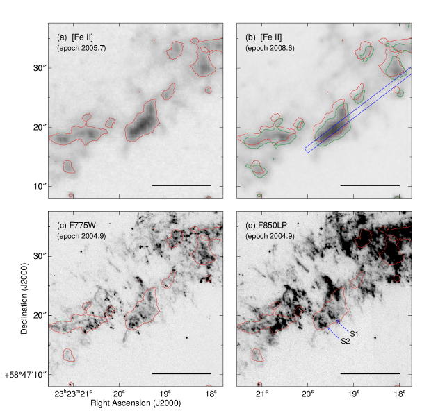
Figure 11: Enlarged views of the SW shell where the brightest Fe-rich knot (Knot 10 in Slit 5; K10) has been detected. (a)–(b) [Fe II] 1.644 µm narrow-band images obtained in 2005 August and in 2008 August. The red and green contours indicate the brightness level of $1\times 10^{-4}~{}{\rm erg}~{}{\rm s}^{-1}~{}{\rm cm}^{-2}~{}{\rm sr}^{-1}$ in the 2005 and 2008 images, respectively. The blue bar in the 2008 image represents the position of Slit 5 across Knot 10. (c)–(d) HST ACS/WFC F775W and F850LP images taken in 2004 December. The red contours overlaid on the images are the same as in (a). (d) S1 and S2 are the two bright knots mentioned in Section 5.2. The angular resolutions are 0$\farcs$1 and 0$\farcs$9 for the optical and [Fe II] images, respectively. The black scale bar in the lower right of each panel represents an angular scale of 10″, and the low and high thresholds of the grayscale are $-5\times 10^{-5}$ and $5\times 10^{-4}~{}{\rm erg}~{}{\rm s}^{-1}~{}{\rm cm}^{-2}~{}{\rm sr}^{-1}$ in all images.

It is not easy to identify the counterpart of Fe-rich knots in optical images because several velocity components are usually superposed along the line of sight toward the main ejecta shell. The brightest Fe-rich knot (Knot 10 in Slit 5; hereafter K10), however, is somewhat isolated and we can identify its counterpart. In Figure 11, the upper two images are [Fe II] 1.644 µm images at different epochs and they show that K10 is a clump of $\sim 10\arcsec\times 3\arcsec$ elongated along the slit. The two [Fe II] images clearly show that the clump is moving fast tangentially. The proper motion is measured $0\farcs 28$ yr^-1, implying a tangential velocity of $4500\pm 200~{}{\rm km~{}s}^{-1}$. In the lower F775W and F850LP images, we see diffuse faint emission at the position of K10 (see the red contour). Its brightness distribution is different, with two small ($\lesssim 2\arcsec$) bright spots (S1 and S2 in the figure) in the lower part of the clump. One of these bright spots, S1, is coincident with an S-rich knot (Knot 9 in Slit 5), which is spatially coincident with K10 but has a line-of-sight velocity ($+1500~{}{\rm km~{}s}^{-1}$) that is very different from that of K10 ($-300~{}{\rm km~{}s}^{-1}$). The other bright spot, S2, must also be due to an S-rich knot not detected in our spectroscopy. So excluding these two bright knots, K10 appears faint in F775W and F850LP images. We suspect that most of the diffuse emission in the F775W and F850LP images is due to optical [Fe II] lines. This can be confirmed by optical spectroscopy. Recently, there have been optical spectral mapping observations of Cas A (Reed et al., 1995; Milisavljevic & Fesen, 2013; Alarie et al., 2014) and, in principle, a similar analysis can be done to detect Fe-rich knots, although the optical [Fe II] lines, e.g., [Fe II] 7155 and 8617 Å lines, will be much fainter than the [Fe II] 1.644 µm line because of large interstellar extinction ($A_{\rm V}=5$–10 mag) toward Cas A (e.g., Eriksen et al., 2009; Hwang & Laming, 2012; Lee et al., 2015).

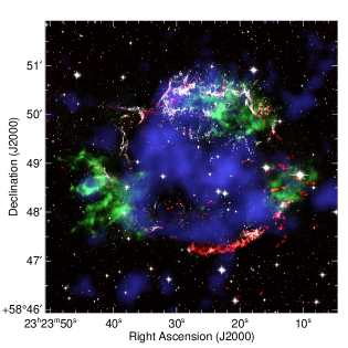
Figure 12: A four-color composite image of Cas A with the [Fe II] 1.644 µm narrow-band image in Figure 1 in red, the Chandra Fe K-shell (6.52–6.94 keV) image in green (Hwang et al., 2004), the NuSTAR hard X-ray ⁴⁴Ti (67.9 and 78.4 keV) image in blue (Grefenstette et al., 2014), and the HST ACS/WFC F850LP image in white (Fesen et al., 2006).

The distribution and amount of Fe ejecta in Cas A have been a subject of controversy. Previous X-ray studies detected hot and diffuse “pure” Fe ejecta with mass $\sim 0.1~{}M_{\sun}$ that might have formed by $\alpha$-rich freeze-out during the complete Si burning (Hwang & Laming, 2003, 2012). These X-ray-emitting shocked Fe ejecta are distributed mainly in the southeastern and northern regions of the remnant (Figure 12). On the other hand, the hard X-ray emission from the radioactive decay of ⁴⁴Ti has been detected in the interior of the main ejecta shell (Figure 12; Grefenstette et al., 2014). Since ⁴⁴Ti is essentially synthesized in complete Si burning with $\alpha$-rich freeze-out in the innermost region (e.g., Magkotsios et al., 2010), ⁴⁴Ti traces “pure” ⁵⁶Ni or its stable nuclei ⁵⁶Fe. The majority of the observed ⁴⁴Ti is inside the reverse shock and therefore from unshocked Fe ejecta. The inferred mass of the unshocked Fe ejecta is $\sim 0.1~{}M_{\sun}$ (Grefenstette et al., 2014). Such unshocked Fe ejecta, however, have not yet been detected, presumably because they are cool ($T\lesssim 40$ K; e.g., Barlow et al., 2010; Sibthorpe et al., 2010; Lee et al., 2015). Instead, the X-ray-emitting Fe ejecta located just outside the ⁴⁴Ti emission was attributed to the corresponding shocked ejecta (Figure 12; Grefenstette et al., 2014). However, the missing X-ray-emitting Fe ejecta toward the south and northeast directions from the explosion center have been puzzling. We note that the NIR [Fe II]-bright, red portion of the SW shell appears to be in contact with the interior ⁴⁴Ti-emitting region (Figure 12). This might be the case for the small red portion near Slit 2 in the northeastern shell, too. Therefore, if these [Fe II]-bright regions are composed of shocked, dense Fe ejecta, as implied from our spectroscopic result, it explains why we do not see X-ray-emitting diffuse Fe ejecta toward these directions; the unshocked “pure” Fe ejecta traced by the radioactive ⁴⁴Ti emission in the interior of the main shell is composed of both dense and diffuse ejecta, and when these are swept up by a reverse shock, we observe either NIR [Fe II] emission or X-ray emission depending on their densities. We do not see NIR emission associated with the central bright ⁴⁴Ti emission but this could be because the shock is face-on, as suggested by the large red-shifted central velocity (1100–3000 ${\rm km~{}s}^{-1}$) of the ⁴⁴Ti line (Grefenstette et al., 2014), or because the reverse shock has not yet reached the dense, unshocked Fe ejecta. Recent multi-dimensional simulations show that such global asymmetry in Fe (or ⁵⁶Ni) density can arise from the low-mode convection of the innermost region just after the core bounce (e.g., Wongwathanarat et al., 2013). Future NIR spectral mapping observations revealing the 3D distribution of the dense Fe ejecta will be helpful for understanding the SN explosion dynamics of the innermost region.

6 Summary

We have carried out NIR spectroscopic observations toward the main ejecta shell of the young SNR Cas A. In total, 63 individual knots were identified from eight slit positions by using a clump-finding algorithm. Each of these knots has distinct kinematical and spectral properties. Within the JHK spectral range (0.94–2.46 µm), we found 46 emission line features including a dozen bright [Fe II] lines, forbidden lines of other metallic species, and H and He lines. We employed the PCA method to classify the knots based on their relative line fluxes into three distinctive groups: He-rich knots of pre-supernova circumstellar wind material, plus S-rich and Fe-rich knots of SN ejecta material. The He-rich and S-rich knots correspond to QSFs and FMKs studied in the visible waveband, while Fe-rich knots, showing in general only [Fe II] emission lines, are likely ‘pure’ dense Fe ejecta from the innermost layer of the progenitor. We summarize our main results as follows.

1. The PCA showed that the NIR spectral lines can be grouped into three groups: (1) Group 1, composed of H I and He I lines together with [N I] lines, (2) Group 2, composed of forbidden lines of Si, P, and S, and (3) Group 3, composed of forbidden Fe lines. The lines in the first two PCs are strongly correlated with each other, while the correlation is rather weak among the forbidden Fe lines in Group 3. These three spectral groups of the emission lines are almost independent in 3D PC space (Figure 4).

2. The distribution of the knots in the PC planes matches well with the above spectral groups, and we classified the knots into three groups: (1) He-rich, (2) S-rich, and (3) Fe-rich knots. The knots belonging to these three groups are well separated from each other in F([S II]-1.03)/F([Fe II]-1.644) vs. F(He I-1.083)/F([Fe II]-1.644) plane (Figure 7), so that one may use these line ratios to classify the knots in Cas A. It would be interesting to determine whether this classification methodology applies for other core-collapse SNRs.

3. The He-rich knots show bright emission lines of He I 1.083 µm and [Fe II] together with [N I] and H I lines. Their line-of-sight speeds are small ($\lesssim 200~{}{\rm km~{}s}^{-1}$). From these chemical and kinematical characteristics, we conclude that the He-rich knots are dense CSM swept up by the SN blast wave. These knots correspond to the previously known QSFs.

4. The S-rich knots show strong forbidden lines of S together with [P II] and [Si VI], and their line-of-sight speeds reach a few 1000 ${\rm km~{}s}^{-1}$. These chemical and kinematical properties indicate that the S-rich knots are dense SN ejecta material mostly originating from the O-burning layers and swept up by a reverse shock. These knots correspond to the FMKs detected in previous optical studies.

5. The Fe-rich knots only show strong [Fe II] and [Fe III] lines, and no or weak He I 1.083 µm lines. Like the S-rich knots, they have large line-of-sight speeds (up to $\sim 1500~{}{\rm km~{}s}^{-1}$) and broad line widths (10–35 Å), but they do not show the lines from Si, P, and S. Some Fe-rich knots show He I 1.083 µm  but their fluxes compared to the [Fe II] lines are much weaker than those of the He-rich knots. These spectroscopic properties suggest that the Fe-rich knots are most likely “pure” dense Fe ejecta from the innermost layer of the SN. The comparison of [Fe II] 1.644 µm images with the HST ACS/WFC F850LP and F775W and NuSTAR ⁴⁴Ti images reveals that these Fe ejecta are mainly distributed in the SW main ejecta shell, just outside the unshocked ⁴⁴Ti in the interior. This supports that there could be a large amount of unshocked “pure” Fe ejecta associated with ⁴⁴Ti. Together with the diffuse, X-ray-emitting “pure” Fe ejecta detected by Chandra, our result implies that the Fe ejecta synthesized in the innermost region develop large-scale non-uniformity during the SN explosion and are expelled asymmetrically. This seems to be consistent with the low-mode, convection-driven SN explosion model.

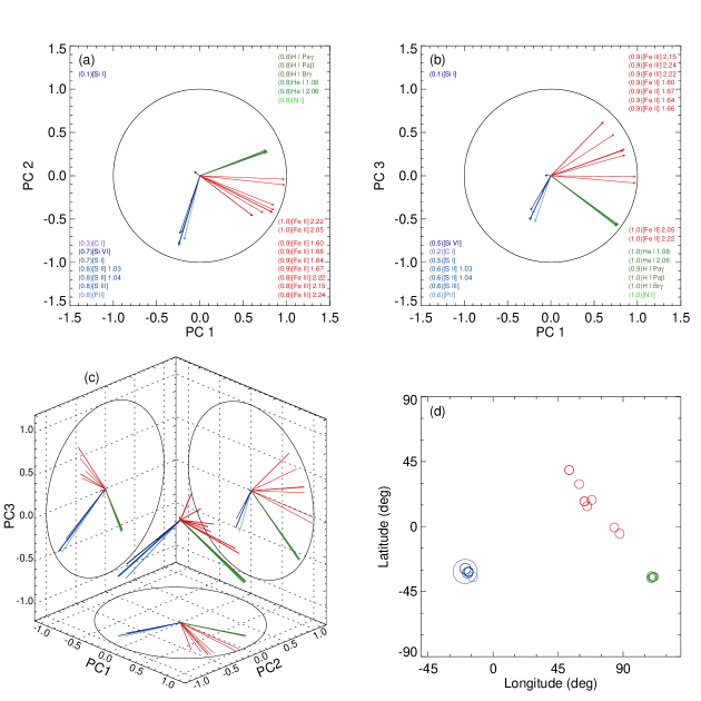
Figure 4: Projections of the 23 attributes (or spectral lines) on the plane of (a) PC1-PC2 and (b) PC1-PC3. A circle of unity radius is overplotted for comparison. The number within parentheses at the corners of (a) and (b) is radius from the center, that represents the normalized contribution of the line at each PC plane. The 3D projections and the projections within a sphere are in (c) and (d), respectively (see the text for details). The reference position in (d), where (Longitude, Latitude) = (0°, 0°), corresponds to (PC1, PC2, PC3) = (0, -1, 0), and Longitude and Latitude are measured toward east and north, respectively. The size of circles in (d) is inversely proportional to the length of the vector in (c). (An interactive 3D pdf version and it source code written in Asymptote are available in a tar.gz package in the electronic journal.)

Figure 6: Sample 1D spectra of He-rich (Knot 5 in Slit 7), S-rich (Knot 3 in Slit 3), and Fe-rich (Knot 10 in Slit 5) knots. The spectra have been smoothed by a Gaussian kernel with an FWHM of 1 pixel (2–3 Å).

Table 1: Parameters of the Spectroscopic Observations

Date	Slit	Central Coordinate	P.A.	Mode	Slit Length	Exposure
(UT)		$\alpha$(J2000)       $\delta$(J2000)	(deg)		(″)	(s)
2008 Jun 29	1	23:23:28.54 +58:50:32.2	0.0	Both	50.50	300 $\times$ 4
	8	23:23:18.13 +58:50:14.4	13.4	AB	51.00	300 $\times$ 5
	2	23:23:37.60 +58:49:59.7	288.7	AB	50.25	300 $\times$ 4
	ST	23:48:53.97 +59:58:44.3	0.0	AB	30.00	30 $\times$ 6
2008 Aug 08	3	23:23:41.11 +58:48:45.2	36.1	AB	45.25	300 $\times$ 6
	4	23:23:24.77 +58:47:12.2	12.0	AB	46.25	300 $\times$ 6
	5	23:23:18.50 +58:47:25.1	307.3	OS	30.00	300 $\times$ 1
	6	23:23:18.33 +58:47:23.5	307.3	OS	30.00	300 $\times$ 1
	7	23:23:13.57 +58:47:49.2	5.2	AB	45.25	300 $\times$ 6
	ST	23:48:53.97 +59:58:44.3	0.0	AB	30.00	30 $\times$ 8

Table 2: Physical Parameters of 63 Identified Knots

Slit	Knot	Central Position	Size	Knot	$A_{\rm V}$	$v_{\rm rad}$	[Fe II] 1.644 µm Flux
No.	No.	$\alpha$(J2000)   $\delta$(J2000)	(″)	Type	(mag)	(${\rm km~{}s}^{-1}$)	(10-17 erg s-1 cm-2)
1	1	23:23:28.54   +58:50:47.6	8.75	S	8.0 (0.5)	$+1698$ ( 2)	589 ( 8)
1	2	23:23:28.54   +58:50:34.1	3.25	S	10.6 (0.7)	$+225$ ( 2)	165 ( 4)
1	3	23:23:28.54   +58:50:33.8	5.00	He	5.8 (0.1)	$-75$ ( 2)	793 ( 5)
1	4	23:23:28.54   +58:50:32.3	5.50	S	3.3 (2.0)	$-2234$ (17)	96 (13)
1	5	23:23:28.54   +58:50:31.1	5.75	S	4.9 (0.2)	$-1083$ ( 2)	383 ( 3)
1	6	23:23:28.54   +58:50:27.6	3.00	S	3.3 (0.5)	$-1091$ ( 3)	132 ( 4)
1	7	23:23:28.54   +58:50:26.6	5.75	Fe	9.8 (0.4)	$-17$ ( 2)	561 (10)
1	8	23:23:28.54   +58:50:25.8	3.00	S	3.4 (0.4)	$-1264$ ( 2)	198 ( 5)
2	1	23:23:35.19   +58:50:06.0	4.50	Fe	5.5 (0.9)	$+185$ ( 6)	204 (10)
2	2	23:23:35.10   +58:50:06.3	5.75	S	9.3 (3.6)	$+1271$ (14)	75 (10)
2	3	23:23:35.83   +58:50:04.3	8.00	S	4.2 (1.7)	$-653$ (20)	140 (12)
2	4	23:23:38.21   +58:49:58.1	9.25	S	7.0 (0.5)	$+814$ ( 3)	480 (10)
2	5	23:23:38.21   +58:49:58.1	6.50	S	11.0 (1.0)	$+1124$ ( 3)	339 (12)
2	6	23:23:38.70   +58:49:56.8	3.75	S	9.2 (1.7)	$+1337$ ( 2)	164 ( 7)
3	1	23:23:41.64   +58:48:50.9	6.75	S	8.2 (0.3)	$-473$ ( 3)	460 ( 6)
3	2	23:23:41.28   +58:48:47.0	5.00	S	7.6 (0.3)	$-397$ ( 3)	310 ( 4)
3	3	23:23:40.92   +58:48:43.2	7.25	S	7.3 (0.1)	$-297$ ( 2)	972 ( 4)
3	4	23:23:40.52   +58:48:38.9	6.50	S	7.2 (0.3)	$+222$ ( 4)	434 ( 8)
3	5	23:23:40.16   +58:48:35.1	5.75	S	6.2 (1.2)	$+341$ ( 7)	121 ( 7)
4	1	23:23:24.90   +58:47:16.8	5.25	Fe	15.4 (1.4)	$+1109$ ( 5)	240 ( 6)
4	2	23:23:24.82   +58:47:13.9	3.75	S	10.6 (0.6)	$+1306$ ( 4)	289 ( 4)
4	3	23:23:24.77   +58:47:12.2	5.75	Fe	7.5 (0.4)	$-491$ ( 3)	298 ( 5)
4	4	23:23:24.73   +58:47:10.7	6.25	S	9.9 (0.3)	$+907$ ( 3)	606 ( 5)
4	5	23:23:24.73   +58:47:10.7	4.00	Fe	6.6 (0.4)	$-31$ ( 4)	236 ( 4)
4	6	23:23:24.72   +58:47:10.2	5.75	S	10.3 (0.3)	$+390$ ( 3)	577 ( 6)
5	1	23:23:17.21   +58:47:32.7	5.25	S	11.5 (0.8)	$+1924$ ( 3)	313 ( 7)
5	2	23:23:17.28   +58:47:32.3	5.25	S	8.8 (0.5)	$+992$ ( 3)	561 (10)
5	3	23:23:17.34   +58:47:32.0	4.50	Fe	8.7 (0.9)	$+1388$ ( 4)	286 ( 8)
5	4A	23:23:17.26   +58:47:32.4	6.25	S	8.3 (0.3)	$-109$ ( 3)	537 ( 7)
5	4B	23:23:17.34   +58:47:32.0	6.25	He	8.3 (0.1)	$-109$ ( 3)	2149 ( 7)
5	5	23:23:17.62   +58:47:30.3	5.25	S	9.3 (0.5)	$+1550$ ( 3)	456 ( 6)
5	6	23:23:17.88   +58:47:28.8	4.75	S	8.8 (0.8)	$-177$ ( 4)	273 ( 8)
5	7	23:23:18.00   +58:47:28.0	3.75	S	7.2 (0.6)	$-492$ ( 3)	215 ( 5)
5	8	23:23:18.72   +58:47:23.8	5.00	S	10.8 (0.5)	$+624$ ( 3)	492 ( 9)
5	9	23:23:19.41   +58:47:19.7	1.75	S	11.9 (1.8)	$+1530$ ( 8)	99 ( 5)
5	10	23:23:19.49   +58:47:19.3	9.75	Fe	7.9 (0.0)	$-290$ ( 3)	4959 ( 8)
6	1	23:23:17.02   +58:47:31.3	3.50	S	6.6 (0.9)	$+1000$ ( 6)	245 ( 8)
6	2	23:23:17.07   +58:47:31.0	3.25	S	9.0 (0.7)	$+1412$ ( 4)	340 ( 7)
6	3	23:23:16.94   +58:47:31.7	4.25	S	10.2 (0.3)	$+1914$ ( 3)	667 ( 7)
6	4A	23:23:17.22   +58:47:30.0	2.75	He	10.0 (2.1)	$-166$ ( 6)	58 ( 6)
6	4B	23:23:17.30   +58:47:29.6	2.75	S	10.4 (3.6)	$-166$ ( 6)	34 ( 6)
6	5	23:23:17.22   +58:47:30.0	3.00	S	7.4 (0.8)	$+1343$ ( 5)	272 ( 6)
6	6	23:23:17.53   +58:47:28.2	6.25	S	10.4 (0.4)	$+1547$ ( 3)	714 ( 8)
6	7	23:23:17.99   +58:47:25.5	4.50	S	7.8 (0.3)	$+802$ ( 3)	623 ( 8)
6	8	23:23:18.47   +58:47:22.6	2.75	S	9.3 (0.7)	$+572$ ( 4)	171 ( 5)
6	9	23:23:18.75   +58:47:21.0	2.75	Fe	8.3 (0.5)	$+540$ ( 4)	258 ( 5)
6	10	23:23:19.04   +58:47:19.3	3.50	Fe	7.3 (0.4)	$+459$ ( 3)	283 ( 5)
6	11	23:23:19.29   +58:47:17.8	6.50	Fe	6.9 (0.2)	$-291$ ( 3)	676 ( 7)
6	12	23:23:19.52   +58:47:16.4	4.25	Fe	9.9 (1.7)	$+293$ ( 6)	92 ( 6)
7	1	23:23:13.66   +58:47:56.4	3.25	S	10.2 (0.7)	$+1591$ ( 3)	161 ( 3)
7	2	23:23:13.62   +58:47:53.2	5.50	He	8.4 (0.2)	$-83$ ( 3)	424 ( 6)
7	3	23:23:13.51   +58:47:44.2	4.00	He	8.5 (0.2)	$+42$ ( 2)	647 ( 9)
7	4	23:23:13.49   +58:47:42.0	2.75	He	8.5 (0.3)	$+78$ ( 3)	480 (10)
7	5	23:23:13.46   +58:47:39.7	3.25	He	9.1 (0.2)	$-63$ ( 3)	516 ( 7)
8	1	23:23:18.56   +58:50:28.1	3.25	S	8.1 (0.9)	$+727$ ( 3)	180 ( 7)
8	2	23:23:18.43   +58:50:24.0	6.00	S	7.6 (0.5)	$+841$ ( 3)	369 ( 9)
8	3	23:23:18.22   +58:50:17.1	6.25	S	7.3 (0.4)	$+737$ ( 2)	443 ( 9)
8	4	23:23:18.07   +58:50:12.3	5.25	S	9.2 (0.4)	$+621$ ( 3)	364 ( 6)
8	5	23:23:17.93   +58:50:07.7	4.50	S	10.8 (1.6)	$+606$ ( 6)	170 ( 8)
8	6	23:23:17.88   +58:50:06.2	4.00	S	13.6 (1.7)	$+478$ ( 3)	139 ( 5)
8	7	23:23:17.76   +58:50:02.3	4.75	S	9.4 (0.7)	$+627$ ( 4)	378 (10)
8	8	23:23:17.76   +58:50:02.1	4.00	S	6.8 (0.8)	$+146$ ( 5)	239 (12)
8	9	23:23:17.67   +58:49:59.1	4.00	S	8.1 (0.6)	$+361$ ( 3)	294 ( 6)

Table 3: Observed NIR Line Parameters of Knots

Slit	Knot	Line ID	$\lambda_{\rm rest}$	${\rm FWHM}$	Observed Flux	Note
No.	No.	Transition (l - u)	(µm)	(Å)	(10-17 erg s-1 cm-2)
1	1	[S III]   ${}^{3}P_{2}$ - ${}^{1}D_{2}$	0.95311	7.2 ( 0.2 )	9233 ( 261 )
1	1	[C I]     ${}^{3}P_{1}$ - ${}^{1}D_{2}$	0.98241	$\cdot$  (   $\cdot$  )	$\cdot$  (  15  )
1	1	[C I]     ${}^{3}P_{2}$ - ${}^{1}D_{2}$	0.98503	$\cdot$  (   $\cdot$  )	$\cdot$  (  15  )
1	1	[S II]    ${}^{2}D_{3/2}$ - ${}^{2}P_{3/2}$	1.02867	8.4 ( 0.1 )	2317 (  18  )	LINE-FIX
1	1	[S II]    ${}^{2}D_{5/2}$ - ${}^{2}P_{3/2}$	1.03205	8.4 (  -  )	3182 (   -  )	LINE-FIX
1	1	[S II]    ${}^{2}D_{3/2}$ - ${}^{2}P_{1/2}$	1.03364	8.4 (  -  )	2185 (  13  )	LINE-FIX
1	1	[S II]    ${}^{2}D_{5/2}$ - ${}^{2}P_{1/2}$	1.03705	8.4 (  -  )	1058 (   -  )	LINE-FIX
1	1	[N I]     ${}^{2}D_{5/2}$ - ${}^{2}P_{3/2,1/2}$	1.03979	$\cdot$  (   $\cdot$  )	$\cdot$  (  12  )
1	1	[N I]     ${}^{2}D_{3/2}$ - ${}^{2}P_{3/2,1/2}$	1.04074	$\cdot$  (   $\cdot$  )	$\cdot$  (  14  )
1	1	[S I]     ${}^{3}P_{2}$ - ${}^{1}D_{2}$	1.08212	9.9 ( 0.5 )	207 (  15  )
1	1	He I      ${}^{3}S_{1}$ - ${}^{3}P_{0,1,2}$	1.08302	$\cdot$  (   $\cdot$  )	$\cdot$  (  11  )
1	1	H I Pa$\gamma$	1.09381	$\cdot$  (   $\cdot$  )	$\cdot$  (   9  )
1	1	[S I]     ${}^{3}P_{1}$ - ${}^{1}D_{2}$	1.13059	$\cdot$  (   $\cdot$  )	$\cdot$  (  13  )
1	1	[P II]    ${}^{3}P_{1}$ - ${}^{1}D_{2}$	1.14682	7.8 ( 0.7 )	293 (  48  )	OH-CONT
1	1	[P II]    ${}^{3}P_{2}$ - ${}^{1}D_{2}$	1.18828	9.8 ( 0.1 )	736 (  15  )
1	1	[Fe II]   $a^{6}D_{7/2}$ - $a^{4}D_{5/2}$	1.24854	$\cdot$  (   $\cdot$  )	$\cdot$  (   7  )
1	1	[Fe II]   $a^{6}D_{3/2}$ - $a^{4}D_{1/2}$	1.25214	$\cdot$  (   $\cdot$  )	$\cdot$  (   8  )
1	1	[Fe II]   $a^{6}D_{9/2}$ - $a^{4}D_{7/2}$	1.25668	10.2 ( 0.3 )	388 (  15  )
1	1	[Fe II]   $a^{6}D_{1/2}$ - $a^{4}D_{1/2}$	1.27035	$\cdot$  (   $\cdot$  )	$\cdot$  (  18  )
1	1	[Fe II]   $a^{6}D_{3/2}$ - $a^{4}D_{3/2}$	1.27878	4.0 ( 0.6 )	30 (   6  )
1	1	H I Pa$\beta$	1.28181	$\cdot$  (   $\cdot$  )	$\cdot$  (  12  )
1	1	[Fe II]   $a^{6}D_{5/2}$ - $a^{4}D_{5/2}$	1.29427	9.3 ( 1.0 )	133 (  22  )	OH-CONT
1	1	[Fe II]   $a^{6}D_{1/2}$ - $a^{4}D_{3/2}$	1.29777	$\cdot$  (   $\cdot$  )	$\cdot$  (  12  )
1	1	[Fe II]   $a^{6}D_{7/2}$ - $a^{4}D_{7/2}$	1.32055	17.5 ( 2.6 )	92 (  18  )
1	1	[Fe II]   $a^{6}D_{3/2}$ - $a^{4}D_{5/2}$	1.32778	12.3 ( 2.1 )	67 (  15  )
1	1	[Fe II]   $a^{4}F_{9/2}$ - $a^{4}D_{5/2}$	1.53347	8.7 ( 0.9 )	95 (  12  )	OH-CONT
1	1	[Fe II]   $a^{4}F_{7/2}$ - $a^{4}D_{3/2}$	1.59947	9.8 ( 1.1 )	76 (  11  )	OH-CONT
1	1	[Si I]    ${}^{3}P_{1}$ - ${}^{1}D_{2}$	1.60683	$\cdot$  (   $\cdot$  )	$\cdot$  (   5  )
1	1	[Fe II]   $a^{4}F_{9/2}$ - $a^{4}D_{7/2}$	1.64355	13.7 ( 0.1 )	589 (   8  )
1	1	[Si I]    ${}^{3}P_{2}$ - ${}^{1}D_{2}$	1.64545	$\cdot$  (   $\cdot$  )	$\cdot$  (   7  )
1	1	[Fe II]   $a^{4}F_{5/2}$ - $a^{4}D_{1/2}$	1.66377	14.0 ( 1.5 )	73 (  11  )	OH-CONT
1	1	[Fe II]   $a^{4}F_{7/2}$ - $a^{4}D_{5/2}$	1.67688	15.4 ( 0.5 )	146 (   8  )
1	1	[Fe II]   $a^{4}F_{5/2}$ - $a^{4}D_{3/2}$	1.71113	$\cdot$  (   $\cdot$  )	$\cdot$  (   9  )
1	1	[Fe II]   $a^{4}F_{3/2}$ - $a^{4}D_{1/2}$	1.74494	$\cdot$  (   $\cdot$  )	$\cdot$  (   5  )
1	1	[Fe II]   $a^{4}F_{3/2}$ - $a^{4}D_{3/2}$	1.79710	$\cdot$  (   $\cdot$  )	$\cdot$  (  62  )
1	1	[Fe II]   $a^{4}F_{5/2}$ - $a^{4}D_{5/2}$	1.80002	$\cdot$  (   $\cdot$  )	$\cdot$  ( 240 )
1	1	[Fe II]   $a^{4}F_{7/2}$ - $a^{4}D_{7/2}$	1.80939	$\cdot$  (   $\cdot$  )	$\cdot$  ( 689 )
1	1	[Si VI]   ${}^{2}P_{3/2}$ - ${}^{2}P_{1/2}$	1.96287	16.4 ( 0.6 )	501 (  27  )
1	1	[Fe II]   $a^{4}P_{5/2}$ - $a^{2}P_{3/2}$	2.04601	$\cdot$  (   $\cdot$  )	$\cdot$  (  20  )
1	1	He I     ${}^{1}S_{0}$ - ${}^{1}P_{1}$	2.05813	$\cdot$  (   $\cdot$  )	$\cdot$  (  12  )
1	1	[Fe II]   $a^{4}P_{3/2}$ - $a^{2}P_{3/2}$	2.13277	$\cdot$  (   $\cdot$  )	$\cdot$  (   9  )
1	1	[Fe III]  $a^{3}H_{4}$ - $a^{3}G_{3}$	2.14511	$\cdot$  (   $\cdot$  )	$\cdot$  (  10  )
1	1	H I Br$\gamma$	2.16553	$\cdot$  (   $\cdot$  )	$\cdot$  (  11  )
1	1	[Fe III]  $a^{3}H_{6}$ - $a^{3}G_{5}$	2.21779	$\cdot$  (   $\cdot$  )	$\cdot$  (  13  )
1	1	[Fe II]   $a^{4}G_{9/2}$ - $a^{2}H_{11/2}$	2.22379	$\cdot$  (   $\cdot$  )	$\cdot$  (  10  )
1	1	[Fe III]  $a^{3}H_{4}$ - $a^{3}G_{4}$	2.24209	$\cdot$  (   $\cdot$  )	$\cdot$  (  13  )

Note. — This table is available in its entirety in a machine-readable form in the online journal.

Table 4: Individual and Cumulative Fraction of Variance

Number	Eigenvalue	Fraction of	Cumulative
of PC		Variance [%]	Fraction [%]
1	9.8	42.7	42.7
2	5.1	22.2	64.9
3	4.7	20.4	85.3
4	1.1	4.7	90.0
5	1.0	4.2	94.2
6	0.4	1.8	96.0
7	0.3	1.3	97.4
8	0.2	0.7	98.1
9	0.1	0.5	98.6
10	0.1	0.4	98.9

References

- Alarie et al. (2014) Alarie, A., Bilodeau, A., & Drissen, L. 2014, MNRAS, 441, 2996
- Barlow et al. (2010) Barlow, M. J., Krause, O., Swinyard, B. M., et al. 2010, A&A, 518, L138
- Blondin et al. (2001) Blondin, J. M., Borkowski, K. J., & Reynolds, S. P. 2001, ApJ, 557, 782
- Chevalier (1982) Chevalier, R. A. 1982, ApJ, 258, 790
- Chevalier et al. (1992) Chevalier, R. A., Blondin, J. M., & Emmering, R. T. 1992, ApJ, 392, 118
- Chevalier & Kirshner (1979) Chevalier, R. A., & Kirshner, R. P. 1979, ApJ, 233, 154
- Chevalier & Oishi (2003) Chevalier, R. A., & Oishi, J. 2003, ApJ, 593, L23
- Deb & Hibbert (2010) Deb, N. C., & Hibbert, A. 2010, ApJ, 711, L104
- DeLaney et al. (2010) DeLaney, T., Rudnick, L., Stage, M. D., et al. 2010, ApJ, 725, 2038
- Dennefeld & Andrillat (1981) Dennefeld, M., & Andrillat, Y. 1981, A&A, 103, 44
- Draine (2003) Draine, B. T. 2003, ApJ, 598, 1017
- Ennis et al. (2006) Ennis, J. A., Rudnick, L., Reach, W. T., et al. 2006, ApJ, 652, 376
- Eriksen et al. (2009) Eriksen, K. A., Arnett, D., McCarthy, D. W., & Young, P. 2009, ApJ, 697, 29
- Fesen (2001) Fesen, R. A. 2001, ApJS, 133, 161
- Fesen et al. (1987) Fesen, R. A., Becker, R. H., & Blair, W. P. 1987, ApJ, 313, 378
- Fesen et al. (1988) Fesen, R. A., Becker, R. H., & Goodrich, R. W. 1988, ApJ, 329, L89
- Fesen & Gunderson (1996) Fesen, R. A., & Gunderson, K. S. 1996, ApJ, 470, 967
- Fesen et al. (2006) Fesen, R. A., Hammell, M. C., Morse, J., et al. 2006, ApJ, 636, 859
- Fesen et al. (2006) Fesen, R. A., Hammell, M. C., Morse, J., et al. 2006, ApJ, 645, 283
- Fesen et al. (2001) Fesen, R. A., Morse, J. A., Chevalier, R. A., et al. 2001, AJ, 122, 2644
- Froese Fischer (2006) Froese Fischer, C. 2006, Journal of Physics B Atomic Molecular Physics, 39, 2159
- Gerardy & Fesen (2001) Gerardy, C. L., & Fesen, R. A. 2001, AJ, 121, 2781
- Giannini et al. (2015) Giannini, T., Antoniucci, S., Nisini, B., et al. 2015, ApJ, 798, 33
- Gilkis & Soker (2015) Gilkis, A., & Soker, N. 2015, ApJ, 806, 28
- Grefenstette et al. (2014) Grefenstette, B. W., Harrison, F. A., Boggs, S. E., et al. 2014, Nature, 506, 339
- Hammell & Fesen (2008) Hammell, M. C., & Fesen, R. A. 2008, ApJS, 179, 195
- Hammer et al. (2010) Hammer, N. J., Janka, H.-T., Müller, E. 2010, ApJ, 714, 1371
- Herter et al. (2008) Herter, T. L., Henderson, C. P., Wilson, J. C., et al. 2008, Proc. SPIE, 7014, 70140X
- Hughes et al. (2000) Hughes, J. P., Rakowski, C. E., Burrows, D. N., & Slane, P. O. 2000, ApJ, 528, L109
- Hurford & Fesen (1996) Hurford, A. P., & Fesen, R. A. 1996, ApJ, 469, 246
- Hwang & Laming (2003) Hwang, U., & Laming, J. M. 2003, ApJ, 597, 362
- Hwang & Laming (2012) Hwang, U., & Laming, J. M. 2012, ApJ, 746, 130
- Hwang et al. (2004) Hwang, U., Laming, J. M., Badenes, C., et al. 2004, ApJ, 615, L117
- Isensee et al. (2010) Isensee, K., Rudnick, L., DeLaney, T., et al. 2010, ApJ, 725, 2059
- Joggerst et al. (2009) Joggerst, C. C., Woosley, S. E., & Heger, A. 2009, ApJ, 693, 1780
- Kelleher & Podobedova (2008) Kelleher, D. E., & Podobedova, L. I. 2008, Journal of Physical and Chemical Reference Data, 37, 1285
- Kifonidis et al. (2003) Kifonidis, K., Plewa, T., Janka, H.-T., Müller, E. 2003, A&A, 408, 621
- Kifonidis et al. (2006) Kifonidis, K., Plewa, T., Scheck, L., Janka, H.-T., Müller, E. 2006, A&A, 453, 661
- Koo & Lee (2015) Koo, B.-C., & Lee, Y.-H. 2015, Publication of Korean Astronomical Society, 30, 145
- Koo et al. (2013) Koo, B.-C., Lee, Y.-H., Moon, D.-S., Yoon, S.-C., & Raymond, J. C. 2013, Science, 342, 1346
- Koo et al. (2016) Koo, B.-C., Raymond, J. C., & Kim, H.-J. 2016, Journal of Korean Astronomical Society, 49, 109
- Krause et al. (2008) Krause, O., Birkmann, S. M., Usuda, T., et al. 2008, Science, 320, 1195
- Lee et al. (2014) Lee, J.-J., Park, S., Hughes, J. P., & Slane, P. O. 2014, ApJ, 789, 7
- Lee et al. (2015) Lee, Y.-H., Koo, B.-C., Moon, D.-S., & Lee, J.-J. 2015, ApJ, 808, 98
- Likkel et al. (2006) Likkel, L., Dinerstein, H. L., Lester, D. F., Kindt, A., & Bartig, K. 2006, AJ, 131, 1515
- Lutz et al. (1993) Lutz, D., Krabbe, A., & Genzel, R. 1993, ApJ, 418, 244
- Magkotsios et al. (2010) Magkotsios, G., Timmes, F. X., Hungerford, A. L., et al. 2010, ApJS, 191, 66
- Mao et al. (2015) Mao, J., Ono, M., Nagataki, S., et al. 2015, ApJ, 808, 164
- Milisavljevic & Fesen (2013) Milisavljevic, D., & Fesen, R. A. 2013, ApJ, 772, 134
- Moon et al. (2009) Moon, D.-S., Koo, B.-C., Lee, H.-G., et al. 2009, ApJ, 703, L81
- Neufeld et al. (2007) Neufeld, D. A., Hollenbach, D. J., Kaufman, M. J., et al. 2007, ApJ, 664, 890
- Nussbaumer & Storey (1988) Nussbaumer, H., & Storey, P. J. 1988, A&A, 193, 327
- Okumura et al. (2001) Okumura, S.-i., Mori, A., Watanabe, E., Nishihara, E., & Yamashita, T. 2001, AJ, 121, 2089
- Osterbrock et al. (1997) Osterbrock, D. E., Fulbright, J. P., & Bida, T. A. 1997, PASP, 109, 614
- Reed et al. (1995) Reed, J. E., Hester, J. J., Fabian, A. C., & Winkler, P. F. 1995, ApJ, 440, 706
- Rest et al. (2011) Rest, A., Foley, R. J., Sinnott, B., et al. 2011, ApJ, 732, 3
- Rho et al. (2003) Rho, J., Reynolds, S. P., Reach, W. T., et al. 2003, ApJ, 592, 299
- Rousselot et al. (2000) Rousselot, P., Lidman, C., Cuby, J.-G., Moreels, G., & Monnet, G. 2000, A&A, 354, 1134
- Rudy et al. (1994) Rudy, R. J., Rossano, G. S., & Puetter, R. C. 1994, ApJ, 426, 646
- Sibthorpe et al. (2010) Sibthorpe, B., Ade, P. A. R., Bock, J. J., et al. 2010, ApJ, 719, 1553
- Smith et al. (2009) Smith, J. D. T., Rudnick, L., Delaney, T., et al. 2009, ApJ, 693, 713
- Skrutskie et al. (2006) Skrutskie, M. F., Cutri, R. M., Stiening, R., et al. 2006, AJ, 131, 1163
- Sumiyoshi et al. (2005) Sumiyoshi, K., Yamada, S., Suzuki, H., et al. 2005, ApJ, 629, 922
- Takiwaki et al. (2014) Takiwaki, T., Kotake, K., & Suwa, Y. 2014, ApJ, 786, 83
- Tayal & Zatsarinny (2010) Tayal, S. S., & Zatsarinny, O. 2010, ApJS, 188, 32
- Thorstensen et al. (2001) Thorstensen, J. R., Fesen, R. A., & van den Bergh, S. 2001, AJ, 122, 297
- Ungerechts et al. (1997) Ungerechts, H., Bergin, E. A., Goldsmith, P. F., et al. 1997, ApJ, 482, 245
- van den Bergh & Kamper (1985) van den Bergh, S., & Kamper, K. 1985, ApJ, 293, 537
- van Veelen et al. (2009) van Veelen, B., Langer, N., Vink, J., García-Segura, G., & van Marle, A. J. 2009, A&A, 503, 495
- Wagner & Depoy (1996) Wagner, R. M., & Depoy, D. L. 1996, ApJ, 467, 860
- Williams et al. (1994) Williams, J. P., de Geus, E. J., & Blitz, L. 1994, ApJ, 428, 693
- Wilson et al. (2003) Wilson, J. C., Eikenberry, S. S., Henderson, C. P., et al. 2003, Proc. SPIE, 4841, 451
- Wilson et al. (2004) Wilson, J. C., Henderson, C. P., Herter, T. L., et al. 2004, Proc. SPIE, 5492, 1295
- Wongwathanarat et al. (2013) Wongwathanarat, A., Janka, H.-T., & Müller, E. 2013, A&A, 552, A126
- Woosley et al. (1973) Woosley, S. E., Arnett, W. D., & Clayton, D. D. 1973, ApJS, 26, 231