Pseudomagnetic lens as a valley and chirality splitter in Dirac and Weyl materials

Abstract

It is proposed that strain-induced pseudomagnetic fields in Dirac and Weyl materials could be used as valley and chirality sensitive lenses for beams of Weyl quasiparticles. The study of the (pseudo-)magnetic lenses is performed by using the eikonal approximation for describing the Weyl quasiparticles propagation in magnetic and strain-induced pseudomagnetic fields. Analytical expressions for the locations of the principal foci and the focal lengths are obtained in the paraxial approximation in the models with uniform as well as nonuniform effective magnetic fields inside the lens. The results show that the left- and right-handed quasiparticles can be focused at different spatial locations when both magnetic and pseudomagnetic fields are applied. It is suggested that the use of magnetic and pseudomagnetic lenses could open new ways of producing and manipulating beams of chiral Weyl quasiparticles.

Introduction. — The recent experimental discovery of Dirac (e.g., $\mathrm{Na_{3}Bi}$ and $\mathrm{Cd_{3}As_{2}}$ Borisenko ; Neupane ; Liu ) and Weyl (e.g., $\mathrm{TaAs}$, $\mathrm{TaP}$, $\mathrm{NbAs}$, $\mathrm{NbP}$, $\mathrm{Mo_{x}W_{1-x}Te}$, and $\mathrm{YbMnBi_{2}}$ Tong ; Bian ; Qian ; Long ; Belopolski ; Cava ) materials proved a conceptual possibility of condensed-matter systems whose low-energy quasiparticles are massless Dirac or Weyl fermions (for reviews, see Refs. Turner ; Vafek:2013mpa ; Burkov:2015 ). These discoveries opened a new chapter in studies of the effects associated with the quantum anomalies, e.g., the chiral anomaly ABJ in parallel electric and magnetic fields, by using simple table-top experiments, rather than accelerator techniques of high-energy physics. The Dirac and Weyl materials not only mimic the properties of truly relativistic matter but also allow for the realization of novel quantum phenomena that cannot exist in high-energy physics. In particular, a very intriguing example of such phenomena is the quasiparticle response to background pseudoelectromagnetic (axial) fields. Unlike the ordinary electromagnetic fields $\mathbf{E}$ and $\mathbf{B}$, their pseudoelectromagnetic counterparts $\mathbf{E}_{5}$ and $\mathbf{B}_{5}$ couple to the left- and right-handed quasiparticles with opposite signs. It was shown in Refs. Zubkov:2015 ; Cortijo:2016yph ; Cortijo:2016wnf ; Grushin-Vishwanath:2016 ; Pikulin:2016 ; Liu-Pikulin:2016 that similarly to graphene, the physical origin of the pseudomagnetic fields is related to deformations in Dirac and Weyl materials, which cause unequal modifications of hopping parameters in strained crystals and can be considered as effective axial gauge fields. The characteristic strengths of the pseudomagnetic fields in Dirac and Weyl semimetals are much smaller than in graphene and range from about $B_{5}\approx 0.3~{}\mbox{T}$, when a static torsion is applied to a nanowire of Cd₃As₂ Pikulin:2016 , to approximately $B_{5}\approx 15~{}\mbox{T}$, when a thin film of Cd₃As₂ is bent Liu-Pikulin:2016 .

While a static magnetic field cannot change the kinetic energy of charged particles, it affects the direction of their motion due to the Lorentz force. This property is widely utilized in physics and technology. In particular, magnetic fields can be employed to create magnetic lenses for deflecting and focusing beams of charged particles Busch ; Knoll . Such lenses are employed, for example, in cathode ray tubes and electron microscopes Rose ; Reizer .

In this study we suggest that strain-induced pseudomagnetic fields can be used for creating pseudomagnetic lenses which deflect and focus beams of Weyl quasiparticles depending on their chirality. Such a dependence can be used to spatially separate the charged quasiparticles of different chirality. A general experimental setup that allows the maximum control of chiral beams is given by a combination of the magnetic and pseudomagnetic lenses as shown schematically in Fig. 1. The system consists of a Weyl crystal (wire) placed inside a solenoid. The magnetic and pseudomagnetic fields are directed along the $+z$ axis and are present in the region $0<z<L$. The magnetic field is generated by an electric current in the solenoid, and the pseudomagnetic one is produced by the torsion of the crystal. When the system is a part of a circuit, an input electric current will induce an unpolarized stream of left- and right-handed chiral quasiparticles inside the semimetal. After passing through the lens region $0<z<L$, the quasiparticles of opposite chiralities will split and converge at different spatial locations, providing a steady state with a localized chiral asymmetry.

Since the characteristic scales of spatial variations of the background magnetic and pseudomagnetic fields are much larger than the de Broglie wavelengths of Weyl quasiparticles, one can use the methods of ray optics (namely the eikonal approximation) for the description of their motion (see, e.g., Ref. Landau:t2 ). Because of a nontrivial topology of chiral quasiparticles, however, one should pay special attention to the Berry curvature Berry:1984 effects on the corresponding chiral beams.

Figure 1: A schematic illustration of the experimental setup which allows for the magnetic and pseudomagnetic lensing of quasiparticles in Weyl materials. While the usual magnetic field $\mathbf{B}$ is produced by an electric current in the solenoid, the pseudomagnetic field $\mathbf{B}_{5}$ is created by twisting the crystal of a Weyl material.

Eikonal approximation for Weyl quasiparticles. — Let us start with the formulation of the eikonal approximation for the motion of Weyl quasiparticles in the presence of both magnetic and pseudomagnetic fields. In view of the nontrivial topological properties of Weyl fermions Niu ; Xiao ; Duval ; Gao:2015 , the semiclassical equations of motion should take into account the Berry curvature effects Berry:1984 ; Xiao:2009rm . In the framework of the chiral kinetic theory Son:2012wh ; Stephanov ; Son:2012zy , it is straightforward to include corrections linear in the background field $\mathbf{B}_{\lambda}=\mathbf{B}+\lambda\mathbf{B}_{5}$, where $\mathbf{B}$ and $\mathbf{B}_{5}$ denote the ordinary magnetic and pseudomagnetic fields, respectively, and $\lambda$ is chirality of the left- ($\lambda=-$) and right-handed ($\lambda=+$) quasiparticles. In the eikonal approximation Landau:t2 , however, we need the dispersion relations for the Weyl quasiparticles valid to the second order in $\mathbf{B}_{\lambda}$. While the corresponding expression for the general band structure was derived in Ref. Gao:2015 , its explicit form for Weyl quasiparticles was found by the present authors in Ref. Gorbar:2017cwv . For the quasiparticles of positive energy (electrons), the corresponding relation reads

$$\varepsilon\equiv v_{F}p-\lambda\frac{e\hbar v_{F}}{2cp^{2}}(\mathbf{B}_{\lambda}\cdot\mathbf{p})+\frac{e^{2}\hbar^{2}v_{F}}{16c^{2}p^{3}}\left(2\mathbf{B}_{\lambda}^{2}-\frac{(\mathbf{B}_{\lambda}\cdot\mathbf{p})^{2}}{p^{2}}\right),$$ (1)

where $v_{F}$ is the Fermi velocity, $c$ is the speed of light, $\mathbf{p}$ is the momentum of quasiparticles, and $e<0$ is the electron charge. Note that the second and third terms in Eq. (1) describe corrections due to the Berry curvature. In essence, these terms describe the interaction of the spin magnetic moment of the quasiparticles with the effective magnetic field. Further, we use the notation $\varepsilon$ without the subscript $\lambda$ because the quasiparticles of opposite chiralities have the same Fermi energy.

The orbital part of the quasiparticle interaction with the magnetic field is captured in the standard eikonal approximation Rose ; Landau:t2 . (See Sec. I of the Supplemental Material for the key details of the eikonal approximation.) For charged quasiparticles in the effective magnetic field $\mathbf{B}_{\lambda}$ close to the optical axis, we can write down the abbreviated action $S_{0}\equiv S_{0}(\mathbf{r})$ for Weyl quasiparticles in the following form:

$$S_{0}\approx\frac{\varepsilon}{v_{F}}\left(Cz+\frac{r_{\perp}^{2}}{2}A(z)+O(r_{\perp}^{4})\right),$$ (2)

where $r_{\perp}=\sqrt{x^{2}+y^{2}}$ measures the distance from the optical axis. (Note that the abbreviated action $S_{0}$ is related to the full action via $S=-\varepsilon t+S_{0}$, where $\varepsilon$ denotes the quasiparticle energy and $t$ is time.) By solving the eikonal equation in the weak-field limit, we obtain the explicit expression for the constant $C$

$$C\simeq 1+\lambda\frac{B_{\lambda}}{B^{*}}-\frac{5}{4}\left(\frac{B_{\lambda}}{B^{*}}\right)^{2}+O\left(\frac{B_{\lambda}^{3}}{(B^{*})^{3}}\right),$$ (3)

and the equation for the function $A(z)$

$$a_{1}A^{\prime}(z)+(A(z))^{2}+a_{2}^{2}=0.$$ (4)

Here we introduced the following notations:

$$a_{1} \simeq 1+\frac{5}{4}\left(\frac{B_{\lambda}}{B^{*}}\right)^{2},$$ (5)

$$a_{2}^{2} \simeq \frac{eB_{\lambda}^{2}}{2c\hbar B^{*}}\left(1-2\lambda\frac{B_{\lambda}}{B^{*}}\right),$$ (6)

as well as a reference value of the magnetic field, $B^{*}=2c\varepsilon^{2}/(e\hbar v_{F}^{2})$, which is associated with the quasiparticle energy scale $\varepsilon$. The latter is defined so that the corresponding magnetic length $l^{*}_{B}\equiv\sqrt{c\hbar/(eB^{*})}$ is comparable to the de Broglie wavelength of the Weyl quasiparticles $l_{\varepsilon}\equiv\hbar v_{F}/\varepsilon=\sqrt{2}\,l^{*}_{B}$. As is easy to check, the subleading terms in powers of $B_{\lambda}/B^{*}$ in Eqs. (3), (5), and (6) originate from the Berry curvature corrections in the dispersion relation (1). Their validity, therefore, is similarly restricted to the case of sufficiently weak effective field, i.e., $B_{\lambda}\ll B^{*}$.

Magnetic and pseudomagnetic lenses. — Let us begin the analysis of the quasiparticle motion with the simplest case of uniform magnetic and pseudomagnetic fields, $B_{\lambda}=const$. Solving Eq. (4) in the three different regions, i.e., $z<0$, $0<z<L$, $z>L$, and matching the abbreviated action at the boundaries (see Sec. II of the Supplemental Material for the details of solving the lens equation in a uniform field), we obtain the following lens equation relating the coordinates of the quasiparticle source $z_{1}$ and its image $z_{2}$:

$$(z_{1}+g_{\lambda})(z_{2}-h_{\lambda})=-f^{2}_{\lambda}.$$ (7)

Indeed, one can easily see that when the source is placed at the left focal point, i.e., $z_{1}\to-g_{\lambda}$, the position of the image $z_{2}$ goes to infinity. Similarly, when $z_{1}\to-\infty$, the location of the image is near the right focal point, i.e., $z_{2}\to h_{\lambda}$. Therefore, $z=-g_{\lambda}$ and $z=h_{\lambda}$ are the locations of the principal foci, and $f_{\lambda}$ is the principal focal length. In the case under consideration, we find that $h_{\lambda}=L+g_{\lambda}$ and

$$g_{\lambda} \simeq \frac{l_{\varepsilon}B^{*}}{B_{\lambda}\left(1-\lambda B_{\lambda}/B^{*}\right)}\cot{\left(\frac{LB_{\lambda}\left(1-\lambda B_{\lambda}/B^{*}\right)}{l_{\varepsilon}B^{*}}\right)},$$ (8)

$$f_{\lambda} \simeq \frac{l_{\varepsilon}B^{*}}{B_{\lambda}\left(1-\lambda B_{\lambda}/B^{*}\right)\sin{\left(\frac{LB_{\lambda}\left(1-\lambda B_{\lambda}/B^{*}\right)}{l_{\varepsilon}B^{*}}\right)}}.$$ (9)

These analytical expressions are the key characteristics of the (pseudo-)magnetic lens and are the main results of this article. When the paraxial approximation is justified, these results should be valid for arbitrary Weyl and Dirac materials.

According to Eq. (9), the focal lengths for the quasiparticles of opposite chiralities can be different. In fact, this remains true even in the limit of the vanishing pseudomagnetic field (i.e., $B_{5}=0$ but $B\neq 0$). In such a case, a relatively small difference between the focal lengths $f_{+}$ and $f_{-}$ is connected with the Berry curvature effects quantified by the second term in the parentheses in Eq. (6). This is in contrast to the case of the vanishing magnetic field ($B=0$ but $B_{5}\neq 0$), when the focal lengths for the quasiparticles of opposite chiralities are exactly the same. The latter should not be surprising after noting that the Berry curvature effects, which are proportional to $\lambda B_{\lambda}/B^{*}$, are identical for the left- and right-handed quasiparticles when $B=0$. However, it is important to mention that comparing to the case of nonzero magnetic and pseudomagnetic fields, where the chirality splitting shows up already at the leading linear order in the fields, the Berry curvature effects are quadratic in the fields. Therefore, the corresponding splitting is much smaller than that caused by the combination of magnetic and pseudomagnetic fields.

In order to get a quantitative estimate for the principal focal length, we will use the numerical value of the Fermi velocity for $\mathrm{Cd_{3}As_{2}}$ Neupane , $v_{F}\approx 9.8~{}\mbox{eV\AA}$. In this case, the characteristic magnetic field is $|B^{*}|\approx 14~{}\mbox{T}$, assuming $\varepsilon=100~{}\mbox{meV}$. The dependence of the focal lengths $f_{+}$ and $f_{-}$ on the pseudomagnetic field strength $B_{5}$ is shown in the left panel of Fig. 2 for $B=0$ and $B=10^{-4}B^{*}$. As expected, in the presence of both magnetic and pseudomagnetic fields, the focal lengths are different for the quasiparticles of opposite chirality.

As we see from the analytical expression (9), as well as from the left panel of Fig. 2, the dependence of the focal length on the (pseudo-)magnetic field is quasiperiodic. Also, the focal length is formally divergent at the following discrete values of the background field: $B_{\lambda}/B^{*}\approx l_{\varepsilon}\pi n/L$, where $n=0,\pm 1,\pm 2,\ldots$. The mathematical reason for these divergencies is clear from Eq. (9), which has the sine function in the denominator. In the vicinity of divergencies, the paraxial approximation breaks down. This follows from the fact that the expansion in powers of $r_{\perp}$ in Eq. (2) becomes unreliable when $A(z)$ is too large. Thus, the geometrical optics approach fails and one needs to use exact, rather than approximate solutions to the wave equation.

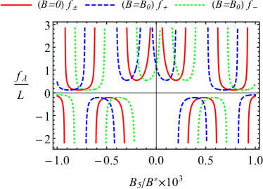
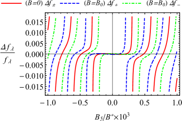
Figure 2: Left panel: The focal length $f_{\lambda}$ for the quasiparticles of given chirality $\lambda$ as a function of the pseudomagnetic field. Right panel: The relative difference between the focal lengths with and without the Berry curvature effects $\Delta f_{\lambda}/f_{\lambda}$ as a function of the pseudomagnetic field. While the red solid lines correspond to quasiparticles of both chiralities at $B=0$, the blue dashed and green dotted lines represent the right- and left-handed quasiparticles at $B=10^{-4}B^{*}$, respectively. We set $\varepsilon=100~{}\mbox{meV}$ and $L=10^{-2}~{}\mbox{cm}$.

In order to illuminate the effects of the Berry curvature, it is instructive to compare the focal length in Eq. (9) with its counterpart when such effects are neglected, i.e.,

$$f_{\lambda}^{(0)}=\frac{l_{\varepsilon}B^{*}}{B_{\lambda}\sin{\left(\frac{LB_{\lambda}}{l_{\varepsilon}B^{*}}\right)}}.$$ (10)

The corresponding relative difference $\Delta f_{\lambda}/f_{\lambda}\equiv(f_{\lambda}^{(0)}-f_{\lambda})/f_{\lambda}$ is plotted in the right panel of Fig. 2 for $B=0$ and $B=10^{-4}B^{*}$. As one can see, away from the divergencies, the effects of the Berry curvature quantified by $\Delta f_{\lambda}$ are much smaller than the focal lengths. This fact is not surprising because the effects of the Berry curvature in Weyl materials are subleading compared to that of the combination of magnetic and pseudomagnetic fields. However, the corresponding effects may become noticeable at sufficiently large magnetic and pseudomagnetic fields or near the divergencies, where the Berry curvature corrections may lead to a noticeable spatial separation of the beams of chiral quasiparticles even by the ordinary magnetic field alone.

Just like in Weyl materials, a combination of the magnetic and pseudomagnetic lenses can be used for splitting the beams of chiral quasiparticles in Dirac materials. Naively, by taking into account the topological triviality of a Dirac point, one may suggest that the pseudomagnetic fields are absent and the spatial separation of the quasiparticles of different chiralities in magnetic and pseudomagnetic fields is impossible. However, some Dirac semimetals, e.g., $\mathrm{A_{3}Bi}$ ($\mathrm{A}=\mathrm{Na}$, $\mathrm{K}$, $\mathrm{Rb}$) as well as certain phases of $\mathrm{Cd_{3}As_{2}}$, are, in fact, hidden $\mathbb{Z}_{2}$ Weyl semimetals Gorbar:2014sja . Their Dirac points come from two pairs of superimposed Weyl nodes separated in the momentum space. Since the strain-induced pseudomagnetic field $\mathbf{B}_{5}$ is determined by the separation vector Cortijo:2016yph ; Pikulin:2016 ; Liu-Pikulin:2016 , this field will be the same in magnitude but opposite in direction for the corresponding two pairs of Weyl nodes. Therefore, if the Berry curvature effects were neglected as given by Eq. (10), the focal length of the right-handed (left-handed) quasiparticles from the first pair of Weyl nodes would coincide exactly with the focal length of the left-handed (right-handed) quasiparticles of the second pair of Weyl nodes. As a result, a generic beam of quasiparticles would split in two nonchiral beams after passing through the lens. In other words, there would be only valley separation with no spatial separation of the chirality. However, the Berry curvature qualitatively changes the situation and, according to Eq. (9), all focal lengths become different now. This is schematically illustrated in Fig. 3, where the beams of quasiparticles in Dirac semimetals under consideration are split into four chiral beams after passing through the lens. In summary, while the combination of magnetic and pseudomagnetic fields alone allows only for a valley separation in the Dirac materials, the inclusion of the Berry curvature effects is important in order to achieve the complete splitting of the beams. This is in contrast to the case of Weyl materials with two Weyl nodes where the Berry curvature provides only second-order corrections to the splitting induced by the (pseudo-)magnetic fields at the linear order.

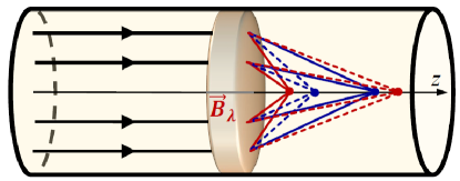
Figure 3: A schematic illustration of the spatial separation of chiral quasiparticles inside a Dirac semimetal crystal that is a $\mathbb{Z}_{2}$ Weyl semimetal. While the red lines correspond to the right-handed quasiparticles, the blue lines represent the left-handed ones. The solid and dashed lines correspond to the different pairs of Weyl nodes.

Lenses with a nonuniform background field. — It could be argued that the model situation with a constant (pseudo-)magnetic field $\mathbf{B}_{\lambda}$ considered above may not be very realistic. Indeed, for real solenoids and torsion-induced strains, there are always fringing fields at the ends. In order to get a better insight into the underlying physics, it is instructive to consider the case of a nonuniform (pseudo-)magnetic field with the following spatial profile:

$$\tilde{\mathbf{B}}_{\lambda}(z)=\theta(z)\theta\left(L-z\right)\frac{\mathbf{B}_{\lambda}}{1+\left(z-L/2\right)^{2}/\xi^{2}}.$$ (11)

Such a configuration mimics well the fringing fields at the ends of the (pseudo-)magnetic lens and, at the same time, allows one to obtain an analytical solution in the paraxial approximation. Because of the product of unit step functions $\theta(z)\theta\left(L-z\right)$ in Eq. (11), the effective field $\tilde{\mathbf{B}}_{\lambda}(z)$ is still effectively confined in the region $0<z<L$.

By limiting ourselves to the case of sufficiently weak (pseudo-)magnetic fields, we can neglect the effects of the Berry curvature in the eikonal approximation. This is supported by our findings presented in the right panel of Fig. 2, showing that the main contribution to the spatial separation of Weyl quasiparticles with different chirality comes from the leading linear order in the (pseudo-)magnetic field. Such an approximation also allows us to obtain explicit analytical results. When the quadratic corrections due to the Berry curvature are non-negligible, the corresponding analysis becomes much more involved but can be performed using numerical methods.

As is easy to check in the case of a weak inhomogeneity, i.e., $\xi\geq L$, the focal length $\tilde{f}_{\lambda}$ becomes almost indistinguishable from that in the uniform field shown in the left panel of Fig. 2. Of course, this is expected for a weakly varying (pseudo-)magnetic field. On the other hand, when the (pseudo-)magnetic field is sufficiently nonuniform, i.e., $\xi\lesssim L$, the dependence of $\tilde{f}_{\lambda}$ on the (pseudo-)magnetic field is different. (See Sec. III of the Supplemental Material for the details of solving the lens equation in a nonuniform field.) We note, however, that one can still use Eq. (10) for $\xi\lesssim L$, but with the following replacement of the lens size:

$$L\to L_{\rm eff}=\frac{1}{B_{\lambda}^{2}}\int_{-\infty}^{\infty}dz\left(\tilde{B}_{\lambda}(z)\right)^{2}=\frac{\pi\xi}{2},$$ (12)

where we used the explicit form of $\tilde{B}_{\lambda}(z)$ in Eq. (11) in order to perform the integration. Thus, the nonuniform (pseudo-)magnetic fields do not invalidate the principal possibility of pseudomagnetic lensing, albeit they may lead to some technical challenges in its experimental realization.

Conclusions. — In this study we investigated the conceptual possibility of pseudomagnetic lenses that can be used to focus the beams of chiral quasiparticles in Dirac and Weyl materials. We found that the maximum flexibility in controlling the beams of Weyl quasiparticles is achieved in the presence of both magnetic and pseudomagnetic fields. This allows one to achieve different magnitudes of the effective magnetic fields exerted on the left- and right-handed quasiparticles, which provides enough control to manipulate the focal lengths $f_{\lambda}$ independently for each chirality and valley. Moreover, in view of the nontrivial topology of Weyl fermions, the corresponding eikonal equation is affected by the Berry curvature leading to a splitting of the beams of chiral quasiparticles even by the ordinary magnetic field alone, albeit with a much smaller amplitude. Its effects are, however, crucial for the chirality separation in the Dirac semimetals, which comes on top of the valley separation induced by (pseudo-)magnetic fields. A similar generic separation is also expected in multipair Weyl materials.

It is intriguing to suggest that the pseudomagnetic lenses could allow for new and powerful ways of controlling and manipulating the chiral beams of quasiparticles inside Dirac and Weyl materials. For example, they may open an experimental possibility to control the spatial distributions of the electric current densities due to Weyl quasiparticles depending both on their valley and chirality that may be detected via local probes. By focusing the beams of the left- and right-handed quasiparticles in different spatial regions, one could achieve a “chiral distillation” and/or steady states of matter with a nonzero chiral asymmetry. We hope that findings of this study could lead to new applications that utilize the beam splitters of charged particles of given valley and chirality.

Supplemental Material: Pseudomagnetic lens as a valley and chirality splitter in Dirac and Weyl materials

I Key details of the eikonal approximation

In this section, using the standard eikonal approximation for charged particles [S1], we derive the equation for the abbreviated action $S_{0}\equiv S_{0}(\mathbf{r})$ of Weyl quasiparticles in the effective magnetic fields. We begin by making the following replacement in the dispersion relation (1) in the main text:

$$\mathbf{p}\to\bm{\nabla}S_{0}-\frac{e}{c}\mathbf{A}_{\lambda},$$ (S1)

where $\mathbf{A}_{\lambda}=\left(-yB_{\lambda}/2,xB_{\lambda}/2,0\right)$ is an effective vector potential that describes the background field $\mathbf{B}_{\lambda}$ in the $+z$ direction. Then, we obtain the following eikonal equation for the abbreviated action $S_{0}$ of Weyl quasiparticles with energy $\varepsilon$:

$$\varepsilon = v_{F}\sqrt{(\bm{\nabla}S_{0})^{2}+\frac{e^{2}}{4c^{2}}r_{\perp}^{2}B_{\lambda}^{2}}-\frac{\lambda e\hbar v_{F}B_{\lambda}}{2c}\frac{\nabla_{z}S_{0}}{(\bm{\nabla}S_{0})^{2}+\frac{e^{2}}{4c^{2}}r_{\perp}^{2}B_{\lambda}^{2}}$$ (S2)

$$+ \frac{e^{2}\hbar^{2}v_{F}B_{\lambda}^{2}}{8c^{2}}\frac{1}{\left[(\bm{\nabla}S_{0})^{2}+\frac{e^{2}}{4c^{2}}r_{\perp}^{2}B_{\lambda}^{2}\right]^{3/2}}-\frac{e^{2}\hbar^{2}v_{F}B_{\lambda}^{2}}{16c^{2}}\frac{(\nabla_{z}S_{0})^{2}}{\left[(\bm{\nabla}S_{0})^{2}+\frac{e^{2}}{4c^{2}}r_{\perp}^{2}B_{\lambda}^{2}\right]^{5/2}},$$

where, in view of the symmetry in the problem, we assumed that $S_{0}(\mathbf{r})$ depends on $z$ and $r_{\perp}=\sqrt{x^{2}+y^{2}}$, and used

$$\left(\bm{\nabla}S_{0}-\frac{e}{c}\mathbf{A}_{\lambda}\right)^{2}=(\bm{\nabla}S_{0})^{2}+\frac{e^{2}}{4c^{2}}r_{\perp}^{2}B_{\lambda}^{2}.$$ (S3)

In order to obtain an analytical solution to Eq. (S2), we will use the paraxial approximation. In other words, we will assume that $r_{\perp}$ is small and expand the solution in powers of $r_{\perp}$. Clearly, this approximation is adequate only when the beam of chiral quasiparticles remains close to the optical axis of the (pseudo-)magnetic lens. In practice, of course, this condition may break down and, then, one would have to reanalyze the problem by using numerical methods. In such a regime, various optical aberrations will appear and further complicate the situation. While all these issues may be of real importance for making pseudomagnetic lenses in practice, they are beyond the scope of the conceptual study presented here.

In the case $\mathbf{B}_{\lambda}=0$, the action should describe a free quasiparticle moving with momentum $\varepsilon/v_{F}$, i.e.,

$$S_{0}^{\rm(free)}=\frac{\varepsilon}{v_{F}}\sqrt{z^{2}+r_{\perp}^{2}}\approx\frac{\varepsilon}{v_{F}}\left(z+\frac{r_{\perp}^{2}}{2z}+O(r_{\perp}^{4})\right).$$ (S4)

In the case of a nonzero $\mathbf{B}_{\lambda}$, we seek $S_{0}$ in a similar form, which is given by Eq. (2) in the main text. Indeed, by matching the actions at the boundaries of the (pseudo-)magnetic lens, one can easily show that the eikonal of a quasiparticle moving in (pseudo-)magnetic fields should also contain only even powers of $r_{\perp}$.

By keeping the terms up to quadratic order in $r_{\perp}^{2}$ and $B_{\lambda}$, as well as making use of the following relations:

$$\nabla_{z}S_{0} = \frac{\varepsilon}{v_{F}}\left(C+\frac{r_{\perp}^{2}}{2}A^{\prime}(z)\right),$$ (S5)

$$(\bm{\nabla}S_{0})^{2} = (\nabla_{z}S_{0})^{2}+\left(\frac{\varepsilon r_{\perp}}{v_{F}}\right)^{2}(A(z))^{2}=\left(\frac{\varepsilon}{v_{F}}\right)^{2}C^{2}+\left(\frac{\varepsilon r_{\perp}}{v_{F}}\right)^{2}\left[CA^{\prime}(z)+(A(z))^{2}\right],$$ (S6)

we rewrite Eq. (S2) as

$$C^{4}-C^{6}+\left(2-3C^{2}\right)r_{\perp}^{2}C^{2}\left[CA^{\prime}(z)+(A(z))^{2}\right]+\frac{2\lambda B_{\lambda}}{B^{*}}\left\{C^{3}+r_{\perp}^{2}C\left[\frac{3}{2}CA^{\prime}(z)+(A(z))^{2}\right]\right\}$$

$$+\frac{1}{2}\left(\frac{B_{\lambda}}{B^{*}}\right)^{2}\left\{C^{2}+r_{\perp}^{2}\left[CA^{\prime}(z)-2(A(z))^{2}\right]\right\}-\frac{r_{\perp}^{2}eB_{\lambda}^{2}}{2c\hbar B^{*}}C^{4}=0.$$ (S7)

At the zeroth order in $r_{\perp}^{2}$, Eq. (S7) reduces to the following equation:

$$C^{4}-C^{6}+\frac{2\lambda B_{\lambda}}{B^{*}}C^{3}+\frac{1}{2}\left(\frac{B_{\lambda}}{B^{*}}\right)^{2}C^{2} = 0.$$ (S8)

This equation has four nontrivial solutions, i.e.,

$$C^{(1)}_{\pm} \simeq \pm 1+\lambda\frac{B_{\lambda}}{B^{*}}\mp\frac{5}{4}\left(\frac{B_{\lambda}}{B^{*}}\right)^{2}+O\left(\frac{B_{\lambda}^{3}}{(B^{*})^{3}}\right),$$ (S9)

$$C^{(2)}_{\pm} \simeq -\left(\lambda\pm\frac{1}{\sqrt{2}}\right)\frac{B_{\lambda}}{B^{*}}+O\left(\frac{B_{\lambda}^{3}}{(B^{*})^{3}}\right),$$ (S10)

where we used an expansion in powers of the small parameter $B_{\lambda}/B^{*}$. By taking into account that $C$ should be equal to one in the limit of vanishing fields [cf. Eqs. (2) in the main text and (S4)] we conclude that the physical solution is given by $C=C^{(1)}_{+}$.

Further, by equating the terms quadratic in $r_{\perp}$ in Eq. (S7), we obtain the first-order differential equation (4) in the main text for the function $A(z)$.

II Lens equation for the uniform fields

In this section we present the key steps of the derivation of the lens equation in the simplest case of uniform magnetic and pseudomagnetic fields, $B_{\lambda}=const$. In the regions $z<0$ and $z>L$, the fields are absent. Therefore, $a_{1}=1$ and $a_{2}=0$ there and the solutions to Eq. (4) in the main text are given by

$$A(z)\Big{|}_{z<0} = \frac{1}{z-z_{1}},$$ (S11)

$$A(z)\Big{|}_{z>L} = \frac{1}{z-z_{2}},$$ (S12)

where $z_{1}$ and $z_{2}$ are the integration constants that will be fixed by the boundary conditions. On the other hand, by solving Eq. (4) in the main text in the region with nonzero background fields, i.e., $0<z<L$, we obtain the following solution:

$$A(z)\Big{|}_{0<z<L}=a_{2}\cot{\left(\frac{a_{2}}{a_{1}}z+\phi\right)},$$ (S13)

where $\phi$ is another integration constant that should be also determined by matching the solutions for $A(z)$ at $z=0$ and $z=L$, i.e.,

$$-\frac{1}{z_{1}} = a_{2}\cot{\left(\phi\right)},$$ (S14)

$$a_{2}\cot{\left(\frac{a_{2}}{a_{1}}L+\phi\right)} = \frac{1}{L-z_{2}}.$$ (S15)

Finally, after excluding $\phi$ from these equations, we obtain the lens equation

$$(z_{1}+g_{\lambda})(z_{2}-h_{\lambda})=-f^{2}_{\lambda}.$$ (S16)

with

$$g_{\lambda} = \frac{1}{a_{2}}\cot{\left(\frac{a_{2}L}{a_{1}}\right)}\simeq\frac{l_{\varepsilon}B^{*}}{B_{\lambda}\left(1-\lambda B_{\lambda}/B^{*}\right)}\cot{\left(\frac{LB_{\lambda}\left(1-\lambda B_{\lambda}/B^{*}\right)}{l_{\varepsilon}B^{*}}\right)},$$ (S17)

$$f_{\lambda} = \frac{1}{a_{2}\sin{\left(\frac{a_{2}L}{a_{1}}\right)}}\simeq\frac{l_{\varepsilon}B^{*}}{B_{\lambda}\left(1-\lambda B_{\lambda}/B^{*}\right)\sin{\left(\frac{LB_{\lambda}\left(1-\lambda B_{\lambda}/B^{*}\right)}{l_{\varepsilon}B^{*}}\right)}},$$ (S18)

and $h_{\lambda}=L+g_{\lambda}$.

III Lens equation for the nonuniform fields

In this section we present the derivation of the lens equation as well as focal length $\tilde{f}_{\lambda}$ for the nonuniform effective magnetic field

$$\tilde{\mathbf{B}}_{\lambda}(z)=\theta(z)\theta\left(L-z\right)\frac{\mathbf{B}_{\lambda}}{1+\left(z-L/2\right)^{2}/\xi^{2}},$$ (S19)

neglecting the effects of the Berry curvature. In this case, we have $\varepsilon=v_{F}p$ instead of Eq. (1) in the main text. Therefore, the analog of the differential equation (4) in the main text reads

$$A^{\prime}(z)+(A(z))^{2}+\frac{e(\tilde{B}_{\lambda}(z))^{2}}{2c\hbar B^{*}}=0.$$ (S20)

Taking into account the explicit form of the effective field $\tilde{B}_{\lambda}(z)$ profile (S19), we obtain the following analytical solution inside the solenoid:

$$A(z)\Big{|}_{0<z<L}=\frac{2c_{0}\xi F_{\lambda}+ic_{0}(L-2z)-\left(L-2z+2i\xi F_{\lambda}\right)\exp{\left(2iF_{\lambda}\,\mbox{arccot}\left(\frac{2\xi}{L-2z}\right)\right)}}{2\left(\xi^{2}+\frac{(L-2z)^{2}}{4}\right)\left[\exp{\left(2iF_{\lambda}\,\mbox{arccot}\left(\frac{2\xi}{L-2z}\right)\right)}-ic_{0}\right]},$$ (S21)

where $c_{0}$ is an integration constant and

$$F_{\lambda}\equiv\sqrt{1+\left(\frac{\xi B_{\lambda}}{l_{\varepsilon}B^{*}}\right)^{2}}.$$ (S22)

By matching the solutions outside the solenoid (S12) with that in Eq. (S21) at $z=0$ and $z=L$, we obtain the following lens equation:

$$(z_{1}+\tilde{g}_{\lambda})(z_{2}-\tilde{h}_{\lambda})=-\tilde{f}_{\lambda}^{2},$$ (S23)

where $\tilde{h}_{\lambda}=L+\tilde{g}_{\lambda}$,

$$\tilde{g}_{\lambda}=(L^{2}+4\xi^{2})\frac{2\xi F_{\lambda}\cos{\left[2F_{\lambda}\,\mbox{arccot}\left(\frac{2\xi}{L}\right)\right]}+L\sin{\left[2F_{\lambda}\,\mbox{arccot}\left(\frac{2\xi}{L}\right)\right]}}{2\left(4\xi^{2}F_{\lambda}^{2}-L^{2}\right)\sin{\left[2F_{\lambda}\,\mbox{arccot}\left(\frac{2\xi}{L}\right)\right]-8L\xi F_{\lambda}\cos{\left[2F_{\lambda}\,\mbox{arccot}\left(\frac{2\xi}{L}\right)\right]}}},$$ (S24)

and

$$\tilde{f}_{\lambda}=\frac{\xi\left(L^{2}+4\xi^{2}\right)F_{\lambda}}{\left(4\xi^{2}F_{\lambda}^{2}-L^{2}\right)\sin{\left[2F_{\lambda}\,\mbox{arccot}\left(\frac{2\xi}{L}\right)\right]}-4L\xi F_{\lambda}\cos{\left[2F_{\lambda}\,\mbox{arccot}\left(\frac{2\xi}{L}\right)\right]}}.$$ (S25)

Further, it is easy to check that $\lim_{\xi\to\infty}\tilde{f}_{\lambda}=f_{\lambda}^{(0)}$, where $f_{\lambda}^{(0)}$ is the solution in the case of the homogeneous field given by Eq. (10) in the main text. The dependence of the focal length $\tilde{f}_{\lambda}$ on the pseudomagnetic field strength $B_{5}$ is presented in Fig. S1 for $\xi=0.3\,L$ (left panel) and $\xi=L$ (right panel). The results for a moderately large $\xi$ depicted in the right panel are almost indistinguishable from the case of a uniform field, as it should be for a weakly varying (pseudo-)magnetic field. On the other hand, when the (pseudo-)magnetic field is sufficiently nonuniform, i.e., $\xi\lesssim L$, the dependence of $\tilde{f}_{\lambda}$ on the (pseudo-)magnetic field is different. Comparing the left and right panels in Fig. S1, we see that the period of the focal length oscillations increases with decreasing $\xi$.

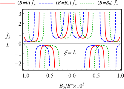
Figure S1: The focal length $\tilde{f}_{\lambda}$ for the nonuniform effective field (S19). While the red solid lines correspond to the quasiparticles of both chiralities at $B=0$, the blue dashed and green dotted lines represent the focal lengths for $\lambda=+$ and $\lambda=-$ at $B_{0}=10^{-4}B^{*}$, respectively. The left panel represents the results at $\xi=0.3\,L$ and the right one corresponds to $\xi=L$. We set $\varepsilon=100~{}\mbox{meV}$ and $L=10^{-2}~{}\mbox{cm}$.

 

• ] L. D. Landau and E. M. Lifshitz, The Classical theory of fields. Vol. 2 (Butterworth-Heinemann, Oxford, 1987).