Faster Greedy MAP Inference for Determinantal Point Processes

Abstract

Determinantal point processes (DPPs) are popular probabilistic models that arise in many machine learning tasks, where distributions of diverse sets are characterized by matrix determinants. In this paper, we develop fast algorithms to find the most likely configuration (MAP) of large-scale DPPs, which is NP-hard in general. Due to the submodular nature of the MAP objective, greedy algorithms have been used with empirical success. Greedy implementations require computation of log-determinants, matrix inverses or solving linear systems at each iteration. We present faster implementations of the greedy algorithms by utilizing the complementary benefits of two log-determinant approximation schemes: (a) first-order expansions to the matrix log-determinant function and (b) high-order expansions to the scalar log function with stochastic trace estimators. In our experiments, our algorithms are significantly faster than their competitors for large-scale instances, while sacrificing marginal accuracy.

1 Introduction

Determinantal point processes (DPPs) are elegant probabilistic models, first introduced by [25], who called them ‘fermion processes’. Since then, DPPs have been extensively studied in the fields of quantum physics and random matrices [14], giving rise to a beautiful theory [5]. The characteristic of DPPs is repulsive behavior, which makes them useful for modeling diversity.

Recently, they have been applied in many machine learning tasks such as summarization [9], human pose detection [20], clustering [16] and tweet time-line generation [36]. In particular, their computational advantage compared to other probabilistic models is that many important inference tasks are computationally tractable. For example, conditioning, sampling [16] and marginalization of DPPs admit polynomial-time/efficient algorithms, while those on popular graphical models [15] do not, i.e., they are NP-hard. One exception is the MAP inference (finding the most likely configuration), which is our main interest; the MAP computation is known to be NP-hard even for DPPs [20].

The distribution of diverse sets under DPPs is characterized by determinants of submatrices formed by their features, and the corresponding MAP inference reduces to finding a submatrix that maximizes its determinant. It is well known that the matrix log-determinant is a submodular function; that is, the MAP inference of DPPs is a special instance of submodular maximization [20]. Greedy algorithms have been shown to have the best worst-case approximation guarantees for many instances of submodular maximization; for example, $(1-1/e)$-approximation for monotone functions. Furthermore, it has been often empirically observed that greedy algorithms provide near optimal solutions [18]. Hence, greedy algorithms have been also applied for the DPP task [20, 36, 37]. Known implementations of greedy selection on DPP require computation of log-determinants, matrix inversions [20] or solving linear systems [23]. Consequently, they run in $O(d^{4})$ time where $d$ is the total number of items (see Section 2.3). In this paper, we propose faster greedy implementations that run in $O(d^{3})$ time.

Contribution. Our high-level idea is to amortize greedy operations by utilizing log-determinant approximation schemes. A greedy selection requires computation of marginal gains of log-determinants; we consider their first-order (linear) approximations. We observe that the computation of multiple marginal gains can be amortized into a single run of a linear solver, in addition to multiple vector inner products. We choose the popular conjugate gradient descent ($\mathtt{CG}$) [33] as a linear solver. In addition, for improving the quality of first-order approximations, we partition remaining items into $p\geq 1$ sets (via some clustering algorithm), and apply the first-order approximations in each partition. The resulting approximate computation of multiple marginal gains at each greedy selection requires $2p$ runs of $\mathtt{CG}$ under the Schur complement, and the overall running time of the proposed greedy algorithm becomes $O(d^{3})$ under the choice of $p=O(1)$ (see Section 3).

Next, for larger-scale DPPs, we develop an even faster greedy algorithm using a batch strategy. In addition to using the first-order approximations of log-determinants under a partitioning scheme, we add $k>1$ elements instead of a single element to the current set, where we sample some candidates among all possible $k$ elements to relax the expensive cost of computing all marginal gains. Intuitively, the random batch selection makes the algorithm $k$ times faster, while potentially hurting the approximation quality. Now, we suggest running the recent fast log-determinant approximation scheme ($\mathtt{LDAS}$) [11] $p$ times, instead of running $\mathtt{CG}$ $pk$ times under the Schur complement, where $\mathtt{LDAS}$ utilizes high-order, i.e., polynomial, approximations to the scalar log function with stochastic trace estimators. Since the complexities of running $\mathtt{LDAS}$ and $\mathtt{CG}$ are comparable, running the former $p$ times is faster than running the latter $pk$ times if $k>1$.

Finally, we discovered a novel scheme for boosting the approximation quality by sharing random vectors among many runs of $\mathtt{LDAS}$, and also establish theoretical justification why this helps. Our experiments on both synthetic and real-world dataset show that the proposed algorithms are significantly faster than competitors for large-scale instances, while losing marginal approximation ratio.

Related work. To the best of our knowledge, this is the first work that aims for developing faster greedy algorithms specialized for the MAP inference of DPP, while there has been several efforts on those for general submodular maximization. An accelerated greedy algorithm, called lazy evaluation, was first proposed by [27] which maintains the upper bounds on the marginal gains instead of recomputing exact values. In each iteration, only elements with the maximal bound compute the exact gain, which still bounds on the exact value due to submodularity. For the DPP case, we also observe that the lazy algorithm is significantly faster than the standard greedy one, while the outputs of both are equal. Hence, we compare our algorithms with the lazy one (see Section 6).

Another natural approach is on stochastic greedy selections computing marginal gains of randomly selected elements. Its worst-case approximation guarantee was also studied [28], under the standard, non-batch, greedy algorithm. The idea of stochastic selections can be also applied to our algorithms, where we indeed apply it for designing our faster batch greedy algorithm as mentioned earlier. Recently, [4] proposed a ‘one-pass’ greedy algorithm where each greedy selection requires computing only a single marginal gain, i.e., the number of marginal gains necessary to compute can be significantly reduced. However, this algorithm is attractive only for the case when evaluating a marginal gain does not increase with respect to the size of the current set, which does not hold for the DPP case. As reported in Section 6, it performs significantly worse than ours in both their approximation qualities and running times.

There have been also several efforts to design parallel/distributed implementations of greedy algorithms: [31] use parallel strategies for the above one-pass greedy algorithm and [21] adapt a MapReduce paradigm for implementing greedy algorithms in distributed settings. One can also parallelize our algorithms easily since they require independent runs of matrix-vector (or vector inner) products, but we do not explore this aspect in this paper. Finally, we remark that a non-greedy algorithm was studied in [8] for better MAP qualities of DPP, but it is much slower than ours as reported in Section 6.

Organization. We introduce the necessary background in Section 2, and present the proposed algorithms in Section 3 and Section 4. Proofs and Experimental results are presented in Section 5 and Section 6, respectively.

2 Preliminaries

We start by defining a necessary notation. Our algorithms for determinantal point processes (DPPs) select elements from the ground set of $d$ items $\mathcal{Y}=[d]:=\{1,2,\dots,d\}$ and denote the set of all subsets of $\mathcal{Y}$ by $2^{\mathcal{Y}}$. For any positive semidefinite matrix $L\in\mathbb{R}^{d\times d}$, we denote $\lambda_{\min}$ and $\lambda_{\max}$ to be the smallest and the largest eigenvalues of $L$. Given subset $X,Y\subseteq\mathcal{Y}$, we use $L_{X,Y}$ to denote the submatrix of $L$ obtained by entries in rows and columns indexed by $X$ and $Y$, respectively. For notational simplicity, we let $L_{X,X}=L_{X}$ and $L_{X,\{i\}}=L_{X,i}$ for $i\in\mathcal{Y}$. In addition, $\overline{L}_{X}$ is defined as the average of $L_{X\cup\{i\}}$ for $i\in\mathcal{Y}\setminus X$. Finally, $\left\langle\cdot,\cdot\right\rangle$ means the matrix/vector inner product or element-wise product sum.

In Section 2.1, we introduce the maximum a posteriori (MAP) inference of DPP, then the standard greedy optimization scheme and its naïve implementations are described in Section 2.2 and Section 2.3, respectively.

2.1 Determinantal Point Processes

DPPs are probabilistic models for subset selection of a finite ground set $\mathcal{Y}=[d]$ that captures both quality and diversity. Formally, it defines the following distribution on $2^{\mathcal{Y}}$: for random variable $\mathbf{X}\subseteq\mathcal{Y}$ drawn from given DPP, we have

$$\Pr\left[\mathbf{X}=X\right]\propto\det\left(L_{X}\right),$$

where $L\in\mathbb{R}^{d\times d}$ is a positive definite matrix called an $L$-ensemble kernel. Under the distribution, several probabilistic inference tasks are required for real-world applications, including MAP [9, 8, 36], sampling [17, 16, 22], marginalization and conditioning [9]. In particular, we are interested in the MAP inference, i.e., finding the most diverse subset $Y$ of $\mathcal{Y}$ that achieves the highest probability, i.e., $\arg\max_{Y\subseteq\mathcal{Y}}\det(L_{Y})$, possibly under some constraints on $Y$. Unlike other inference tasks on DPP, it is known that MAP is a NP-hard problem [20].

2.2 Greedy Submodular Maximization

A set function $f:2^{\mathcal{Y}}\rightarrow\mathbb{R}$ is submodular if its marginal gains are decreasing, i.e.,

$$f(X\cup\{i\})-f(X)\geq f(Y\cup\{i\})-f(Y),$$

for every $X\subseteq Y\subset\mathcal{Y}$ and every $i\in\mathcal{Y}\setminus Y$. We say $f$ is monotone if $f(X)\leq f(Y)$ for every $X\subseteq Y$. It is well known that DPP has the submodular structure, i.e., $f=\log\det$ is submodular.

The submodular maximization task is to find a subset maximizing a submodular function $f$, which corresponds to the MAP inference task in the DPP case. Hence, it is NP-hard and a popular approximate scheme is the following greedy procedure [29]: initially, $X\leftarrow\emptyset$ and iteratively update $X\leftarrow X\cup\{i_{\max}\}$ for

$$i_{\max}=\operatornamewithlimits{argmax}_{i\in\mathcal{Y}\setminus X}f({X\cup\{i\}})-f(X),$$ (1)

as long as $f({X\cup\{i_{\max}\}})>f({X})$. For the monotone case, it guarantees $(1-1/e)$-approximation [29]. Under some modifications of the standard greedy procedure, $2/5$-approximation can be guaranteed even for non-monotone functions [7]. Irrespectively of such theoretical guarantees, it has been empirically observed that greedy selection (1) provides near optimal solutions in practice [18, 34, 36, 37].

2.3 Naïve Implementations of Greedy Algorithm

Log-determinant or related computations, which are at the heart of greedy algorithms for MAP inference of DPPs, are critical to compute the marginal gain $\log\det L_{X\cup\{i\}}-\log\det L_{X}$. Since the exact computations of log-determinants might be slow, i.e., requires $O(d^{3})$ time for $d$-dimensional matrices, we introduce recent efficient log-determinant approximation schemes ($\mathtt{LDAS}$). The log-determinant of a symmetric positive definite matrix $A$ can be approximated by combining (a) Chebyshev polynomial expansion of scalar $\log$ function and (b) matrix trace estimators via Monte Carlo methods:

$$\log\det A={\tt tr}\left(\log A\right)\stackrel{{\scriptstyle(a)}}{{\approx}}{\tt tr}\left(p_{n}(A)\right)\stackrel{{\scriptstyle(b)}}{{\approx}}\frac{1}{m}\sum_{t=1}^{m}\mathbf{v}^{(t)\top}p_{n}(A)\mathbf{v}^{(t)}.$$

Here, $p_{n}(x)$ is a polynomial expansion of degree $n$ approximating $\log x$ and $\mathbf{v}^{(1)},\dots,\mathbf{v}^{(m)}$ are random vectors used for estimating the trace of $p_{n}(A)$. Several polynomial expansions, including Taylor [3], Chebyshev [11] and Legendre [32] have been studied. For trace estimation, several random vectors have been also studied [1], e.g., the Hutchinson method [13] chooses elements of $\mathbf{v}$ as i.i.d. random numbers in $\{-1,+1\}$ so that $\mathbf{E}\left[\mathbf{v}^{\top}A\mathbf{v}\right]={\tt tr}\left(A\right)$. In this paper, we use $\mathtt{LDAS}$ using the Chebyshev polynomial and Hutchinson method [11], but one can use other alternatives as well.

Log-determinant Approximation Scheme ($\mathtt{LDAS}$) [11]

  Input: symmetric matrix $A\in\mathbb{R}^{d\times d}$ with eigenvalues in $[\delta,1-\delta]$, sampling number $m$ and polynomial degree $n$

  Initialize: $\Gamma\leftarrow 0$

  $c_{j}\leftarrow$ $j$-th coefficient of Chebyshev expansion of $\log x$ on $[\delta,1-\delta]$ for $0\leq j\leq n$.

  for $i=1$ to $m$ do

     Draw a random vector $\mathbf{v}^{(i)}\in\{-1,+1\}^{d}$ whose entries are uniformly distributed.

     $\mathbf{w}_{0}^{(i)}\leftarrow\mathbf{v}^{(i)}$ and $\mathbf{w}_{1}^{(i)}\leftarrow\frac{2}{1-2\delta}A\mathbf{v}^{(i)}-\frac{1}{1-2\delta}\mathbf{v}^{(i)}$

     $\mathbf{u}\leftarrow c_{0}\mathbf{w}_{0}^{(i)}+c_{1}\mathbf{w}_{1}^{(i)}$

     for $j=2$ to $n$ do

        $\mathbf{w}_{2}^{(i)}\leftarrow\frac{4}{1-2\delta}A\mathbf{w}_{1}^{(i)}-\frac{2}{1-2\delta}\mathbf{w}_{1}^{(i)}-\mathbf{w}_{0}^{(i)}$

        $\mathbf{u}\leftarrow\mathbf{u}+c_{j}\ \mathbf{w}_{2}^{(i)}$

        $\mathbf{w}_{0}^{(i)}\leftarrow\mathbf{w}_{1}^{(i)}$ and $\mathbf{w}_{1}^{(i)}\leftarrow\mathbf{w}_{2}^{(i)}$

     end for

     $\Gamma\leftarrow\Gamma+\mathbf{v}^{(i)\top}\mathbf{u}/m$

  end for

  Output: $\Gamma$

Observe that $\mathtt{LDAS}$ only requires matrix-vector multiplications and its running time is $\Theta\left(d^{2}\right)$ for constants $m,n=O(1)$. One can directly use $\mathtt{LDAS}$ for computing (1) and the resulting greedy algorithm runs in $\Theta(d\cdot T_{\mathtt{GR}}^{3})$ time where the number of greedy updates on the current set $X$ is $T_{\mathtt{GR}}$. Since $T_{\mathtt{GR}}=O(d)$, the complexity is simply $O(d^{4})$. An alternative way to achieve the same complexity is to use the Schur complement [30]:

$$\log\det L_{X\cup\{i\}}-\log\det L_{X}=\log\left(L_{i,i}-L_{i,X}L_{X}^{-1}L_{X,i}\right).$$ (2)

This requires a linear solver to compute $L_{X}^{-1}L_{X,i}$; conjugate gradient descent ($\mathtt{CG}$) [10] is a popular choice in practice. Hence, if one applies $\mathtt{CG}$ to compute the max-marginal gain (1), the resulting greedy algorithm runs in $\Theta(d\cdot T_{\mathtt{GR}}^{3}\cdot T_{\mathtt{CG}})$ time, where $T_{\mathtt{CG}}$ denotes the number of iterations of each $\mathtt{CG}$ run. In the worst case, $\mathtt{CG}$ converges to the exact solution when $T_{\mathtt{CG}}$ grows with the matrix dimension, but for practical purposes, it typically provides a very accurate solution in few iterations, i.e., $T_{\mathtt{CG}}=O(1)$. Recently, Gauss quadrature via Lanczos iteration is used for efficient computing of $L_{i,X}L_{X}^{-1}L_{X,i}$ [23]. Although it guarantees rigorous upper/lower bounds, $\mathtt{CG}$ is faster and accurate enough for most practical purposes.

In summary, the greedy MAP inference of DPP can be implemented efficiently via $\mathtt{LDAS}$ or $\mathtt{CG}$. The faster implementations proposed in this paper smartly employ both of them as key components utilizing their complementary benefits.

3 Faster Greedy DPP Inference

In this section, we provide a faster greedy submodular maximization scheme for the MAP inference of DPP. We explain our key ideas in Section 3.1 and then, provide the formal algorithm description in Section 3.2.

3.1 Key Ideas

First-order approximation of log-determinant. The main computational bottleneck of a greedy algorithm is to evaluate the marginal gain (1) for every element not in the current set. To reduce the time complexity, we consider the following first-order, i.e., linear, approximation of log-determinant as:

$$\operatornamewithlimits{argmax}_{i\in\mathcal{Y}\setminus X}\log\det L_{X\cup\{i\}}-\log\det{L}_{X} =\operatornamewithlimits{argmax}_{i\in\mathcal{Y}\setminus X}\log\det L_{X\cup\{i\}}-\log\det\overline{L}_{X}$$

$$\approx\operatornamewithlimits{argmax}_{i\in\mathcal{Y}\setminus X}\left\langle{\overline{L}_{X}^{-1}},L_{X\cup\{i\}}-{\overline{L}_{X}}\right\rangle,$$ (3)

where we recall that $\overline{L}_{X}$ is the average of $L_{X\cup\{i\}}$. Observe that computing (3) requires the vector inner product of a single column (or row) of $\overline{L}_{X}^{-1}$ and $L_{X\cup\{i\}}-\overline{L}_{X}$ because $L_{X\cup\{i\}}$ and $\overline{L}_{X}$ share almost all entries except a single row and a column.

To obtain a single column of $\overline{L}_{X}^{-1}$, one can solve a linear system using the $\mathtt{CG}$ algorithm. More importantly, it suffices to run $\mathtt{CG}$ once for computing (3), while the naïve greedy implementation in Section 2.3 has to run $\mathtt{CG}$ $|\mathcal{Y}\setminus X|$ times. As we mentioned earlier, after obtaining the single column of $\overline{L}_{X}^{-1}$ using $\mathtt{CG}$, one has to perform $|\mathcal{Y}\setminus X|$ vector inner products in (3), but it is much cheaper than $|\mathcal{Y}\setminus X|$ $\mathtt{CG}$ runs requiring matrix-vector multiplications.

Partitioning. In order to further improve the quality of first-order approximation (3), we partition $\mathcal{Y}\setminus X$ into $p$ distinct subsets so that

$$\|L_{X\cup\{i\}}-\overline{L}_{X}\|_{F}~{}~{}\gg~{}~{}\|L_{X\cup\{i\}}-\overline{L}_{X}^{(j)}\|_{F},$$

where an element $i$ is in the partition $j\in\left[p\right]$, $\overline{L}_{X}^{(j)}$ is the average of $L_{X\cup\{i\}}$ for $i$ in the partition $j$, and $\left\lVert\cdot\right\rVert_{F}$ is the Frobenius norm. Since $L_{X\cup\{i\}}$ becomes closer to the average $\overline{L}_{X}^{(j)}$, one can expect that the first-order approximation quality in (3) is improved. But, we now need a more expensive procedure to approximate the marginal gain:

$$\log\det L_{X\cup\{i\}}-\log\det{L}_{X}$$

$$=\left(\log\det L_{X\cup\{i\}}-\log\det\overline{L}_{X}^{(j)}\right)+\left(\log\det\overline{L}_{X}^{(j)}-\log\det{L}_{X}\right)$$

$$\approx\underbrace{\left\langle{\left(\overline{L}_{X}^{(j)}\right)^{-1}},L_{X\cup\{i\}}-{\overline{L}_{X}^{(j)}}\right\rangle}_{(a)}+\underbrace{\left(\log\det\overline{L}_{X}^{(j)}-\log\det{L}_{X}\right)}_{(b)}.$$

The first term (a) can be computed efficiently as we explained earlier, but we have to run $\mathtt{CG}$ $p$ times for computing single columns of $\overline{L}_{X}^{(1)},\dots,\overline{L}_{X}^{(p)}$. The second term (b) can be also computed using $\mathtt{CG}$ similarly to (2) under the Schur complement. Hence, one has to run $\mathtt{CG}$ $2p$ times in total. If $p$ is large, the overall complexity becomes larger, but the approximation quality improves as well. We also note that one can try various clustering algorithms, e.g., $k$-means or Gaussian mixture. Instead, we use a simple random partitioning scheme because it is not only the fastest method but it also works well in our experiments.

3.2 Algorithm Description and Guarantee

The formal description of the proposed algorithm is described in Algorithm 1.

Algorithm 1 Faster Greedy DPP Inference

1:  Input: kernel matrix $L\in\mathbb{R}^{d\times d}$ and number of partitions $p$

2:  Initialize: $X\leftarrow\emptyset$

3:  while $\mathcal{Y}\setminus X\neq\emptyset$ do

4:     Partition $\mathcal{Y}\setminus X$ randomly into $p$ subsets.

5:     for $j=1$ to $p$ do

6:        $\overline{L}_{X}^{(j)}\leftarrow\text{average of }L_{X\cup\{i\}}$ for $i$ in the partition $j$

7:        $\mathbf{z}^{(j)}\leftarrow$ $\left(|X|+1\right)$-th column of $\left(\overline{L}_{X}^{(j)}\right)^{-1}$

8:        ${\Gamma}_{j}\leftarrow\log\det\overline{L}_{X}^{(j)}-\log\det L_{X}$

9:     end for

10:     for $i\in\mathcal{Y}\setminus X$ do

11:        ${\Delta}_{i}\leftarrow\left\langle L_{X\cup\{i\}}-{\overline{L}_{X}^{(j)}},\mathtt{Mat}\left(\mathbf{z}^{(j)}\right)\right\rangle+\Gamma_{j}$where element $i$ is included in partition $j$.

12:     end for

13:     $i_{\max}\leftarrow\operatornamewithlimits{argmax}_{i\in\mathcal{Y}\setminus X}{\Delta}_{i}$

14:     if $\log\det L_{X\cup\{i_{\max}\}}-\log\det L_{X}<0$ then

15:        return $X$

16:     end if

17:     $X\leftarrow X\cup\{i_{\max}\}$

18:  end while

As we explained in Section 3.1, the lines 7, 8 require to run $\mathtt{CG}$. Hence, the overall complexity becomes $\Theta(T_{\mathtt{GR}}^{3}\cdot T_{\mathtt{CG}}\cdot p+d\cdot T_{\mathtt{GR}}^{2})=\Theta(T_{\mathtt{GR}}^{3}+d\cdot T_{\mathtt{GR}}^{2})$, where we choose $p,T_{\mathtt{CG}}=O(1)$. Since $T_{\mathtt{GR}}=O(d)$, it is simply $O(d^{3})$ and better than the complexity $O(d^{4})$ of the naïve implementations described in Section 2.3. In particular, if kernel matrix $L$ is sparse, i.e., number of non-zeros of each column/row is $O(1)$, ours has the complexity $\Theta(T_{\mathtt{GR}}^{2}+d\cdot T_{\mathtt{GR}})$ while the naïve approaches are still worse having the complexity $\Theta(d\cdot T_{\mathtt{GR}}^{2})$.

We also provide the following approximation guarantee of Algorithm 1 for the monotone case, where its proof is given in Section 5.1.

Theorem 1.

Suppose the smallest eigenvalue of $L$ is greater than 1. Then, it holds that

$$\log\det L_{X}\geq\left(1-1/e\right)\max_{Z\subseteq\mathcal{Y},|Z|=|X|}\log\det L_{Z}-2|X|\varepsilon.$$

where

$$\varepsilon=\max_{X\subseteq\mathcal{Y},i\in\mathcal{Y}\setminus X\atop j\in\left[p\right]}\left|\log\frac{\det L_{X\cup\{i\}}}{\det\overline{L}_{X}^{(j)}}-\left\langle\left(\overline{L}_{X}^{(j)}\right)^{-1},L_{X\cup\{i\}}-\overline{L}_{X}^{(j)}\right\rangle\right|$$

and $X$ is the output of Algorithm 1.

The above theorem captures the relation between the first-order approximation error $\varepsilon>0$ in (3) and the worst-case approximation ratio of the algorithm.

4 Faster Batch-Greedy DPP Inference

In this section, we present an even faster greedy algorithm for the MAP inference task of DPP, in particular for large-scale tasks. On top of ideas described in Section 3.1, we use a batch strategy, i.e., add $k$ elements instead of a single element to the current set, where $\mathtt{LDAS}$ in Section 2.3 is now used as a key component. The batch strategy accelerates our algorithm. We first provide the formal description of the batch greedy algorithm in Section 4.1. In Section 4.2, we describe additional ideas on applying $\mathtt{LDAS}$ as a subroutine of the proposed batch algorithm.

4.1 Algorithm Description

Algorithm 2 Faster Batch-Greedy DPP Inference

1:  Input: kernel matrix $L\in\mathbb{R}^{d\times d}$, number of partitions $p$, batch size $k$ and the number of batch samples $s$

2:  Initialize: $X\leftarrow\emptyset$

3:  while $\mathcal{Y}\setminus X$ is not empty do

4:     $I_{i}\leftarrow$ Randomly draw a batch of size $k$ for $i\in\left[s\right]$.

5:     Partition $\left[s\right]$ randomly into $p$ subsets.

6:     for $j=1$ to $p$ do

7:        $\overline{L}_{X}^{(j)}\leftarrow\text{average of }L_{X\cup I_{i}}$ for $i$ in the partition $j$

8:        $Z^{(j)}\leftarrow(|X|+1)$ to $(|X|+k)$-th columns of $\left(\overline{L}_{X}^{(j)}\right)^{-1}$

9:        ${\Gamma}_{j}\leftarrow\log\det\overline{L}_{X}^{(j)}$ using $\mathtt{LDAS}$.

10:     end for

11:     for $i=1$ to $s$ do

12:        ${\Delta}^{\text{Batch}}_{i}\leftarrow\left\langle L_{X\cup I_{i}}-{\overline{L}_{X}^{(j)}},\mathtt{Mat}\left(Z^{(j)}\right)\right\rangle+\Gamma_{j}$ where a batch index $i$ is included in $j$-th partition.

13:     end for

14:     $i_{\max}\leftarrow\operatornamewithlimits{argmax}_{i\in[s]}\Delta^{\text{Batch}}_{i}$

15:     if $\log\det L_{X\cup I_{i_{\max}}}-\log\det L_{X}<0$ then

16:        return $X$

17:     end if

18:     $X\leftarrow X\cup I_{i_{\max}}$

19:  end while

The formal description of the proposed algorithm is described in Algorithm 2. Similar to the line 7 in Algorithm 1, the line 8 of Algorithm 2 can be solved by the $\mathtt{CG}$ algorithms. However, the line 9 of Algorithm 2 uses the $\mathtt{LDAS}$ and we remind that it runs in $\Theta(d^{2})$ time. In addition, the line 12 requires the vector inner products $ks$ times. Thus, the total complexity becomes $\Theta\left(T_{\mathtt{GR}}^{3}\cdot\left(T_{\mathtt{CG}}+\frac{mn}{k}\right)\cdot p+s\cdot T_{\mathtt{GR}}^{2}+s\cdot T_{\mathtt{CG}}\right)=\Theta(T_{\mathtt{GR}}^{3})$ where $T_{\mathtt{GR}}$ is the number of greedy updates on the current set $X$ and we choose all parameters $p,T_{\mathtt{CG}},k,s,m,n=O(1)$. We note that Algorithm 2 is expected to perform faster than Algorithm 1 when both $T_{\mathtt{GR}}$ and $d$ are large. This is primarily because the size of the current set $X$ increases by $k>1$ for each greedy iteration. A larger choice of $k$ speeds up the algorithm up to $k$ times, but it might hurt its output quality. We explain more details of key components of the batch algorithm below.

Batch selection. The essence of Algorithm 2 is adding $k>1$ elements, called batch, simultaneously to the current set with an improved marginal gain. Formally, it starts from the empty set and recursively updates $X\leftarrow X\cup I_{\max}$ for

$$I_{\max}=\operatornamewithlimits{argmax}_{I\subseteq\mathcal{Y}\setminus X,|I|=k}\log\det L_{X\cup I}.$$ (4)

until no gain is attained. The non-batch greedy procedure (1) corresponds to $k=1$. Such batch greedy algorithms have been also studied for submodular maximization [29, 12] and recently, [24] studied their theoretical guarantees showing that they can be better than their non-batch counterparts under some conditions. The main drawback of the standard batch greedy algorithms is that finding the optimal batch of size $k$ requires computing too many marginal gains of $\binom{|\mathcal{Y}\setminus X|}{k}$ subsets. To address the issue, we sample $s\ll\binom{|\mathcal{Y}\setminus X|}{k}$ bunches of batch subsets randomly and compute approximate batch marginal gains using them. [28] first propose an uniformly random sampling to the standard non-batch greedy algorithm. The authors show that it guarantees $(1-1/e-O(e^{-s}))$ approximation ratio in expectation and report that it performs well in many applications. In our experiments, we choose $s=50$ batch samples.

High-order approximation of log-determinant. Recall that for Algorithm 1, we suggest using the $\mathtt{CG}$ algorithm under the Schur complement for computing

$$\log\det\overline{L}_{X}^{(j)}-\log\det{L}_{X}.$$ (5)

One can apply the same strategy for Algorithm 2, which requires running the $\mathtt{CG}$ algorithm $k$ times for (5). Instead, we suggest running $\mathtt{LDAS}$ (using polynomial/high-order approximations of the scalar log function) only once, i.e., the line 9, which is much faster if $k$ is large. We remind that the asymptotic complexities of $\mathtt{CG}$ and $\mathtt{LDAS}$ are comparable.

4.2 Sharing Randomness in Trace Estimators

To improve the approximation quality of Algorithm 2, we further suggest running $\mathtt{LDAS}$ using the same random vectors $\mathbf{v}^{(1)},\dots,\mathbf{v}^{(m)}$ across $j\in\left[p\right]$. This is because we are interested in relative values $\log\det\overline{L}_{X}^{(j)}$ for $j\in\left[p\right]$ instead of their absolute ones.

Figure 1: Log-determinant estimation qualities of $\mathtt{LDAS}$ for sharing and independent random vectors.

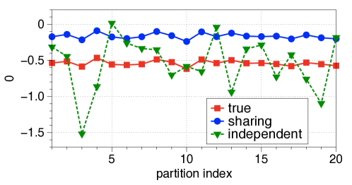
Our intuition is that different random vectors have different bias, which hurt the comparison task. Figure 1 demonstrates an experiment on the estimation of $\log\det\overline{L}_{X}^{(j)}$ when random vectors are shared and independent, respectively. This implies that sharing random vectors might be worse for estimating the absolute values of log-determinants, but better for comparing them.

We also formally justify the idea of sharing random vectors as stated in the follows theorem whose proof is given in Section 5.2.

Theorem 2.

Suppose $A,B$ are positive definite matrices whose eigenvalues are in $\left[\delta,1-\delta\right]$ for $\delta>0$. Let $\Gamma_{A},\Gamma_{B}$ be the estimations of $\log\det A$, $\log\det B$ by $\mathtt{LDAS}$ using the same random vectors $\mathbf{v}^{(1)},\dots,\mathbf{v}^{(m)}$ for both. Then, it holds that

$$\mathbf{Var}\left[\Gamma_{A}-\Gamma_{B}\right]\leq\frac{32M^{2}\rho^{2}\left(\rho+1\right)^{2}}{m\left(\rho-1\right)^{6}\left(1-2\delta\right)^{2}}\|A-B\|_{F}^{2}$$

where $M=5\log\left(2/\delta\right)$ and $\rho=1+\frac{2}{\sqrt{2/\delta-1}-1}$.

Without sharing random vectors, the variance should grow linearly with respect to $\left\lVert A\right\rVert_{F}^{2}+\left\lVert B\right\rVert_{F}^{2}$. In our case, matrices $A$ and $B$ correspond to some of $\overline{L}_{X}^{(j)}$, and $\|A-B\|_{F}^{2}$ is significantly smaller than $\left\lVert A\right\rVert_{F}^{2}+\left\lVert B\right\rVert_{F}^{2}$. We believe that our idea of sharing randomness might be of broader interest in many applications of $\mathtt{LDAS}$ or its variants, requiring multiple log-determinant computations.

5 Proof of Theorems

In this section, we provide the proof of our main theorems.

5.1 Proof of Theorem 1

For given $X\subseteq\mathcal{Y}$, we denote that the true marginal gain $\Lambda_{i}$ and the approximated gain $\Delta_{i}$ (used in Algorithm 1) as

$$\Lambda_{i} :=\log\det L_{X\cup\{i\}}-\log\det L_{X},$$

$$\Delta_{i} :=\left\langle{\left(\overline{L}_{X}^{(j)}\right)^{-1}},L_{X\cup\{i\}}-{\overline{L}_{X}^{(j)}}\right\rangle+\left(\log\det\overline{L}_{X}^{(j)}-\log\det{L}_{X}\right)$$

where an item $i\in\mathcal{Y}\setminus X$ is in the partition $j$. We also use $i_{\mathtt{OPT}}=\operatornamewithlimits{argmax}_{i}\Lambda_{i}$ and $i_{\max}=\operatornamewithlimits{argmax}_{i}\Delta_{i}$. Then, we have

$$\Lambda_{i_{\max}}{\geq}\ \Delta_{i_{\max}}-\varepsilon\ {\geq}\ \Delta_{i_{\mathtt{OPT}}}-\varepsilon\ {\geq}\ \Lambda_{i_{\mathtt{OPT}}}-2\varepsilon\$$

where the first and third inequalities are from the definition of $\varepsilon$, i.e., $\left|\Lambda_{i}-\Delta_{i}\right|\leq\varepsilon$, and the second inequality holds by the optimality of $i_{\max}$. In addition, when the smallest eigenvalue of $L$ is greater than 1, $\log\det L_{X}$ is monotone and non-negative [34]. To complete the proof, we introduce following approximation guarantee of the greedy algorithm with a ‘noise’ during the selection [35].

Theorem 3.

(Noisy greedy algorithm) Suppose a submodular function $f$ defined on ground set $\mathcal{Y}$ is monotone and non-negative. Let $X_{0}=\emptyset$ and $X_{k}=X_{k-1}\cup\{i_{\max}\}$ such that

$$f(X_{k-1}\cup\{i_{\max}\})-f(X_{k-1})\geq\max_{i\in\mathcal{Y}\setminus X_{k-1}}\left(f(X_{k-1}\cup\{i\})-f(X_{k-1})\right)-\varepsilon_{k}$$

for some $\varepsilon_{k}\geq 0$. Then,

$$f(X_{k})\geq\left(1-1/e\right)\max_{X\subseteq\mathcal{Y},|X|\leq k}f(X)-\sum_{i=1}^{k}\varepsilon_{i}$$

Theorem 1 is straightforward by substituting $2\varepsilon$ into $\varepsilon_{k}$. This completes the proof of Theorem 1.

5.2 Proof of Theorem 2

As we explained in Section 2.3, Chebyshev expansion of $\log x$ in $[\delta,1-\delta]$ with degree $n$ is defined as $p_{n}\left({x}\right)$. This can be written as

$$p_{n}\left({x}\right)=\sum_{k=0}^{n}c_{k}T_{k}\left(\frac{2}{1-2\delta}x-\frac{1}{1-2\delta}\right)$$ (6)

where the coefficient $c_{k}$ and the $k$-th Chebyshev polynomial $T_{k}(x)$ are defined as

$$c_{k}=\begin{dcases}\frac{1}{n+1}\sum_{j=0}^{n}f\left(\frac{1-2\delta}{2}x_{j}+\frac{1}{2}\right)\ T_{0}(x_{j})&\text{if $\ k=0$}\\ \frac{2}{n+1}\sum_{j=0}^{n}f\left(\frac{1-2\delta}{2}x_{j}+\frac{1}{2}\right)\ T_{k}(x_{j})&\text{otherwise}\end{dcases}$$ (7)

$$T_{k+1}(x)=2xT_{k}(x)-T_{k-1}(x)\qquad\text{for $\ k\geq 1$}$$ (8)

where $x_{j}=\cos\left(\frac{\pi(j+1/2)}{n+1}\right)$ for $j=0,1,\dots,n$ and $T_{0}(x)=1$, $T_{1}(x)=x$ [26]. For simplicity, we now use $H:=p_{n}\left({A}\right)-p_{n}\left({B}\right)$ and denote $\widetilde{A}=\frac{2}{1-2\delta}A-\frac{1}{1-2\delta}\mathbf{I}$ where $\mathbf{I}$ is identity matrix with same dimension of $A$ and same for $\widetilde{B}$.

We estimate the log-determinant difference while random vectors are shared, i.e.,

$$\log\det A-\log\det B\approx\frac{1}{m}\sum_{i=1}^{m}\mathbf{v}^{(i)\top}H\mathbf{v}^{(i)}.$$

To show that the variance of $\mathbf{v}^{(i)\top}H\mathbf{v}^{(i)}$ is small as $\left\lVert A-B\right\rVert_{F}$, we provide that

$$\mathbf{Var}\left[\frac{1}{m}\sum_{i=1}^{m}\mathbf{v}^{(i)\top}H\mathbf{v}^{(i)}\right] =\frac{1}{m}\mathbf{Var}\left[\mathbf{v}^{\top}H\mathbf{v}\right]$$

$$\leq\frac{2}{m}\left\lVert H\right\rVert_{F}^{2}=\frac{2}{m}\left\lVert p_{n}\left({A}\right)-p_{n}\left({B}\right)\right\rVert_{F}^{2}$$

$$\leq\frac{2}{m}\left(\sum_{k=0}^{n}\left|c_{k}\right|\left\lVert T_{k}\left(\widetilde{A}\right)-T_{k}\left(\widetilde{B}\right)\right\rVert_{F}\right)^{2}$$

where the first inequality holds from [1] and the second is from combining (6) with the triangle inequality. To complete the proof, we use the following two lemmas.

Lemma 4.

Let $T_{k}\left(\cdot\right)$ be Chebyshev polynomial with $k$-degree and symmetric matrices $B,E$ satisfied with $\left\lVert B\right\rVert_{2}\leq 1$, $\left\lVert B+E\right\rVert_{2}\leq 1$. Then, for $k\geq 0$,

$$\left\lVert T_{k}\left(B+E\right)-T_{k}\left(B\right)\right\rVert_{F}\leq k^{2}\left\lVert E\right\rVert_{F}.$$

Lemma 5.

Let $c_{k}$ be the $k$-th coefficient of Chebyshev expansion for $f\left(x\right)$. Suppose $f$ is analytic with $\left|f\left(z\right)\right|\leq M$ in the region bounded by the ellipse with foci $\pm 1$ and the length of major and minor semiaxis summing to $\rho>1$. Then,

$$\sum_{k=0}^{n}k^{2}\left|c_{k}\right|\leq\frac{2M\rho\left(\rho+1\right)}{\left(\rho-1\right)^{3}}.$$

In order to apply Lemma 5, we should consider $f(x)=\log\left(\frac{1-2\delta}{2}x+\frac{1}{2}\right)$. Then it can be easily obtained $M=5\log\left(2/\delta\right)$ and $\rho=1+\frac{2}{\sqrt{2/\delta-1}-1}$ as provided in [11].

Using Lemma 4 and 5, we can write

$$\mathbf{Var}\left[\frac{1}{m}\sum_{i=1}^{m}\mathbf{v}^{(i)\top}H\mathbf{v}^{(i)}\right] \leq\frac{2}{m}\left(\sum_{k=0}^{n}\left|c_{k}\right|\left\lVert T_{k}\left(\widetilde{A}\right)-T_{k}\left(\widetilde{B}\right)\right\rVert_{F}\right)^{2}$$

$$\leq\frac{2}{m}\left(\sum_{k=0}^{n}\left|c_{k}\right|k^{2}\left\lVert\widetilde{A}-\widetilde{B}\right\rVert_{F}\right)^{2}$$

$$\leq\frac{2}{m}\left(\frac{2M\rho\left(\rho+1\right)}{\left(\rho-1\right)^{3}}\right)^{2}\left(\frac{2}{1-2\delta}\left\lVert A-B\right\rVert_{F}\right)^{2}$$

$$=\frac{32M^{2}\rho^{2}\left(\rho+1\right)^{2}}{m\left(\rho-1\right)^{6}\left(1-2\delta\right)^{2}}\left\lVert A-B\right\rVert_{F}^{2}$$

where the second inequality holds from Lemma 4 and the thrid is from Lemma 5. This completes the proof of Theorem 2.

5.3 Proof of Lemma 4

Denote $R_{k}:=T_{k}\left(B+E\right)-T_{k}\left(B\right)$. From the recurrence of Chebyshev polynomial (8), $R_{k}$ has following

$$R_{k+1}=2\left(B+E\right)R_{k}-R_{k-1}+2E\ T_{k}\left(B\right)$$ (9)

for $k\geq 1$ where $R_{1}=E$, $R_{0}=\mathbf{0}$ where $\mathbf{0}$ is defined as zero matrix with the same dimension of $B$. Solving this, we obtain that

$$R_{k+1}=g_{k+1}\left(B+E\right)E+\sum_{i=0}^{k}h_{i}\left(B+E\right)E\ T_{k+1-i}\left(B\right)$$ (10)

for $k\geq 1$ where both $g_{k}\left(\cdot\right)$ and $h_{k}\left(\cdot\right)$ are polynomials with degree $k$ and they have following recurrences

$$g_{k+1}\left(x\right) =2xg_{k}\left(x\right)-g_{k-1}\left(x\right),g_{1}\left(x\right)=1,g_{0}\left(x\right)=0,$$

$$h_{k+1}\left(x\right) =2xh_{k}\left(x\right)-h_{k-1}\left(x\right),h_{1}\left(x\right)=2,h_{0}\left(x\right)=0.$$

In addition, we can easily verify that

$$2\max_{x\in\left[-1,1\right]}\left|g_{k}\left(x\right)\right|=\max_{x\in\left[-1,1\right]}\left|h_{k}\left(x\right)\right|=2k.$$

Putting all together, we conclude that

$$\left\lVert R_{k+1}\right\rVert_{F} \leq\left\lVert g_{k+1}\left(B+E\right)E\right\rVert_{F}+\left\lVert\sum_{i=0}^{k}h_{i}\left(B+E\right)E\ T_{k+1-i}\left(B\right)\right\rVert_{F}$$

$$\leq\left\lVert g_{k+1}\left(B+E\right)\right\rVert_{2}\left\lVert E\right\rVert_{F}+\sum_{i=0}^{k}\left\lVert h_{i}\left(B+E\right)\right\rVert_{2}\left\lVert E\right\rVert_{F}\left\lVert\ T_{k+1-i}\left(B\right)\right\rVert_{2}$$

$$\leq\left(\left\lVert g_{k+1}\left(B+E\right)\right\rVert_{2}+\sum_{i=0}^{k}\left\lVert h_{i}\left(B+E\right)\right\rVert_{2}\right)\left\lVert E\right\rVert_{F}$$

$$\leq\left(k+1+\sum_{i=0}^{k}2i\right)\left\lVert E\right\rVert_{F}$$

$$=\left(k+1\right)^{2}\left\lVert E\right\rVert_{F}$$

where the second inequality holds from $\left\lVert YX\right\rVert_{F}=\left\lVert XY\right\rVert_{F}\leq\left\lVert X\right\rVert_{2}\left\lVert Y\right\rVert_{F}$ for matrix $X,Y$ and the third inequality uses that $\left|T_{k}\left(x\right)\right|\leq 1$ for all $k\geq 0$. This completes the proof of Lemma 4.

5.4 Proof of Lemma 5

For general analytic function $f$, Chebyshev series of $f$ is defined as

$$f\left(x\right)=\frac{a_{0}}{2}+\sum_{k=1}^{\infty}a_{k}T_{k}\left(x\right),\quad a_{k}=\frac{2}{\pi}\int_{-1}^{1}\frac{f\left(x\right)T_{k}\left(x\right)}{\sqrt{1-x^{2}}}dx.$$

and from [26] it is known that

$$c_{k}-a_{k}=\sum_{j=1}^{\infty}\left(-1\right)^{j}\left(a_{2j(n+1)-k}+a_{2j(n+1)+k}\right)$$

and $\left|a_{k}\right|\leq\frac{2M}{\rho^{k}}$ for $0\leq k\leq n$. We remind that $c_{k}$ is defined in (7). Using this facts, we get

$$k^{2}\left|c_{k}\right| \leq k^{2}\left(\left|a_{k}\right|+\sum_{j=1}^{\infty}\left|a_{2j(n+1)-k}\right|+\left|a_{2j(n+1)+k}\right|\right)$$

$$\leq k^{2}\left|a_{k}\right|+\sum_{j=1}^{\infty}k^{2}\left|a_{2j(n+1)-k}\right|+k^{2}\left|a_{2j(n+1)+k}\right|$$

$$\leq k^{2}\left|a_{k}\right|+\sum_{j=1}^{\infty}\left(2j(n+1)-k\right)^{2}\left|a_{2j(n+1)-k}\right|+\left(2j(n+1)+k\right)^{2}\left|a_{2j(n+1)+k}\right|$$

Therefore, we have

$$\sum_{k=0}^{n}k^{2}\left|c_{k}\right|\leq\sum_{k=0}^{n}k^{2}\left|a_{k}\right|\leq\sum_{k=0}^{\infty}k^{2}\left|a_{k}\right|\leq\sum_{k=0}^{\infty}k^{2}\frac{2M}{\rho^{k}}=\frac{2M\rho\left(\rho+1\right)}{\left(\rho-1\right)^{3}}$$

This completes the proof of Lemma 5.

6 Experimental Results

In this section, we evaluate our proposed algorithms for the MAP inference on synthetic and real-world DPP instances.

Setups. The experiments are performed using a machine with a hexa-core Intel CPU (Core i7-5930K, 3.5 GHz) and 32 GB RAM. We compare our algorithms with following competitors: the lazy greedy algorithm (Lazy) [27], double greedy algorithm (Double) [4] and softmax extension (Softmax) [8]. In all our experiments, Lazy is significantly faster than the naïve greedy algorithms described in Section 2.3, while they produce the same outputs. Hence, we use Lazy as the baseline of evaluation.

Unless stated otherwise, we choose parameters of $p=5$, $k=10$, $s=50$, $m=20$ and $n=15$, regardless matrix dimension, for our algorithms. We also run $\mathtt{CG}$ until it achieves convergence error less than $10^{-10}$ and typically $T_{\mathtt{CG}}\leq 30$.

Additional tricks for boosting accuracy. For boosting approximation qualities of our algorithms, we use the simple trick in our experiments: recompute top $\ell$ marginal gains exactly (using $\mathtt{CG}$) where they are selected based on estimated marginal gains, i.e., $\Delta_{i}$ for Algorithm 1 and $\Delta^{\text{Batch}}_{i}$ for Algorithm 2. Then, our algorithms choose the best element among $\ell$ candidates, based on their exact marginal gains. Since we choose small $\ell=20$ in our experiments, this additional process increases the running times of our algorithms marginally, but makes them more accurate. In fact, the trick is inspired from [27] where the authors also recompute the exact marginal gains of few elements. In addition, for boosting further approximation qualities of Algorithm 2, we also run Algorithm 1 in parallel and choose the largest one among $\{\Delta_{i},\Delta^{\text{Batch}}_{i}\}$ given the current set. Hence, at most iterations, the batch with the maximal $\Delta^{\text{Batch}}_{i}$ is chosen and increases the current set size by $k$ (i.e., making speed-up) as like Algorithm 2, and the non-batch with the maximal $\Delta_{i}$ is chosen at very last iterations, which fine-tunes the solution quality. We still call the synthesized algorithm by Algorithm 2 in this section.

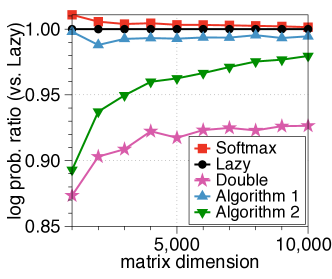
Performance metrics. For the performance measure on approximation qualities of algorithms, we use the following ratio of log-probabilities:

$${\log\det L_{X}}/{\log\det L_{X_{\textsc{Lazy}}}}.$$

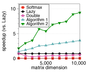
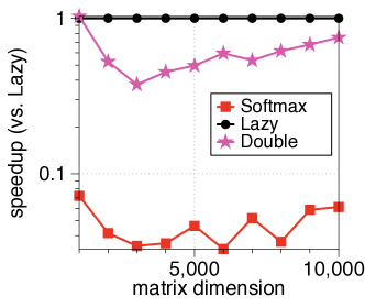
where $X$ and $X_{\textsc{Lazy}}$ are the outputs of an algorithm and Lazy, respectively. Namely, we compare outputs of algorithms with that of Lazy since the exact optimum is hard to compute. Similarly, we report the running time speedup of each algorithm over Lazy.

Figure 2: Plot of (a) log-probability ratio and (b), (c) and (d) implies speedup for Softmax, Double, Algorithm 1 and Algorithm 2 compared to Lazy, respectively. Algorithm 1 is about $3$ times faster the lazy greedy algorithm (Lazy) while loosing only $0.2\%$ accuracy at $d=10,000$. Algorithm 2 has $2\%$ loss on accuracy but $9$ times faster than Lazy at $d=10,000$. If dimension is $d=40,000$, it runs $19$ times faster.

6.1 Synthetic Dataset

In this section, we use synthetic DPP datasets generated as follows. As [19, 20] proposed, a kernel matrix $L$ for DPP can be re-parameterized as

$$L_{i,j}=q_{i}{\phi}_{i}^{\top}{\phi}_{j}q_{j},$$

where $q_{i}\in\mathbb{R}^{+}$ is considered as the quality of item $i$ and $\mathbf{\phi}_{i}\in\mathbb{R}^{d}$ is the normalized feature vector of item $i$ so that $\mathbf{\phi}_{i}^{\top}\mathbf{\phi}_{j}$ measures the similarity between $i$ and $j$. We use $q_{i}=\exp\left(\beta_{1}{x}_{i}+\beta_{2}\right)$ for the quality measurement ${x}_{i}\in\mathbb{R}$ and choose $\beta_{1}=0.01,\beta_{2}=0.2$. We choose each entry of $\phi_{i}$ and ${x}_{i}$ drawn from the normal distribution $\mathcal{N}(0,1)$ for all $i\in\left[d\right]$, and then normalize $\phi_{i}$ so that $\left\lVert\phi_{i}\right\rVert_{2}=1$.

Figure 3: Log-probability ratios compared to Lazy: (a) Algorithm 1 changing the number of clusters $p$ and (b) Algorithm 2 varying the batch size $k$. These experiments are done under $d=1,000$.

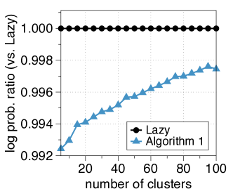
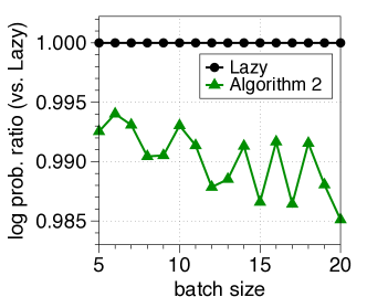
We first show how much the number of clusters $p$ and the batch size $k$ are sensitive for Algorithm 1 and Algorithm 2, respectively. Figure 3 shows the accuracy of Algorithm 1 with different numbers of clusters. It indeed confirms that a larger cluster improves its accuracy since it makes first-order approximations tighter. Figure 3 shows the performance trend of Algorithm 2 as the batch size $k$ increases, which shows that a larger batch might hurt its accuracy. Based on these experiments, we choose $p=5,k=10$ in order to target $0.01$ approximation ratio loss compared to Lazy.

We generate synthetic kernel matrices with varying dimension $d$ up to $40,000$, and the performances of tested algorithms are reported in Figure 2(a). One can observe that Lazy seems to be near-optimal, where only Softmax often provides marginally larger log-probabilities than Lazy under small dimensions. Interestingly, we found that Double has the strong theoretical guarantee for general submodular maximization [4], but its practical performance for DPP is worst among evaluating algorithms. Moverover, it is slightly slower than Lazy. In summary, one can conclude that our algorithms can be at orders of magnitude faster than Lazy, Double and Softmax, while loosing $0.01$-approximation ratio. For example, Algorithm 2 is $19$ times faster than Lazy for $d=40,000$, and the gap should increase for larger dimension $d$.

6.2 Real Dataset

We use real-world datasets of the following two tasks of matched and video summarizations.

Figure 4: Plot of log-probability ratio and speedup (log-scale) of Algorithm 2, compared to Lazy, for matched summarization under 2016 Republican presidential primaries.

Matched summarization. We evaluate our proposed algorithms for matched summarization that is first proposed by [8]. This task gives useful information for comparing the texts addressed at different times by the same speaker. Suppose we have two different documents and each one consists of several statements. The goal is to apply DPP for finding statement pairs that are similar to each other, while they summarize (i.e., diverse) well the two documents. We use transcripts of debates in 2016 US Republican party presidential primaries speeched by following $8$ participates: Bush, Carson, Christie, Kasich, Paul, Trump, Cruz and Rubio.

We follow similar pre-processing steps of [8]. First, every sentence is parsed and only nouns except the stopwords are extracted via NLTK [2]. Then, we remove the ‘rare’ words occurring less than $10\%$ of the whole debates, and then ignore each statement which contains more ‘rare’ words than ’frequent’ ones in it. This gives us a dataset containing $3,406$ distinct ‘frequent’ words and $1,157$ statements. For each statement pair $(i,j)$, feature vector $\phi_{(i,j)}=w_{i}+w_{j}\in\mathbb{R}^{3406}$ where $w_{i}$ is generated as a frequency of words in the statement $i$. Then, we normalize $\phi_{(i,j)}$. The match quality ${x}_{(i,j)}$ is measured as the cosine similarity between two statements $i$ and $j$, i.e., ${x}_{(i,j)}=w_{i}^{\top}w_{j}$, and we remove statement pairs $(i,j)$ such that its match quailty ${x}_{(i,j)}$ is smaller than $15\%$ of the maximum one. Finally, by choosing $q_{(i,j)}=\exp\left(0.01\cdot{x}_{(i,j)}\right)$, we obtain $\binom{8}{2}=28$ kernel matrices of dimension $d$ from $516$ to $4,000$.

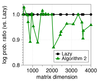
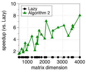
Figure 4 reports log-probability ratios and speedups of Algorithm 2 under the 28 kernels. We observe that Algorithm 2 looses $0.03$-approximation ratio on average, compared to Lazy, under the real-world kernels. Interestingly, Softmax runs much slower than even Lazy, while our algorithm runs faster than Lazy for large dimension, e.g., $8$ times faster for $d=4,000$ corresponding to transcripts of Bush and Rubio.

Figure 5: Plot of (a) F-scores for Algorithm 1 compared to Lazy and (b) speedup of both algorithms. (c) shows the summaries of YouTube video of index 99. Images in the first row are summaries produced by Lazy and the second row images illustrate those produced by Algorithm 1. The bottom 2 rows reflect ‘real’ user summaries.

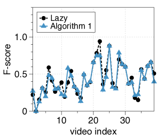
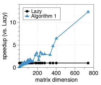
Video summarization. We evaluate our proposed algorithms video summarization. We use 39 videos from a Youtube dataset [6], and the trained DPP kernels from [9]. Under the kernels, we found that the numbers of selected elements from algorithms are typically small (less than 10), and hence we use Algorithm 1 instead of its batch version Algorithm 2. For performance evaluation, we use an F-score based on five sets of user summaries where it measures the quality across two summaries.

Figure 5 illustrates F-score for Lazy and Algorithm 1 and Figure 5 reports its speedup. Our algorithm achieves over 13 times speedup in this case, while it produces F-scores that are very similar to those of Lazy. For some video, it achieves even better F-score, as illustrated in 5.

7 Conclusion

We have presented fast algorithms for the MAP inference task of large-scale DPPs. Our main idea is to amortize common determinant computations via linear algebraic techniques and recent log-determinant approximation methods. Although we primarily focus on a special matrix optimization, we expect that several ideas developed in this paper would be useful for other related matrix computational problems, in particular, involving multiple determinant computations.

References

- Avron and Toledo, [2011] Avron, H. and Toledo, S. (2011). Randomized algorithms for estimating the trace of an implicit symmetric positive semi-definite matrix. Journal of the ACM (JACM), 58(2):8.
- Bird, [2006] Bird, S. (2006). Nltk: the natural language toolkit. In Proceedings of the COLING/ACL on Interactive presentation sessions, pages 69–72. Association for Computational Linguistics.
- Boutsidis et al., [2015] Boutsidis, C., Drineas, P., Kambadur, P., and Zouzias, A. (2015). A randomized algorithm for approximating the log determinant of a symmetric positive definite matrix. arXiv preprint arXiv:1503.00374.
- Buchbinder et al., [2015] Buchbinder, N., Feldman, M., Seffi, J., and Schwartz, R. (2015). A tight linear time (1/2)-approximation for unconstrained submodular maximization. SIAM Journal on Computing, 44(5):1384–1402.
- Daley and Vere-Jones, [2007] Daley, D. J. and Vere-Jones, D. (2007). An introduction to the theory of point processes: volume II: general theory and structure. Springer Science & Business Media.
- De Avila et al., [2011] De Avila, S. E. F., Lopes, A. P. B., da Luz, A., and de Albuquerque Araújo, A. (2011). Vsumm: A mechanism designed to produce static video summaries and a novel evaluation method. Pattern Recognition Letters, 32(1):56–68.
- Feige et al., [2011] Feige, U., Mirrokni, V. S., and Vondrak, J. (2011). Maximizing non-monotone submodular functions. SIAM Journal on Computing, 40(4):1133–1153.
- Gillenwater et al., [2012] Gillenwater, J., Kulesza, A., and Taskar, B. (2012). Near-optimal map inference for determinantal point processes. In Advances in Neural Information Processing Systems, pages 2735–2743.
- Gong et al., [2014] Gong, B., Chao, W.-L., Grauman, K., and Sha, F. (2014). Diverse sequential subset selection for supervised video summarization. In Advances in Neural Information Processing Systems, pages 2069–2077.
- Greenbaum, [1997] Greenbaum, A. (1997). Iterative methods for solving linear systems. SIAM.
- Han et al., [2015] Han, I., Malioutov, D., and Shin, J. (2015). Large-scale log-determinant computation through stochastic chebyshev expansions. In ICML, pages 908–917.
- Hausmann et al., [1980] Hausmann, D., Korte, B., and Jenkyns, T. (1980). Worst case analysis of greedy type algorithms for independence systems. In Combinatorial Optimization, pages 120–131. Springer.
- Hutchinson, [1990] Hutchinson, M. F. (1990). A stochastic estimator of the trace of the influence matrix for laplacian smoothing splines. Communications in Statistics-Simulation and Computation, 19(2):433–450.
- Johansson, [2006] Johansson, K. (2006). Course 1 random matrices and determinantal processes. Les Houches, 83:1–56.
- Jordan, [1998] Jordan, M. I. (1998). Learning in graphical models, volume 89. Springer Science & Business Media.
- Kang, [2013] Kang, B. (2013). Fast determinantal point process sampling with application to clustering. In Advances in Neural Information Processing Systems, pages 2319–2327.
- Kathuria and Deshpande, [2016] Kathuria, T. and Deshpande, A. (2016). On sampling and greedy map inference of constrained determinantal point processes. arXiv preprint arXiv:1607.01551.
- Krause et al., [2008] Krause, A., Singh, A., and Guestrin, C. (2008). Near-optimal sensor placements in gaussian processes: Theory, efficient algorithms and empirical studies. Journal of Machine Learning Research, 9(Feb):235–284.
- Kulesza and Taskar, [2011] Kulesza, A. and Taskar, B. (2011). Learning determinantal point processes. In In Proceedings of UAI. Citeseer.
- Kulesza et al., [2012] Kulesza, A., Taskar, B., et al. (2012). Determinantal point processes for machine learning. Foundations and Trends® in Machine Learning, 5(2–3):123–286.
- Kumar et al., [2015] Kumar, R., Moseley, B., Vassilvitskii, S., and Vattani, A. (2015). Fast greedy algorithms in mapreduce and streaming. ACM Transactions on Parallel Computing, 2(3):14.
- [22] Li, C., Jegelka, S., and Sra, S. (2016a). Efficient sampling for k-determinantal point processes. In Proceedings of the 19th International Conference on Artificial Intelligence and Statistics, pages 1328–1337.
- [23] Li, C., Sra, S., and Jegelka, S. (2016b). Gaussian quadrature for matrix inverse forms with applications. In Proceedings of The 33rd International Conference on Machine Learning, pages 1766–1775.
- Liu et al., [2016] Liu, Y., Zhang, Z., Chong, E. K., and Pezeshki, A. (2016). Performance bounds for the k-batch greedy strategy in optimization problems with curvature. In American Control Conference (ACC), 2016, pages 7177–7182. IEEE.
- Macchi, [1975] Macchi, O. (1975). The coincidence approach to stochastic point processes. Advances in Applied Probability, 7(01):83–122.
- Mason and Handscomb, [2002] Mason, J. C. and Handscomb, D. C. (2002). Chebyshev polynomials. CRC Press.
- Minoux, [1978] Minoux, M. (1978). Accelerated greedy algorithms for maximizing submodular set functions. In Optimization Techniques, pages 234–243. Springer.
- Mirzasoleiman et al., [2015] Mirzasoleiman, B., Badanidiyuru, A., Karbasi, A., Vondrák, J., and Krause, A. (2015). Lazier than lazy greedy. In Twenty-Ninth AAAI Conference on Artificial Intelligence.
- Nemhauser et al., [1978] Nemhauser, G. L., Wolsey, L. A., and Fisher, M. L. (1978). An analysis of approximations for maximizing submodular set functions—i. Mathematical Programming, 14(1):265–294.
- Ouellette, [1981] Ouellette, D. V. (1981). Schur complements and statistics. Linear Algebra and its Applications, 36:187–295.
- Pan et al., [2014] Pan, X., Jegelka, S., Gonzalez, J. E., Bradley, J. K., and Jordan, M. I. (2014). Parallel double greedy submodular maximization. In Advances in Neural Information Processing Systems, pages 118–126.
- Peng and Wang, [2015] Peng, W. and Wang, H. (2015). Large-scale log-determinant computation via weighted l_2 polynomial approximation with prior distribution of eigenvalues. In International Conference on High Performance Computing and Applications, pages 120–125. Springer.
- Saad, [2003] Saad, Y. (2003). Iterative methods for sparse linear systems. SIAM.
- Sharma et al., [2015] Sharma, D., Kapoor, A., and Deshpande, A. (2015). On greedy maximization of entropy. In ICML, pages 1330–1338.
- Streeter and Golovin, [2009] Streeter, M. and Golovin, D. (2009). An online algorithm for maximizing submodular functions. In Advances in Neural Information Processing Systems, pages 1577–1584.
- Yao et al., [2016] Yao, J.-g., Fan, F., Zhao, W. X., Wan, X., Chang, E., and Xiao, J. (2016). Tweet timeline generation with determinantal point processes. In Proceedings of the Thirtieth AAAI Conference on Artificial Intelligence, pages 3080–3086. AAAI Press.
- Zhang and Ou, [2016] Zhang, M. J. and Ou, Z. (2016). Block-wise map inference for determinantal point processes with application to change-point detection. In Statistical Signal Processing Workshop (SSP), 2016 IEEE, pages 1–5. IEEE.