Laplacian, on the graph of the Weierstrass function

Abstract

We present, in the following, the results which enable one to build a Laplacian on the graph of the Weierstrass function, by following the approach of J. Kigami and R. S. Strichartz. Ours is made in a completely renewed framework.

Sorbonne Université

CNRS, UMR 7598, Laboratoire Jacques-Louis Lions, 4, place Jussieu 75005, Paris, France

AMS Classification: 37F20- 28A80-05C63.

1 Introduction

The Laplacian plays a major role in the mathematical analysis of partial differential equations. Recently, the work of J. Kigami [Kig89],  [Kig93], taken up by R. S. Strichartz  [Str99], [Str06], allowed the construction of an operator of the same nature, defined locally, on graphs having a fractal character: the Sierpiński gasket, the Sierpiński carpet, the diamond fractal, the Julia sets, the fern of Barnsley.

J. Kigami starts from the definition of the Laplacian on the unit segment of the real line. For a double-differentiable function $u$ on $[0,1]$, the Laplacian $\Delta\,u$ is obtained as a second derivative of $u$ on $[0,1]$. For any pair $(u,v)$ belonging to the space of functions that are differentiable on $[0,1]$, such that:

$$v(0)=v(1)=0$$

he puts the light on the fact that, taking into account:

$$\int_{0}^{1}\left(\Delta u\right)(x)\,v(x)\,dx=-\displaystyle\int_{0}^{1}u^{\prime}(x)\,v^{\prime}(x)\,dx=-\displaystyle\lim_{n\to+\infty}\sum_{k=1}^{n}\displaystyle\int_{\frac{k-1}{n}}^{\frac{k}{n}}u^{\prime}(x)\,v^{\prime}(x)\,dx$$

if $\varepsilon>0$, the continuity of $u^{\prime}$ and $v^{\prime}$ shows the existence of a natural rank $n_{0}$ such that, for any integer $n\geqslant n_{0}$, and any real number $x$ of $\left[\displaystyle\frac{k-1}{n},\displaystyle\frac{k}{n}\right]$, $1\leqslant k\leqslant n$:

$$\left|u^{\prime}(x)-\displaystyle\frac{u\left(\displaystyle\frac{k}{n}\right)-u\left(\displaystyle\frac{k-1}{n}\right)}{\frac{1}{n}}\right|\leqslant\varepsilon\quad,\quad\left|v^{\prime}(x)-\displaystyle\frac{v\left(\displaystyle\frac{k}{n}\right)-v\left(\displaystyle\frac{k-1}{n}\right)}{\frac{1}{n}}\right|\leqslant\varepsilon$$

the relation:

$$\int_{0}^{1}\left(\Delta u\right)(x)\,v(x)\,dx=-\displaystyle\lim_{n\to+\infty}n\,\displaystyle\sum_{k=1}^{n}\left(u\left(\displaystyle\frac{k}{n}\right)-u\left(\displaystyle\frac{k-1}{n}\right)\right)\,\left(v\left(\displaystyle\frac{k}{n}\right)-v\left(\displaystyle\frac{k-1}{n}\right)\right)$$

enables one to define, under a form, the Laplacian of $u$, while avoiding first derivatives. It thus opens the door to Laplacians on fractal domains.

Concretely, the weak formulation is obtained by means of Dirichlet forms, built by induction on a sequence of graphs that converges towards the considered domain. For a continuous function on this domain, its Laplacian is obtained as the renormalized limit of the sequence of graph Laplacians.

If the work of J. Kigami is, in means of analysis on fractals, seminal, it is to Robert S. Strichartz that one owes its rise. Robert S. Strichartz goes further than J. Kigami : on the ground of the Sierpiński gasket, he deepens, develops, exploits, generalizes, and reconstructs the classical functional spaces.

Strangely, the case of the graph of the Weierstrass function, introduced in 1872 by K. Weierstrass [Wei72], which presents self similarity properties, does not seem to have been considered anywhere, neither by Robert S. Strichartz, neither by others. It is yet an obligatory passage, in the perspective of studying diffusion phenomena in irregular structures.
Let us recall that, given $\lambda\,\in\,]0,1[$, and $b$ such that $\lambda\,b>1+\displaystyle\frac{3\,\pi}{2}$, the Weierstrass function

$$x\,\in\,{\mathbb{R}}\mapsto\displaystyle\sum_{n=0}^{+\infty}\lambda^{n}\,\cos\left(\pi\,b^{n}\,x\right)$$

is continuous everywhere, while nowhere differentiable. The original proof, by K. Weierstrass [Wei72], can also be found in  [Tit77]. It has been completed by the one, now a classical one, in the case where $\lambda\,b>1$, by G. Hardy [Har11].

After the works of A. S. Besicovitch and H. D. Ursell [BU37], it is Benoît Mandelbrot [Man77b] who particularly highlighted the fractal properties of the graph of the Weierstrass function. He also conjectured that the Hausdorff dimension of the graph is $D_{\cal W}=2+\displaystyle\frac{\ln\lambda}{\ln b}$. Interesting discussions in relation to this question have been given in the book of K. Falconer [Fal85]. A proof was given by B. Hunt [Hun98] in 1998 in the case where arbitrary phases are included in each cosinusoidal term of the summation. Recently, K. Barańsky, B. Bárány and J. Romanowska [BBR17] proved that, for any value of the real number $b$, there exists a threshold value $\lambda_{b}$ belonging to the interval $\left]\displaystyle\frac{1}{b},1\right[$ such that the aforementioned dimension is equal to $D_{\cal W}$ for every $b$ in $\left]\lambda_{b},1\right[$. In [Kel17], G. Keller proposes what appears as a much simpler and very original proof.

We have asked ourselves the following question: given a continuous function $u$ on the graph of the Weierstrass function, under which conditions is it possible to associate to $u$ a function $\Delta\,u$ which is, in the weak sense, its Laplacian, so that this new function $\Delta\,u$ is also defined and continuous on the graph of the Weierstrass function ?

We present, in the following, the results obtained by following the approach of J. Kigami and R. S. Strichartz. Ours is made in a completely renewed framework, as regards, the one, affine, of the Sierpiński gasket. First, we concentrate on Dirichlet forms, on the graph of the Weierstrass function, which enable us the, subject to its existence, to define the Laplacian of a continuous function on this graph. This Laplacian appears as the renormalized limit of a sequence of discrete Laplacians on a sequence of graphs which converge to the one of the Weierstrass function. The normalization constants related to each graph Laplacian are obtained thanks Dirichlet forms.

In addition to the Dirichlet forms, we have come across several delicate points: the building of a specific measure related to the graph of the function, as well as the one of spline functions on the vertices of the graph.

The spectrum of the Laplacian thus built is obtained through spectral decimation. Beautifully, as regards to the method developed by Robert S. Strichartz in the case of the Sierpiński gasket, our results come as the most natural illustration of the iterative process that gives birth to the discrete sequence of graphs.

2 Dirichlet forms, on the graph of the Weierstrass function

Notation.

In the following, $\lambda$ and $b$ are two real numbers such that:

$$0<\lambda<1\quad,\quad b=N_{b}\,\in\,{\mathbb{N}}\quad\text{and}\quad\lambda\,N_{b}>1$$

We will consider the Weierstrass function ${\cal W}$, defined, for any real number $x$, by:

$${\cal W}(x)=\displaystyle\sum_{n=0}^{+\infty}\lambda^{n}\,\cos\left(2\,\pi\,N_{b}^{n}\,x\right)$$

2.1 Theoretical study

We place ourselves, in the following, in the euclidian plane of dimension 2, referred to a direct orthonormal frame. The usual Cartesian coordinates are $(x,y)$.

Property 2.1.

Periodic properties of the Weierstrass function
For any real number $x$:

$${\cal W}(x+1)=\displaystyle\sum_{n=0}^{+\infty}\lambda^{n}\,\cos\left(2\,\pi\,N_{b}^{n}\,x+2\,\pi\,N_{b}^{n}\right)=\displaystyle\sum_{n=0}^{+\infty}\lambda^{n}\,\cos\left(2\,\pi\,N_{b}^{n}\,x\right)={\cal W}(x)$$

The study of the Weierstrass function can be restricted to the interval $[0,1[$.

By following the method developed by J. Kigami, we approximate the restriction $\Gamma_{\cal W}$ to $[0,1[\times{\mathbb{R}}$, of the graph of the Weierstrass function, by a sequence of graphs, built through an iterative process. To this purpose, we introduce the iterated function system of the family of $C^{\infty}$ maps from ${\mathbb{R}}^{2}$ to ${\mathbb{R}}^{2}$:

$$\left\{T_{0},...,T_{N_{b}-1}\right\}$$

where, for any integer $i$ belonging to $\left\{0,...,N_{b}-1\right\}$, and any $(x,y)$ of ${\mathbb{R}}^{2}$:

$$T_{i}(x,y)=\left(\displaystyle\frac{x+i}{N_{b}},\lambda\,y+\cos\left(2\,\pi\,\left(\frac{x+i}{N_{b}}\right)\right)\right)$$

Lemma 2.2.

For any integer $i$ belonging to $\left\{0,...,N_{b}-1\right\}$, the map $T_{i}$ is a bijection of $\Gamma_{\cal W}$.

Proof.

Let $i\,\in\,\left\{0,...,N_{b}-1\right\}$. Consider a point $\left(y,{\cal W}(y)\right)$ of $\Gamma_{\cal W}$, and let us look for a real number $x$ of $[0,1]$ such that:

$$T_{i}\left(x,{\cal W}(x)\right)=\left(y,{\cal W}(y)\right)$$

One has:

$$y=\displaystyle\frac{x+i}{N_{b}}$$

Then:

$$x=N_{b}\,y-i$$

This enables one to obtain:

$${\cal W}(x)={\cal W}(N_{b}\,y-i)=\displaystyle\sum_{n=0}^{+\infty}\lambda^{n}\,\cos\left(2\,\pi\,N_{b}^{n+1}\,y-2\,\pi\,N_{b}^{n}\,i\right)=\displaystyle\sum_{n=0}^{+\infty}\lambda^{n}\,\cos\left(2\,\pi\,N_{b}^{n+1}\,y\right)$$

and:

$$\begin{array}[]{ccc}T_{i}\left(x,{\cal W}(x)\right)&=&\left(\displaystyle\frac{x+i}{N_{b}},\lambda\,{\cal W}(x)+\cos\left(2\,\pi\,\left(\frac{x+i}{N_{b}}\right)\right)\right)\\ &=&\left(y,\lambda\,\displaystyle\sum_{n=0}^{+\infty}\lambda^{n}\,\cos\left(2\,\pi\,N_{b}^{n+1}\,y\right)+\cos\left(2\,\pi\,\left(y\right)\right)\right)\\ &=&\left(y,\displaystyle\sum_{n=0}^{+\infty}\lambda^{n+1}\,\cos\left(2\,\pi\,N_{b}^{n+1}\,y\right)+\cos\left(2\,\pi\,\left(y\right)\right)\right)\\ &=&\left(y,\displaystyle\sum_{n=0}^{+\infty}\lambda^{n}\,\cos\left(2\,\pi\,N_{b}^{n}\,y\right)\right)\\ &=&\left(y,{\cal W}(y)\right)\end{array}$$

There exists thus a unique real number $x$ in $[0,1]$ such that:

$$T_{i}\left(x,{\cal W}(x)\right)=\left(y,{\cal W}(y)\right)$$

∎

Property 2.3.

$$\Gamma_{\cal W}=\underset{i=0}{\overset{N_{b}-1}{\bigcup}}\,T_{i}(\Gamma_{\cal W})$$

Remark 2.1.

The family $\left\{T_{0},...,T_{N_{b}-1}\right\}$ is a family of contractions from ${\mathbb{R}}^{2}$ to ${\mathbb{R}}^{2}$.

Proof.

For any integer $i$ belonging to $\left\{0,...,N_{b}-1\right\}$, we introduce the jacobian matrix of $T_{i}$ such that, for any $(x,y)$ of ${\mathbb{R}}^{2}$ :

$$DT_{i}(x,y)=\left(\begin{array}[]{cc}\displaystyle\frac{1}{N_{b}}&0\\ -\displaystyle\frac{2\,\pi}{N_{b}}\sin\left(2\,\pi\,\left(\displaystyle\frac{x+i}{N_{b}})\right)\right)&\lambda\end{array}\right)$$

For any $i$ of $\left\{0,...,N_{b}-1\right\}$, the spectral radius of the linear map

$$\begin{array}[]{ccc}{\mathbb{R}}^{2}&\to&{\mathbb{R}}^{2}\\ (u,v)&\mapsto&DT_{i}(x,y)\,\left(\begin{array}[]{c}u\\ v\end{array}\right)\end{array}$$

is:

$${\rho(DT_{i}(x,y))=\max\,\left\{\displaystyle\frac{1}{N_{b}},\lambda\right\}}=K<1$$

Let us denote by $\|\cdot\|_{2}$ the euclidean norm on ${\mathbb{R}}^{2}$ :

$$\forall\,X=(x,y)\,\in\,{\mathbb{R}}^{2}\,:\quad\|X\|_{2}=\|(x,y)\|_{2}=\sqrt{x^{2}+y^{2}}$$

For the spectral norm $\|\cdot\|_{2,2}$, defined on the space of  $2\times 2$ real matrices:

$$A=\left(\begin{array}[]{cc}a_{11}&a_{12}\\ a_{21}&a_{22}\end{array}\right)\mapsto\displaystyle\sup_{\|X\|_{2}=1}\,\left\|A\,X\right\|_{2}$$

one has:

$$\forall\,(x,y)\,\in\,{\mathbb{R}}^{2}\,:\quad\|DT_{i}(x,y)\|_{2,2}\leqslant\max\,\left\{\displaystyle\frac{1}{N_{b}},\lambda\right\}<1$$

Thus, for any quadruplet $(x,y,z,t)$ of real numbers:

$$\left\|T_{i}(x,y)-T_{i}(z,t)\right\|_{2}\leqslant K\,\left\|(x,y)-(z,t)\right\|_{2}$$

∎

Definition 2.1.

For any integer $i$ belonging to $\left\{0,...,N_{b}-1\right\}$, let us denote by:

$$P_{i}=(x_{i},y_{i})=\left(\displaystyle\frac{i}{N_{b}-1},\displaystyle\frac{1}{1-\lambda}\,\cos\left(\displaystyle\frac{2\,\pi\,i}{N_{b}-1}\right)\right)$$

the fixed point of the contraction $T_{i}$.

We will denote by $V_{0}$ the ordered set (according to increasing abscissa), of the points:

$$\left\{P_{0},...,P_{N_{b}-1}\right\}$$

since, for any $i$ of $\left\{0,...,N_{b}-2\right\}$:

$$x_{i}\leqslant x_{i+1}$$

The set of points $V_{0}$, where, for any $i$ of $\left\{0,...,N_{b}-2\right\}$, the point $P_{i}$ is linked to the point $P_{i+1}$, constitutes an oriented graph (according to increasing abscissa), that we will denote by $\Gamma_{{\cal W}_{0}}$. $V_{0}$ is called the set of vertices of the graph $\Gamma_{{\cal W}_{0}}$.

For any natural integer $m$, we set:

$$V_{m}=\underset{i=0}{\overset{N_{b}-1}{\bigcup}}\,T_{i}\left(V_{m-1}\right)$$

The set of points $V_{m}$, where two consecutive points are linked, is an oriented graph (according to increasing abscissa), which we will denote by $\Gamma_{{\cal W}_{m}}$. $V_{m}$ is called the set of vertices of the graph $\Gamma_{{\cal W}_{m}}$. We will denote, in the following, by ${\cal N}^{\cal S}_{m}$ the number of vertices of the graph $\Gamma_{{\cal W}_{m}}$, and we will write:

$$V_{m}=\left\{{\cal S}_{0}^{m},{\cal S}_{1}^{m},\ldots,{\cal S}_{{\cal N}_{m}-1}^{m}\right\}$$

Property 2.4.

For any natural integer $m$:

$$V_{m}\subset V_{m+1}$$

Property 2.5.

For any integer $i$ belonging to $\left\{0,...,N_{b}-2\right\}$:

$$T_{i}\left(P_{N_{b}-1}\right)=T_{i+1}\left(P_{0}\right)$$

Proof.

Since:

$$P_{0}=\left(0,\displaystyle\frac{1}{1-\lambda}\right)\quad,\quad P_{N_{b}-1}=\left(\displaystyle\frac{N_{b}-1}{N_{b}-1},\displaystyle\frac{1}{1-\lambda}\,\cos\left(\displaystyle\frac{2\,\pi\,(N_{b}-1)}{N_{b}-1}\right)\right)=\left(1,\displaystyle\frac{1}{1-\lambda}\right)$$

one has :

$$T_{i}\left(P_{N_{b}-1}\right)=\left(\displaystyle\frac{1+i}{N_{b}},\displaystyle\frac{\lambda}{1-\lambda}+\cos\left(2\,\pi\,\left(\frac{1+i}{N_{b}}\right)\right)\right)$$

$$T_{i+1}\left(P_{0}\right)=\left(\displaystyle\frac{i+1}{N_{b}},\displaystyle\frac{\lambda}{1-\lambda}+\cos\left(2\,\pi\,\left(\frac{i+1}{N_{b}}\right)\right)\right)$$

∎

Property 2.6.

The sequence $\left({\cal N}^{\cal S}_{m}\right)_{m\in{\mathbb{N}}}$ is an arithmetico-geometric one, with ${\cal N}^{\cal S}_{0}=N_{b}$ as first term:

$$\forall\,m\,\in\,{\mathbb{N}}\,:\quad{\cal N}^{\cal S}_{m+1}=N_{b}\,{\cal N}^{\cal S}_{m}-\left(N_{b}-2\right)$$

This leads to:

$$\forall\,m\,\in\,{\mathbb{N}}\,:\quad{\cal N}^{\cal S}_{m}=N_{b}^{m}\,\left({\cal N}_{0}-\left(N_{b}-2\right)\right)+\left(N_{b}-2\right)=2\,N_{b}^{m}+N_{b}-2$$

Proof.

This results comes from the fact that each graph $\Gamma_{{\cal W}_{m}}$, $m\,\in\,{\mathbb{N}}^{\star}$, is built from its predecessor $\Gamma_{{\cal W}_{m-1}}$ by applying the  $N_{b}$ contractions $T_{i}$, $0\leqslant i\leqslant N_{b}-1$, to the vertices of $\Gamma_{{\cal W}_{m-1}}$. Since, for any $i$ of $\left\{0,...,N_{b}-2\right\}$:

$$T_{i}\left(P_{N_{b}-1}\right)=T_{i+1}\left(P_{0}\right)$$

the, $N_{b}-2$ points appear twice if one takes into account the images of the ${\cal N}_{m-1}$ vertices of $\Gamma_{{\cal W}_{m-1}}$ by the whole set of contractions $T_{i}$, $0\leqslant i\leqslant N_{b}-1$.

∎

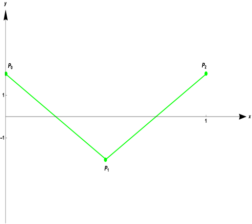
Figure 1: The fixed points $P_{0}$, $P_{1}$, $P_{2}$, and the graph $\Gamma_{{\cal W}_{0}}$, in the case where $\lambda=\displaystyle\frac{1}{2}$, and $N_{b}=3$.

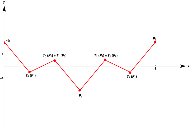
Figure 2: The graph $\Gamma_{{\cal W}_{1}}$, in the case where $\lambda=\displaystyle\frac{1}{2}$, and $N_{b}=3$. $T_{0}(P_{2})=T_{1}(P_{0})$ et $T_{1}(P_{2})=T_{2}(P_{1})$.

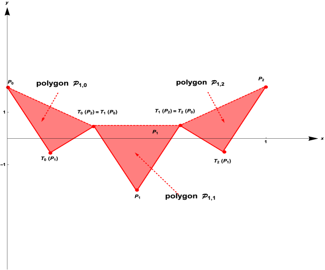
Figure 3: The polygons ${\cal P}_{1,0}$, ${\cal P}_{1,1}$, ${\cal P}_{1,2}$, in the case where $\lambda=\displaystyle\frac{1}{2}$, and $N_{b}=3$.

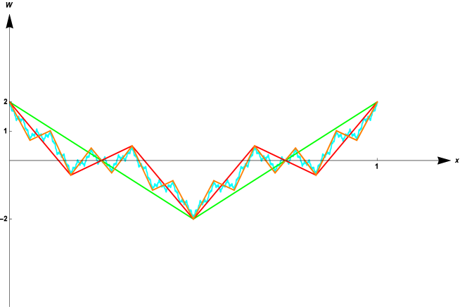
Figure 4: The graphs $\Gamma_{{\cal W}_{0}}$ (in green),  $\Gamma_{{\cal W}_{1}}$ (in red), $\Gamma_{{\cal W}_{2}}$ (in orange), $\Gamma_{{\cal W}}$ (in cyan), in the case where $\lambda=\displaystyle\frac{1}{2}$, and $N_{b}=3$.

Definition 2.2.

Consecutive vertices on the graph $\Gamma_{\cal W}$

Two points $X$ and $Y$ of $\Gamma_{{\cal W}}$ will be called consecutive vertices of the graph $\Gamma_{\cal W}$ if there exists a natural integer $m$, and an integer $j$ of $\left\{0,...,N_{b}-2\right\}$, such that:

$$X=\left(T_{i_{1}}\circ\ldots\circ T_{i_{m}}\right)(P_{j})\quad\text{and}\quad Y=\left(T_{i_{1}}\circ\ldots\circ T_{i_{m}}\right)(P_{j+1})\qquad\left\{i_{1},\ldots,i_{m}\right\}\,\in\,\left\{0,...,N_{b}-1\right\}^{m}$$

or:

$$X=\left(T_{i_{1}}\circ T_{i_{2}}\circ\ldots\circ T_{i_{m}}\right)\left(P_{N_{b}-1}\right)\quad\text{and}\quad Y=\left(T_{i_{1}+1}\circ T_{i_{2}}\ldots\circ T_{i_{m}}\right)(P_{0})$$

Remark 2.2.

It is important to note that $X$ and $Y$ cannot be in the same time the images of $P_{j}$ and $P_{j+1}$, $0\leqslant j\leqslant N_{b-2}$, by $T_{i_{1}}\circ\ldots\circ T_{i_{m}}$,  $(i_{1},\ldots,i_{m})\,\in\,\left\{0,...,N_{b}-2\right\}$, and of $P_{k}$ and $P_{k+1}$, $0\leqslant k\leqslant N_{b-2}$ ,
by $T_{p_{1}}\circ\ldots\circ T_{p_{m}}$, $(p_{1},\ldots,p_{m})\,\in\,\left\{0,...,N_{b}-2\right\}$. This result can be proved by induction, since, for any pair of integers $(j,k)$ of $\left\{0,...,N_{b}-2\right\}^{2}$ , for any $i_{m}$ of $\left\{0,...,N_{b}-2\right\}$, and any $p_{m}$ of $\left\{0,...,N_{b}-2\right\}$:

$$\left(i_{m}\neq p_{m}\quad\text{and}\quad j\neq k\right)\Longrightarrow\left(T_{i_{m}}\left(P_{j}\right)\neq T_{j_{m}}\left(P_{k}\right)\quad\text{and}\quad T_{i_{m}}\left(P_{j}\right)\neq T_{j_{m}}\left(P_{k}\right)\right)$$

Each contraction $T_{i}$, $0\leqslant i\leqslant N_{b}-1$ is indeed injective.

Since the vertices of the initial graph $\Gamma_{{\cal W}_{0}}$ are distinct, one gets the expected result.

Definition 2.3.

For any natural integer $m$, the ${\cal N}^{\cal S}_{m}$ consecutive vertices of the graph $\Gamma_{{\cal W}_{m}}$ are, also, the vertices of $N_{b}^{m}$ simple polygons ${\cal P}_{m,j}$, $0\leqslant j\leqslant N_{b}^{m}-1$, with $N_{b}$ sides. For any integer $j$ such that $0\leqslant j\leqslant N_{b}^{m}-1$, one obtains each polygon by linking the point number $j$ to the point number $j+1$ if $j=i\,\text{mod }N_{b}$, $0\leqslant i\leqslant N_{b}-2$, and the point number $j$ to the point number $j-N_{b}+1$ if $j=-1\,\text{mod }N_{b}$. These polygons generate a Borel set of ${\mathbb{R}}^{2}$.

Definition 2.4.

Polygonal domain delimited by the graph $\Gamma_{{\cal W}_{m}}$, $m\,\in\,{\mathbb{N}}$

For any natural integer $m$, well call polygonal domain delimited by the graph $\Gamma_{{\cal W}_{m}}$, and denote by ${\cal D}\left(\Gamma_{{\cal W}_{m}}\right)$, the reunion of the $N_{b}^{m}$ polygons ${\cal P}_{m,j}$, $0\leqslant j\leqslant N_{b}^{m}-1$, with $N_{b}$ sides.

Definition 2.5.

Polygonal domain delimited by the graph $\Gamma_{{\cal W}}$

We will call polygonal domain delimited by the graph $\Gamma_{{\cal W}}$, and denote by ${\cal D}\left(\Gamma_{{\cal W}}\right)$, the limit:

$${\cal D}\left(\Gamma_{{\cal W}}\right)=\displaystyle\lim_{m\to+\infty}{\cal D}\left(\Gamma_{{\cal W}_{m}}\right)$$

Definition 2.6.

Word, on the graph $\Gamma_{\cal W}$

Let $m$ be a strictly positive integer. We will call number-letter any integer ${\cal M}_{i}$ of $\left\{0,\ldots,N_{b}-1\right\}$, and word of length $|{\cal M}|=m$, on the graph $\Gamma_{\cal W}$, any set of number-letters of the form:

$${\cal M}=\left({\cal M}_{1},\ldots,{\cal M}_{m}\right)$$

We will write:

$$T_{\cal M}=T_{{\cal M}_{1}}\circ\ldots\circ T_{{\cal M}_{m}}$$

Property 2.7.

For any natural integer $m$ :

$$\Gamma_{\cal W}=\overline{\underset{|{\cal M}|=k\geqslant m}{\overset{}{\bigcup}}\,T_{\cal M}(\Gamma_{\cal W})}$$

Definition 2.7.

Edge relation, on the graph $\Gamma_{\cal W}$

Given a natural integer $m$, two points $X$ and $Y$ of $\Gamma_{{\cal W}_{m}}$ will be called adjacent if and only if $X$ and $Y$ are two consecutive vertices of $\Gamma_{{\cal W}_{m}}$. We will write:

$$X\underset{m}{\sim}Y$$

This edge relation ensures the existence of a word ${\cal M}=\left({\cal M}_{1},\ldots,{\cal M}_{m}\right)$ of length $m$, such that $X$ and $Y$ both belong to the iterate:

$$T_{\cal M}\,V_{0}=\left(T_{{\cal M}_{1}}\circ\ldots\circ T_{{\cal M}_{m}}\right)\,V_{0}$$

Given two points $X$ and $Y$ of the graph $\Gamma_{\cal W}$, we will say that $X$ and $Y$ are adjacent if and only if there exists a natural integer $m$ such that:

$$X\underset{m}{\sim}Y$$

Proposition 2.8.

Adresses, on the graph of the Weierstrass function

Given a strictly positive integer $m$, and a word ${\cal M}=\left({\cal M}_{1},\ldots,{\cal M}_{m}\right)$ of length $m\,\in\,{\mathbb{N}}^{\star}$, on the graph $\Gamma_{{\cal W}_{m}}$, for any integer $j$ of $\left\{1,...,N_{b}-2\right\}$, any $X=T_{\cal M}(P_{j})$ of $V_{m}\setminus V_{0}$, i.e. distinct from one of the $N_{b}$ fixed point $P_{i}$,  $0\leqslant i\leqslant N_{b}-1$, has exactly two adjacent vertices, given by:

$$T_{\cal M}(P_{j+1})\quad\text{and}\quad T_{\cal M}(P_{j-1})$$

where:

$$T_{\cal M}=T_{{\cal M}_{1}}\circ\ldots\circ T_{{\cal M}_{m}}$$

By convention, the adjacent vertices of $T_{{\cal M}}(P_{0})$ are $T_{{\cal M}}(P_{1})$ and $T_{{\cal M}}(P_{N_{b}-1})$, those of $T_{{\cal M}}(P_{N_{b}-1})$, $T_{{\cal M}}(P_{N_{b}-2})$ and $T_{{\cal M}}(P_{0})$ .

Property 2.9.

The set of vertices $\left(V_{m}\right)_{m\in{\mathbb{N}}}$ is dense in $\Gamma_{{\cal W}}$.

Definition 2.8.

Power of a vertex of the graph $\Gamma_{{\mathcal{W}}_{m}}$, $m\,\in\,{\mathbb{N}}^{\star}$

Given a strictly positive integer $m$, a vertex $X$ of the graph $\Gamma_{{\mathcal{W}}_{m}}$ will be said of power one if $X$ belongs to one and only one $N_{b}$-gon ${\cal P}_{m,j}$, $0\leqslant j\leqslant N_{b}^{m}-1$, and of power $\displaystyle\frac{1}{2}$ if $X$ is a common vertex to consecutive $N_{b}$-gons ${\cal P}_{m,j}$ and ${\cal P}_{m,j^{\prime}}$, $0\leqslant j\leqslant N_{b}^{m}-1$, $0\leqslant j^{\prime}\leqslant N_{b}^{m}-1$, $j^{\prime}\neq j$.
In the sequel, the power of the vertex $X$ will be denoted by:

$$p(X)$$

Definition 2.9.

Measure, on the domain delimited by the graph $\Gamma_{{\cal W}}$

We will call domain delimited by the graph $\Gamma_{{\cal W}}$, and denote by ${\cal D}\left(\Gamma_{{\cal W}}\right)$, the limit:

$${\cal D}\left(\Gamma_{{\cal W}}\right)=\displaystyle\lim_{n\to+\infty}{\cal D}\left(\Gamma_{{\cal W}_{m}}\right)$$

which has to be understood in the following way: given a continuous function $u$ on the graph $\Gamma_{\cal W}$, and a measure with full support $\mu$ on ${\mathbb{R}}^{2}$, then:

$$\int_{{\cal D}\left(\Gamma_{{\cal W}}\right)}u\,d\mu=\displaystyle\lim_{m\to+\infty}\displaystyle\sum_{j=0}^{N_{b}^{m}-1}\displaystyle\sum_{X\,\text{vertex of }{\cal P}_{m,j}}\frac{p\left(X\right)\,u\left(X\right)\,\mu\left({\cal P}_{m,j}\right)}{N_{b}}$$

We will say that $\mu$ is a measure, on the domain delimited by the graph $\Gamma_{{\cal W}}$.

Definition 2.10.

Dirichlet form (we refer to the paper [BD85], or the book [FOT94])

Given a measured space $(E,\mu)$, a Dirichlet form on $E$ is a bilinear symmetric form, that we will denote by ${\cal E}$, defined on a vectorial subspace $D$ dense in $L^{2}(E,\mu)$, such that:

1. For any real-valued function $u$ defined on $D$ : ${\cal E}(u,u)\geqslant 0$.

2. $D$, equipped with the inner product which, to any pair $(u,v)$ of $D\times D$, associates:

   $$(u,v)_{\cal{E}}=(u,v)_{L^{2}(E,\mu)}+{\cal{E}}(u,v)$$

   is a Hilbert space.

3. For any real-valued function $u$ defined on $D$, if:

   $$u_{\star}=\min\,(\max(u,0),1)\,\in\,D$$

   then : ${\cal{E}}(u_{\star},u_{\star})\leqslant{\cal{E}}(u,u)$ (Markov property, or lack of memory property).

Definition 2.11.

Dirichlet form, on a finite set ([Kig03])

Let $V$ denote a finite set $V$, equipped with the usual inner product which, to any pair $(u,v)$ of functions defined on $V$, associates:

$$(u,v)=\displaystyle\sum_{p\in V}u(p)\,v(p)$$

A Dirichlet form on $V$ is a symmetric bilinear form ${\cal E}$, such that:

1. For any real valued function $u$ defined on $V$: ${\cal E}(u,u)\geqslant 0$.

2. ${\cal{E}}(u,u)=0$ if and only if $u$ is constant on $V$.

3. For any real-valued function $u$ defined on $V$, if:

   $$u_{\star}=\min\,(\max(u,0),1)$$

   i.e. :

   $$\forall\,p\,\in\,V\,:\quad u_{\star}(p)=\left\{\begin{array}[]{ccc}1&\text{if}&u(p)\geqslant 1\\ u(p)&\text{si}&0<u(p)<1\\ 0&\text{if}&u(p)\leqslant 0\end{array}\right.$$

   then: ${\cal{E}}(u_{\star},u_{\star})\leqslant{\cal{E}}(u,u)$ (Markov property).

Remark 2.3.

In order to understand the underlying theory of Dirichlet forms, one can only refer to the work of A. Beurling and J. Deny [BD85]. The Dirichlet space $\cal D$ of fonctions $u$, complex valued functions, infinitely differentiable, the support of which belongs to a domain $\omega\subset{\mathbb{R}}^{p}$, $p\,\in\,{\mathbb{N}}^{\star}$, is equipped with the hilbertian norm:

$$u\mapsto\|u\|_{\cal D}=\displaystyle\int_{\omega}|\text{grad}\,u(x)|^{2}\,dx$$

If the complement set of $\omega$ is not "too small", the space $\cal D$ can be completed by adding functions defined almost everywhere in $\omega$. The space thus obtained ${\cal D}_{\omega}$, equipped with the Lebesgue measure $\xi$, satisfies the following properties:

1. For any compact $K\subset\omega$, there exists a positive constant $C_{K}$ such that, for any $u$ of ${\cal D}_{\omega}$:

   $$\int_{K}|u(x)|\,d\xi(x)\leqslant C_{K}\,\|u\|_{{\cal D}_{\omega}}$$

2. If one denotes by $\cal C$ the space of complex-valued, continuous functions with compact support, then: ${\cal C}\cap{\cal D}_{\omega}$ is dense in $\cal C$ and in ${\cal D}_{\omega}$.

3. For any contraction of the complex plane, and any $u$ of ${\cal D}_{\omega}$:

   $$T\,u\,\in\,{\cal D}_{\omega}\quad\text{and}\quad\|T\,u\|_{{\cal D}_{\omega}}\leqslant\|u\|_{{\cal D}_{\omega}}$$

The Dirichlet space ${\cal D}_{\omega}$ is generated by the Green potentials of finite energy, which are defined in a direct way, as the functions $u$ of ${\cal D}_{\omega}$ such that there exists a Radon measure $\mu$ such that:

$$\forall\,\varphi\,\in\,{\cal C}\cap{\cal D}_{\omega}\,:\quad\left(u,\varphi\right)=\displaystyle\int_{\omega}\bar{\varphi}\,d\mu$$

Such a map $u$ will be called potential generated by $\mu$.

The linear map $\Delta$ which, to any potential $u$ of ${\cal D}_{\omega}$, associates the measure $\mu$ that generates this potential, is called generalized Laplacian for the space ${\cal D}$.

It is interesting to note that the original theory of Dirichlet spaces concerned functions defined on a Hausdorff space (separated espace ), with a positive Radon measure of full support (every non-empty open set has a strictly positive measure).

Remark 2.4.

One may wonder why the Markov property is of such importance in our building of a Laplacian ? Very simply, the lack of memory - or the fact that the future state which corresponds, for any natural integer $m$, to the values of the considered function on the graph $\Gamma_{{\cal W}_{m+1}}$, depends only of the present state, i.e. the values of the function on the graph $\Gamma_{{\cal W}_{m}}$, accounts for the building of the Laplacian step by step.

Theorem 2.10.

An upper bound and a lower bound, for the box-dimension of the graph $\Gamma_{\mathcal{W}}$

For any integer $j$ belonging to $\left\{0,1,\ldots,N_{b}-2\right\}$, each natural integer $m$, and each word $\mathcal{M}$ of length $m$, let us consider the rectangle, whose sides are parallel to the horizontal and vertical axes, of width:

$$L_{m}=x\left(T_{\mathcal{M}}\left(P_{j+1}\right)\right)-x\left(T_{\mathcal{M}}\left(P_{j}\right)\right)=\displaystyle\frac{1}{(N_{b}-1)\,N_{b}^{m}}$$

and height $|h_{j,m}|$, such that the points $T_{\mathcal{M}}\left(P_{j}\right)$ and $T_{\mathcal{M}}\left(P_{j+1}\right)$ are two vertices of this rectangle.
Then:

i. When the integer $N_{b}$ is odd:

$$L_{m}^{2-D_{\mathcal{W}}}\,(N_{b}-1)^{2-D_{\mathcal{W}}}\,\left\{\displaystyle\frac{2}{1-\lambda}\,\sin\left(\displaystyle\frac{\pi}{N_{b}-1}\right)\displaystyle\min_{0\leqslant j\leqslant N_{b}-1}\left|\sin\left(\displaystyle\frac{\pi\,(2\,j+1)}{N_{b}-1}\right)\right|-\displaystyle\frac{2\,\pi}{N_{b}\,(N_{b}-1)}\,\displaystyle\frac{1}{\lambda\,N_{b}-1}\right\}\leqslant|h_{j,m}|$$

ii. When the integer $N_{b}$ is even:

$$L_{m}^{2-D_{\mathcal{W}}}(N_{b}-1)^{2-D_{\mathcal{W}}}\max\left\{\!\!\displaystyle\frac{2}{1-\lambda}\sin\left(\displaystyle\frac{\pi}{N_{b}-1}\right)\!\!\displaystyle\min_{0\leqslant j\leqslant N_{b}-1}\!\!\left|\sin\left(\displaystyle\frac{\pi\,(2\,j+1)}{N_{b}-1}\right)\right|\!\!-\!\!\displaystyle\frac{2\,\pi}{N_{b}\,(N_{b}-1)}\displaystyle\frac{1}{\lambda\,N_{b}-1},\displaystyle\frac{4}{N_{b}^{2}}\displaystyle\frac{1-N_{b}^{-2}}{N_{b}^{2}-1}\right\}\!\!\leqslant\!|h_{j,m}|\!$$

Also:

$$|h_{j,m}|\leqslant\eta_{{\mathcal{W}}}\,L_{m}^{2-D_{\mathcal{W}}}\,(N_{b}-1)^{2-D_{\mathcal{W}}}\,$$

where the real constant $\eta_{{\mathcal{W}}}$ is given by :

$$\eta_{{\mathcal{W}}}=2\,\pi^{2}\,\left\{\displaystyle\frac{(2\,N_{b}-1)\,\lambda\,(N_{b}^{2}-1)}{(N_{b}-1)^{2}\,(1-\lambda)\,(\lambda\,N_{b}^{2}-1)}+\displaystyle\frac{2\,N_{b}}{(\lambda\,N_{b}^{2}-1)\,(\lambda\,N_{b}^{3}-1)}\right\}.$$

Notation.

In the sequel, we set, for any natural integer $m$:

$$h_{m}=L_{m}^{2-D_{\mathcal{W}}}=\displaystyle\frac{N_{b}^{(D_{\mathcal{W}}-2)\,m}}{(N_{b}-1)^{2-D_{\mathcal{W}}}}$$

and:

$$h=N_{b}^{(D_{\mathcal{W}}-2)}$$

Definition 2.12.

Energy, on the graph $\Gamma_{{\cal W}_{m}}$, $m\,\in\,{\mathbb{N}}$, of a pair of functions

Let $m$ be a natural integer, and $u$ and $v$ two real valued functions, defined on the set

$$V_{m}=\left\{{\cal S}_{0}^{m},{\cal S}_{1}^{m},\ldots,{\cal S}_{{\cal N}_{m}^{\cal S}-1}^{m}\right\}$$

of the ${\cal N}_{m}^{\cal S}$ vertices of $\Gamma_{{\cal W}_{m}}$.

It appears as natural to introduce the energy, on the graph $\Gamma_{{\cal W}_{m}}$, of the pair of functions $(u,v)$, as:

$$\begin{array}[]{ccc}{\cal{E}}_{\Gamma_{{\cal W}_{m}}}(u,v)&=&\displaystyle\sum_{i=0}^{{\cal N}_{m}^{\cal S}-2}\left(\displaystyle\frac{u\left({\cal S}_{i}^{m}\right)-u\left({\cal S}_{i+1}^{m}\right)}{h_{m}}\right)\,\left(\displaystyle\frac{v\left({\cal S}_{i}^{m}\right)-v\left({\cal S}_{i+1}^{m}\right)}{h_{m}}\right)\end{array}$$

For the sake of simplicity, we will write it under the form:

$${\cal{E}}_{\Gamma_{{\cal W}_{m}}}(u,v)=\displaystyle\frac{1}{h_{m}^{2}}\,\displaystyle\sum_{X\underset{m}{\sim}Y}\left(u(X)-u(Y)\right)\,\left(v(X)-v(Y)\right)$$

Property 2.11.

Given a natural integer $m$, and a real-valued function $u$, defined on the set of vertices of $\Gamma_{{\cal W}_{m}}$, the map, which, to any pair of real-valued, continuous functions $(u,v)$ defined on the set $V_{m}$ of the ${\cal N}_{m}$ vertices of $\Gamma_{{\cal W}_{m}}$, associates:

$${\cal{E}}_{\Gamma_{{\cal W}_{m}}}(u,v)=\displaystyle\frac{1}{h_{m}^{2}}\,\displaystyle\sum_{X\underset{m}{\sim}Y}\left(u(X)-u(Y)\right)\,\left(v(X)-v(Y)\right)$$

is a Dirichlet form on $\Gamma_{{\cal W}_{m}}$.
Moreover:

$${\cal{E}}_{\Gamma_{{\cal W}_{m}}}(u,u)=0\Leftrightarrow u\text{ is constant}$$

Proposition 2.12.

Harmonic extension of a function, on the graph of the Weierstrass function

For any strictly positive integer $m$, if $u$ is a real-valued function defined on $V_{m-1}$, its harmonic extension, denoted by $\tilde{u}$, is obtained as the extension of $u$ to $V_{m}$ which minimizes the energy:

$${\cal{E}}_{\Gamma_{{\cal W}_{m}}}(\tilde{u},\tilde{u})=\displaystyle\sum_{X\underset{m}{\sim}Y}\displaystyle\frac{(\tilde{u}(X)-\tilde{u}(Y))^{2}}{h_{m}^{2}}$$

The link between ${\cal{E}}_{\Gamma_{{\cal W}_{m}}}$ and ${\cal{E}}_{\Gamma_{{\cal W}_{m-1}}}$ is obtained through the introduction of two strictly positive constants $r_{m}$ and $r_{m-1}$ such that:

$$r_{m}\,\displaystyle\sum_{X\underset{m}{\sim}Y}\displaystyle\frac{(\tilde{u}(X)-\tilde{u}(Y))^{2}}{h_{m}}=\displaystyle\frac{r_{m-1}}{h^{2}}\,\displaystyle\sum_{X\underset{m-1}{\sim}Y}\displaystyle\frac{(u(X)-u(Y))^{2}}{h_{m-1}^{2}}$$

In particular:

$$r_{1}\,\displaystyle\sum_{X\underset{1}{\sim}Y}(\tilde{u}(X)-\tilde{u}(Y))^{2}=r_{0}\,\displaystyle\sum_{X\underset{0}{\sim}Y}(u(X)-u(Y))^{2}$$

For the sake of simplicity, we will fix the value of the initial constant: $r_{0}=1$. One has then:

$${\cal{E}}_{\Gamma_{{\cal W}_{1}}}(\tilde{u},\tilde{u})=\displaystyle\frac{1}{r_{1}\,h^{2}}\,{\cal{E}}_{\Gamma_{{\cal W}_{0}}}(\tilde{u},\tilde{u})$$

Let us set:

$$r=\displaystyle\frac{1}{r_{1}}$$

and:

$${\cal{E}}_{m}(u)=r_{m}\,\sum_{X\underset{m}{\sim}Y}\displaystyle\frac{(\tilde{u}(X)-\tilde{u}(Y))^{2}}{h_{m}^{2}}$$

Since the determination of the harmonic extension of a function appears to be a local problem, on the graph $\Gamma_{{\cal W}_{m-1}}$, which is linked to the graph $\Gamma_{{\cal W}_{m}}$ by a similar process as the one that links $\Gamma_{{\cal W}_{1}}$ to $\Gamma_{{\cal W}_{0}}$, one deduces, for any strictly positive integer $m$:

$${\cal{E}}_{\Gamma_{{\cal W}_{m}}}(\tilde{u},\tilde{u})=\displaystyle\frac{1}{r_{1}}\,{\cal{E}}_{\Gamma_{{\cal W}_{m-1}}}(\tilde{u},\tilde{u})$$

By induction, one gets:

$$r_{m}=r_{1}^{m}\,r_{0}=r^{-m}=N_{b}^{m}$$

If $v$ is a real-valued function, defined on $V_{m-1}$, of harmonic extension $\tilde{v}$, we will write:

$${\cal{E}}_{m}(u,v)=r^{-m}\,\sum_{X\underset{m}{\sim}Y}\displaystyle\frac{(\tilde{u}(X)-\tilde{u}(Y))\,(\tilde{v}(X)-\tilde{v}(Y))}{h_{m}^{2}}$$

For further precision on the construction and existence of harmonic extensions, we refer to [Sab97].

Nota Bene:

The above latter energy formula writes:

$${\cal{E}}_{m}(u,u)=N_{b}^{(5-2\,D_{\mathcal{W}})\,m}\,\sum_{X\underset{m}{\sim}Y}\left(\tilde{u}(X)-\tilde{u}(Y)\right)^{2}$$

We would like to lay the emphazis upon the fact that this work involves a mixt approach, using both the methods of J. Kigami and R. S. Strichartz, and the one by U. Mosco for fractal curves [Mos02], which takes into account topology and geometry, by the means of a quasi-distance, built from the eucidean one $d_{eucl}$ between adjacent points $X$ and $Y$ such that ${X\underset{m}{\sim}Y}$ :

$$d(X,Y)=\left(d_{eucl}(X,Y)\right)^{\delta}$$

where $\delta$ is a real constant. The related energy writes:

$${\cal{E}}_{m}(u)=\sum_{X\underset{m}{\sim}Y}\displaystyle\frac{(\tilde{u}(X)-\tilde{u}(Y))^{2}}{d^{2}(X,Y)}$$

Yet, one cannot apply this method in our case, the constant $\delta$ being a priori determined, either by decimation, either in order to verify the Gaussian principle. It is impossible to determine this constant in a non-affine framework like that of the graph of the Weierstrass function.

The question one may ask is wether one may be sure that $N_{b}^{(5-2\,D_{\mathcal{W}})\,m}$ is the right constant in the present case ? The question is not an inocuous one, in so far as the value of this constant directly affects the spectra of the related Laplacian.

The point is that, by construction, our energies satisfy the maximum principle. Also, the value of this constant joins the one at stake in the value of the population spectral density of fractional Brown functions evoked in [Man77a]. It is obtained The links between randomized forms of the Weierstrass functions and fractional Brownian motion incline us to think that we are in the good direction.

Notation.

Given a strictly positive integer $m$, let us consider a vertex $X$ of the graph ${\Gamma}_{{\cal W}_{m}}$. Two configurations can occur:

1. the vertex $X$ belongs to one and only one polygon with $N_{b}$ sides, ${\cal P}_{m,j}$, $0\leqslant j\leqslant N_{b}^{m}-1$. We set:

   $${\cal A}_{m}=\mu\left({\cal P}_{m,j}\right)$$

2. the vertex $X$ is the intersection point of two polygons with $N_{b}$ sides, ${\cal P}_{m,j}$ and ${\cal P}_{m,j+1}$, $0\leqslant j\leqslant N_{b}^{m}-2$. We set:

   $${\cal A}_{m}=\displaystyle\frac{1}{2}\,\left\{\mu\left({\cal P}_{m,j}\right)+\mu\left({\cal P}_{m,j+1}\right)\right\}$$

Definition 2.13.

Dirichlet form, for a pair of continuous functions defined on the graph $\Gamma_{{\cal W}}$

We define the Dirichlet form $\cal{E}$ which, to any pair of real-valued, continuous functions $(u,v)$ defined on the graph $\Gamma_{{\cal W}}$, associates, subject to its existence:

$${\cal{E}}(u,v)=\displaystyle\lim_{m\to+\infty}\displaystyle\sum_{X\underset{m}{\sim}Y}r^{-m}\,\displaystyle\frac{\left(u_{\mid V_{m}}(X)-u_{\mid V_{m}}(Y)\right)\,\left(v_{\mid V_{m}}(X)-v_{\mid V_{m}}(Y)\right)}{h_{m}^{2}}\,\frac{{\cal A}_{m}}{N_{b}}$$

Definition 2.14.

Normalized energy, for a continuous function $u$, defined on the graph $\Gamma_{{\cal W}}$
Taking into account that the sequence $\left(\mathcal{E}_{m}\left(u_{\mid V_{m}}\right)\right)_{m\in{\mathbb{N}}}$ is defined on

$${V_{\star}=\underset{{i\in{\mathbb{N}}}}{\bigcup}\,V_{i}}$$

one defines the normalized energy, for a continuous function $u$, defined on the graph $\Gamma_{{\cal W}}$, by:

$${\cal{E}}(u)=\displaystyle\lim_{m\to+\infty}\displaystyle\sum_{X\underset{m}{\sim}Y}r^{-m}\,\displaystyle\frac{\left(u_{\mid V_{m}}(X)-u_{\mid V_{m}}(Y)\right)^{2}}{h_{m}^{2}}\,\frac{{\cal A}_{m}}{N_{b}}$$

Notation.

We will denote by $\text{dom}\,{\cal E}$ the subspace of continuous functions defined on $\Gamma_{\cal W}$, such that:

$$\mathcal{E}(u)<+\infty$$

Notation.

We will denote by $\text{dom}_{0}\,{\cal E}$ the subspace of continuous functions defined on $\Gamma_{\cal W}$, which take the value on $V_{0}$, such that:

$$\mathcal{E}(u)<+\infty$$

3 Laplacian of a continuous function, on the graph of the Weierstrass function

3.1 Theoretical aspect

Property 3.1.

Building of a specific measure, for the domain delimited by the graph of the Weierstrass function

The Dirichlet forms mentioned in the above require a positive Radon measure with full support. In auto-affine configurations (the Sierpiński Gasket for instance), the choice of a self-similar measure, which is, mots of the time, built with regards to a reference set, of measure 1, appears, first, as very natural. More generally, R. S. Strichartz [RSS95], [Str99], showed that one can simply consider auto-replicant measures $\tilde{\mu}$, i.e. measures $\mu$ such that:

$$\mu=\displaystyle\sum_{i=0}^{N_{b}-1}\mu_{i}\,\mu\circ T_{i}^{-1}\qquad(\star)$$

where $\left(\mu_{i}\right)_{0\leqslant i\leqslant N_{b}-1}$ denotes a family of strictly positive pounds.

The non-affine framework makes it clear that there cannot exist such constant coefficients $\mu_{i}$. It appears more realistic that they depend on the order $m\,\in\,{\mathbb{N}}^{\star}$ of the iteration, as:

$$\mu=\displaystyle\sum_{i=0}^{N_{b}-1}\mu_{m,i}\,\mu\circ T_{i}^{-1}\qquad(\star_{m})$$

Let us thus denote by $\mu_{\cal L}$ the Lebesgue measure on ${\mathbb{R}}^{2}$, and start with the normalized measure:

$$\mu=\displaystyle\frac{\mu_{\cal L}}{\mu_{\cal L}\left({\cal P}_{0}\right)}$$

and look for a family of strictly positive pounds $\left(\mu_{1,i}\right)_{0\leqslant i\leqslant N_{b}-1}$ such that:

$$\mu\left(T_{0}\left({\cal P}_{0}\right)\cup T_{1}\left({\cal P}_{0}\right)\cup T_{2}\left({\cal P}_{0}\right)\cup\ldots\cup T_{N_{b}-1}\left({\cal P}_{0}\right)\right)=\displaystyle\sum_{i=0}^{N_{b}-1}\mu_{1,i}\,{\mu}\left({\cal P}_{0}\right)=\displaystyle\sum_{i=0}^{N_{b}-1}\mu_{1,i}$$

The convenient choice, for any $i$ of $\left\{0,\ldots,N_{b}-1\right\}$, is:

$$\mu_{1,i}=\mu\left(T_{i}\left({\cal P}_{0}\right)\right)$$

Now, given a strictly positive integer $m$, let us look for a family of strictly positive pounds $\left(\mu_{1,i}\right)_{0\leqslant i\leqslant N_{b}-1}$ such that:

$$\mu=\displaystyle\sum_{i=0}^{N_{b}-1}\mu_{m,i}\,\mu_{0}\circ T_{i}^{-1}\qquad(\star_{m})$$

where $\left(\mu_{m,i}\right)_{0\leqslant i\leqslant N_{b}-1}$ denotes a family of strictly positive pounds.

Relation $(\star_{m})$ yields, for any set of polygons ${\cal P}_{m,j}$, $m\,\in\,{\mathbb{N}}$, $0\leqslant j\leqslant N_{b}^{m}-1$, with $N_{b}$ sides:

$$\mu\left(\underset{0\leqslant j\leqslant N_{b}^{m}-1}{\bigcup}{\cal P}_{m,j}\right)=\displaystyle\sum_{i=0}^{N_{b}-1}\mu_{m,i}\,\mu\left(\left(\underset{0\leqslant j\leqslant N_{b}^{m-1}-1}{\bigcup}{\cal P}_{m-1,j}\right)\right)$$

and, in particular:

$$\mu\left(T_{0}\left(\underset{0\leqslant j\leqslant N_{b}^{m-1}-1}{\bigcup}{\cal P}_{m-1,j}\right)\cup\ldots\cup T_{N_{b}-1}\left(\underset{0\leqslant j\leqslant N_{b}^{m-1}-1}{\bigcup}{\cal P}_{m-1,j}\right)\right)=\displaystyle\sum_{i=0}^{N_{b}-1}\mu_{m,i}\,\mu\left(\underset{0\leqslant j\leqslant N_{b}^{m-1}-1}{\bigcup}{\cal P}_{m-1,j}\right)$$

i.e.:

$$\sum_{i=0}^{N_{b}-1}\mu\left(T_{i}\left(\underset{0\leqslant j\leqslant N_{b}^{m-1}-1}{\bigcup}{\cal P}_{m-1,j}\right)\right)=\displaystyle\sum_{i=0}^{N_{b}-1}\mu_{i}\,\mu\left(\underset{0\leqslant j\leqslant N_{b}^{m-1}-1}{\bigcup}{\cal P}_{m-1,j}\right)$$

The convenient choice, for any $i$ of $\left\{0,\ldots,N_{b}-1\right\}$ , is:

$$\mu_{m,i}=\displaystyle\frac{\mu_{0}\left(T_{i}\left(\underset{0\leqslant j\leqslant N_{b}^{m-1}-1}{\bigcup}{\cal P}_{m-1,j}\right)\right)}{\mu\left(\underset{0\leqslant j\leqslant N_{b}^{m-1}-1}{\bigcup}{\cal P}_{m-1,j}\right)}$$

Remark 3.1.

The above result appears as as interesting splitting, fitted for the polygonal domain ${\cal D}\left(\Gamma_{{\cal W}}\right)$.

Definition 3.1.

Laplacian of order $m\,\in\,{\mathbb{N}}^{\star}$

For any strictly positive integer $m$, and any real-valued function $u$, defined on the set $V_{m}$ of the vertices of the graph $\Gamma_{{\cal W}_{m}}$, we introduce the Laplacian of order $m$, $\Delta_{m}(u)$, by:

$$\Delta_{m}u(X)=\displaystyle\frac{1}{h_{m}^{2}}\,\displaystyle\sum_{Y\in V_{m},\,Y\underset{m}{\sim}X}\left(u(Y)-u(X)\right)\quad\forall\,X\,\in\,V_{m}\setminus V_{0}$$

Definition 3.2.

Harmonic function of order $m\,\in\,{\mathbb{N}}^{\star}$

Let $m$ be a strictly positive integer. A real-valued function $u$,defined on the set $V_{m}$ of the vertices of the graph $\Gamma_{{\cal W}_{m}}$, will be said to be harmonic of order $m$ if its Laplacian of order $m$ is null:

$$\Delta_{m}u(X)=0\quad\forall\,X\,\in\,V_{m}\setminus V_{0}$$

Definition 3.3.

Piecewise harmonic function of order $m\,\in\,{\mathbb{N}}^{\star}$

Given a strictly positive integer $m$, a real valued function $u$, defined on the set of vertices of $\Gamma_{\cal W}$, is said to be piecewise harmonic function of order $m$ if, for any word ${\cal M}$ of length $m$, $u\circ T_{\cal M}$ is harmonic of order $m$.

Definition 3.4.

Existence domain of the Laplacian, for a continuous function on the graph $\Gamma_{\cal W}$ (see [BD85])

We will denote by $\text{dom}\,\Delta$ the existence domain of the Laplacian, on the graph $\Gamma_{\cal W}$, as the set of functions $u$ of $\text{dom}\,\mathcal{E}$ such that there exists a continuous function on $\Gamma_{\cal W}$, denoted $\Delta\,u$, that we will call Laplacian of $u$, such that :

$$\mathcal{E}(u,v)=-\displaystyle\int_{{\cal D}\left(\Gamma_{\cal W}\right)}v\,\Delta u\,d\mu\quad\text{for any }v\,\in\,\text{dom}_{0}\,\mathcal{E}$$

Definition 3.5.

Harmonic function

A function $u$ belonging to $\text{dom}\,\Delta$ will be said to be harmonic if its Laplacian is equal to zero.

Notation.

In the following, we will denote by ${\cal H}_{0}\subset\text{dom}\,\Delta$ the space of harmonic functions, i.e. the space of functions $u\,\in\,\ \text{dom}\,\Delta$ such that:

$$\Delta\,u=0$$

Given a natural integer $m$, we will denote by ${\cal S}\left({\cal H}_{0},V_{m}\right)$ the space, of dimension $N_{b}^{m}$, of spline functions " of level $m$",  $u$, defined on $\Gamma_{\cal W}$, continuous, such that, for any word $\cal M$ of length $m$, $u\circ T_{\cal M}$ is harmonic, i.e.:

$$\Delta_{m}\,\left(u\circ T_{\cal M}\right)=0$$

Property 3.2.

For any natural integer $m$:

$${\cal S}\left({\cal H}_{0},V_{m}\right)\subset\text{dom }{\cal E}$$

3.2 Explicit determination of the Laplacian of a function $u$ of $\text{dom}\,\Delta$

Definition 3.6.

Spline functions on ${\cal D}\left(\Gamma_{{\cal W}_{m}}\right)$, $m\,\in\,{\mathbb{N}}^{\star}$

Given a strictly positive integer $m$, let us consider a vertex $X$ of the graph ${\Gamma}_{{\cal W}_{m}}$. Two configurations can occur:

1. the vertex $X$ belongs to one and only one polygon with $N_{b}$ sides, ${\cal P}_{m,j}$, $0\leqslant j\leqslant N_{b}^{m}-1$.
   

   In this case, if one considers the spline functions $\psi_{Z}^{m}$ which correspond to the $N_{b}-1$ vertices of this polygon distinct from $X$:

   $$\sum_{Z\,\text{vertex of~{}${\cal P}_{m,j}$}}\displaystyle\int_{{\cal D}\left(\Gamma_{\cal W}\right)}\psi_{Z}^{m}\,d\mu=\mu\left({\cal P}_{m,j}\right)$$

   i.e., by symmetry:

   $$N_{b}\,\displaystyle\int_{{\cal D}\left(\Gamma_{\cal W}\right)}\psi_{X}^{m}\,d\mu=\mu\left({\cal P}_{m,j}\right)$$

   Thus:

   $$\int_{{\cal D}\left(\Gamma_{\cal W}\right)}\psi_{X}^{m}\,d\mu=\displaystyle\frac{1}{N_{b}}\,\mu\left({\cal P}_{m,j}\right)=\frac{{\cal A}_{m}}{N_{b}}$$

   where we retrieve the quantities ${\cal A}_{m}$ of definition Notation.

   
   

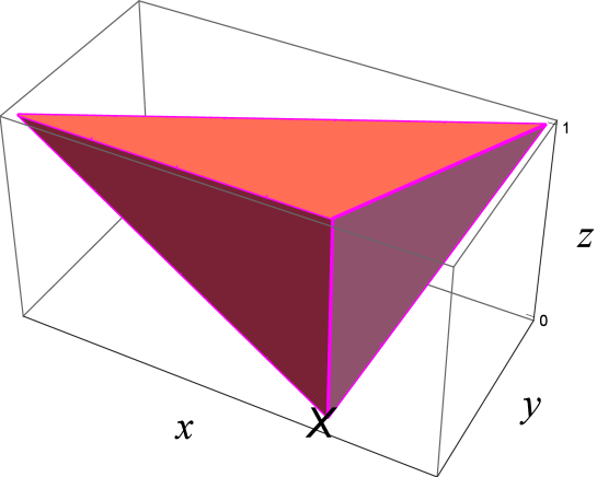
   Figure 5: The graph of a spline function $\psi_{X}^{m}$, $m\,\in\,{\mathbb{N}}$, in the case $N_{b}=3$.

   
   

2. the vertex $X$ is the intersection point of two polygons with $N_{b}$ sides, ${\cal P}_{m,j}$ and ${\cal P}_{m,j+1}$, $0\leqslant j\leqslant N_{b}^{m}-2$.
   

   On has then to take into account the contributions of both polygons, which leads to:

   $$\int_{{\cal D}\left(\Gamma_{\cal W}\right)}\psi_{X}^{m}\,d\mu=\displaystyle\frac{1}{2\,N_{b}}\,\left\{\mu\left({\cal P}_{m,j}\right)+\mu\left({\cal P}_{m,j+1}\right)\right\}=\frac{{\cal A}_{m}}{N_{b}}$$

   where, again, we retrieve the quantities ${\cal A}_{m}$ of definition Notation.

Remark 3.2.

As it is explained in [Str06], one has just to reason by analogy with the dimension 1, more particulary, the unit interval $I=[0,1]$, of extremities $X_{0}=(0,0)$, and $X_{1}=(1,0)$. The functions $\psi_{X_{1}}$ and $\psi_{X_{2}}$ such that, for any $Y$ of ${\mathbb{R}}^{2}$ :

$$\psi_{X_{1}}(Y)=\delta_{X_{1}Y}\quad,\quad\psi_{X_{2}}(Y)=\delta_{X_{2}Y}$$

are, in the most simple way, tent functions. For the standard measure, one gets values that do not depend on $X_{1}$, or $X_{2}$ (one could, also, choose to fix $X_{1}$ and $X_{2}$ in the interior of $I$) :

$$\int_{I}\psi_{X_{1}}\,d\mu=\displaystyle\int_{I}\psi_{X_{2}}\,d\mu=\displaystyle\frac{1}{2}$$

(which corresponds to the surfaces of the two tent triangles.)

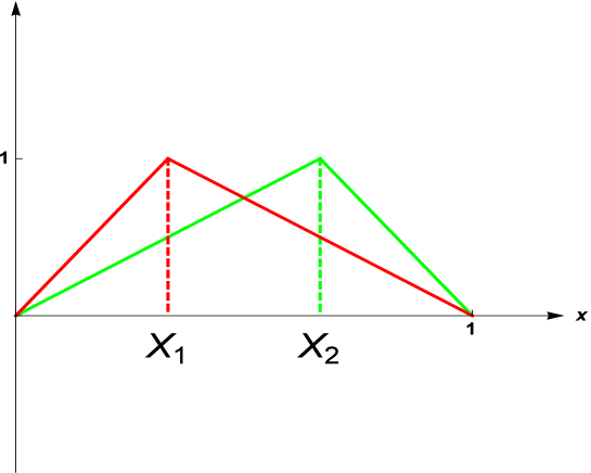
Figure 6: The graphs of the spline functions $\psi_{X_{1}}$ and $\psi_{X_{2}}$.

In our case, we have just build the pendant, by no longer reasoning on the unit interval, but on our $N_{b}$-gons.

Property 3.3.

Let $m$ be a strictly positive integer, $X\,\notin\,V_{0}$ a vertex of the graph $\Gamma_{\cal W}$, and $\psi_{X}^{m}\,\in\,{\cal S}\left({\cal H}_{0},V_{m}\right)$ a spline function such that:

$$\psi_{X}^{m}(Y)=\left\{\begin{array}[]{ccc}\delta_{XY}&\forall&Y\,\in\,V_{m}\\ 0&\forall&Y\,\notin\,V_{m}\end{array}\right.\quad,\quad\text{where}\quad\delta_{XY}=\left\{\begin{array}[]{ccc}1&\text{if}&X=Y\\ 0&\text{else}&\end{array}\right.$$

Then, since $X\,\notin\,V_{0}$: $\psi_{X}^{m}\,\in\,\text{dom}_{0}\,\mathcal{E}$.

Let us first note that:

$$\begin{array}[]{ccc}{\cal E}\left(u,\psi_{X}^{m}\right)&=&\displaystyle\sum_{Y\in V_{m},\,Y\underset{m}{\sim}X}\Delta_{m}u(X)\,\left(\psi_{X}^{m}(Y)(Y)-\psi_{X}^{m}(Y)\right)\,\left(\displaystyle\int_{{\cal D}\left(\Gamma_{\cal W}\right)}\psi_{X}^{m}\,d\mu\right)\\ &=&\displaystyle\frac{N_{b}^{m}}{h_{m}^{2}}\,\displaystyle\sum_{Y\in V_{m},\,Y\underset{m}{\sim}X}\left(u(Y)-u(X)\right)\,\left(\displaystyle\int_{{\cal D}\left(\Gamma_{\cal W}\right)}\psi_{X}^{m}\,d\mu\right)\\ &=&\displaystyle\frac{N_{b}^{m}}{h_{m}^{2}}\,\displaystyle\int_{{\cal D}\left(\Gamma_{\cal W}\right)}\left(u(Y)-u(X)\right)\,\psi_{X}^{m}(Y)\,d\mu\\ \end{array}$$

For any function $u$ of $\text{dom}\,\mathcal{E}$, such that its Laplacian exists, definition (3.4) applied to $\psi_{X}^{m}$ leads to:

$$\mathcal{E}(u,\psi_{X}^{m})=-N_{b}^{m}\,\Delta_{m}u(X)\,\left(\displaystyle\int_{{\cal D}\left(\Gamma_{\cal W}\right)}\psi_{X}^{m}\,d\mu\right)=-\displaystyle\int_{{\cal D}\left(\Gamma_{\cal W}\right)}\psi_{X}^{m}\,\Delta u\,d\mu\approx-\Delta u(X)\,\displaystyle\int_{{\cal D}\left(\Gamma_{\cal W}\right)}\psi_{X}^{m}\,d\mu$$

since $\Delta u$ is continuous on $\Gamma_{\cal W}$, and the support of the spline function $\psi_{X}^{m}$ is close to $X$:

$$\int_{{\cal D}\left(\Gamma_{\cal W}\right)}\psi_{X}^{m}\,\Delta u\,d\mu\approx-\Delta u(X)\,\displaystyle\int_{{\cal D}\left(\Gamma_{\cal W}\right)}\psi_{X}^{m}\,d\mu$$

By passing through the limit when the integer $m$ tends towards infinity, one gets:

$$\lim_{m\to+\infty}\displaystyle\int_{{\cal D}\left(\Gamma_{\cal W}\right)}\psi_{X}^{m}\,\Delta_{m}u\,d\mu=\Delta u(X)\,\displaystyle\lim_{m\to+\infty}\displaystyle\int_{{\cal D}\left(\Gamma_{\cal W}\right)}\psi_{X}^{m}\,d\mu$$

i.e.:

$$\Delta u(X)=\displaystyle\lim_{m\to+\infty}N_{b}^{m}\,\Delta_{m}u(X)\,$$

Theorem 3.4.

Let $u$ be in $\text{dom}\,\Delta$. Then, the sequence of functions $\left(f_{m}\right)_{m\in{\mathbb{N}}}$ such that, for any natural integer $m$, and any $X$ of $V_{\star}\setminus V_{0}$ :

$$f_{m}(X)=N_{b}^{m}\,\Delta_{m}\,u(X)$$

converges uniformly towards $\Delta\,u$, and, reciprocally, if the sequence of functions $\left(f_{m}\right)_{m\in{\mathbb{N}}}$ converges uniformly towards a continuous function on $V_{\star}\setminus V_{0}$, then:

$$u\,\in\,\text{dom}\,\Delta$$

Proof.

Let $u$ be in $\text{dom}\,\Delta$. Since $u$ belongs to $\text{dom}\,\Delta$, its Laplacian $\Delta\,u$ exists, and is continuous on the graph $\Gamma_{\cal W}$. The uniform convergence of the sequence $\left(f_{m}\right)_{m\in{\mathbb{N}}}$ follows.

Reciprocally, if the sequence of functions $\left(f_{m}\right)_{m\in{\mathbb{N}}}$ converges uniformly towards a continuous function on $V_{\star}\setminus V_{0}$, the, for any natural integer $m$, and any $v$ belonging to $\text{dom}_{0}\,{\cal E}$:

$$\begin{array}[]{ccc}{\cal{E}}_{m}(u,v)&=&\displaystyle\sum_{(X,Y)\,\in\,V_{m}^{2},\,X\underset{m}{\sim}Y}\frac{N_{b}^{m}}{h_{m}^{2}}\,\left(u_{\mid V_{m}}(X)-u_{\mid V_{m}}(Y)\right)\,\left(v_{\mid V_{m}}(X)-v_{\mid V_{m}}(Y)\right)\\ &=&\displaystyle\sum_{(X,Y)\,\in\,V_{m}^{2},\,X\underset{m}{\sim}Y}\frac{N_{b}^{m}}{h_{m}^{2}}\,\left(u_{\mid V_{m}}(Y)-u_{\mid V_{m}}(X)\right)\,\left(v_{\mid V_{m}}(Y)-v_{\mid V_{m}}(X)\right)\\ &=&-\displaystyle\sum_{X\,\in\,V_{m}\setminus V_{0}}\frac{N_{b}^{m}}{h_{m}^{2}}\,\sum_{Y\,\in\,V_{m},\,Y\underset{m}{\sim}X}v_{\mid V_{m}}(X)\,\left(u_{\mid V_{m}}(Y)-u_{\mid V_{m}}(X)\right)\\ &&-\displaystyle\sum_{X\,\in\,V_{0}}\frac{N_{b}^{m}}{h_{m}^{2}}\,\sum_{Y\,\in\,V_{m},\,Y\underset{m}{\sim}X}v_{\mid V_{m}}(X)\,\left(u_{\mid V_{m}}(Y)-u_{\mid V_{m}}(X)\right)\\ &=&-\displaystyle\sum_{X\,\in\,V_{m}\setminus V_{0}}N_{b}^{m}\,v(X)\,\Delta_{m}\,u(X)\\ &=&-\displaystyle\sum_{X\,\in\,V_{m}\setminus V_{0}}v(X)\,N_{b}^{m}\,\Delta_{m}\,u(X)\\ \end{array}$$

Let us note that any $X$ of $V_{m}\setminus V_{0}$ admits exactly two adjacent vertices which belong to $V_{m}\setminus V_{0}$, which accounts for the fact that the sum

$$\sum_{X\,\in\,V_{m}\setminus V_{0}}\frac{N_{b}^{m}}{h_{m}^{2}}\,\sum_{Y\,\in\,V_{m}\setminus V_{0},\,Y\underset{m}{\sim}X}v(X)\,\left(u_{\mid V_{m}}(Y)-u_{\mid V_{m}}(X)\right)$$

has the same number of terms as:

$$\sum_{(X,Y)\,\in\,(V_{m}\setminus V_{0})^{2},\,X\underset{m}{\sim}Y}\frac{N_{b}^{m}}{h_{m}^{2}}\,\left(u_{\mid V_{m}}(Y)-u_{\mid V_{m}}(X)\right)\,\left(v_{\mid V_{m}}(Y)-v_{\mid V_{m}}(X)\right)$$

For any natural integer $m$, we introduce the sequence of functions $\left(f_{m}\right)_{m\in{\mathbb{N}}}$ such that, for any $X$ of $V_{m}\setminus V_{0}$:

$$f_{m}(X)=N_{b}^{m}\,\Delta_{m}\,u(X)$$

The sequence $\left(f_{m}\right)_{m\in{\mathbb{N}}}$ converges uniformly towards $\Delta\,u$.

∎

4 Normal derivatives

Let us go back to the case of a function $u$ twice differentiable on $I=[0,1]$, that does not vanish in 0 and 1:

$$\int_{0}^{1}\left(\Delta u\right)(x)\,v(x)\,dx=-\displaystyle\int_{0}^{1}u^{\prime}(x)\,v^{\prime}(x)\,dx+u^{\prime}(1)\,v(1)-u^{\prime}(0)\,v(0)$$

The normal derivatives:

$$\partial_{n}u(1)=u^{\prime}(1)\quad\text{and}\quad\partial_{n}u(0)=u^{\prime}(0)$$

appear in a natural way. This leads to:

$$\int_{0}^{1}\left(\Delta u\right)(x)\,v(x)\,dx=-\displaystyle\int_{0}^{1}u^{\prime}(x)\,v^{\prime}(x)\,dx+\displaystyle\sum_{\partial\,[0,1]}v\,\partial_{n}\,u$$

One meets thus a particular case of the Gauss-Green formula, for an open set $\Omega$ of ${\mathbb{R}}^{d}$, $d\,\in\,{\mathbb{N}}^{\star}$:

$$\int_{\Omega}\nabla\,u\,\nabla\,v\,d\mu=-\displaystyle\int_{\Omega}\left(\Delta u\right)\,v\,d\mu+\displaystyle\int_{\partial\,\Omega}v\,\partial_{n}\,u\,d\sigma$$

where $\mu$ is a measure on $\Omega$, and where $d\sigma$ denotes the elementary surface on $\partial\,\Omega$.

In order to obtain an equivalent formulation in the case of the graph $\Gamma_{\cal W}$, one should have, for a pair of functions $(u,v)$ continuous on $\Gamma_{\cal W}$ such that $u$ has a normal derivative:

$${\cal E}(u,v)=-\displaystyle\int_{\Omega}\left(\Delta u\right)\,v\,d\mu+\displaystyle\sum_{V_{0}}v\,\partial_{n}\,u$$

For any natural integer $m$ :

$$\begin{array}[]{ccc}{\cal{E}}_{m}(u,v)&=&\displaystyle\sum_{(X,Y)\,\in\,V_{m}^{2},\,X\underset{m}{\sim}Y}\frac{N_{b}^{m}}{h_{m}^{2}}\,\left(u_{\mid V_{m}}(Y)-u_{\mid V_{m}}(X)\right)\,\left(v_{\mid V_{m}}(Y)-v_{\mid V_{m}}(X)\right)\\ &=&-\displaystyle\sum_{X\,\in\,V_{m}\setminus V_{0}}\frac{N_{b}^{m}}{h_{m}^{2}}\,\sum_{Y\,\in\,V_{m},\,Y\underset{m}{\sim}X}v_{\mid V_{m}}(X)\,\left(u_{\mid V_{m}}(Y)-u_{\mid V_{m}}(X)\right)\\ &&-\displaystyle\sum_{X\,\in\,V_{0}}\frac{N_{b}^{m}}{h_{m}^{2}}\,\sum_{Y\,\in\,V_{m},\,Y\underset{m}{\sim}X}v_{\mid V_{m}}(X)\,\left(u_{\mid V_{m}}(Y)-u_{\mid V_{m}}(X)\right)\\ &=&-\displaystyle\sum_{X\,\in\,V_{m}\setminus V_{0}}v_{\mid V_{m}}(X)\,N_{b}^{m}\,\Delta_{m}\,u_{\mid V_{m}}(X)\\ &&+\displaystyle\sum_{X\,\in\,V_{0}}\sum_{Y\,\in\,V_{m},\,Y\underset{m}{\sim}X}\frac{N_{b}^{m}}{h_{m}^{2}}\,v_{\mid V_{m}}(X)\,\left(u_{\mid V_{m}}(X)-u_{\mid V_{m}}(Y)\right)\\ \end{array}$$

We thus come across an analogous formula of the Gauss-Green one, where the role of the normal derivative is played by:

$$\sum_{X\,\in\,V_{0}}\frac{N_{b}^{m}}{h_{m}^{2}}\,\sum_{Y\,\in\,V_{m},\,Y\underset{m}{\sim}X}\,\left(u_{\mid V_{m}}(X)-u_{\mid V_{m}}(Y)\right)\,\frac{{\cal A}_{m}}{N_{b}}$$

Definition 4.1.

For any $X$ of $V_{0}$, and any continuous function $u$ on $\Gamma_{\cal W}$, we will say that $u$ admits a normal derivative in $X$, denoted by $\partial_{n}\,u(X)$, if:

$$\lim_{m\to+\infty}\frac{N_{b}^{m}}{h_{m}^{2}}\,\sum_{Y\,\in\,V_{m},\,Y\underset{m}{\sim}X}\,\left(u_{\mid V_{m}}(X)-u_{\mid V_{m}}(Y)\right)\,\frac{{\cal A}_{m}}{N_{b}}<+\infty$$

We will set:

$$\partial_{n}\,u(X)=\displaystyle\lim_{m\to+\infty}\frac{N_{b}^{m}}{h_{m}^{2}}\,\sum_{Y\,\in\,V_{m},\,Y\underset{m}{\sim}X}\,\left(u_{\mid V_{m}}(X)-u_{\mid V_{m}}(Y)\right)\,\frac{{\cal A}_{m}}{N_{b}}<+\infty$$

Definition 4.2.

For any natural integer $m$, any $X$ of $V_{m}$, and any continuous function $u$ on $\Gamma_{\cal W}$, we will say that $u$ admits a normal derivative in $X$, denoted by $\partial_{n}\,u(X)$, if:

$$\lim_{k\to+\infty}\frac{r^{-k}}{h_{k}^{2}}\,\sum_{Y\,\in\,V_{k},\,Y\underset{k}{\sim}X}\,\left(u_{\mid V_{k}}(X)-u_{\mid V_{k}}(Y)\right)\,\frac{{\cal A}_{k}}{N_{b}}<+\infty$$

We will set:

$$\partial_{n}\,u(X)=\displaystyle\lim_{k\to+\infty}\frac{r^{-k}}{h_{k}^{2}}\,\sum_{Y\,\in\,V_{k},\,Y\underset{k}{\sim}X}\,\left(u_{\mid V_{k}}(X)-u_{\mid V_{k}}(Y)\right)\,\frac{{\cal A}_{k}}{N_{b}}<+\infty$$

Remark 4.1.

One can thus extend the definition of the normal derivative of $u$ to $\Gamma_{\cal W}$.

Theorem 4.1.

Let $u$ be in $\text{dom}\,\Delta$. The, for any $X$ of $\Gamma_{\cal W}$, $\partial_{n}\,u(X)$ exists. Moreover, for any $v$ of $\text{dom}\,\cal E$, et any natural integer $m$, the Gauss-Green formula writes:

$${\cal E}(u,v)=-\displaystyle\int_{{\cal D}\left(\Gamma_{\cal W}\right)}\left(\Delta u\right)\,v\,d\mu+\displaystyle\sum_{V_{0}}v\,\partial_{n}\,u$$

5 Spectrum of the Laplacian

In the following, let $u$ be in $\text{dom}\,\Delta$. We will apply the spectral decimation method developed by R. S. Strichartz [Str06], in the spirit of the works of M. Fukushima et T. Shima [FOT94]. In order to determine the eigenvalues of the Laplacian $\Delta\,u$ built in the above, we concentrate first on the eigenvalues $\left(-{\Lambda_{m}}\right)_{m\in{\mathbb{N}}}$ of the sequence of graph Laplacians $\left(\Delta_{m}\,u\right)_{m\in{\mathbb{N}}}$, built on the discrete sequence of graphs $\left(\Gamma_{{\cal W}_{m}}\right)_{m\in{\mathbb{N}}}$. For any natural integer $m$, the restrictions of the eigenfunctions of the continuous Laplacian $\Delta\,u$ to the graph $\Gamma_{{\cal W}_{m}}$ are, also, eigenfunctions of the Laplacian $\Delta_{m}$, which leads to recurrence relations between the eigenvalues of order $m$ and $m+1$.

We thus aim at determining the solutions of the eigenvalue equation:

$$-\Delta\,u=\Lambda\,u\quad\text{on }\Gamma_{{\cal W}}$$

as normalized limits, when the integer $m$ tends towards infinity, of the solutions of:

$$-\Delta_{m}\,u=\Lambda_{m}\,u\quad\text{on }V_{m}\setminus V_{0}$$

Let $m\geqslant 1$. We consider an eigenfunction $u_{m-1}$ on $V_{m-1}\setminus V_{0}$, for the eigenvalue $\Lambda_{m-1}$. The aim is to extend $u_{m-1}$ on $V_{m}\setminus V_{0}$ in a function $u_{m}$, which will itself be an eigenfunction of $\Delta_{m}$, for the eigenvalue $\Lambda_{m}$, and, thus, to obtain a recurrence relation between the eigenvalues $\Lambda_{m}$ and $\Lambda_{m-1}$. Given three consecutive vertices of $\Gamma_{{\cal W}_{m-1}}$, $X_{k}$, $X_{k+1}$, $X_{k+2}$, where $k$ denotes a generic natural integer, we will denote by $Y_{k+1}$, $\ldots$, $Y_{k+N_{b}-1}$ the points of $V_{m}\setminus V_{m-1}$ such that: $Y_{k+1}$, $\ldots$, $Y_{k+N_{b}-1}$ are between $X_{k}$ and $X_{k+1}$, and by $Y_{k+N_{b}+1}$, $\ldots$, $Y_{k+2\,N_{b}-1}$, the points of $V_{m}\setminus V_{m-1}$ such that: $Z_{k+1}$, $\ldots$, $Z_{k+N_{b}-1}$ are between $X_{k+1}$ and $X_{k+2}$. For the sake of consistency, let us set:

$$Y_{k+N_{b}}=X_{k+1}\quad\text{and}\quad Y_{k+2\,N_{b}}=X_{k+2}$$

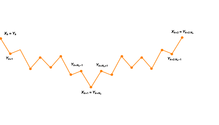
Figure 7: The points $X_{k}$, $X_{k+1}$, $X_{k+2}$, and $Y_{k}$, $\ldots$, $Y_{k+N_{b}}$, $\ldots$, $Y_{k+2\,N_{b}}$.

The values of $u_{m-1}$ in $X_{k}$, $X_{k+1}$, $X_{k+2}$ are thus supposed to be known.
The eigenvalue equation in $\Lambda_{m}$ leads to the following systems:

$$\left\{\begin{array}[]{ccccc}\left\{\Lambda_{m}-2\,h_{m-1}^{2}\right\}\,u_{m}\left(Y_{k+1}\right)&=&-h_{m-1}^{2}\,u_{m-1}\left(X_{k}\right)-h_{m-1}^{2}\,u_{m}\left(Y_{k+2}\right)&&\\ \left\{\Lambda_{m}-2\,h_{m-1}^{2}\,\right\}\,u_{m}\left(Y_{k+i}\right)&=&-h_{m-1}^{2}\,u_{m}\left(Y_{k+i-1}\right)-h_{m-1}^{2}\,u_{m}\left(Y_{k+i+1}\right)&,&1\leqslant i\leqslant N_{b}-3\\ \left\{\Lambda_{m}-2\,h_{m-1}^{2}\,\right\}\,u_{m}\left(Y_{k+N_{b}-1}\right)&=&-h_{m-1}^{2}\,u_{m-1}\left(X_{k+1}\right)-h_{m-1}^{2}\,u_{m}\left(Y_{k+N_{b}-2}\right)&&\end{array}\right.$$

and :

$$\left\{\begin{array}[]{ccccc}\left\{\Lambda_{m}-2\right\}\,u_{m}\left(Y_{k+N_{b}+1}\right)&=&-h_{m-1}^{2}\,u_{m-1}\left(X_{k+1}\right)-h_{m-1}^{2}\,u_{m}\left(Y_{k+N_{b}+2}\right)&&\\ \left\{\Lambda_{m}-2\,h_{m-1}^{2}\,\right\}\,u_{m}\left(Y_{k+N_{b}+i}\right)&=&-h_{m-1}^{2}\,u_{m}\left(Y_{k+N_{b}+i-1}\right)-h_{m-1}^{2}\,u_{m}\left(Y_{k+N_{b}+i+1}\right)&,&1\leqslant i\leqslant N_{b}-3\\ \left\{\Lambda_{m}-2\,h_{m-1}^{2}\,\right\}\,u_{m}\left(Y_{k+2\,N_{b}-1}\right)&=&-h_{m-1}^{2}\,u_{m-1}\left(X_{k+2}\right)-h_{m-1}^{2}\,u_{m}\left(Y_{k+2\,N_{b}-2}\right)&&\end{array}\right.$$

For the sake of simplicity, we set:

$$\Lambda_{m}=h_{m-1}^{2}\,\tilde{\Lambda}_{m}$$

The sequence $\left(u_{m}\left(Y_{k+i}\right)\right)_{0\leqslant i\leqslant 2\,N_{b}}$ satisfies a second order recurrence relation, the characteristic equation of which is:

$$r^{2}+\left\{\tilde{\Lambda}_{m}-2\right\}\,r+1=0$$

The discriminant is:

$$\delta_{m}=\left\{\tilde{\Lambda}_{m}-2\right\}^{2}-4=\omega_{m}^{2}\quad,\quad\omega_{m}\,\in\,\mathbb{C}$$

The roots $r_{1,m}$ and $r_{2,m}$ of the characteristic equation are the scalar given by:

$$r_{1,m}=\displaystyle\frac{2-\tilde{\Lambda}_{m}-\omega_{m}}{2}\quad,\quad r_{2,m}=\displaystyle\frac{2-\tilde{\Lambda}_{m}+\omega_{m}}{2}$$

One has then, for any natural integer $i$ of $\left\{0,\ldots,2\,N_{b}\right\}$ :

$$u_{m}\left(Y_{k+i}\right)=\alpha_{m}\,r_{1,m}^{i}+\beta_{m}\,r_{2,m}^{i}$$

where $\alpha_{m}$ and $\beta_{m}$ denote scalar constants.

The extension $u_{m}$ of $u_{m-1}$ to $V_{m}\setminus V_{0}$ has to be an eigenfunction of $\Delta_{m}$, for the eigenvalue $\Lambda_{m}$.
Since $u_{m-1}$ is an eigenfunction of $\Delta_{m-1}$, for the eigenvalue $\Lambda_{m-1}$, the sequence $\left(u_{m-1}\left(X_{k+i}\right)\right)_{0\leqslant i\leqslant N_{b}}$ must itself satisfy a second order linear recurrence relation which be the pendant, at order $m$, of the one satisfied by the sequence $\left(u_{m}\left(Y_{k+i}\right)\right)_{0\leqslant i\leqslant 2\,N_{b}}$, the characteristic equation of which is:

$$h_{m-2}^{2}\,\left\{\Lambda_{m-1}-2\right\}\,r=-1-r^{2}$$

and discriminant:

$$\delta_{m-1}=\left\{\Lambda_{m-1}-2\right\}^{2}-4=\omega_{m-1}^{2}\quad,\quad\omega_{m-1}\,\in\,\mathbb{C}$$

The roots $r_{1,m-1}$ and $r_{2,m-1}$ of this characteristic equation are the scalar given by:

$$r_{1,m-1}=\displaystyle\frac{2-\tilde{\Lambda}_{m-1}-\omega_{m-1}}{2}\quad,\quad r_{2,m-1}=\displaystyle\frac{2-\tilde{\Lambda}_{m-1}+\omega_{m-1}}{2}$$

For any integer $i$ of $\left\{0,\ldots,N_{b}\right\}$:

$$u_{m-1}\left(Y_{k+i}\right)=\alpha_{m-1}\,r_{1,m-1}^{i}+\beta_{m-1}\,r_{2,m-1}^{i}$$

where $\alpha_{m-1}$ and $\beta_{m-1}$ denote scalar constants.

From this point, the compatibility conditions, imposed by spectral decimation, have to be satisfied:

$$\left\{\begin{array}[]{ccc}u_{m}\left(Y_{k}\right)&=&u_{m-1}\left(X_{k}\right)\\ u_{m}\left(Y_{k+N_{b}}\right)&=&u_{m-1}\left(X_{k+1}\right)\\ u_{m}\left(Y_{k+2\,N_{b}}\right)&=&u_{m-1}\left(X_{k+2}\right)\\ \end{array}\right.$$

i.e.:

$$\left\{\begin{array}[]{ccccc}\alpha_{m}+\beta_{m}&=&\alpha_{m-1}+\beta_{m-1}&{\cal C}_{m}\\ \alpha_{m}\,r_{1,m}^{N_{b}}+\beta_{m}\,r_{2,m}^{N_{b}}&=&\alpha_{m-1}\,r_{1,m-1}+\beta_{m-1}\,r_{2,m-1}&{\cal C}_{1,m}\\ \alpha_{m}\,r_{1,m}^{2\,N_{b}}+\beta_{m}\,r_{2,m}^{2\,N_{b}}&=&\alpha_{m-1}\,r_{1,m-1}^{2}+\beta_{m-1}\,r_{2,m-1}^{2}&{\cal C}_{2,m}\\ \end{array}\right.$$

where, for any natural integer $m$, $\alpha_{m}$ and $\beta_{m}$ are scalar constants (real or complex).

Since the graph $\Gamma_{{\cal W}_{m-1}}$ is linked to the graph $\Gamma_{{\cal W}_{m}}$ by a similar process to the one that links $\Gamma_{{\cal W}_{1}}$ to $\Gamma_{{\cal W}_{0}}$, one can legitimately consider that the constants $\alpha_{m}$ and $\beta_{m}$ do not depend on the integer $m$:

$$\forall\,m\,\in\,{\mathbb{N}}^{\star}\,:\quad\alpha_{m}=\alpha\,\in\,{\mathbb{R}}\quad,\quad\beta_{m}=\beta\,\in\,{\mathbb{R}}$$

The above system writes:

$$\left\{\begin{array}[]{ccc}\alpha\,r_{1,m}^{N_{b}}+\beta\,r_{2,m}^{N_{b}}&=&\alpha\,r_{1,m-1}+\beta\,r_{2,m-1}\\ \alpha\,r_{1,m}^{2\,N_{b}}+\beta\,r_{2,m}^{2\,N_{b}}&=&\alpha\,r_{1,m-1}^{2}+\beta\,r_{2,m-1}^{2}\\ \end{array}\right.$$

One has then to consider the following configurations:

1. First case:
   

   For any natural integer $m$ :

   $$r_{1,m}\,\in\,{\mathbb{R}}\quad,\quad r_{2,m}\,\in\,{\mathbb{R}}$$

   and, more precisely:

   $$r_{1,m}<0\quad,\quad r_{2,m}<0$$

   since the function $\varphi$, which, to any real number $x\geqslant 4$, associates:

   $$\varphi(x)=\displaystyle\frac{2-x+\varepsilon\,\sqrt{\left\{x-2\right\}^{2}-4}}{2}\quad,\quad\varepsilon\,\in\,\left\{-1,1\right\}$$

   is strictly increasing on $]4,+\infty[$. Due to its continuity, is is a bijection of $]4,+\infty[$ on $\varphi\left(]4,+\infty[\right)=]-1,0[$.
   

   This configuration only occurs in the cases when the natural integer $N_{b}$ is an odd number. Let us introduce the function $\phi$, which, to any real number  $x\geqslant 2$, associates:

   $$\phi(x)=|\varphi(x)|=\displaystyle\frac{-2+x-\varepsilon\,\sqrt{\left\{x-2\right\}^{2}-4}}{2}$$

   where $\varepsilon\,\in\,\left\{-1,1\right\}$.

   The function $\phi$ is a bijection of $]4,+\infty[$ on $\phi\left(]4,+\infty[\right)=]0,1[$. We will denote by $\phi^{-1}$ its inverse bijection:

   $$\forall\,\,x\,\in\,]0,1[\,:\quad\phi^{-1}(x)=\displaystyle\frac{(y+1)^{2}}{y}$$

   .
   

   One has then:

   $$\varphi\left(\tilde{\Lambda}_{m-1}\right)=\displaystyle\frac{2-\tilde{\Lambda}_{m-1}+\varepsilon\,\omega_{m-1}}{2}\leqslant 0$$

   This yields:

   $$(-1)^{N_{b}}\,\left(\varphi\left(\tilde{\Lambda}_{m}\right)\right)^{N_{b}}=\varphi\left(\tilde{\Lambda}_{m-1}\right)\leqslant 0$$

   which leads to:

   $$\phi\left(\tilde{\Lambda}_{m}\right)=\left(\phi\left(\tilde{\Lambda}_{m-1}\right)\right)^{\frac{1}{N_{b}}}$$

   and:

   $$\tilde{\Lambda}_{m}=\phi^{-1}\left(\left(\phi\left(\tilde{\Lambda}_{m-1}\right)\right)^{\frac{1}{N_{b}}}\right)=\displaystyle\frac{\left\{\left(\phi\left(\tilde{\Lambda}_{m-1}\right)\right)^{\frac{1}{N_{b}}}+1\right\}^{2}}{\left(\phi\left(\tilde{\Lambda}_{m-1}\right)\right)^{\frac{1}{N_{b}}}}=\displaystyle\frac{\left\{\left(\displaystyle\frac{-2+\tilde{\Lambda}_{m-1}-\varepsilon\,\sqrt{\left\{\tilde{\Lambda}_{m-1}-2\right\}^{2}-4}}{2}\right)^{\frac{1}{N_{b}}}+1\right\}^{2}}{\left(\displaystyle\frac{-2+\tilde{\Lambda}_{m-1}-\varepsilon\,\sqrt{\left\{\tilde{\Lambda}_{m-1}-2\right\}^{2}-4}}{2}\right)^{\frac{1}{N_{b}}}}$$

2. Second case :
   

   For any natural integer $m$:

   $$r_{1,m}\,\in\,\mathbb{C}\setminus{\mathbb{R}}\quad r_{2,m}=\overline{r_{1,m}}\,\in\,\mathbb{C}\setminus{\mathbb{R}}$$

   Let us introduce:

   $$\rho_{m}=\left|r_{1,m}\right|\,\in\,{\mathbb{R}}^{+}\quad,\quad\theta_{m}=\text{arg}\,r_{1,m}\quad\text{if}\quad r_{1,m}\neq 0$$

   The above system writes:

   $$\left\{\begin{array}[]{ccc}\rho_{m}^{N_{b}}\,\left\{\gamma\,\cos\left(N_{b}\,\theta_{m}\right)+\delta\,\sin\left(N_{b}\,\theta_{m}\right)\right\}&=&\rho_{m-1}\,\left\{\gamma\,\cos\left(\theta_{m-1}\right)+\delta\,\sin\left(\theta_{m-1}\right)\right\}\\ \rho_{m}^{2\,N_{b}}\,\left\{\gamma\,\cos\left(2\,N_{b}\,\theta_{m}\right)+\delta\,\sin\left(2\,N_{b}\,\theta_{m}\right)\right\}&=&\rho_{m-1}^{2}\,\left\{\gamma\,\cos\left(2\,\theta_{m-1}\right)+\delta\,\sin\left(2\,\theta_{m-1}\right)\right\}\end{array}\right.$$

   where $\gamma$ and $\delta$ denote real constants.
   

   The system is satisfied if:

   $$\left\{\begin{array}[]{ccc}\rho_{m}^{N_{b}}&=&\rho_{m-1}\\ \theta_{m}&=&\displaystyle\frac{\theta_{m-1}}{N_{b}}\end{array}\right.$$

   and thus:

   $$\phi\left(\tilde{\Lambda}_{m}\right)=\left(\phi\left(\tilde{\Lambda}_{m-1}\right)\right)^{\frac{1}{N_{b}}}$$

   which leads to the same relation as in the previous case:

   $$\tilde{\Lambda}_{m}=\phi^{-1}\left(\left(\phi\left(\tilde{\Lambda}_{m-1}\right)\right)^{\frac{1}{N_{b}}}\right)=\displaystyle\frac{\left\{\left(\phi\left(\tilde{\Lambda}_{m-1}\right)\right)^{\frac{1}{N_{b}}}+1\right\}^{2}}{\left(\phi\left(\tilde{\Lambda}_{m-1}\right)\right)^{\frac{1}{N_{b}}}}=\displaystyle\frac{\left\{\left(\displaystyle\frac{-2+\tilde{\Lambda}_{m-1}-\varepsilon\,\sqrt{\left\{\tilde{\Lambda}_{m-1}-2\right\}^{2}-4}}{2}\right)^{\frac{1}{N_{b}}}+1\right\}^{2}}{\left(\displaystyle\frac{-2+\tilde{\Lambda}_{m-1}-\varepsilon\,\sqrt{\left\{\tilde{\Lambda}_{m-1}-2\right\}^{2}-4}}{2}\right)^{\frac{1}{N_{b}}}}$$

   where $\varepsilon\,\in\,\left\{-1,1\right\}$.

Thanks

The author would like to thank JPG for his patient re-reading, and his very pertinent suggestions and advices, and Robert Strichartz, who suggested the introduction of specific energies to fully take into account the very specific geometry of the problem. Special thanks to GL, thanks to whom I searched in the right direction. All this helped improving the original work.

References

- [BBR17] K. Barańsky, B. Bárány, and J. Romanowska. On the dimension of the graph of the classical Weierstrass function. Advances in Math., 265:791–800, 2017.
- [BD85] A. Beurling and J. Deny. Espaces de Dirichlet. i. le cas élémentaire. Annales scientifiques de l’É.N.S. 4 e série, 99(1):203–224, 1985.
- [BU37] A. S. Besicovitch and H. D. Ursell. Sets of fractional dimensions. Notices of the AMS, 12(1):18–25, 1937.
- [Fal85] K. Falconer. The Geometry of Fractal Sets. Cambridge University Press, 1985.
- [FOT94] M. Fukushima, Y. Oshima, and M. Takeda. Dirichlet forms and symmetric Markov processes. Walter de Gruyter & Co, 1994.
- [Har11] G. Hardy. Theorems connected with Maclaurin’s test for the convergence of series. The Proceedings of the Royal Society of London, s2-9(1):126–144, 1911.
- [Hun98] B. Hunt. The Hausdorff dimension of graphs of Weierstrass functions. Proc. Amer. Math. Soc., 12(1):791–800, 1998.
- [Kel17] G. Keller. A simpler proof for the dimension of the graph of the classical Weierstrass function. Ann. Inst. Poincaré, 53(1):169–181, 2017.
- [Kig89] J. Kigami. A harmonic calculus on the Sierpiński spaces. Japan J. Appl. Math., 8:259–290, 1989.
- [Kig93] J. Kigami. Harmonic calculus on p.c.f. self-similar sets. Trans. Amer. Math. Soc., 335:721–755, 1993.
- [Kig03] J. Kigami. Harmonic analysis for resistance forms. Journal of Functional Analysis, 204:399–444, 2003.
- [Man77a] B. B. Mandelbrot. The Fractal Geometry of Nature. San Francisco: W.H.Freeman & Co Ltd, 1977.
- [Man77b] B. B. Mandelbrot. Fractals: form, chance, and dimension. San Francisco: Freeman, 1977.
- [Mos02] U. Mosco. Energy functionals on certain fractal structures. Journal of Convex Analysis, 9(2):581–600, 2002.
- [RSS95] T. Zhang R. S. Strichartz, A. Taylor. Densities of self-similar measures on the line. Experimental Mathematics, 4(2):101–128, 1995.
- [Sab97] C. Sabot. Existence and uniqueness of diffusions on finitely ramified self-similar fractals. Annales scientifiques de l’É.N.S. 4 e série, 30(4):605–673, 1997.
- [Str99] R. S. Strichartz. Analysis on fractals. Notices of the AMS, 46(8):1199–1208, 1999.
- [Str06] R. S. Strichartz. Differential Equations on Fractals, A tutorial. Princeton University Press, 2006.
- [Tit77] E. C. Titschmarsh. The theory of functions, Second edition. Oxford University Press, 1977.
- [Wei72] K. Weierstrass. Über continuirliche Funktionen eines reellen Arguments, die für keinen Werth des letzteren einen bestimmten Differential quotienten besitzen, in Karl Weiertrass Mathematische Werke, Abhandlungen ii. Akademie der Wissenchaften am 18 Juli 1872, 2:71–74, 1872.