Equation of state, phonons, and lattice stability of ultra-fast warm dense matter

Abstract

Using the two-temperature model for ultrafast matter (UFM), we compare the equation of state, pair-distribution functions $g(r)$, and phonons using the neutral pseudoatom (NPA) model with results from density-functional theory (DFT) codes and molecular-dynamics (MD) simulations for Al, Li and Na. The NPA approach uses state-dependent first-principles pseudopotentials from an ‘all-electron’ DFT calculation with finite-$T$ XCF. It provides pair potentials, structure factors, the ‘bound’ and ‘free’ states, as well as a mean ionization $\bar{Z}$ unambiguously. These are not easily accessible via DFT+MD calculations which become prohibitive for $T/T_{F}$ exceeding $\sim 0.6$, where $T_{F}$ is the Fermi temperature. Hence, both DFT+MD and NPA methods can be compared up to $\sim 8$ eV, while higher $T$ can be addressed ${\it via}$ the NPA. The high-$T_{e}$ phonon calculations raise the question of UFM lattice stability and surface ablation in thin UFM samples. The ablation forces in a UFM slab are used to define an “ablation time” competing with phonon formation times in thin UFM samples. Excellent agreement for all properties is found between NPA and standard DFT codes, even for Li where a strongly non-local pseudopotential is used in DFT codes. The need to use pseudopotentials appropriate to the ionization state $\bar{Z}$ is emphasized. The effect of finite-$T$ exchange-correlation functional is illustrated via its effect on the pressure and the electron-density distribution at a nucleus.

I Introduction.

The equation of state (EOS) of common thermodynamic phases of matter is well understood. However, recent laser and shock-wave experiments have accessed novel ultrafast regimes of density and temperature which are of great theoretical and technological interest. The same physics appears during the injection of hot carriers in field-effect transistors and other nanostructures. Topics like inertial-confinement fusion bib2 , Coulomb explosions bib3 , space re-entry shielding, laser machining and ablation bib1 involve such regimes of warm dense matter (WDM). However, elementary approaches cannot be applied since the Coulomb coupling constant $\Gamma$, i.e., the ratio of the Coulomb energy to the kinetic energy, is larger than unity. The electrons may range from degenerate to Boltzmann-like, with $T/E_{F}\sim 1$ or larger, where $T$ is electron temperature in energy units, while $E_{F}$ is the Fermi energy. This causes a prohibitive increase in basis sets that span the many excited electronic states. WDMs pose a theoretical challenge for rapid accurate computations of properties like pressure, heat capacity, phonons and conductance needed even for equilibrium WDMs.

A class of WDMs known as ultra-fast matter (UFM) is produce when energy is deposited using an ultrafast pulsed laser on a metal surface Ping10 . The light couples strongly to the mobile electrons which equilibrate on femtosecond timescales, to a temperature $T_{e}$ (as high as many eV) while the much heavier ions and their strongly-bound core electrons remain essentially at their initial temperature $T_{i}$, i.e., usually the room temperature $T_{r}$. This two-temperature WDM ($2T$-WDM) phase with $T_{e}>T_{i}$ remains valid for timescales $t$ such that $\tau_{ee}<\tau_{ii}<t<\tau_{ei}$, where $\tau_{ee}$, $\tau_{ii}$ and $\tau_{ei}$ are the electron-electron, ion-ion and electron-ion temperature relaxation times, respectively. It has been shown for near-solid densities that $\tau_{ei}$ is of the order of picoseconds, and orders of magnitude longer than $\tau_{ee}$ and $\tau_{ii}$ Milchberg88 ; bib7 . For WDMs with $\theta=T/E_{F}$ small, similar relaxation times hold as seen in calculations for typical systems XRTS2016 . Experiments using femtosecond pump-probe techniques bib4 ; chen2013 provide data for quasi-equilibrium analogues of free energy and pressure, transport and relaxation processes. While many UFM samples do not conform to the $2T$ model (e.g., as in Medvadev et al. Medvadev2011 ), the $2T$ model provides a great simplification when it holds. Even for UFMs, theory and experiment are quite challenging as the system transits rapidly from a solid to a plasma depending on the pump energy. Hence a theoretical model that encompasses a wide range of material conditions is needed to describe the time evolving system as a series of static 2$T$ systems. The ‘quasi-equilibrium’ theory is applied to each static picture of the time evolving system.

In this work, we use the neutral pseudoatom (NPA) model, in the form given by Perrot and Dharma-wardana Dagens1 ; Dagens2 ; PerrotBe ; PDW95 ; MuriDW2008 ; MuriDW2013 , to study the $2T$-WDM regime of a few nominally simple metals, viz., aluminum, lithium and sodium. These are “simple” at ambient conditions since their valence electrons are “free-electron like” and energetically separated from the core electrons. The number $\bar{Z}$ of valence electrons per atom (mean ionization) for Al, Li, and Na is 3, 1, and 1, respectively. Furthermore, if the matter density is $\rho$, each ion can be assigned a spherical volume with the Wigner-Seitz (WS) radius $r_{ws}=(3/4\pi\rho)^{1/3}$, and it can be shown for Al, Li, Na that the bound-electron core has a radius $r_{c}$ such that it is well inside the WS sphere for the temperatures studied here (see Sec. IV.4). In such cases, the definition of $\bar{Z}=N-n_{b}$, where $n_{b}$ is the number of bound electrons in the core, is unambiguous, clear and is a physically measurable quantity, e.g., using X-ray Thomson scattering GlenzerRevMod . In the case of equilibrium WDM, the NPA-calculated $\bar{Z}$ for Al and Li remains 3 and 1 in the range $0<T_{e}<8$ eV whereas in the case of sodium, $\bar{Z}$ rises to 1.494 by T=8 eV and 1.786 by 10 eV. The case of Na provides us an example of a typical variation of $\bar{Z}$ very common in equilibrium WDM systems and handled without any ambiguity and with thermodynamic consistency by the NPA approach coupled with determinations of the ion-ion $g(r)$ using the NPA pair-potentials. However, in the case of UFM which is the scope of this work, $\bar{Z}$ is kept unchanged for all three elements through the $0<T_{e}<8$ eV temperature range.

The NPA model replaces the interacting many-nuclear and many-electron problem by an effective non-interacting single-nuclear and single-electron formulation where the many-body problem is reduced using finite-$T$ density functional theory (DFT) bib8 ; bib9 . The NPA charge densities are used to construct $2T$ pseudopotentials and effective ion-ion pair potentials. The method takes into account particle correlations at the pair-density level and beyond using density-functional methods via exchange-correlation functionals for electrons, and ion-correlation functionals for ions in a decoupled step which uses a classical integral equation or molecular dynamics. The NPA framework is well adapted to treating metallic systems ranging from solids to liquids or plasmas at very high or low compressions, and from $T$=0 to several keV. The importance and relevance of the NPA lies in its accuracy, flexibility, and computational rapidity compared to DFT coupled to molecular dynamics (MD) methods (DFT+MD). However, the NPA, as used here, is inapplicable when inner-shell electrons (e.g., $d$-electrons) play a role in the ion-ion interactions (e.g., as in transition metals). A simple metal becomes ‘complex’ when its electronic bound states extends beyond its WS radius $r_{ws}$. This is not a short-coming but a strength of the model which signals the need for multi-ion contributions into the theory in such ranges of temperature and pressure. In such regimes, discontinuities in $\bar{Z}$ where some are spurious may appear unless suitable electron-ion XC-correlation potentials are included in the theory Furutani90 . Furthermore transient molecule formation can be successfully handled carbonCDW16 within the NPA as it allows for binary ion-ion correlations.

We compare our $2T$-NPA predictions with those from solid-state DFT electronic-structure codes such as ABINIT bib19 and VASP VASP , which use MD to evolve the finite-$T$ ionic structures. These codes are primarily designed for $T_{i}=T_{e}=0$ situations, and solve the multi-nuclear Kohn-Sham equations in a plane-wave basis, using $T=0$ pseudopotentials to reduce the number of electrons needed in the simulations. The solid, liquid or plasma is treated as a periodic solid in a simulation box (“supercell”) containing $N$ nuclei, with $N$ being $\sim$100. A finite $T_{e}$ Fermi-Dirac distribution for electron occupation numbers is used, along with $T=0$ pseudopotentials and $T=0$ exchange-correlation functionals (XCF). The number of electronic bands required to access high $T_{e}$ increases rapidly with $T_{e}$ and becomes prohibitive for $T_{e}/E_{F}$ greater than $\sim 1$. This method generates energy bands for the periodic solid where as in reality there are no such band structure in liquids and plasmas. This artifact is overcome by generating electronic-structure calculations for many static ionic configurations via MD simulations and averaging over a large number of them.

DFT+MD provides only a “mean ionization” for the whole $N$-ion supercell; it cannot provide, e.g., the composition of an equilibrium mixture of specific charge states of ions in a C, H “plastic” at, say, 1 eV. Furthermore, VASP and ABINIT currently only implement the zero-$T$ XCF even though finite-$T$ parametrizations have been available for some time, e.g., the evaluation of finite-$T$ bubble diagrams bubble1 ; bubble2 , from the work of Iyetomi and Ichimaru Iye , Perrot and Dharma-wardana (PDW) PDWfxc and from Feynman-path methods by Brown et al Brown parametrized recently by Karasiev et al Karasiev . The present NPA calculations are done with the PDW finite-$T$ XCF which is in close agreement with the quantum simulations of Brown et al. cdw-cpp15 . In most cases finite-$T$ XC effects contribute only small corrections and DFT+MD provides valuable benchmarks for testing other methods.

The NPA method is summarized in section II where we emphasize its application to the $2T$ regime. Resulting $2T$ pair potentials ($2T$PP), quasi-equilibrium phonon dispersions and pair distribution functions (PDF) $g(r)$ are presented in Sec. III. The phonon calculations confirm the results and also validate the meV accuracy of the NPA method. The NPA $g(r)$ calculations for normal and compressed Li ($\sim$ up to a compression of 2) show that the local pseudopotential for Li is successful. Here we compare the ion-ion structure factor $S(k)$ with the simulations of Kietzmann et al. Having confirmed the accuracy of the pseudopotentials and pair potentials, the 2$T$-thermodynamic properties, such as the quasi-pressure, are also presented. These are compared with the values for systems in thermal equilibrium. Discussions about phonon formation times in $2T$ systems, the role of finite-$T$ XC-contributions in the $2T$-EOS calculation, and the choice of suitable pseudopotentials in ab initio finite-$T$ simulations are also presented.

II The neutral pseudoatom model.

II.1 General description of the model.

Several average-atom models and NPA models have been proposed, even in the early literature Ziman . Many of these are intuitive cell models and are not true DFT models. A rigorous DFT formulation of a NPA model at $T=0$ was first used for solids by Dagens Dagens1 ; Dagens2 . There the treatment of the ion distribution was developed in the traditional manner as providing a fixed external potential; Dagens showed that the NPA results at $T=0$ agree closely with the band-structure codes available at the time. A finite-$T$ version was given in several papers by Perrot PerrotBe and Dharma-wardana DWP1 ; PDW2 ; PDW3 . In Ref. DWP1 , the ion distribution $\rho(r)$ itself was treated within DFT using the property that the free energy $F[n,\rho]$ is a functional of both $n(r)$ and $\rho(r)$ simultaneously. A classical DFT equation for the ions and an ion-correlation functional, $F_{c}^{ii}(\rho)$, approximated as a sum of hypernetted-chain (HNC) diagrams plus bridge diagrams, was introduced, without invoking a Born-Oppenheimer approximation or treating the ions as providing a fixed external potential IlCiacco93 . Exchange-correlation functionals $F_{xc}^{ei}(\rho)$ for electron-ion interactions were also introduced although neglibible in common materials. This puts the NPA approach on a very rigorous DFT footing where approximations enter in modeling the ion-correlation functional, just as in the case of the electron DFT problem for the electronic XCF.

However, in the following we present the theory in terms of the more familiar superposition picture. We consider a system of ions located at sites $\mathbf{R}_{i}$ at temperature $T_{i}$ and average density $\rho$, interacting with a system of electrons at temperature $T_{e}$ and average density $n$. The multi-center problem is reduced to a simplified single-center problem where the total electron density $n(r)$ is regarded as the superposition of single-site densities such that $n(r)=\sum_{i}n_{i}(r-\mathbf{R}_{i})$. In contrast to ion-sphere (IS) models like those used in Purgatorio Purgatorio , or Piron and Blenski Blenski2011 , Starrett and Saumon Starrett2013 , the single-site free-electron density $n_{f}(r)$ extends over the whole of space, approximated by a correlation sphere DWP1 of radius $R_{c}$ which is of the order of 10 ionic Wigner-Seitz radii. All particle correlations are assumed to have died out when $r\to R_{c}$. This $R_{c}$ is similar to the linear dimension of the simulation box of a DFT+MD simulation which has to be as big as possible. However, in practice the charge distribution used in DFT+MD simulations spreads over a volume of about 100 ions. In contrast, the NPA correlation sphere with $R_{c}\simeq 10r_{ws}$ extends over $\{R_{c}/r_{ws}\}^{3}$, i.e., the volume covered by $\sim$1000 ions. The calculation of course uses only one nucleus, but its charge density overlaps the space of some 1000 atoms, and this is crucial to getting the right pair-potentials with long-range Friedel oscillations, and to satisfy the Friedel sum rule DWP1 . The IS-models cannot satisfy the Friedel sum rule. At higher temperatures where particle correlations are weak, $r_{c}$ may be reduced to, e.g., $5r_{ws}$, but the results are independent of $R_{c}$, and $R_{c}$ is not an optimization parameter.

The ion distribution $\rho(r)=\rho g_{ii}(r)$ contains the full ion-ion PDF, $g(r)$, when seen from any site taken as the origin. It is found that in most cases it is sufficient, as far as the bound-electron structure is concerned, to approximate $g(r)$ by a spherical cavity $c(r)$ of radius $r_{ws}$ and total charge $\bar{Z}$ centered on the ion, followed by a uniform positive density $\rho$ for $r>r_{ws}$. As mentioned below, unlike in IS-models, its effect will be subtracted out (as a “cavity correction”) to obtain the response of a uniform electron gas to the nucleus. Thus have:

$$c(r)=n[H(0)-H(r-r_{ws})],$$ (1)

where $H(r)$ is the Heaviside step function. Initially $\bar{Z}$ is unknown but its value is obtained self-consistently from the iterative Kohn-Sham procedure. The single-site electron density is written as $n_{i}=\Delta n_{i}+m_{i}$ where $m_{i}$ is the cavity correction and $\Delta n_{i}$ is the electron pile-up obtained by the DFT calculation for the electrons in the external potential $V_{\text{ext}}$ given by

$$V_{\text{ext}}(r)=-\frac{Z}{r}+\frac{1}{|\mathbf{r}-\mathbf{r}^{\prime}|}\star c(\mathbf{r}^{\prime})$$ (2)

where the symbol $\star$ means integration over all space. Here $Z=Z_{n}$ is the nuclear charge. The positive background with the WS-cavity, the nucleus at its center and the free-electron charge density filling the whole correlation sphere constitute the neutral pseudoatom PDW2 ; PDW3 . The WDM system is made up of superpositions of such neutral-pseudo atoms correlated to give the ion-ion $g(r)$, with the cavity contributions subtracted out.

For simple metallic systems, this cavity model that defines the extent of the bound states is sufficient to produce physically accurate results and is mathematically convenient, as shown in the papers by Dagens or those of Perrot and Dharma-wardana cited above. Thus, to compute the cavity correction $m(r)$, we assume that the electrons respond linearly to the cavity $c(r)$, viz., in Fourier space,

$$m(q)=-V(q)c(q)\chi_{ee}(q,n,T_{e}).$$ (3)

Here, $V(q)=4\pi/q^{2}$ is the Coulomb potential and $\chi_{ee}$ is the interacting-electron response function at the electron density $n$ and temperature $T_{e}$. To go beyond the random phase approximation (RPA), we use the following finite-$T$ response function:

$$\chi_{ee}(q,n,T_{e})=\frac{\chi_{0}(q,n,T_{e})}{1-V(q)[1-G(q)]\chi_{0}(q,n,T_{e})},$$ (4)

with $\chi_{0}$ the finite-$T$ Lindhard function and $G(q)=G(q,T_{e})$ a local-field correction (LFC) defined as:

$$G(q)=\left(1-\frac{\gamma_{0}}{\gamma}\right)\left(\frac{q}{k_{\text{TF}}},\right)^{2}.$$ (5)

In the above, the Thomas-Fermi wave vector $k_{\text{TF}}=\sqrt{6\pi n/E_{F}}$, is defined by the Fermi energy of the system $E_{F}=1/(\alpha r_{s})$ where $r_{s}$ is the electron WS radius and $\alpha=(4/9\pi)^{1/3}$. The finite-$T$ interacting electron compressibility $1/\gamma=n^{2}\partial^{2}[nf(r_{s},T_{e})]/\partial n^{2}$ is determined from the homogenous electron gas free energy per electron $f(r_{s},T_{e})$, as given in Eq.13, which include a finite-$T$ XC contribution $f_{xc}$. The non-interacting electron compressibility $\gamma_{0}$ is obtained by setting $f_{xc}=0$.

The simplicity of the NPA model rests on decomposing the total charge distribution into a superposition of single-center distributions. If the ion-ion structure factor $S_{ii}(q)$ is known, any total electron charge distribution $n_{t}(q)$ can always be written as a convolution of the $S_{ii}(q)$ with some effective single-center charge distribution $n(q)$, even for transition metals or systems with resonant levels; but partitioning the electron contributions from states that extend beyond their WS cells without correctly including the physical interactions is not sufficient. Furthermore, a ‘simple metal’ at one temperature may behave as a ‘transition-metal’ at another temperature when a shell of electrons begins to transit to the continuum, and vice versa. If the system is of such low density that $r_{ws}$ is larger than the bond length of a possible dimer (e.g., Li₂), then the dimer itself will be contained within the WS sphere, and in such cases the NPA model fails; a more elaborate “neutral-pseudomolecule” approach or the use of suitable electron-ion XC-potentials $F_{xc}^{ei}(n,\rho)$ is then needed. We do not examine such non-simple WDMs in this study. Similarly, at high densities, WDM-Li shows complex phases containing persistent Li₄ clusters bonev2008 , and the simple NPA model needs modifications. In the present case, a single-center decomposition is physically transparent if the bound electron core is unambiguously confined within the WS sphere of the ion. We discuss in the results section (sec. IV.4) the variation of the $\bar{Z}$ of Na which changes from unity at low $T$ to 1.49 by $T=8$ eV. The occupation number in the 2$p$ level begins to decrease, while its radius slightly decreases, and hence there is no ambiguity in estimating $\bar{Z}=Z-n_{b}$ where $n_{b}$ are all the bound electrons compactly contained well inside the WS-sphere. That is, the electron density pileup $\Delta n_{i}$ can be clearly divided into bound and free parts such that $\Delta n_{i}=n_{b}+n_{f}$. Once this division is achieved the interaction of an electron with the nucleus plus its core can in most cases be replaced by a pseudopotential $U_{ei}$ which is a weak scatterer because it is constructed using linear response; this is given by:

$$U_{ei}(q)=n_{f}(q)/\chi_{ee}(q,r_{s},T_{e}),$$ (6)

where $\chi_{ee}$ is provided by Eq. 4.

Even though linear response is used, the resulting pseudopotential includes non-linear effects since $n_{f}(q)$ is the fully non-linear free-electron density obtained from DFT. Only a range of $q$ between zero to slightly above $2k_{F}$ (depending on $T_{e}$) needs to be included as the large-$q$ behavior (short-range in $r$, i.e., inside the core) is not relevant. The resulting pseudopotential is valid only if it satisfies the relation $U_{ei}/(-\bar{Z}V(q))\leq 1$. Unlike the pseudopotentials used in VASP, ABINIT and similar DFT codes, this linear-response pseudopotential does not require solving a Schrödinger equation. It is a state-dependent local pseudopotential that can be fitted to, say a Heine-Abarankov form for convenience (see Shaw and Harrison HA ). This has a constant core potential $V_{\text{HA}}=D$ for $r<r_{c}$ and it is Coulomb-like, $V_{\text{HA}}=-\bar{Z}/r$ for $r>r_{c}$. However, such a fitting is not needed except to conveniently report the pseudopotential and to quantify the core radius associated with the potential. In our NPA calculations we use the numerical form of $U_{ei}(q)$ directly.

The pseudopotential calculated at $T_{i}$ can be used to form a $2T$ ion-ion pair potential ($2T$PP) with ions at $T_{i}$ and electrons at $T_{e}$, since it is a sum of the direct Coulomb interaction and the indirect interaction via the displaced-electron charge, viz.

$$U_{ii}(q,T_{i},T_{e})=-\bar{Z}^{2}(T_{i})V(q)+|U_{ei}(q)|^{2}\chi_{ee}(q,T_{e}).$$ (7)

This procedure is valid because $\bar{Z}$ remains unchanged in UFM since the bound core of electrons remains at the initial ion temperature for times $t<\tau_{ei}$. If $T_{e}$ is large enough to change $\bar{Z}$, be it for UFM or equilibrium systems, then the pseudopotential has to be re-calculated using an NPA calculation at the needed temperature.

At low $T_{e}$, the Friedel oscillations in the electron density resulting from the sharp discontinuity at $k=2k_{F}$ in $\chi_{ee}(q)$ produce oscillations in the pair potential $U_{ii}(r)$. These lead to multiple minima in the ion-ion energy which contribute to the maxima in $g(r)$. Such physically important features are not found in “Slater-sum” approaches Slatersum to finite-$T$ potentials, in ‘Yukawa-screening’ models YukawaScr ; XRTS2016 , or in Gordon-Kim models Gordon-Kim72 . Furthermore, the charge densities restricted to the WS-sphere used in IS-models cannot capture such long-range effects. Our NPA pair potential can be used to study phonons in the system or to generate the ion-ion $g_{ii}(r)$ and corresponding structure factor $S_{ii}(k)$ when necessary. The ion subsystem in a UFM is clamped at $T_{i}\sim 300$K when Al, Li, and Na are crystalline metals. Hence the ion-ion pair distribution function is simply given by the relation

$$g_{ii}(\mathbf{r})=\frac{1}{4\pi\rho}\sum_{\{i\}}\delta(\mathbf{r}-\mathbf{R}_{i}).$$ (8)

The summation is over the crystal lattice, permitting a simple computation of the ion contribution to the quasi free energy and pressure from the $2T$ pair potential.

II.2 The NPA quasi thermodynamic relations.

The total free energy $F$ of the $2T$ system given by the NPA is

$$F=F_{\text{emb}}+F_{\text{cav}}+F_{\text{heg}}+F_{\text{ion}},$$ (9)

where $F_{\text{heg}}$, $F_{\text{emb}}$, $F_{\text{cav}}$, and $F_{\text{ion}}$ are respectively the free energy contribution of the interacting homogeneous electron gas (HEG), the embedding free-energy of the NPA into the electron gas, the correction from the cavity, and the ion-ion free energy. The only parameters of this model are the nuclear charge $Z$, electron temperature $T_{e}$ and the HEG density $n$ such that the average ion density $\rho=n/\bar{Z}$, itself determined by the ion temperature $T_{i}$. We discuss these four terms below, using Hartrees with $\hbar=m_{e}=|e|=1$.

(i) The embedding energy $F_{\text{emb}}$ is the difference between the free energy of the electron gas containing the central ion and the unperturbed HEG; thus

$$F_{\text{emb}}=T[n+\Delta n(r)]-T[n]-\int\frac{\bar{Z}}{|\mathbf{r}|}\cdot[\Delta n(\mathbf{r})+c(\mathbf{r}))]d\mathbf{r}$$

$$+\frac{1}{2}\int\frac{[\Delta n(\mathbf{r})+c(\mathbf{r})]}{|\mathbf{r}-\mathbf{r}^{\prime}|}\cdot[\Delta n(\mathbf{r}^{\prime})+c(\mathbf{r}^{\prime})]d\mathbf{r}d\mathbf{r}^{\prime},$$ (10)

with $T[n]$ is the electron kinetic energy.

(ii) The cavity correction $F_{\text{cav}}$ is computed from the total screened Coulomb potential $V(r)$ resulting from the total electron displacement $\Delta n(r)$:

$$V^{*}_{i}(\mathbf{r})=\int\frac{[c(\mathbf{r}^{\prime})+\Delta n(\mathbf{r}^{\prime})-\bar{Z}\delta(\mathbf{r}^{\prime}-R_{i})]}{|\mathbf{r}-\mathbf{r}^{\prime}|}d\mathbf{r}^{\prime}.$$ (11)

Since each cavity involves a charge deficit $\eta(r)=n-c(r)$, the cavity correction is

$$F_{\text{cav}}= -\frac{1}{2}\int\frac{\eta(\mathbf{r})\cdot[c(\mathbf{r}^{\prime})-m(\mathbf{r}^{\prime})]}{|\mathbf{r}-\mathbf{r}^{\prime}|}d\mathbf{r}d\mathbf{r}^{\prime}$$ (12)

$$+\int\eta(\mathbf{r})\cdot V^{*}(\mathbf{r})d\mathbf{r}.$$

(iii) The free energy of the HEG $F_{\text{heg}}$ is written as

$$F_{\text{heg}}=\bar{Z}f(n,T_{e})=\bar{Z}[f_{0}(n,T_{e})+f_{xc}(n,T_{e})],$$ (13)

where $f_{0}$ and $f_{xc}$ are respectively the non-interacting and exchange-correlation free energies per electron at the density $n$ and temperature $T_{e}$. To compute $f_{0}$, we use the thermodynamic relation $f_{0}=\Omega_{0}/nV+\mu_{0}$, where $\Omega_{0}$ and $\mu_{0}$ are the non-interacting grand potential and the chemical potential, respectively.

We emphasize that the NPA-Correlation-sphere model uses the non-interacting $\mu_{0}$ associated with the mean electron density $n$ as required by DFT theory. In IS models the known matter density defines the Wigner-Seitz cell, and the free electrons are confined in it, and the corresponding $\mu$ is determined by an integration within the WS-sphere (e.g., see Eq. 1 of Faussurier Faussurier2014 ), leading to a value of $\mu\neq\mu_{0}$. In contrast, the mean electron density $n$, the nuclear charge $Z_{n}$ and the temperature $T$ are the only inputs to the NPA code. The computation outputs the corresponding mean ion density $\rho$ and $\bar{Z}=n/\rho$. A series of calculations are done in a range of $n$ and the specific $n$ which gives the physical ion density, viz., $\rho$ is selected. For a given electron density $n$ and temperature $T_{e}$, the non-interacting chemical potential $\mu_{0}$ is obtained by satisfying the relation

$$n=(\sqrt{2}/\pi^{2})T_{e}^{3/2}\ I_{1/2}(\mu_{0}/T_{e}),$$ (14)

while, using this $\mu_{0}$, the non-interacting part of the grand potential is given by

$$\Omega_{0}/V=(2\sqrt{2}/3\pi^{2})T_{e}^{5/2}\ I_{3/2}(\mu_{0}/T_{e}),$$ (15)

with $I_{\nu}(z)$ the Fermi-Dirac integral of order $\nu$. Note that only the non-interacting chemical potential, viz., $\mu_{0}$ appears in the DFT-level occupations of the NPA model since DFT theory maps the interacting electrons to a system of non-interacting electrons at the interacting density (see also Ref. DWP1 ).

The XC contribution $f_{xc}$ is computed directly from the PDW parametrization at the given $r_{s}$ and $T_{e}$. The total free energy per electron of the interacting HEG is the sum of $f_{0}$ and $f_{xc}$.

(iv) The ion-ion interaction energy is given explicitly by the pairwise summation over the pair potential $U_{ii}$ as defined at Eq.(7):

$$F_{\text{ion}}=\frac{1}{V}\frac{1}{2}\sum_{\{i\neq j\}}U_{ii}(|\mathbf{R}_{i}-\mathbf{R}_{j}|),$$ (16)

where the sum is over the positions of the ions in their initial crystal configuration. This is the only term in $F$ that depends explicitly on the ion structure.

Both the cavity correction and the embedding energy involve the ion with its bound core of electrons held at the temperature $T_{i}$, while the electrons are at $T_{e}$. The numerical results are insensitive to using a simple NPA calculation with even the core at $T_{e}$, if the the bound-state occupancies (and thus $\bar{Z}$) remain virtually unchanged.

The quasi-equilibrium pressure of the system is obtained by the appropriate density derivative of the ion-structure independent free energy terms while the structure-dependent ion-ion contribution is given by the viral equation

$$P =n^{2}\frac{\partial}{\partial n}(F_{\text{heg}}+F_{\text{emb}}+F_{\text{cav}})$$ (17)

$$-\int g_{ii}(\mathbf{r})\left(\frac{3}{r}\frac{\partial}{\partial r}-n^{2}\frac{\partial}{\partial n}\right)U_{ii}(\mathbf{r})d\mathbf{r}.$$

The explicit electron-density dependence of the ion-ion pair potential is taken into account in computing the pressure Hansen . Analytical results can be obtained for the terms

$$P_{\text{emb}}=-\int\eta(\mathbf{r})\cdot V^{*}(\mathbf{r})d\mathbf{r}$$ (18)

$$P_{\text{cav}}=-\bar{Z}V^{*}(r_{ws})$$ (19)

whereas other derivatives have to be done numerically.

III Results.

We used the NPA model to determine the properties of $2T$-WDM as produced by femtosecond laser pulses interacting with three common metals in their usual solid state, viz., aluminum, lithium and sodium, with electron densities such that $r_{s}$ is 2.07, 3.25, and 3.93 a.u., corresponding to $\bar{Z}$ = 3, 1 and 1, respectively. Note that the $\bar{Z}$ for Na deviates from unity for $T>3$ eV. The ion density is kept constant in the calculations for isochoric sodium. We present the $2T$ ion-ion pair-potentials, non-equilibrium phonon dispersion curves and pressures for varying $T_{e}$, while the ions remain cold at $T_{i}=$0.026 eV (300K).

III.1 Ion-ion pair potentials.

The first step within our UFM model is to compute the equilibrium (at room temperature, $T_{e}=T_{i}=0.026$ eV) free-electron density $n_{f}(q)$ from the NPA calculation. The pseudopotential $U_{ei}(q)$ at $T_{e}=T_{i}$ can then be obtained using Eq. 6. This pseudopotential is an atomic property that depends on $\bar{Z}$ and on the core radius given the ionic $r_{ws}$, which is then used to construct ion-ion pair potentials $U_{ii}(q,T_{e})$ at any $T_{e}$ via Eq. (7). For this the electron response at $T_{e}\neq T_{i}$ is used. This method is simpler and numerically almost indistinguishable from calculating the pseduopotential from a full 2$T$-NPA procedure where the core electrons are held frozen at $T_{i}$ and $n_{f}(q,T_{e})$ is calculated from the Kohn-Sham equation, with $\bar{Z}$ remaining unchanged. The agreement between the two different ways of calculating the 2$T$ potentials provides a strong check on our calculations. Furthermore, while pair potentials cannot be easily extracted from ab initio calculations, the NPA model provide this physically important quantity.

Examples of NPA ion-ion pair potentials at different temperatures are presented in Fig. 1. At equilibrium or sufficiently low $T_{e}$, all three pair potentials display Friedel oscillations as discussed in section II. Hence it requires many neighbor shells to compute the total pairwise ion-ion interaction energy with sufficient precision. For Li and Na, we used 8 shells whereas 30 shells were necessary for the Al-Al interaction. As $T_{e}$ increases, the sharp Fermi surface breaks down, the discontinuity in $f(k)$ at $k=k_{F}$ broadens, and oscillations disappear, yielding purely repulsive Yukawa-screened potentials YukawaScr .

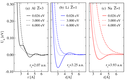
Figure 1: (Color online) Two-temperature ion-ion pair potentials for electrons at three different temperatures and ions at $T_{i}=0.026$ eV (300 K), for (a) Al, (b) Li, and (c) Na.

III.2 $2T$ quasi-equilibrium phonon spectra.

As the electrons get heated, the screening weakens and inter-ionic forces become stronger; hence there is an interest in computing the phonon spectra although in many cases the phonon oscillation times may be comparable to the lifetime of the UFM system. Once the 2TPP is constructed for the desired $T_{e}$, the phonon spectra are easily calculated by the diagonalization of the dynamical matrix AshcroftBk

$$\mathbf{D}(\mathbf{k})=\sum_{i}\mathbf{D}(\mathbf{R}_{i})e^{-i\mathbf{k}\cdot\mathbf{R}_{i}}\quad$$ (20)

where the elements of the harmonic matrix $\mathbf{D}(\mathbf{R})$ are given by

$$D_{\mu\nu}(\mathbf{R})=\frac{1}{2}\sum_{j}\frac{\partial^{2}U_{ii}(\mathbf{R}_{j})}{\partial u_{\mu}(\mathbf{R})\partial u_{\nu}(\mathbf{0})}$$ (21)

with $\mathbf{R}_{j}$ the position of the $j$th atom and $U_{ii}$ the pair-potential of Eq.7. From the $s$ eigenvalues $\lambda_{s}(\mathbf{k})$ of $\mathbf{D}(\mathbf{k})$, the phonon frequencies are given by $\omega_{s}(\mathbf{k})=\sqrt{\lambda_{s}(\mathbf{k})/M}$ with $M$ the mass of the ion. The resulting phonons are compared with the results from ABINIT-DFT simulations employing density-functional perturbation theory bib201 ; bib202 (DFPT), which determines the second derivative of the energy using the first-order perturbation wavefunctions. We used the common crystal structure for each metal, i.e., face-centered cubic (FCC) for Al and body-centered cubic (BCC) for Li and Na, with their room temperature lattice parameters $a=4.05\ \text{\AA},3.49\ \text{\AA}$, and $4.23\ \text{\AA}$, respectively.

Quasi-equilibrium phonon dispersion relations at $T_{e}=6$ eV using the two methods are presented in Fig. 2 with the NPA equilibrium phonons as reference to illustrate important modifications in the spectra. In addition, NPA quasi-equilibrium phonon spectrum at $T_{e}=12$ eV are also presented by which temperature DFPT becomes prohibitive. The excellent accord between the NPA and experimental equilibrium phonon spectra at low temperatures has already been demonstrated and shows the meV accuracy of the NPA calculations even at low temperatures CPP-Harb . This regime can be hard to model as noted by Blenski et al. Blenski2013 when, for example, working on Al at normal density and at low $T$ within another model.

For the three systems in this study, the two methods (NPA and DFPT) predict very similar $2T$ phonon spectra, thus reconfirming the $2T$ NPA calculations and corroborating the DFPT calculations at finite $T$. This is important as there are as yet no experimental observations of UFM phonon spectra. In the case of Al, we observe a large increase in frequencies, as high as $32\%$ for longitudinal (L) modes, which supports the “phonon hardening” theory. However, we notice that transverse (T) branches in the $\Gamma-L$ region are barely affected by the electron heating, as was also noted by Recoules Recoules . In the case of Li and Na, we find that the spectral modifications are more complex than the ‘homogeneous’ increase found for Al; here, an important increase in the L-branch in the middle of the $\Gamma-H$ region takes place, whereas there is no change at the symmetry point $H$. No modifications to T-branches are noticed in this region. In the region $H-\Gamma$, the L-branch frequencies increase in the middle of the region $H-P$ but remain unchanged at the symmetry point $H$. For the T-branch, an increase is noticeable at the maximum in the region $P-\Gamma$ whereas no change affects the minimum in the region $H-P$. In the region $\Gamma-N$ and for the L-branch, we observe the overall largest increase of $29\%$ and $37\%$ for Li and Na, respectively, whereas frequencies of T-modes are only slightly modified.

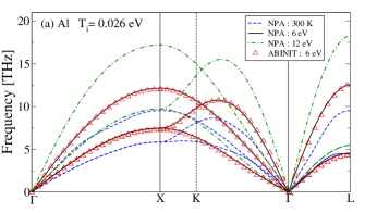
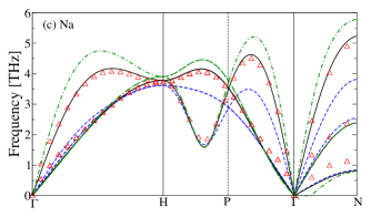
Figure 2: (Color online) Quasi-equilibrium phonon spectra at $T_{e}=6$ eV obtained with NPA and with ABINIT for (a) Al, (b) Li, and (c) Na. The NPA equilibrium phonon spectra at 300 K are shown to illustrate the effect of increasing $T_{e}$ (dashed lines).

III.3 $2T$-quasi-equilibrium equation of state.

A system in its initial equilibrium configuration ($T_{i}=T_{e}=T_{r}$) rapidly reaches a new UFM state with $T_{i}$ remaining near $T_{r}$ while $T_{e}$ increases. However, since the ion motion within the time of arrival of the probe pulse is negligible, the pressure builds up essentially isochorically due to electron heating.

In Fig 3, we compare the pressure calculated with the NPA model with ABINIT and VASP simulations. In the latter, we used an energy cut-off of 1630 eV for the plane-wave basis, with 60 energy bands to capture finite-$T$ effects. In ABINIT simulations, we used norm-conserving (NC) pseudopotentials with the $T=0$ Perdew-Burke-Ernzerhof (PBE) XCF within the generalized gradient approximation (GGA). In VASP, we employed projected-augmented-wave (PAW) pseudopotentials with the PBE XCF for Li and Na, and the Perdew-Wang (PW) $T=0$ XCF for Al. With both codes, pseudopotentials were chosen specifically to simulate $\bar{Z}$=3 valence electrons for Al, and $\bar{Z}$=1 for Li and Na as the core electrons remain bound, and at the ion temperature. This is an important aspect discussed in subsection IV.4.

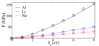
Figure 3: (Color online) Quasi-equilibrium pressures obtained with the NPA (lines), ABINIT (circles), and VASP (triangles) for Al, Li, and Na.

We find that, for all three metals, calculations using NPA, ABINIT and VASP predict nearly identical pressures with small deviations only at high $T_{e}$. At $T_{e}=8$ eV, the maximum difference between all model is 9 GPa, 4 GPa and 3 GPa for Al, Li, and Na, respectively. Thus, the results from the extension of the NPA model to the $2T$ regime confirms the usability of the solid-state codes at least up to 6 eV on the one hand, and on the the other hand the validity of the NPA approach. However, since NPA uses a finite-$T$ XC-functional whereas ab initio simulations do not, the effect of such finite-$T$ corrections will be reviewed in section IV.

The computational efficiency and accuracy of the NPA approach make it a valuable tool for studying WDM and other complex systems where iterative computations of materials properties like $2T$ EOS, $2T$ specific heat, transport properties, opacities, energy-relaxation times, etc., are needed as the system evolves with time, since mean ionization, pair-potentials and structure factors are readily obtained. A few minutes on a desktop computer is sufficient in NPA calculations to generate accurate results which require long and intensive computations with DFT+MD.

IV Discussion.

IV.1 Crystal-lattice stability.

As electrons absorb the laser energy (within fs timescales) and heat up to $T_{e}$, the internal pressure of the system becomes very high as discussed in section III-C. In metals, the thermal expansion is also caused by the free-electron pressure. We studied the crystal stability of the solids as a function of lattice expansion; the results are presented in Fig. 4.

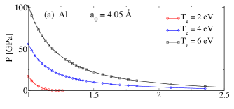
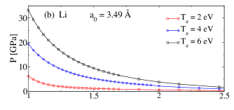
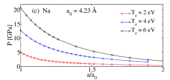
Figure 4: (Color online) Total pressure of the solids as a function of the lattice parameter of the crystal relative to the room-temperature value $a_{0}$ for (a) Al, (b) Li, and (c) Na.

For Al at $T_{e}=2$ eV, we find that a moderate expansion $a/a_{0}=1.24$ is sufficient to reduce the pressure back to zero, indicating that the crystal may appear stable if the timescale needed for such lattice motion is available before the UFM breaks down. However, in all other cases, the pressure goes to zero only asymptotically with increasing lattice parameter, suggesting that such UFM crystals are unstable. Such thermal expansions or spontaneous fluctuations lead to the ‘explosive’ breakdown of the solid on ps timescales. However, since UFM conditions are reached in fs timescales, the ions remain essentially in their initial positions and (as already noted) no net linear forces act upon them due to crystal symmetry. They remain trapped in a stronger harmonic potential leading to hardening of most of the phonon branches. The physical reason for the hardening at increased $T_{e}$ is the decreased screening of ion-ion interactions by the hotter electron gas.

IV.2 “Phonons” and surface ablation.

The UFM system is under very large pressure and the ion-ion $2T$PP is purely repulsive unless $T_{e}$ is small (cf. Fig. 1). The discussion in terms of phonons may become inapplicable at higher $T_{e}$ due to non-zero ablation forces acting on ions in typical UFM samples (0.1-1$\mu m$ thick). An ideal periodic lattice implies that the linear derivative of the total potential is zero because the crystal is isochorically constrained by the external pressure. The phonons of UFM “exist” only within this artifice. Small thermal ‘Debye-Waller’ type ionic displacements $u$ (with a mean value $\langle u\rangle=0.2\text{\AA}$ at 300K for Al, retained in the UFM) do not render the periodic UFM unstable, and slightly split the degeneracy of transverse branches.

However, pump-probe experiments use very thin metal films. Crystal symmetry is broken and large uncompensated forces act at the surface of the films; as a result, the surface layer and successive layers ablate. We calculated the ablation force $F_{\text{abl}}^{\text{VASP}}$ on an FCC-(100) Al surface and the two inner layers using the VASP code with the Al surface reconstructed as happens for the cold surface at 0K. Five layers of Al and 5 layers of vacuum were used for evaluating the Hellman-Feynman forces on the surface atoms. The NPA method is beyond its regime of validity since the charge density at a surface is not uniform. However, the NPA pressure is the force per unit area at the bounding (100) surface, with one ion per unit area. This is used as the NPA estimate of the ablation force $F_{\text{abl}}^{\text{NPA}}$. The forces on the inner neighbor and next-neighbor layers calculated from VASP at $T_{e}=$6 eV were 3% and 0.02% respectively of the force on the surface layer. The surface force $F_{\text{abl}}$ determines an approximate “ablation time” $\tau_{\text{abl}}$, the time needed for the surface plane to move by an inter-plane distance ($a/2$ in the case of Al). This $\tau_{\text{abl}}$ estimate makes some assumptions, e.g., $F_{\text{abl}}$ to be constant over $a/2$, with no movement of inner layers. To verify if phonons can form within such timescales, we compare $\tau_{\text{abl}}$ with the shortest time for an ion oscillation $\tau_{\omega}$ at the highest phonon frequency for the [100] direction; the results are presented in Table 1.

Table 1: The “ablation force” $F_{\text{abl}}$ and the “ablation time” $\tau_{\text{abl}}$ for the (100) surface of an Al slab from VASP and NPA at three different electron temperatures $T_{e}$ and lattice temperature $T_{i}=0.026$ eV. The fastest [100] phonon oscillation time $\tau_{\omega}$ is also given for each $T_{e}$.

$T_{e}$	$F_{\text{abl}}^{\text{NPA}}$	$F_{\text{abl}}^{\text{VASP}}$	$\tau_{\text{abl}}^{\text{NPA}}$	$\tau_{\text{abl}}^{\text{VASP}}$	$\tau_{\omega}$
eV	eV/Å	eV/Å	fs	fs	fs
2.00	0.91	0.90	111	111	105
4.00	2.75	2.70	63.9	64.2	92.6
6.00	5.03	4.70	47.1	48.6	80.6

As $T_{e}$ increases, phonons “harden” and $F_{\text{abl}}$ increases. In order to observe the “hardening” of phonons on any measurement, a probe time $\tau_{\text{pr}}$ such that $\tau_{\omega}<\tau_{\text{pr}}<\tau_{\text{abl}}$ is required. However, for sufficiently high $T_{e}$ (e.g., above $\sim 2$ eV for Al), the $F_{\text{abl}}$ are strong enough to make $\tau_{\text{abl}}<\tau_{\omega}$. Hence the ion oscillations have no time to build up and it is probably impossible to satisfy the time constraint enabling the observation of hardened phonons. The phonon concept itself becomes misleading for thin UFM films. Interpreting experiments when $\tau_{\text{pr}}>\tau_{\text{abl}}$ may require explicit inclusion of surface ablation corrections in the theory used for analyzing optical data (e.g., in the Helmholtz equations).

IV.3 Finite-$T$ exchange and correlation.

In the NPA model, we used the finite-$T$ XCF of PDW and assessed the importance of such corrections in the temperature regime studied here. The valence density, or “free”-electron density $n_{f}(r)$ of the solid at $T_{e}>T_{i}$ is the key quantity for the NPA model. In Fig. 5, we present the $n_{f}(r)$ obtained using the PDW finite-$T$ XCF with that obtained from the zero-$T$ XCF. Even though the correction is small, it may be of importance in some circumstances, e.g., x-ray Thomson scattering spectra, and hence there is no reason to neglect it. The difference between the $T=0$ XCF and the finite-$T$ XCF increases with $\theta=T/E_{F}$ at first, and it rapidly and asymptotically goes to zero as $\theta>1$ and as $T\to\infty$. Hence the more important consequences of using finite-$T$ XCF should occur in the partially degenerate regime $0<\theta<1$.

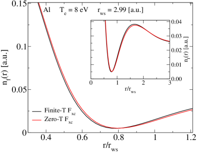
Figure 5: (Color online) The NPA free-electron density $n_{f}(r)$ for Al³⁺ at density $\rho=2.7$ g/cm³, with $T_{e}=8$ eV and $T_{i}=0.026$ eV, calculated using XC at finite-$T$ and at $T=0$. The inset shows the density for larger $r/r_{\text{ws}}$.

The finite-$T$ XCF is present in two contributions to the pressure, namely the electron-electron interacting linear response function $\chi(k,T_{e})$, which is used to construct the pseudopotential and the pair potential, and the HEG electron kinetic pressure. Although the finite-$T$ XCF has noticeable effects on the pair potentials or on the energy spectrum of bound states, we observe that overall thermodynamic effects are only slightly sensitive to such finite-$T$ corrections as can be seen in Fig. 6. In fact, at $T_{e}=8$ eV, the finite$-T$ XCF only decreases the pressure in Al by $4\%$. Since individual finite-$T$ contributions are considerable, this insensitivity to XCF comes from the interplay of several terms. For instance, the electron pressure by itself differs by about 10$\%$ in the regime $\theta\sim 0.8$, but the overall pressures obtained from $T=0$ and finite-$T$ NPA calculations differ by less than $4\%$.

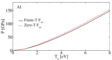
Figure 6: (Color online) Comparison between the pressure of Al in the UFM regime computed via the NPA model with the finite-$T$ $F_{xc}$ and with the zero-$T$ $F_{xc}$.

IV.4 Pseudopotential and mean ionization.

Here, we discuss the importance of choosing the proper pseudopotential for ab initio simulations of UFM systems in the $2T$ model. The pump-laser frequency is normally chosen such that core electrons are not excited and remain strongly bound to the ‘cold’ nuclei at temperature $T_{i}$. Thus, only the $\bar{Z}$ valence electrons on each ion are heated to $T_{e}$ during the irradiation. In DFT calculations, the electron temperature is used in a Fermi-Dirac distribution for the occupation numbers of all electrons in the simulation. Thus, if the chosen pseudopotential includes more electrons than the typical number of valence electrons, these core electrons will also be “heated” even if they should not in order to simulate correctly UFM systems. Wrong predictions may result, e.g., for the 2T pressure of the given UFM and its electronic specific heat.

To illustrate this point, we carried out ABINIT simulations using PAW pseudopotentials which include $\bar{Z}$=3 and 9 valence electrons for Li and Na, respectively. We also did NPA-DFT calculations with all electrons at $T_{e}$. In the NPA model, the mean ionization $\bar{Z}=Z_{n}-n_{b}$ can be computed as in Ref. PDW2 . The $\bar{Z}$ as a function of $T_{e}$ is not an integer in the NPA but represents an average over different ionization states as discussed in Ref. PDW95 .

In the case of Al and Li, the NPA predicts that $\bar{Z}$ is unaffected for $T_{e}<8$ eV, relevant to UFMs. Pressure should also be unchanged, which is exactly what we obtain with the ABINIT simulations of Li using the all-electron PAW pseudopotential. However, in the case of Na, $\bar{Z}$ starts to increase around $T_{e}=3$ eV up to $\bar{Z}=1.49$ at $T_{e}=8$ eV (see Table. 2). The increase in $\bar{Z}$ is accompanied by a decrease in the occupation of the 2$p$ level as electrons are promoted to the continuum. The decreased screening in the core (both due to increase of $T$ and due to the decrease in the number of core electrons) leads to a decrease in the radius of the $n$=2 shell. Hence, the increase of $\bar{Z}$ and the modification of the core levels do not lead to any ambiguity in specifying $\bar{Z}$.

Table 2: Mean ionization $\bar{Z}$, the 2$p$ Fermi factor, and the 2$p$ mean radius (a.u) for sodium (normal solid density) are given as a function of the temperature $T$ in eV. The WS radius $r_{ws}$=3.3912 a.u. and hence the core is compactly contained inside the WS sphere of Na for all values of $T$ investigated here.

$T$	$\bar{Z}$	$f_{2p}$	$<r_{2p}>$
1.00	1.001	1.000	0.808
3.00	1.004	0.999	0.804
5.00	1.104	0.983	0.792
8.00	1.494	0.919	0.762
10.0	1.786	0.872	0.744

We computed the pressure with the NPA model including the changed $\bar{Z}$ and compared it with the ABINIT simulations of Na using the nine-electron PAW pseudopotential. Results are presented in Fig. 7.

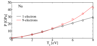
Figure 7: (Color online) Comparison between the pressure computed with the NPA (line) and with ABINIT (circles) when heating is applied to the valence electron of Na only or to all electrons (9 electrons in the ABINIT simulations).

We find that, at $T_{e}=8$ eV, the pressure, when heating of some core electrons is included, is $54\%$ higher than the correctly calculated value. The use of ‘all-electron’ codes for the study of UFM in the $2T$ state suffers from this pitfall of not selecting the physically appropriate $\bar{Z}$ and the corresponding pseudopotential. When suitable pseudopotentials are not available for DFT+MD calculations, one possibility is to use only the relevant part of the electron density of states (DOS) that is assigned to the free electrons on the basis of $\bar{Z}$, when pressure and related properties are computed. For instance, when calculating the specific heat of ‘free electrons’ for use in UFM studies, the ‘free-electron’ DOS used in the calculations should be consistent with the number of actual free electrons that couple with the laser. In a metal like gold (not studied here), even though a pseudopotential with 11 valence electrons is needed, the DOS used for evaluating the electron specific heat for $T_{e}<2$ should be only for $\bar{Z}=1$. The optical properties of gold (see ref. ChristyJon ) show that the $d$-shell couples to light only when the interband threshold energy ($\sim$ 2 eV) is exceeded. In the case of gold, the 5$d$ shell hybridizes with the continuum electrons (nominally made up of 6$s$ electrons) and extends outside the Au-Wigner-Seitz sphere until the $s-d$ transition threshold ($\sim$2 eV) is reached. Hence, at low temperatures the NPA model with its ‘one-center’ formulation cannot be used for gold at normal density. Similarly, WDM systems with bound states extending outside the Wigner-Seitz sphere cannot be treated unless explicit multi-center electron-ion correlation terms are included.

IV.5 Local pseudopotential for Li.

The Li pseudopotential used in the NPA is a local pseudopotential, whereas it is widely found in the context of large DFT codes that Li almost always needs a non-local pseudopotential. Even in early studies of phonons, a nonlocal pseudopotential was used by Dagens, Rasolt, and Taylor DRT , and yet the Li phonons at room temperature they obtained were less satisfactory than for, say, sodium. We have already shown that the NPA pair potential based on a local pseudopotential quite adequately reproduces the Li phonons at room temperature and high temperature at normal density, but not as accurately as for aluminum or sodium. Hence it is of interest to test the robustness of the Li pseudopotential and pair potential at higher compression by calculating the Li-Li $g(r)$ using the NPA potentials. Here we use the MHNC method where a bridge term is included using the Lado-Foiles-Ashcroft (LFA) criterion LFA-ChenLai92 which is based on the Gibbs-Bogoliubov inequality for the free energy of the system. The MHNC assumes radial symmetry and lim- its us to “simple-liquid” structures.

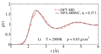
Figure 8: (Color online) The Li-Li NPA-MHNC pair distribution function $g(r)$ at 2000K (0.173 eV), $\rho=$ 0.85 g/cm³, compared with the $g(r)$ of Ref. kietzmann2008 .

Since Li becomes a complex liquid with clustering effects at high compressions bonev2008 , we consider a compression of $\sim 1.6$ and compute the PDF for Li at 0.85 g/cm² and at 2000K (0.173 eV) for which results are available from Kietzmann et al. kietzmann2008 . The LFA criterion yields a hard-sphere packing fraction $\eta=0.371$ to model the bridge function. The resulting NPA-MHNC $g(r)$ is displayed together with the $g(r)$ of Ref.  kietzmann2008 in Fig. 8. We find that the simple but state-dependent local pseudopotential constructed from the free-electron charge pileup at a Li nucleus is adequate to calculate phonons (i.e, requiring an accuracy of meV energies), as well as the Li-Li PDFs up to moderate compressions and high coupling constants $\Gamma$.

IV.6 Comparison between equilibrium WDM and UFM EOS.

In UFM, the internal pressure mainly results from the hot electron subsystem since ions remain close to their initial temperature $T_{r}$. Here, we investigate the difference in the pressure between the quasi-equilibrium UFM regime ($T_{i}\neq T_{e}$) and the equilibrium WDM regime which will usually be in a liquid or plasma state with $T_{i}=T_{e}$. In DFT codes it is possible to simulate liquids by computing forces among ions and the MD evolution of the positions of the $N$ ions in the simulation cell. However, to obtain reasonable statistics, one needs to use a supercell containing as many ions as possible, thus reducing considerably the first Brillouin zone and increasing the required number of electronic bands to be included. As mentioned earlier, the number of bands needs to be even larger in order to simulate $T_{e}$ via a Fermi-Dirac distribution. As examples, to obtain reasonably good band occupations for a system of 108 Al atoms at room density, 360 bands at $T_{e}=1$ eV are required, and this number grows to 1200 at $T_{e}=5$ eV. Thus, since computing repeatedly at every MD step a high number of bands in DFT codes is computationally very demanding, it becomes prohibitive at higher temperatures. Such a problem does not occur in the NPA model as only one DFT calculation at a single nucleus is required to construct the ion-ion pair potential. The structure factors may be computed using MD, or with MHNC equation for simple liquids.

The comparison of the pressure from UFM and equilibrium WDM is presented in Fig.  9. The equilibrium WDM pressure is much higher than the UFM value. Furthermore, the DFT-NPA calculation is in agreement with NPA up to $T_{e}=5$ eV (the limit of our DFT+MD simulation). This mutually reconfirms the validity of the NPA as well as DFT+MD approaches in the WDM regime.

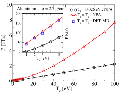
Figure 9: (Color online) Comparison of the NPA isochoric pressures for the UFM system and the equilibrium liquid system. Inset : Comparison of the NPA pressures in the low-$T$ regime where DFT+MD is practical.

Since $\bar{Z}$ reaches $\sim$ 7 at $T_{e}\sim$100 eV, codes for simulating Al should employ pseudopotentials that include more electrons than the 3 valence electrons valid at low temperatures. Simulations with high $\bar{Z}$ values will greatly increase the computational load and such calculations become prohibitive. Hence NPA methods or orbital-free Hohenberg-Kohn methods become relevant karaisev2014 . The latter do not however provide energy spectra and details of the bound electrons.

V Conclusion.

In order to describe physical properties of UFM, we examined applications of the NPA model within the two-temperature quasi-equilibrium model. We computed phonons, as well as the pressure resulting from the heating of free electrons. The excellent accord between such NPA calculations and DFT simulations using the ABINIT and VASP codes reconfirms the use of the NPA in this regime. As the internal pressure increases due to the heating of electrons by the ultrafast laser pulses, we explicitly showed that the phonon picture does not have much physical meaning, especially for thin WDM samples, even if frequencies could be computed using the harmonic approximation. As the NPA approach has negligible computational cost compared to standard DFT codes, it is a valuable tool for swiftly and accurately calculating important WDM properties such as mean ionization, pair potentials, structure factors, phonons, x-ray Thomson scattering spectra, electron-ion energy relaxation, conductivity, etc..

References

- (1) G. Dimonte and J. Daligault, Phys. Rev. Lett. 101, 135001 (2008).
- (2) See e.g. V. Mijoule, L. J. Lewis, and M. Meunier, Phys. Rev. A 73, 033203 (2006).
- (3) P. Lorazo, L. J. Lewis, and M. Meunier, Phys. Rev. Lett. 91, 225502 (2003); Phys. Rev. B 73, 134108 (2006).
- (4) Y. Ping, A.A. Correa, T. Ogitsu, E. Draeger, E. Schwegler, T. Aob, K. Widmanna, D.F. Price, E. Lee, H. Tamb, P.T. Springer, D. Hansonb, I. Koslowb, D. Prendergast, G. Collins and A. Ng, High Energy Density Physics 6, 246 (2010).
- (5) H. M. Milchberg, R. R. Freeman, S. C. Davey, and R. M. More, Phys. Rev. Lett. 61, 2364 (1988).
- (6) B. Chimier, V. Tikhonchuk, and L. Hallo, Phys. Rev. B 75, 195124 (2007).
- (7) L. Harbour, M. W. C. Dharma-wardana, D. Klug and L. Lewis, Physical Review E 94, 053211, (2016).
- (8) K. P. Driver and B. Militzer, Phys. Rev. Lett. 108, 115502 (2012).
- (9) Z. Chen, B. Holst, S. E. Kirkwood, V. Sametoglu, M. Reid, Y. Y. Tsui, V. Recoules, and A. Ng, Phys. Rev. Lett. 110, 135001 (2013).
- (10) N. Medvedev, U. Zastrau, E. Forster, D. O. Gericke, and B. Rethfeld, Phys. Rev. Lett. 107, 165003 (2011).
- (11) L. Dagens, J. Phys. C 5, 2333 (1972).
- (12) L. Dagens, J. Phys. (Paris) 36, 521 (1975).
- (13) F. Perrot, Phys. Rev. B 47, 570 (1993).
- (14) F. Perrot M. W. C. Dharma-wardana, Phys. Rev. E 52, 52,52 (1995).
- (15) M. W. C. Dharma-wardana and M. S. Murrilo, Phys. Rev. E 77, 026401 (2008).
- (16) M. S. Murillo, J. Weisheit, S. B. Hansen, and M. W. C. Dharma-wardana. Phys. Rev. E 87, 063113 (2013).
- (17) S. H. Glenzer and Ronald Redmer, Rev. Mod. Phys. 81 1625 (2009)
- (18) P. Hohenberg and W. Kohn. Phys. Rev. 136, B864 (1964).
- (19) W. Kohn and L. J. Sham, Phys. Rev. 140, A1133 (1965).
- (20) F. Perrot, Y. Furutani, and M. W. C. Dharma-wardana, Phys. Rev. A 41, 1096 (1990)
- (21) M. W. C. Dharma-wardana, preprint: http://arxiv.org/abs/1607.07511, (2016).
- (22) X. Gonze and C. Lee, Computer Phys. Commun. 180, 2582-2615 (2009).
- (23) G. Kresse and J. Furthmüller, Phys. Rev. B 54, 11169 (1996).
- (24) F. Perrot and M. W. C. Dharma-wardana, Phys Rev. A 30, 2619 (1984).
- (25) D. G. Kanhere, P. V. Panat, A. K. Rajagopal and J. Callaway, Phys. Rev. A 33, 490 (1986).
- (26) H. Iyeetomi and S. Ichimaru, Phys. Rev. A 34, 433 (1986).
- (27) F. Perrot and M. W. C. Dharma-wardana, Phys. Rev. B 62, 16536 (2000); Erratum: 67, 79901 (2003).
- (28) E. W. Brown, J. L. DuBois, M. Holzmann and D. M. Ceperley, Phys. Rev. 88, 081102 (2013).
- (29) V. V. Karasiev, T. Sjostrom, J. Dufty and S. B. Trickey, Phys. Rev. Lett. 112, 076403 (2014).
- (30) M. W. C. Dharma-wardana, Contrib. Plasma Phys. 55, No.2-3, 79-81 (2015)
- (31) J. M. Ziman, Proc. R. Soc., London 91, 701 (1967).
- (32) M. W. C. Dharma-wardana and F. Perrot, Phys. Rev. A 26, 4 (1982).
- (33) F. Perrot, Phys. Rev. A 42, 8 (1990).
- (34) M. W. C. Dharma-wardana, Phys. Rev. E 86, 036507 (2012).
- (35) M. W. C. Dharma-wardana and F. Perrot,in Density Functional Theory Eds. E. H. K. Gross, and R. M. Dreizler, NATO ASI series B: Physcs 337, p 625-650 Plenum, New York (1993).
- (36) S. B. Hansen et al., Phys. Rev. E 72, 036408 (2005); B. Wilson et al., J. Quant. Spectrosc. Radiat. Transfer 99, 658 (2006).
- (37) R. Piron and T. Blenski PRE 83, 026403 (2011).
- (38) T. Blenski, R. Piron, C. Caizergues, B. Cichocki, High Energy Density Physics, 9, 687-695 (2013)
- (39) C. E. Starrett and D. Saumon, Phys. Rev. E 87, 013104 (2013).
- (40) I. Tamblym, J.-Y. Raty and S. A. Bonev, Phys. Rev. Lett. 101, 075703 (2008).
- (41) R. W. Shaw and W. A. Harrison, Phys. Rev. 163, 604 (1967).
- (42) H. Wagenknecht, W. Ebeling, A. Förster,Contrib. Plasma Phys. 41, 15-25 (2001); Morita, T., Prog. Theor. Phys. 20 920, (1958).
- (43) N. W. Ashcroft and N. D. Mermin, Ch. 17, Eq. (17.42)-(17-55). Solid State Physics, Sanders College, Philadelpia, USA (1976); A. J. Archer, P. Hopkins, and R. Evans, Phys. Rev. E 74, 010402(R), (2006).
- (44) R. G. Gordon and Y. S. Kim, J. Chem. Phys. 56, 3122 (1972).
- (45) G. Faussurier, Physics of Plasmas 21(11), 112707 (2014).
- (46) J.-P. Hansen and I. R. McDonald, Theory of simple liquids Academic Press, San Diego, (1990).
- (47) N. W. Ashcroft and N. D. Mermin, Ch. 22, Solid State Physics, Sanders College, Philadelpia, USA (1976)
- (48) X. Gonze, Phys. Rev. B 55, 10337 (1997).
- (49) X. Gonze and C. Lee, Phys. Rev. B 55, 10355 (1997).
- (50) L. Harbour, M. W. C. Dharma-wardana, D. D. Klug, L.J. Lewis, Contr. Plasma. Phys. 55, 144 (2015).
- (51) V. Recoules, J. Clérouin, G. Zérah, P.M. Anglade, and S. Mazevet, Phys. Rev. Lett. 96, 055503 (2006).
- (52) P. B. Johnson and R. W. Christy, Phys. Rev. B 6, 4370 (1972).
- (53) L. Dagens, M. Rasolt and R. Taylor, Phys. Rev. B 11, 8 (1975).
- (54) H. C. Chen and S. K. Lai, Phys. Rev. A 45, 3831 (1992).
- (55) A. Kietzmann, R. Redmer, M. P. Desjarlais, and T. R. Mattson, Phys. Rev. Lett 101, 070401 (2008).
- (56) Valentin V. Karasiev, Travis Sjostrom, S.B. Trickey, Computer Physics Communications 185, 3240 (2014).