A Framework for Dynamic Stability Analysis of Power Systems with Volatile Wind Power

Abstract

We propose a framework employing stochastic differential equations to facilitate the long-term stability analysis of power grids with intermittent wind power generations. This framework takes into account the discrete dynamics which play a critical role in the long-term stability analysis, incorporates the model of wind speed with different probability distributions, and also develops an approximation methodology (by a deterministic hybrid model) for the stochastic hybrid model to reduce the computational burden brought about by the uncertainty of wind power. The theoretical and numerical studies show that a deterministic hybrid model can provide an accurate trajectory approximation and stability assessments for the stochastic hybrid model under mild conditions. In addition, we discuss the critical cases that the deterministic hybrid model fails and discover that these cases are caused by a violation of the proposed sufficient conditions. Such discussion complements the proposed framework and methodology and also reaffirms the importance of the stochastic hybrid model when the system operates close to its stability limit.

I introduction

Nowadays, many efforts have been devoted to producing the electric power from renewable energy sources among which the wind power is the most technically favorable and economically attractive [1]. However, volatile and uncontrollable characteristics of the wind power generation lead to stability concerns for the secure and economic operation of modern smart grids. As the wind penetration grows continuously, it is imperative to investigate the impacts of wind power generations on the system stability.

In the literature, the impacts of the wind power generation have been studied concerning different types of stabilities [2]-[8]. Specifically, [2]-[4] investigated the impacts of different parameters (e.g., the reactive power compensation, distance to the fault, and rotor inertia) on the transient and frequency stabilities of a power system; [5] addressed the influence of different wind generators on the transient stability; [1] and [6] studied the detrimental and beneficial influences of wind generators on transient and small-signal stabilities by converting wind generators to conventional synchronous generators; [7][8] analyzed the impacts of various control algorithms of wind generators on the long-term stability. In those studies, the variable nature of wind power is not considered and the wind speed is oversimplified as constant. To address this concern, [9]-[11] adopted an approach that describes the uncertainty of the wind power by stochastic differential equations (SDEs) and investigated the impacts of the wind generation on rotor-angle and small-signal stabilities, in which, however, the wind power was simply modeled as a Gaussian white noise perturbation on the power injection.

Regarding the long-term stability analysis that focuses on the time scale when fast dynamics damp out and control devices start working, however, a comprehensive framework is still missing in the literature to characterize the wind power with various stochastic properties, lay down a theoretical foundation for the stability assessment of these stochastic systems, and develop efficient numerical tools for such stability analysis. To address these issues, the Weibull model of the wind speed has been incorporated into the dynamic model of the power system to perform the long-term stability analysis [12], where SDEs are applied to describe the dynamics of the wind speed. By this SDE-based model, a theoretical approach that approximates the stochastic model by a deterministic model has been developed to reduce the computational burden caused by an accurate quantification of the uncertainty. Nevertheless, the proposed model and methodology are only applicable to continuous power system models. On the other hand, the discrete events induced by control and protective devices occur frequently in a long time scale after contingencies [13]. For instance, load tap changers are to restore the load-side voltages; shunt compensation switchings act to increase the transmission capability; and OvereXcitation Limiters may be activated to protect the generators from overheating. These discrete dynamics are generally designed to act after the fast dynamics damp out so as to avoid unnecessary interactions with the fast dynamics [13]-[15], and they require accurate representation by discrete models in time-domain simulation [16]. As a result, it is imperative to integrate discrete models to perform the comprehensive long-term stability analysis for realistic power systems.

The paper begins by showing that a power grid integrating wind power generations can be modeled as a stochastic hybrid model (SHM), with discrete dynamics, in a SDE-based framework in which the wind speed model that captures various stochastic properties can be integrated. In particular, it is analytically shown in this framework that SHM can be approximated by a deterministic hybrid model (DHM) which offers an accurate trajectory approximation (for SHM) and stability assessments with high computational efficiency if some mild sufficient conditions are satisfied. A numerical example is presented to demonstrate the accuracy and efficiency of DHM. It is noteworthy that SHM must be implemented whenever any proposed sufficient conditions are violated. To show this necessity, we present several numerical examples in which DHM fails to capture the instabilities of SHM. The causes for the failure are investigated and shown to correspond to a violation of the sufficient conditions. This discussion complements the proposed SDE-based framework, shows the application scope of the approximation methodology, and also emphasizes the largely-neglected necessity of the stochastic model in the long-term stability analysis.

As the modern smart grids endeavor to incorporate high penetration of intermittent renewable energy, integrate plug-in vehicles, and encourage opportunistic users, the operation and control of power grids are required to account for the resulting high variability and uncertainty. We believe that the proposed SDE-based framework and approximation methodology can be readily generalized to conduct stability assessments for power systems with the uncertainties brought about by various renewable energy sources, plug-in vehicles, smart appliances, opportunistic users, and so forth.

The remainder of the paper is organized as follows. Section II introduces the SDE-based framework of power system models integrating the stochastic dynamics of the wind speed. Section III develops an approximation methodology for SHM in the SDE-based framework, which provides an accurate trajectory approximation and correct stability assessments with a high simulation speed. In particular, a diagram is summarized at the end of Section III-A to illustrate the relationships among the proposed models and theoretical results. Furthermore, Section IV presents some critical cases in which some sufficient conditions of the proposed methodology are violated, to explain the necessity of implementing SHM to obtain correct stability assessments.

II sde-based framework of hybrid models

The conventional long-term stability model (i.e., the complete dynamic model) without stochasticity for simulating the system dynamic response to a disturbance in the $\tau$ time scale can be described as follows (see (22)-(25) [12] and (15) [17]):

$$\bm{{z}_{d}}(k) = \bm{{h}_{d}}(\bm{z_{c},x,y,z_{d}}(k-1))$$ (1)

$$\bm{{z}_{c}^{\prime}} = \bm{{h}_{c}({z_{c},x,y,z_{d}})}$$ (2)

$$\epsilon\bm{{{x}^{\prime}}} = \bm{f({z_{c},x,y,z_{d}})}$$ (3)

$$\bm{0} = \bm{g({z_{c},x,y,z_{d}})}$$ (4)

where $\tau=t\epsilon$ and $\prime$ refers to $\frac{d}{d\tau}$. Here, (1) accounts for the long-term discrete events, such as shunt capacitors and load tap changers (LTCs); (2) depicts the slow dynamics, including self restorative loads, turbine governors (TGs), and OvereXcitation Limiters (OXLs); (3) describes the fast dynamics of components, such as synchronous machines, doubly-fed induction generators (DFIGs), induction motors, and exciters; and (4) describes the power flow relation and internal relationships between variables. In addition, $\bm{h_{d}}$ are discrete functions; $\bm{z_{d}}$ are slow discrete variables whose changing from $\bm{z_{d}}(k-1)$ to $\bm{z_{d}}(k)$ relies on (1) and occurs at times $t_{k}$, $1\leq k\leq N$. The functions $\bm{{h}_{c}}$, $\bm{{f}}$, and $\bm{{g}}$ are continuous; $\bm{z_{c}}$, $\bm{{x}}$, and $\bm{{y}}$ are the vectors of slow state variables, fast state variables, and algebraic variables, respectively; and $\epsilon$ is deemed as the reciprocal of the maximum time constant among all components.

II-A Stochastic Model of Wind Speed

The impacts of the wind power on the system stability have been addressed [2]-[8] in which the wind speed is termed as a constant and an entry of the vector $\bm{y}$—algebraic variables. In this paper, we characterize the randomness of the wind speed by a stochastic model.

Specifically, given $n_{w}$ independent wind energy sources that each energy source follows a certain probability distribution, the wind speeds of the $n_{w}$ sources are collectively denoted by a vector $\bm{y_{w}}$ in the following model (see [12] and [18]):

$$\epsilon\bm{\eta_{w}}^{\prime} = -A\bm{\eta_{w}}+\sigma\bm{\xi}={\bm{f_{w}}(\bm{\eta_{w}})+\sigma\bm{{\xi}}},$$ (5)

$$\bm{y_{w}} = \bm{\hat{F}_{w}^{-1}}\left(\bm{\hat{\Phi}}\big{(}\tfrac{\bm{\eta_{w}}}{\sigma/\sqrt{2\bm{\alpha}}}\big{)}\right)=\bm{g_{w}(\eta_{w})},$$ (6)

where $\bm{\eta_{w}},\bm{y_{w}}\in\mathbb{R}^{n_{w}}$, the matrix

$$A=\mbox{diag}(\bm{\alpha})=\mbox{diag}[\alpha_{1},\ldots,\alpha_{n_{w}}]\in\mathbb{R}^{{n_{w}}\times{n_{w}}}$$

determines the autocorrelation property of $\bm{y_{w}}$ (see below for more details), and $\int_{0}^{t}\bm{\xi}(s)ds$ is an $n_{w}$-dimensional Wiener process. In addition, $\bm{\hat{F}_{w}}=[F_{1}(\eta_{w_{1}}),F_{2}(\eta_{w_{2}}),...F_{n_{w}}(\eta_{w_{n_{w}}})]^{T}$, $\bm{\hat{\Phi}}=[\Phi(\eta_{w_{1}}),\Phi(\eta_{w_{2}}),...\Phi(\eta_{w_{n_{w}}})]^{T}$, and $\bm{g_{w}}:\mathbb{R}^{n_{w}}\mapsto\mathbb{R}^{n_{w}}$, where $F_{i}$ is the cumulative distribution function of the corresponding wind speed $y_{w_{i}}$, and $\Phi$ is the cumulative distribution function of a Gaussian distribution.

In model (5)-(6) of the wind speed, $\bm{\eta_{w}}$ is a vector Ornstein-Uhlenbeck process, and each $y_{w_{i}}$ matches the distribution of $F_{i}$ by the property of the memoryless transformation [18]. For example, if the wind speed of source $n_{w_{i}}$ is governed by the Weibull distribution with a shape parameter $k_{i}>0$ and a scale parameter $\lambda_{i}>0$, then

$$F_{w_{i}}(u)={{1-e^{(u/\lambda_{i})^{k_{i}}}}}~{}\hbox{for all}~{}u>0,$$ (7)

and $y_{w_{i}}$ has the following statistical properties (see (26)-(28)[18]):

1. $\mathrm{E}[{y_{w_{i}}}(t)]={\lambda_{i}}\Gamma(1+\frac{1}{{k_{i}}})={\mu_{w_{i}}}$.

2. $\mathrm{Var}[{y_{w_{i}}}(t)]={\lambda_{i}}^{2}\Gamma(1+\frac{2}{{k_{i}}})-\mu_{w_{i}}^{2}$.

3. $\mathrm{Aut}[{y_{w_{i}}}(t_{k}),{y_{w_{i}}}(t_{j})]\approx e^{-\alpha_{i}|t_{j}-t_{k}|}$.

Note that $\lambda_{i}$, $k_{i}$, and $\alpha_{i}$ are the parameters that determine the statistical properties of wind speed $y_{w_{i}}$, but $\sigma$ does not. So $\sigma$ can be arbitrarily selected [12][18]. Indeed, $\sigma$ is only an intermediate parameter to generate the Ornstein-Uhlenbeck process $\bm{\eta_{w}}$. The readers are referred to [18] for more details.

II-B Hybrid Models

When integrating the stochastic model (5)-(6) of the wind speed into the long-term stability model (1)-(4), the stochastic hybrid model (SHM) takes the following form:

$$\bm{{z}_{d}}(k) = \bm{\bar{h}_{d}(\bm{z_{c}},\bm{\bar{x}},\bm{\bar{y}},}\bm{z_{d}}(k-1)\bm{)},$$ (8)

$$\bm{{z}_{c}}^{\prime} = \bm{\bar{h}_{c}({\bm{z_{c}},\bm{\bar{x}},\bm{\bar{y}},\bm{z_{d}}})},$$ (9)

$$\epsilon{\bm{\bar{x}}}^{\prime} = \bm{\bar{f}({\bm{z_{c}},\bm{\bar{x}},\bm{\bar{y}},\bm{z_{d}}})}+\sigma B\bm{\bar{\xi}},$$ (10)

$$\bm{0} = \bm{\bar{g}({\bm{z_{c}},\bm{\bar{x}},\bm{\bar{y}},\bm{z_{d}}})},$$ (11)

where $\bm{\bar{x}}\doteq\left[\begin{smallmatrix}\bm{x}\\ \bm{\eta_{w}}\end{smallmatrix}\right]$, $\bm{\bar{y}}\doteq\left[\begin{smallmatrix}\bm{y}\\ \bm{y_{w}}\end{smallmatrix}\right]$, and $B\doteq\left[\begin{smallmatrix}0\\ I_{n_{w}}\end{smallmatrix}\right]$, nonzero entries of which correspond to $n_{w}$ independent wind sources. In addition, $\bm{\bar{f}}\doteq\left[\begin{smallmatrix}\bm{f}\\ \bm{f_{w}}\end{smallmatrix}\right]$, $\bm{\bar{g}}\doteq\left[\begin{smallmatrix}\bm{g}\\ \bm{p}\end{smallmatrix}\right]$ with $\bm{p}\doteq\bm{y_{w}}-\bm{g_{w}(\eta_{w})}$, and $\bar{\bm{\xi}}=\left[\begin{smallmatrix}0\\ {\bm{\xi}}\end{smallmatrix}\right]\in\mathbb{R}^{{n_{x}}\times{n_{w}}}$. Here, (8) and (9) are directly derived from (1) and (2), respectively, such that $\bm{\bar{h}_{d}(\bm{z_{c}},\bm{\bar{x}},\bm{\bar{y}},}\bm{z_{d}}(k-1)\bm{)}=\bm{{h}_{d}}(\bm{z_{c},x,y,z_{d}}(k-1))$ and $\bm{\bar{h}_{c}({\bm{z_{c}},\bm{\bar{x}},\bm{\bar{y}},\bm{z_{d}}})}=\bm{{h}_{c}({z_{c},x,y,z_{d}})}$; (10) is obtained from a combination of (3) and (5), whereas (11) is derived by combining (4) and (6).

Recall that discrete dynamics described by (8) play important roles in the long-term stability because many protective and control devices may take effect in the long-term time scale to restore the load-sided power, protect generators, and so on.

This study aims to show that the SHM (8)-(11) can be well approximated by a deterministic hybrid model (DHM), say,

$$\bm{{z}_{d}}(k) = \bm{\bar{h}_{d}(\bm{z_{c}},\bm{\bar{x}},\bm{\bar{y}},}\bm{z_{d}}(k-1)\bm{)},$$ (12)

$$\bm{{z}_{c}}^{\prime} = \bm{\bar{h}_{c}({\bm{z_{c}},\bm{\bar{x}},\bm{\bar{y}},\bm{z_{d}}})},$$ (13)

$$\epsilon{\bm{\bar{x}}}^{\prime} = \bm{\bar{f}({\bm{z_{c}},\bm{\bar{x}},\bm{\bar{y}},\bm{z_{d}}})},$$ (14)

$$\bm{0} = \bm{\bar{g}({\bm{z_{c}},\bm{\bar{x}},\bm{\bar{y}},\bm{z_{d}}})}.$$ (15)

Note that the vector of algebraic variables $\bm{\bar{y}}$ in (11) and (15) can be eliminated under Assumption 1 which is a generic property satisfied in normal operating conditions [13][19].

Assumption 1. The DHM (12)-(15) does not encounter singularity, i.e., $\frac{\partial{\bm{\bar{g}}}}{\partial{\bm{y}}}$ is nonsingular along the trajectory.

Under Assumption 1, $\bm{\bar{y}}$ can be represented in terms of $\bm{z_{c}}$, $\bm{\bar{x}}$, and $\bm{z_{d}}$ using (15), namely $\bm{\bar{y}=m(\bm{z_{c}},\bm{\bar{x}},\bm{z_{d}})}$. Then, the SHM (8)-(11) can be written as:

$$\bm{z_{d}}(k) = \bm{H_{d}(\bm{z_{c}},\bm{\bar{x}},}\bm{z_{d}}(k-1)\bm{)},$$ (16)

$$\bm{z_{c}}^{\prime} = \bm{H_{c}(\bm{z_{c}},\bm{\bar{x}},\bm{z_{d}})},$$ (17)

$$\epsilon\bm{\bar{x}}^{\prime} = \bm{F(\bm{z_{c}},\bm{\bar{x}},\bm{z_{d}})}+\sigma B{\bm{\bar{\xi}}}.$$ (18)

By analogy, the DHM (12)-(15) is equivalently converted to:

$$\bm{z_{d}}(k) = \bm{H_{d}(\bm{z_{c}},\bm{\bar{x}},}\bm{z_{d}}(k-1)\bm{)},$$ (19)

$$\bm{z_{c}}^{\prime} = \bm{H_{c}(\bm{z_{c}},\bm{\bar{x}},\bm{z_{d}})},$$ (20)

$$\epsilon\bm{\bar{x}}^{\prime} = \bm{F(\bm{z_{c}},\bm{\bar{x}},\bm{z_{d}})}.$$ (21)

In section III, a theoretical foundation is to be developed to ensure the effectiveness of the approach that approximates the SHM (16)-(18) by the DHM (19)-(21) in the long-term stability study. The key is to show that if some mild conditions are satisfied, then the DHM (19)-(21) is theoretically ensured to provide an accurate trajectory approximation and stability assessments for the SHM (16)-(18). Clearly, the DHM consumes much less computational resources in the simulation compared with the SHM and may serve as an efficient stability assessment tool for power grids with significant wind power generations.

III an approximation methodology for stochastic hybrid model

The singular perturbation method for SDEs [20]-[22] and sufficient conditions for the quasi steady-state (QSS) model [17][23] are employed here to develop a theoretical foundation for an approximation of the SHM (16)-(18) by the DHM (19)-(21). A numerical example using a 145-bus system is presented to demonstrate the accuracy and efficiency of the DHM.

III-A Theoretical Foundation

In the SHM, when the discrete jumping is initiated, discrete variables $\bm{z_{d}}$ are updated first by (16), and then the system acts according to (17)-(18) with constant $\bm{z_{d}}$. In this regard, one can treat the SHM (16)-(18) as a series of continuous systems (17)-(18) with constant $\bm{z_{d}}$ [13]. Similarly, the DHM (19)-(21) can be considered as a series of continuous systems (20)-(21) with constant $\bm{z_{d}}$. It is reasonable to assume that the SHM and the DHM are governed by the same sequence of parameter values $\bm{z_{d}}$ given the same initial condition. So, the hybrid models (i.e., SHM and DHM) can be analyzed by comparing the corresponding continuous systems in the series. Additionally, we suppose that each deterministic continuous system (20)-(21) satisfies some generic differentiability and non-degeneracy conditions (see Assumption 2.1 [12]), which are reasonable assumptions for real-life physical systems.

If $\bm{\bar{x}}={\bm{m_{1}(\bm{z_{c}},\bm{z_{d}})}}$ is an asymptotically stable equilibrium point of the short-term stability model $\bm{0}=\bm{F(\bm{z_{c}},\bm{\bar{x}},\bm{z_{d}})}$ for all $\bm{z_{c}}$ and $\bm{z_{d}}$, i.e., $\bm{\bar{x}}=\bm{m_{1}(\bm{z_{c}},\bm{z_{d}})}$ is a stable component of the constraint manifold, then there exists an invariant manifold of system (19)-(21): $\bm{\bar{x}}=\bm{m_{1}^{\star}}(\bm{z_{c}},\bm{z_{d}},\epsilon)=\bm{m_{1}(\bm{z_{c}},\bm{z_{d}})}+O(\epsilon)$ for sufficiently small $\epsilon$ [12][24][25], where $\bm{m_{1}(\bm{z_{c}},\bm{z_{d}})}$ and $\bm{m_{1}^{\star}}(\bm{z_{c}},\bm{z_{d}},\epsilon)$ can be not smooth. An ellipsoidal layer ${M}(h)$ around $\bm{m_{1}^{\star}}(\bm{z_{c}},\bm{z_{d}},\epsilon)$ is defined as follows:

$${M}(h) \doteq \{(\bm{z_{c}},\bm{\bar{x}},\bm{z_{d}}):\langle(\bm{\bar{x}}-\bm{m_{1}}^{\star}(\bm{z_{c}},\bm{z_{d}},\epsilon)),$$

$$\quad M_{1}^{\star}(\bm{z_{c}},\bm{z_{d}},\epsilon)^{-1}(\bm{\bar{x}}-\bm{m_{1}^{\star}}(\bm{z_{c}},\bm{z_{d}},\epsilon))\rangle<h^{2}\}.$$

Here, the matrix $M_{1}^{\star}(\bm{z_{c}},\bm{z_{d}},\epsilon)$ that represents the cross section of $M(h)$ is properly defined (see Appendix B in [12]), and an illustration for $M(h)$ is shown in Fig. 1.

Figure 1: An illustrtion of $M(h)$ in the DHM. Here, $n_{z_{c}}=1$, $n_{\bar{x}}=2$, and $M(h)$ is an ellipsoidal layer around $\bm{m_{1}^{\star}}(\bm{z_{c}},\bm{z_{d}},\epsilon)$.

Given the well-defined initial condition for each continuous system (17)-(18) with constant $\bm{z_{d}}$ (of the SHM), the following theorem shows that the trajectories of the SHM (16)-(18) are confined in $M(h)$ despite the changes of discrete variables, provided that the slow manifold is stable.

Theorem 1 (Sample-Path Concentration for SHM):
Consider the SHM (16)-(18) in the study region $D_{\bm{z_{d}}}\times D_{\bm{z_{c}}}\times D_{\bm{x}}$, for some fixed $\epsilon_{0}>0$, $h_{0}>0$, there exist $\delta_{0}>0$, a time $\tilde{\tau}_{k}$ of order $\epsilon|\mbox{log}h|$, and $\tau_{k}>\tilde{\tau}_{k}$ for each continuous system (17)-(18) with $0\leq k\leq N$ such that if the following conditions (i) and (ii) are satisfied:

(i)

The slow manifold $\bm{\bar{x}}=\bm{m_{1}(\bm{z_{c}},\bm{z_{d}})}$ is a stable component of the constraint manifold, where $\bm{z_{c}}\in D_{\bm{z_{c}}}$ and $\bm{z_{d}}\in D_{\bm{z_{d}}}$;

(ii)

The initial condition $(\bm{z_{c}}^{k}(0),\bm{\bar{x}}^{k}(0),\bm{z_{d}}(k))$ for each continuous system (17)-(18) of the SHM satisfies that $(\bm{z_{c}}^{k}(0),\bm{\bar{x}}^{k}(0),\bm{z_{d}}(k))\in M(\delta_{0})$, where $\bm{z_{c}}^{k}(0)\in D_{\bm{z_{c}}}$ and $\bm{z_{d}}(k)\in D_{\bm{z_{d}}}$ for $k\in[0,1,...N]$,

then, for all $\tau\in\Pi=\cup_{i=1}^{N-1}[\tilde{\tau}_{i},\tau_{i})\cup[\tilde{\tau}_{N},\infty]$, the sample path $(\bm{z_{c}}(\tau),\bm{\bar{x}}(\tau),\bm{z_{d}}(\tau))$ of the SHM (16)-(18) satisfies the following probability property:

$$\mathbb{P}\{\exists\,\tau\in\Pi: (\bm{z_{c}}(\tau),\bm{\bar{x}}(\tau),\bm{z_{d}}(\tau))\notin M(h)\}$$ (22)

$$\leq C_{n_{z_{c}},n_{x}}(\tau,\epsilon)e^{\frac{-h^{2}}{2\sigma^{2}}(1-O(h)-O(\epsilon))},$$

for all $\epsilon\leq\epsilon_{0}$, $h\leq h_{0}$, where the coefficient $C_{n_{z_{c}},n_{x}}(\tau,\epsilon)=[C^{n_{z_{c}}}+h^{-n_{x}}](1+\frac{\tau}{\epsilon^{2}})$ is linear in $\tau$.

Proof: See Appendix A.

Theorem 1 shows that if conditions (i)-(ii) are satisfied, then the probability that the sample path leaves $M(h)$ is less than the right hand side (RHS) of (22). Specifically, if $h\gg\sigma$, i.e., the deepness of the layer $h$ is far larger than $\sigma$ related with wind speeds, then the RHS of (22) becomes very small, which suggests that the sample pathes of the SHM do not leave $M(h)$ almost surely [12][20]. So, there is no need to worry about the probability when investigating the relations between the trajectory of the SHM (16)-(18) and that of the DHM (19)-(21). On the other hand, $\sigma$ does not influence the stochastic properties of wind speed $\bm{y_{w}}$ as stated in Section II-A or Section III-A in [12] (where $\sigma$ is only an intermediate parameter to generate the Ornstein-Uhlenbeck process $\bm{\eta_{w}}$). In this regard, $\sigma$ can be selected as small as needed such that any adequate $h$ satisfies $h\gg\sigma$. In other words, the requirement $h\gg\sigma$ can be readily fulfilled in this SDE-based framework. In addition, Theorem 2.4 [21] has commented that for $h\gg\sigma$, the first exit time that the solution $\bm{z_{c}}$ of the (continuous) stochastic system (17) leaves the region $D_{\bm{z_{c}}}$ is very large (exponentially in $h^{2}/\sigma^{2}$), that is, $\bm{z_{c}}$ still stays within $D_{\bm{z_{c}}}$ almost for sure right before the (discrete) change of $\bm{z_{d}}$ occurs at $t_{k}$. Note that, for adequately controlled systems, discrete devices generally do not result in severe perturbations to the system dynamics. So, these facts suggest that condition (ii) in Theorem 1 is generally satisfied under normal operating conditions.

Under the condition $h\gg\sigma$, we next investigate the relationship between the trajectory of the SHM (16)-(18) and that of the DHM (19)-(21). If (a) the trajectory of the SHM remains in $M(h)$ which is an $\epsilon$ neighborhood of the invariant manifold $\bm{m_{1}^{\star}}(\bm{z_{c}},\bm{z_{d}},\epsilon)$, and (b) the trajectory of the DHM evolves along $\bm{m_{1}^{\star}}(\bm{z_{c}},\bm{z_{d}},\epsilon)$, then we show that the distance between the trajectory of the SHM and that of the DHM can be readily obtained. Note that Theorem 1 provides sufficient conditions for (a). So, the remaining question is about how to ensure (b). Incidentally, the theoretical foundation for the quasi steady-state (QSS) model in [17] has provided sufficient conditions for (b). In particular, one of the sufficient conditions for (b) is the condition of consistent attraction defined below and illustrated in Fig. 2.

Definition 1. Consistent Attraction [17]: By fixing $\bm{z_{c}}$ and $\bm{z_{d}}$ as the parameters, the short-term stability model refers to (21). We say that the DHM (19)-(21) satisfies the condition of consistent attraction if the initial condition is contained in the stability region of the initial short-term stability model and whenever discrete variables jump from $\bm{z_{d}}(k-1)$ to $\bm{z_{d}}(k)$, $k=1,2,...,N$, the point on trajectory of the DHM immediately after $\bm{z_{d}}$ jump still stays within the stability region of the corresponding short-term stability model.

Figure 2: The situation when the DHM satisfies the condition of consistent attraction.

The condition of consistent attraction ensures that the trajectory of the DHM is always close to the slow manifold $\bm{m_{1}(\bm{z_{c},z_{d}})}$ despite the changing of discrete variables (if the slow manifold is also stable), then the trajectory of the DHM always evolves along the invariant manifold $\bm{m_{1}^{\star}}(\bm{z_{c}},\bm{z_{d}},\epsilon)$. Let $(\bm{z_{c}}(\tau),\bm{\bar{x}}(\tau),\bm{z_{d}}(\tau))$ be the trajectory of the SHM (16)-(18), and let $(\bm{z_{cD}}(\tau),\bm{\bar{x}_{D}}(\tau),\bm{z_{d}}(\tau))$ be that of the DHM (19)-(21). Then, the following theorem reveals the relationship between the trajectories of the two models.

Theorem 2 (Trajectory Relationship for Hybrid Models):
Given $h\gg\sigma$, consider the SHM (16)-(18) and the DHM (19)-(21) in the study region $D_{\bm{z_{d}}}\times D_{\bm{z_{c}}}\times D_{\bm{x}}$, for some fixed $\epsilon_{0}\in(0,h)$, there exist $\delta_{0}>0$, a time $\tilde{\tau}_{k}$ of order $\epsilon|\mbox{log}h|$ and $\bar{\tau}_{k}>\tilde{\tau}_{k}$ for each continuous system (17)-(18) where $k=0,1,...,N$, such that if the following conditions (i), (ii) and (iii) are satisfied:

(i)

The slow manifold $\bm{\bar{x}}=\bm{m_{1}(\bm{z_{c}},\bm{z_{d}})}$ is a stable component of the constraint manifold, where $\bm{z_{c}}\in D_{\bm{z_{c}}}$ and $\bm{z_{d}}\in D_{\bm{z_{d}}}$;

(ii)

The initial condition $(\bm{z_{c}}^{k}(0),\bm{\bar{x}}^{k}(0),\bm{z_{d}}(k))$ for each continuous system (16)-(18) of the SHM satisfies $(\bm{z_{c}}^{k}(0),\bm{\bar{x}}^{k}(0),\bm{z_{d}}(k))\in M(\delta_{0})$, where $\bm{z_{c}}^{k}(0)\in D_{\bm{z_{c}}}$ and $\bm{z_{d}}(k)\in D_{\bm{z_{d}}}$ for $k\in[0,1,...N]$;

(iii)

The DHM (19)-(21) satisfies the condition of consistent attraction,

then, for $\tau\in\cup_{i=1}^{N}[\tilde{\tau}_{i},\bar{\tau}_{i}]$, the following relations hold:

$$|\bm{\bar{x}}(\tau)-\bm{\bar{x}_{D}}(\tau)| = O(\sigma),$$ (23)

$$|\bm{z_{c}}(\tau)-\bm{z_{cD}}(\tau)| = O(\sigma\sqrt{\epsilon}),$$ (24)

for all $\epsilon\in(0,\epsilon_{0})$.

Proof: See Appendix B.

By Theorem 2 we observe that if the proposed sufficient conditions are satisfied, the trajectory of the SHM can be approximated by that of the DHM as illustrated in Fig. 3.

Figure 3: The trajectory $\phi_{s}(\tau,\bm{z_{c}}(0),\bm{\bar{x}}(0),\bm{z_{d}})$ of SHM is bounded in $M(\sigma)$, and can be estimated by the trajectory $\phi_{l}(\tau,\bm{z_{c}}(0),\bm{\bar{x}}_{D}(0),\bm{z_{d}})$ of DHM.

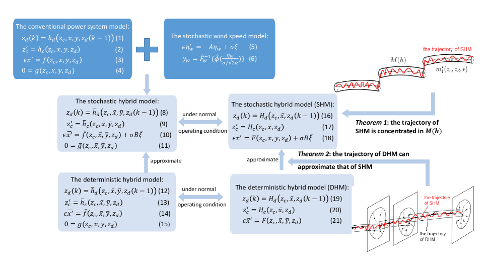
Figure 4: The proposed SDE-based framework and the approximation methodology.

Generally speaking, sufficient conditions (i)-(iii) in Theorem 2 are moderate and satisfied when the system operates away from the stability boundary, and thus the DHM can substitute the SHM and typically offer correct stability assessments with less simulation time. But, as detailed in Section IV, the SHM must be applied if any of the sufficient conditions is violated.

For clarity, we summarize in Fig. 4 the proposed SDE-based framework, relationship between different models, and importance of derived theoretical results. In the SDE-based framework, the stochastic model (5)-(6) of the wind speed is incorporated into the conventional power system model (1)-(4), and the resulting hybrid model (8)-(11) is equivalent to the SHM (16)-(18) under normal operating condition. Specifically, Theorem 1-2 shows that the DHM (19)-(21) can well approximate the SHM (16)-(18). In particular, Theorem 1 suggests that the sample paths of (16)-(18) are concentrated in a neighborhood $M(h)$ of the invariant manifold $\bm{m_{1}^{\star}}(\bm{z_{c}},\bm{z_{d}},\epsilon)$, while Theorem 2 asserts that the DHM (19)-(21) can provide an accurate trajectory approximation and stability assessments for the SHM (16)-(18) under some mild conditions. So, under normal operating conditions and the proposed mild conditions, the DHM (12)-(15) can well approximate the SHM (8)-(11) in terms of the trajectory and stability assessments.

III-B Numerical Illustration

Numerical studies using a 145-bus test case [26] are conducted in PSAT-2.1.8 [27] to show the accuracy and efficiency of the derived results. The test system has 6 doubly-fed induction generators (DFIGs) driven by 6 independent Weibull-distributed wind sources. The parameters of Weibull distributions are referred from [18] which fit the 1-h wind speed data of the Cape St. James and Victoria Airport. The readers are referred to Table 1 [18] for more details. In addition, there are 50 synchronous generators (GENs) with automatic voltage regulators (AVRs). Turbine governors (TGs) are equipped for GEN 10-GEN 20, and OvereXcitation Limiters (OXLs) are also equipped for GEN 1-GEN 6. The initial time delays of OXLs are 50s. Moreover, 5 discrete load tap changers (LTCs) are installed at Bus 79-95, Bus 1-33, Bus 79-92, Bus 1-5, and Bus 60-95, respectively. Particularly, the discrete model of LTCs is shown below [15]:

$$n(k+1)=\left\{\begin{array}[]{ll}n(k)+\triangle{n},&\mbox{if }v>v_{0}+d\mbox{ and }n(k)<n^{max};\\ n(k)-\triangle{n},&\mbox{if }v<v_{0}-d\mbox{ and }n(k)>n^{min};\\ n(k),&\mbox{otherwise};\end{array}\right.$$ (25)

where $n$ is the tap changer ratio, $v$ is the controlled voltage, $v_{0}$ is the reference voltage, $d$ is half of the LTC dead-band, $n^{max}$ and $n^{min}$ are the upper and lower tap limits, respectively. All LTCs have initial time delays of 50s and fixed tapping delays of 10s. At 0.5s, three lines at Bus 95-138, Bus 94-138, Bus 94-95 trip.

Note that the dynamic models for synchronous generators and DFIGs used in this and subsequent numerical examples are all detailed in Ch. 17 and Ch. 21 [28]. Specifically, the order II and order IV models of GENs are employed for the simulation of this 145-bus system.

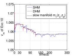
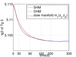
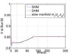
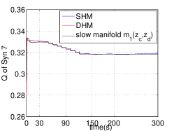
Figure 5: A comparison of the trajectory of the SHM and that of the DHM by simulating the 145-bus system.

Fig. 5 presents a comparison of the trajectory of the SHM and that of the DHM for which the quasi steady-state (QSS) model [13] is implemented to obtain the slow manifolds of the DHM. Observe that the trajectories of the SHM always keep close to those of the DHM despite the changing of discrete variables, and both models give the same stability assessments that the system is stable in the long-term time scale. Clearly, all sufficient conditions of Theorem 2 are satisfied, then the conclusions of Theorem 2 hold. Particularly, Fig. 5 shows that the DHM does not encounter the singularity and its slow manifold is stable. In addition, the trajectory of the DHM evolves along $\bm{m_{1}^{\star}}(\bm{z_{c}},\bm{z_{d}},\epsilon)$ which is an $\epsilon$-neighborhood of the slow manifold. This illustrates the results of Theorem 2.

Concerning the computational efficiency, the SHM takes 137.118s to complete the simulation, whereas the DHM only consumes 57.913s. Note that several trajectories of the SHM may be required to evaluate the stability in critical cases. But, the time needed to simulate one trajectory (of the SHM) can be more than twice as that required by the DHM.

From this example, we observe that the DHM can provide an accurate trajectory approximation and stability assessments for the SHM with far less simulation time, provided that the proposed mild conditions are satisfied.

IV necessity of stochastic model

A comprehensive theoretical framework has been developed to approximate the SHM by the DHM. Specifically, if all sufficient conditions of Theorem 2 are satisfied, then the DHM can provide an accurate trajectory approximation and stability assessments for the SHM with much less simulation time. In the section, we further present several examples in critical cases that the DHM fails to provide a satisfactory approximation. The causes for such failure are investigated in the nonlinear system framework and are shown to correspond to a violation of the proposed sufficient conditions. This discussion complements the proposed framework and methodology and also highlights the necessity of the stochastic model when performing the stability analysis for the power system with significant wind power generations, especially for the system that operates close to the stability boundary. Given the importance of such sufficient conditions, it is imperative to develop efficient numerical algorithms to check these conditions in the near future.

IV-A Numerical Example I

This example is a modified IEEE 14-bus system. The order V and order VI models of GENs are employed. A Weibull-distributed wind source drives a DFIG at Bus 2, and 3 GENs are equipped with AVRs and TGs. In addition, 3 exponential recovery loads (ERLs) are at Bus 9, 10, and 14, respectively. An OXL is installed for GEN 1, and 3 discrete LTCs are at Bus 4-9, Bus 12-13 and Bus 2-4, respectively, the initial time delays of which are 30s and fixed tapping delays are 10s. At 1s, three lines at Bus 6-13, Bus 7-9, and Bus 6-11 trip. We refer the reader to Appendix C for the parameter values.

A comparison between the trajectory of the DHM and that of the SHM is shown in Fig. 6. The slow manifold of the DHM acquired from the QSS model is also illustrated. The DHM converges to a long-term stable equilibrium point (SEP) with all voltages in the nominal range, which shows that the DHM is long-term stable. But, the sample path of the SHM suffers from a voltage collapse. So, the DHM fails to provide a stability assessment agreeing with the SHM.

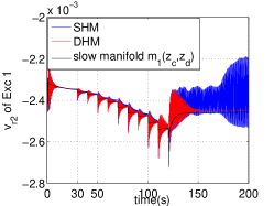
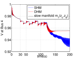
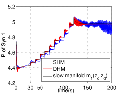
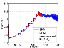
Figure 6: A comparison between the trajectory of the SHM and that of the DHM using the 14-bus system. The DHM fails to capture the instability of the SHM.

The failure of the DHM is caused by a violation of condition (iii), i.e., the condition of consistent attraction, in Theorem 2. When the discrete variables (i.e., the ratios of LTCs) change at 120s, the state of the DHM lies outside the stability region of the corresponding short-term stability model. To show this, the following simulations are conducted similar to the approach in [17]. When discrete variables jump at 110s, the trajectories of two fast variables of the corresponding short-term stability model starting from the state of the DHM are shown in Fig. 7. Observe that the trajectories converge to the SEP of the corresponding short-term stability model which shows that the condition of consistent attraction is satisfied at this time.

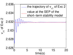
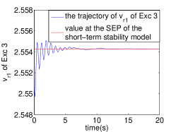
Figure 7: The trajectories of two fast variables in the short-term stability model when $\bm{z_{d}}$ change at 110s. The trajectory starting from the state of DHM converges to the SEP of the corresponding short-term stability model which shows that the condition of consistent attraction is satisfied.

But, if the discrete variables jump at 120s, the trajectories of the same two fast variables of the corresponding short-term stability model are shown in Fig. 8. Note that trajectories starting from the state of the DHM no longer converge to the SEP of the corresponding short-term stability model, and thus the state of the DHM lies outside the stability region of the short-term stability model. So, condition (iii) in Theorem 2 is violated, and the DHM can fail to provide a satisfactory approximation for the SHM, which is true in this case. Note that the condition of consistent attraction is a sufficient but unnecessary condition to ensure the stability of the DHM (Theorem 5-6 [17]). So, the DHM is stable in this case even though the condition of consistent contraction is violated.

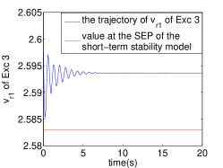
Figure 8: The trajectories of two fast variables in the short-term stability model when $\bm{z_{d}}$ change at 120s. The trajectory starting from the state of the DHM does not converge to the SEP of the corresponding short-term stability model. So, the condition of consistent attraction is violated.

From the viewpoint of physical mechanisms, the voltage collapse is caused by an insufficient power support when LTCs try to restore the load-side voltages in the long-term time scale. Immediately after the contingency, the system can maintain the short-term stability by the control of exciters. After that, LTCs start to work at 30s and try to restore the load-side voltages and then the corresponding load powers. At 112s, the OXL at GEN 1 is activated to protect the generator from overheating and thus restrict the power support from GEN 1. To make it even worse, the power output of DFIG at Bus 2 suddenly decreases as shown in Fig. 9 because of a sharp drop in the wind speed. The power imbalance between the loads and the generators finally leads to the voltage collapse in the SHM. In the DHM, however, the wind power does not change drastically as shown in Fig. 9, since the wind speed is supposed to be invariable. So, the DFIG at Bus 2 can provide enough power required by the action of LTCs to maintain the voltage stability of the DHM.

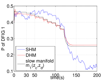
Figure 9: A comparison of the real power output of DFIG in the SHM and that in the DHM.

From this example, some important physical insights can be obtained. If the wind power plays a significant role in supporting power to maintain the stability, for example when the penetration level is high (8.42% in this example), then the stochastic properties of the wind may need to be considered in the stability analysis, especially when the system operates close to the stability boundary.

IV-B Numerical Example II

The second example using an IEEE 9-bus system is presented to reveal another cause for the failure of the DHM. In the system, the classical model of GEN is employed. A Weibull-distributed wind source drives a DFIG at Bus 3, and three GENs are equipped with TGs, AVRs, and OXLs, respectively, where the initial time delays of OXLs are 70s. In addition, three ERLs are located at Bus 5, 6, and 8, respectively; while three discrete LTCs are located at Bus 5-4, Bus 9-6, and Bus 2-7, respectively, the initial time delays of which are 60s and fixed tapping delays are 10s. At 1s, a fault occurs at Bus 6 and is cleared 5 cycles later. The parameter values are detailed in Appendix D.

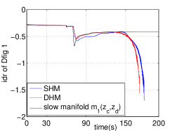
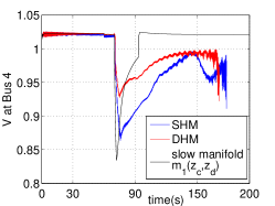
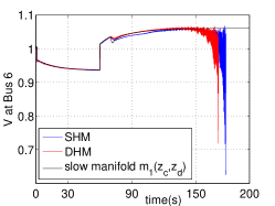
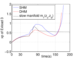
Figure 10: A comparisons between the trajectories of SHM and those of DHM. The results of Theorem 2 do not apply in this case as condition (i) is violated.

In this case, the slow manifold $\bm{m_{1}(\bm{z_{c}},\bm{z_{d}})}$ is unstable, which implies that nearby dynamics will move away from the slow manifold. As condition (i) in Theorem 1 and Theorem 2 is violated, neither the concentration of sample path stated in Theorem 1 nor the trajectory relationship described in Theorem 2 holds. The trajectory of the SHM is not concentrated around that of the DHM, i.e., the DHM cannot provide an accurate trajectory approximation for the SHM, but both of them are unstable in the long-term sense.

From the perspective of physical mechanisms, the instability is caused by the poor control of LTCs which are originally designed to help maintain the stability. The discrete switching of LTCs makes the slow manifold jump from the stable component of the constraint manifold to an unstable component such that the nearby trajectories move away. The switching events, such as LTCs and shunt compensation, are adopted commonly as countermeasures against the voltage instability. But, this example shows that great caution is necessary when executing those control strategies, because unexpected stability issues may arise, especially when more wind power is integrated into the power grid.

V Concluding Remarks

This paper proposes a comprehensive SDE-based framework for conducting the long-term stability analysis for the power grid with wind power generations. This framework incorporates the discrete dynamics induced by various control devices and the stochastic model of the wind speed with different probability distributions. To relieve the computational burden, a DHM is composed and can provide an accurate trajectory approximation and correct stability assessments for the SHM under some mild sufficient conditions. Numerical examples are further discussed to show that the DHM can fail in some critical cases because of a violation of the proposed sufficient conditions, which complements the proposed SDE-based framework and also highlights the necessity of the SHM in the stability analysis, especially if the system operates close to the stability boundary or experiences a high variability. For the future work, we plan to extend the present framework to the stability analysis of power grids with various other uncertainties and further improve the computational efficiency of the approximation methodology using the QSS model that integrates uncertainties.

Appendix A Proof of Theorem 1

Proof: Conditions (i) and (ii) ensure that all conditions of Theorem 1 [12] are satisfied for each fixed $\bm{z_{d}}(k)$, $k=0,1,...,N$. So, the conclusions of Theorem 1 [12] are valid for each continuous system of the SHM with fixed $\bm{z_{d}}(k)$. Then, there exist $\epsilon_{0}^{k}>0$, $h_{0}^{k}>0$, $\delta_{0}^{k}>0$, and a time $\tilde{\tau}_{k}$ of order $\epsilon|\mbox{log}h|$ such that whenever $\delta\leq\delta_{0}^{k}$, the following inequality

$$\mathbb{P}\{\exists\tau\in[\tilde{\tau}_{k},\tau_{k}):(\bm{z_{c}}^{k}(\tau),\bm{\bar{x}}^{k}(\tau),\bm{z_{d}}(k))\notin M(h)\}$$

$$\leq C_{n_{z_{c}},n_{x}}(\tau,\epsilon)e^{\frac{-h^{2}}{2\sigma^{2}}(1-O(h)-O(\epsilon))}$$ (26)

holds for all $\epsilon\leq\epsilon_{0}^{k}$, $h\leq h_{0}^{k}$, $k\in[0,1...N]$, on $[\tilde{\tau}_{k},\tau_{k+1})$ for $k\in[0,1,...N-1]$ or on $[\tilde{\tau}_{k},\infty]$ for $k=N$. Here, $(\bm{z_{c}}^{k}(\tau),\bm{\bar{x}}^{k}(\tau),\bm{z_{d}}(k))$ is the solution of each continuous system (17)-(18) of the SHM for fixed $\bm{z_{d}}(k)$ with initial condition $(\bm{z_{c}}^{k}(0),\bm{\bar{x}}^{k}(0),\bm{z_{d}}(k))$.

Let $\epsilon_{0}=\mbox{min}(\epsilon_{0}^{0},\epsilon_{0}^{1},...\epsilon_{0}^{N})$, $h_{0}=\mbox{min}(h_{0}^{0},h_{0}^{1},...h_{0}^{N})$, and $\delta_{0}=\mbox{min}(\delta_{0}^{0},\delta_{0}^{1},...\delta_{0}^{N})$. Then, for $\tau\in\Pi=\cup_{i=1}^{N-1}[\tilde{\tau}_{i},\tau_{i})\cup[\tilde{\tau}_{N},\infty]$, the following inequality

$$\mathbb{P}\{\exists\tau\in\Pi:~{}(\bm{z_{c}}(\tau),\bm{\bar{x}}(\tau),\bm{z_{d}})\notin M(h)\}$$

$$\leq C_{n_{z_{c}},n_{x}}(\tau,\epsilon)e^{\frac{-h^{2}}{2\sigma^{2}}(1-O(h)-O(\epsilon))}$$ (27)

holds for all $\epsilon\leq\epsilon_{0}$, $h\leq h_{0}$. This completes the proof.

Appendix B Proof of Theorem 2

Conditions (i)-(iii) ensure that all conditions of Theorem 2 [12] are satisfied for each fixed $\bm{z_{d}}(k)$, $k=0,1,...,N$. So, the conclusions of Theorem 2 [12] are valid for each continuous system of the SHM with fixed $\bm{z_{d}}(k)$. So, there exist $\epsilon_{0}^{k}>0$, $\delta_{0}^{k}>0$, a time $\tilde{\tau}_{k}$ of order $\epsilon|\mbox{log}h|$, and $\bar{\tau}_{k}$ such that whenever $\delta\leq\delta_{0}^{k}$ for all $\tau\in[\tilde{\tau}_{k},\bar{\tau}_{k}]$, the following estimates

$$|\bm{\bar{x}}^{k}(\tau)-\bm{\bar{x}_{D}}^{k}(\tau)| = O(\sigma),$$ (28)

$$|\bm{z_{c}}^{k}(\tau)-\bm{z_{cD}}^{k}(\tau)| = O(\sigma\sqrt{\epsilon}),$$ (29)

hold for all $\epsilon\in(0,\epsilon_{0}^{k})$, $0\leq k\leq N$, Here, $(\bm{z_{c}}^{k}(\tau),\bm{\bar{x}}^{k}(\tau),$ $\bm{z_{d}}(k))$ is the solution of each continuous system (17)-(18) of the SHM, and $(\bm{z_{cD}}^{k}(\tau),\bm{\bar{x}_{D}}^{k}(\tau),\bm{z_{d}}(k))$ is the solution of each continuous system (20)-(21) of the DHM for fixed $\bm{z_{d}}(k)$.

Let $\epsilon_{0}=\mbox{min}(\epsilon_{0}^{0},\epsilon_{0}^{1},\cdots,\epsilon_{0}^{N})$, $h_{0}=\mbox{min}(h_{0}^{0},h_{0}^{1},\cdots,h_{0}^{N})$, and $\delta_{0}=\mbox{min}(\delta_{0}^{0},\delta_{0}^{1},\cdots,\delta_{0}^{N})$. Similar to Theorem 1, one can show that for all $\tau\in\cup_{i=1}^{N}[\tilde{\tau}_{i},\bar{\tau}_{i}]$, the following estimates

$$|\bm{\bar{x}}(\tau)-\bm{\bar{x}_{D}}(\tau)| = O(\sigma)$$ (30)

$$|\bm{z_{c}}(\tau)-\bm{z_{cD}}(\tau)| = O(\sigma\sqrt{\epsilon})$$ (31)

hold for all $\epsilon\in(0,\epsilon_{0})$. The proof of the theorem is completed.

Appendix C Parameter Values of Numerical Example I

The system is modified from the 14-bus test case in PSAT-2.1.6. The GEN at Bus 2 is replaced by DFIG. The parameter values are given in Table I-V.

TABLE I: Doubly-fed induction generator parameter values

Parameter	Value
stator resistance $r_{s}$	$0.01$p.u.
stator reactance $x_{s}$	$0.1$p.u.
rotor resistance $r_{r}$	$0.01$p.u.
rotor reactance $x_{r}$	$0.08$p.u.
magnetizing reactance $x_{\mu}$	$3$p.u.
rotor inertia $H_{m}$	$3$KWs/KVA
pitch control gain $K_{p}$	$10$
pitch control time constant $T_{p}$	$3$s
voltage control gain $K_{v}$	10
power control time constant $T_{\epsilon}$	$0.01$s
rotor radius $R$	$75$m
number of poles $n_{p}$	$4$
number of blades $n_{b}$	$3$
gear box ratio $\eta_{GB}$	$0.0112$
maximum active power $p^{max}$	$2$p.u.
minimum active power $p^{min}$	$-1$p.u.
maximum reactive power $q^{max}$	$2$p.u.
minimum reactive power $q^{min}$	$-1$p.u.
number of machines $n_{g}$	$1$

TABLE II: Turbine governor parameter values

Parameter	Value
reference speed $\omega^{0}_{ref}$	$1$p.u.
droop $R$	$0.02$p.u.
maximum turbine output $p^{max}$	$1.2$p.u.
minimum turbine output $p^{min}$	$0$p.u.
governor time constant $T_{s}$	$0.1$s
servo time constant $T_{c}$	$0.45$s
transient gain time constant $T_{3}$	$0$s
power fraction time constant $T_{4}$	$12$s
reheat time constant $T_{5}$	$50$s

TABLE III: Load tap changer parameter values for the ones at bus 4-9, bus 12-13 and bus 2-4

Parameter	Value
the reference voltage $v_{0}$	$1.005$, $1.01$, $0.995$
half of the deadband $d$	$0.005$, $0.1$, $0.025$ p.u.
tap step $r$	$0.025$
upper tap limit $r^{max}$	$1.2$
lower tap limit $r^{min}$	$0.7$
the initial time delay $\triangle{T_{0}}$	$30$s
the sequential time delay $\triangle{T_{k}}$	$10$s

TABLE IV: Exponential recovery load parameter values

Parameter	Value
active power percentage $k_{p}$	$100\%$
reactive power percentage $k_{q}$	$100\%$
active power time constant $T_{p}$	$10$s
reactive power time constant $T_{q}$	$10$s
static active power exponent $\alpha_{s}$	$1$
dynamic active power exponent $\alpha_{t}$	$1.5$ for the load at Bus 9
	$5$ for the others
static reactive power exponent $\beta_{s}$	$2$
dynamic reactive power exponent $\beta_{t}$	$2.5$ for the load at Bus 9
	$10$ for the others

TABLE V: Over excitation limiter parameter values

Parameter	Value
maximum field current $i_{f}^{lim}$	$5.1$p.u.
integrator time constant $T_{0}$	$12$s
maximum output signal $v_{\mbox{oxl}}$	$100$p.u.

Appendix D Parameter Values of Numerical Example II

The system is modified from the 9-bus test system in PSAT-2.1.6. There is a DIFG at Bus 3. The parameters of the DFIG are the same as those for Numerical Example I in Table I. The parameters of other devices are shown in Table VI-IX.

TABLE VI: Turbine governor parameter values

Parameter	Value
reference speed $\omega^{0}_{ref}$	$1$p.u.
droop $R$	$0.02$p.u.
maximum turbine output $p^{max}$	$2$p.u.
minimum turbine output $p^{min}$	$0.3$p.u.
governor time constant $T_{s}$	$0.1$s
servo time constant $T_{c}$	$0.45$s
transient gain time constant $T_{3}$	$0$s
power fraction time constant $T_{4}$	$12$s
reheat time constant $T_{5}$	$50$s

TABLE VII: Exponential recovery load parameter values

Parameter	Value
active power percentage $k_{p}$	$40\%$
reactive power percentage $k_{q}$	$40\%$
active power time constant $T_{p}$	$10$s
reactive power time constant $T_{q}$	$10$s
static active power exponent $\alpha_{s}$	$1$
dynamic active power exponent $\alpha_{t}$	$10$ for the load at Bus 4
	$5$ for the others
static reactive power exponent $\beta_{s}$	$2$
dynamic reactive power exponent $\beta_{t}$	$20$ for the load at Bus 4
	$10$ for the others

TABLE VIII: Load tap changer parameter values for the ones at bus 5-4, bus 9-6, and bus 2-7

Parameter	Value
the reference voltage $v_{0}$	$1.005$, $1.005$, $1.02$
half of the deadband $d$	$0.025$, $0.025$, $0.04$ p.u.
tap step $r$	$0.12$
upper tap limit $r^{max}$	$1.1$
lower tap limit $r^{min}$	$0.9$
the initial time delay $\triangle{T_{0}}$	$60$s
the sequential time delay $\triangle{T_{k}}$	$10$s

TABLE IX: Over excitation limiter parameter values

Parameter	Value
maximum field current $i_{f}^{lim}$	$2.02$, $1.3$, $1.32$p.u.
integrator time constant $T_{0}$	$10$s for GEN 1-2
	$30$s for GEN 3
maximum output signal $v_{\mbox{oxl}}$	$100$p.u.

Xiaozhe Wang (S’13-M’15) is currently an Assistant Professor in the department of Electrical and Computer Engineering at McGill University. She received the Ph.D. degree and the M. Eng in the School of Electrical and Computer Engineering from Cornell University, Ithaca, NY, USA, in 2015 and 2011, respectively, and the B.S. degree in Information Science & Electronic Engineering from Zhejiang University, Zhejiang, China, in 2010. She was a Research Aid Intern at Argonne National Laboratory, Argonne, IL, USA, in 2014.

Tao Wang (M’13) received the B.S. degree in mathematics from the University of Science and Technology of China, Anhui, China in 2006, and the Ph.D. degree in mathematics from the Pennsylvania State University, University Park, PA 16802, USA in 2011. Since 2012, he has been a visiting scientist at the School of Electrical and Computer Engineering, Cornell University, Ithaca, NY 14853, USA. His research interests include nonlinear systems and control, mathematical programming, geometric analysis, and applications in electrical engineering and management of invasive disasters.

Hsiao-Dong Chiang (M’87-SM’91-F’97) received the Ph.D. degree in EECS from the University of California at Berkeley in 1986. He is Professor of Electrical Engineering at Cornell University, Ithaca, New York. He and his research team have published more than 350 papers in refereed journals and conference proceedings. His current research interests include nonlinear system theory, nonlinear computation, nonlinear optimization and their practical applications. He was an associate editor IEEE Transactions on Circuits and Systems (1990-91, 1993-1995). He holds 17 U.S. and oversea patents and several consultant positions. He is Author of the book “Direct Methods for Power System Stability Analysis: Theoretical Foundation, BCU Methodology and Applications”, John Wiley & Sons, 2011 and of the book “Stability region of nonlinear dynamical system: theory, optimal estimation and applications”, Cambridge Press, 2015.

Jianhui Wang (M’07-SM’12 received the Ph.D. degree in electrical engineering from Illinois Institute of Technology, Chicago, IL, USA, in 2007. Presently, he is the Section Lead for Advanced Power Grid Modeling at the Energy Systems Division at Argonne National Laboratory, Argonne, IL, USA. Dr. Wang is the secretary of the IEEE Power & Energy Society (PES) Power System Operations, Planning & Economics Committee. He is an associate editor of Journal of Energy Engineering and an editorial board member of Applied Energy. He is also an affiliate professor at Auburn University and an adjunct professor at University of Notre Dame. He has held visiting positions in Europe, Australia and Hong Kong including a VELUX Visiting Professorship at the Technical University of Denmark (DTU). Dr. Wang is the Editor-in-Chief of the IEEE Transactions on Smart Grid and an IEEE PES Distinguished Lecturer. He is also the recipient of the IEEE PES Power System Operation Committee Prize Paper Award in 2015.

Hui Liu (M’12) was born in Sichuan, China. He received the M. S. and Ph.D. degrees from the college of electrical engineering, Guangxi University, China, both in Electrical Engineering. He worked in Tsinghua University as a postdoctoral fellow from 2011 to 2013. He is an associate professor of school of electrical and information engineering, Jiangsu University, China. His research interests include power system control and electric vehicles.

References

- [1] D. Gautam, V. Vittal, and T. Harbour, “Impact of increased penetration of DFIG-based wind turbine generators on transient and small signal stability of power systems,” IEEE Trans. Power Syst., vol 24, no. 3, pp. 1426-1434, 2009.
- [2] P. Ledesma, J. Usaola, and J. L. Rodriguez, “Transient stability of a fixed speed wind farm,” Renewable Energy, vol. 28, no. 9, pp. 1341-1355, 2003.
- [3] L. Meegahapola, D. Flynn, “Impact on transient and frequency stability for a power system at very high wind penetration,” IEEE PES General Meeting, 2010.
- [4] A. Kanchanaharuthai, V. Chankong, and K. Loparo, “Transient stability and voltage regulation in power systems with renewable distributed energy resources,” IEEE Energytech, May 2011.
- [5] J. G. Slootweg, W. L. Kling, “Impacts of distributed generation on power system transient stability,” IEEE PES Summer Meeting, 2002.
- [6] E. Vittal, M. O’Malley, and A. Keane, “Rotor angle stability with high penetrations of wind generation,” IEEE Trans. Power Syst., vol. 27, no. 1, pp. 353-362, 2012.
- [7] R. R. Londero, C. M. Affonso, and J. P. A. Vieira, “Long-term voltage stability analysis of variable speed wind generators,” IEEE Trans. Power Syst., vol. 30, no. 1, pp. 439-447, Jan. 2015.
- [8] R. R. Londero, C. M. Affonso, J. P. A. Vieira, and U. H. Bezerra, “Impact of different DFIG wind turbines control modes on long-term voltage stability,” IEEE PES-ISGT Europe, Berlin, 2012.
- [9] T. Odun-Ayo, M. L. Crow, “Structure-preserved power system transient stability using stochastic energy functions,” IEEE Trans. Power Syst., vol. 27, no. 3, pp. 1450-1458.
- [10] B. Yuan, M. Zhou, G. Li, and X. P. Zhang, “Stochastic small-signal stability of power systems with wind power generation,” IEEE Trans. Power Syst., doi: 10.1109/TPWRS.2014.2353014.
- [11] H. Mohammed, C. O. Nwankpa, “Stochastic analysis and simulation of grid-connected wind energy conversion system,” IEEE Trans. Energy Conver., vol. 15, no. 1, pp. 85-90, 2000.
- [12] X. Wang, H. D. Chiang, J. Wang, H. Liu, T. Wang, “Long-term stability analysis of power systems with wind power based on stochastic differential equations: model development and foundations,” IEEE Trans. Sustain. Energy, vol. 6, no. 4, pp. 1534-1542, October 2015.
- [13] T. V. Cutsem, C. Vournas, Voltage Stability of Electric Power Systems. Boston/London/Dordrecht: Kluwer Academic Publishers, 1998.
- [14] T. V. Cutsem, “Voltage instability: phenomena, countermeasures, and analysis methods,” Proc. IEEE, vol 88, no. 2 pp. 208-227, 2000.
- [15] P. Kundur, Power System Stability and Control. New York: McGraw-Hill, Inc. 1994.
- [16] F. Milano, “ Hybrid control model of under load tap changers,” IEEE Trans. Power Del., vol. 26, no. 4, pp. 2837-2844, Oct. 2011.
- [17] X. Wang, H. D. Chiang, “Analytical studies of quasi steady-state model in power system long-term stability analysis,” IEEE Trans. Circuits Syst. I, vol. 61, no. 3, pp. 943-956, 2014.
- [18] R. Zárate-Miñano, M. Anghel, and F. Milano, “Continuous wind speed models based on stochastic differential equations,” Applied Energy, vol. 104, pp. 42-49, 2013.
- [19] H. D. Chiang, Direct Methods for Stability Analysis of Electric Power Systems-Theoretical Foundation, BCU Methodologies, and Applications. New Jersey: John Wiley & Sons, Inc, 2011.
- [20] N. Berglund, B. Gentz, Noise-induced phenomena in slow-fast dynamical systems: a sample-paths approach, Springer, 2006.
- [21] N. Berglund, B. Gentz, “Geometric singular perturbation theory for stochastic differential equations,” J. Differ. Equations, vol. 191, no. 1, pp. 1-54, 2003.
- [22] M. I. Freidlin, J. Szcs, A. D. Wentzell, Random Perturbations of Dynamical Systems. New York: 2nd Edition, Springer, 1998.
- [23] X. Wang, H. D. Chiang, “Numerical investigations on quasi steady-state model for voltage stability: limitations and nonlinear analysis,” Int. Trans. Electr. Energy Syst., vol. 24, no. 11, pp. 1586-1599, 2014.
- [24] H. Khalil, Nonlinear System, 3rd ed, New York: Macmillan Publishing Company, 2002.
- [25] Luis F. C. Alberto, H. D. Chiang, “Theoretical foundation of CUEP method for two-time scale power system models,” IEEE PES General Meeting, 2009.
- [26] R. Christie, “Power Systems Test Case Archive,” Electrical Engineering dept., University of Washington, Apr. 2000. [Online]. Available: http://www.ee.washington.edu/research/pstca.
- [27] F. Milano, “An open source power system analysis toolbox,” IEEE Trans. Power Syst., vol. 20, no. 3, pp. 1199-1206, 2005.
- [28] F. Milano, Documentation for PSAT version 2.1.5, November 01, 2009. Available: http://faraday1.ucd.ie/psat.html.