1920173143181
Self-Stabilizing Disconnected Components Detection and Rooted Shortest-Path Tree Maintenance in Polynomial Steps††thanks: This study has been partially supported by the anr projects Descartes (ANR-16-CE40-0023), Estate (ANR-16-CE25-0009), and Macaron (ANR-13-JS02-002). This study has been carried out in the frame of “the Investments for the future” Programme IdEx Bordeaux – cpu (ANR-10-IDEX-03-02). A preliminary version of this paper appeared in the Proceedings of the 20th International Conference on Principles of Distributed Systems (OPODIS 2016) [DIJ16].
Abstract
We deal with the problem of maintaining a shortest-path tree rooted at some process in a network that may be disconnected after topological changes. The goal is then to maintain a shortest-path tree rooted at in its connected component, , and make all processes of other components detecting that is not part of their connected component. We propose, in the composite atomicity model, a silent self-stabilizing algorithm for this problem working in semi-anonymous networks, where edges have strictly positive weights. This algorithm does not require any a priori knowledge about global parameters of the network. We prove its correctness assuming the distributed unfair daemon, the most general daemon. Its stabilization time in rounds is at most , where is the maximum number of non-root processes in a connected component and is the hop-diameter of . Furthermore, if we additionally assume that edge weights are positive integers, then it stabilizes in a polynomial number of steps: namely, we exhibit a bound in , where is the maximum weight of an edge and is the number of processes.
keywords:
distributed algorithm, self-stabilization, routing algorithm, shortest path, disconnected network, shortest-path tree1 Introduction
Given a connected undirected edge-weighted graph , a shortest-path (spanning) tree rooted at node is a spanning tree of , such that for every node , the unique path from to in is a shortest path from to in . This data structure finds applications in the networking area (n.b., in this context, nodes actually represent processes), since many distance-vector routing protocols, like RIP (Routing Information Protocol) and BGP (Border Gateway Protocol), are based on the construction of shortest-path trees. Indeed, such algorithms implicitly builds a shortest-path tree rooted at each destination.
From time to time, the network may be split into several connected components due to the network dynamics. In this case, routing to process correctly operates only for the processes of its connected component, . Consequently, in other connected components, information to reach should be removed to gain space in routing tables, and to discard messages destined to (which are unable to reach anyway) and thus save bandwidth. The goal is then to make the network converging to a configuration where every process of knows a shortest path to and every other process detects that is not in its own connected component. We call this problem the Disconnected Components Detection and rooted Shortest-Path tree Maintenance (DCDSPM) problem. Notice that a solution to this problem allows to prevent the well-known count-to-infinity problem [LGW04], where the distances to some unreachable process keep growing in routing tables because no process is able to detect the issue.
When topological changes are infrequent, they can be considered as transient faults [Tel01] and self-stabilization [Dij74] — a versatile technique to withstand any finite number of transient faults in a distributed system — becomes an attractive approach. A self-stabilizing algorithm is able to recover without external (e.g., human) intervention a correct behavior in finite time, regardless of the arbitrary initial configuration of the system, and therefore, also after the occurrence of transient faults, provided that these faults do not alter the code of the processes.
A particular class of self-stabilizing algorithms is that of silent algorithms. A self-stabilizing algorithm is silent [DGS99] if it converges to a global state where the values of communication registers used by the algorithm remain fixed. Silent (self-stabilizing) algorithms are usually proposed to build distributed data structures, and so are well-suited for the problem considered here. As quoted in [DGS99], the silent property usually implies more simplicity in the algorithm design, moreover a silent algorithm may utilize less communication operations and communication bandwidth.
For the sake of simplicity, we consider here a single destination process , called the root. However, the solution we will propose can be generalized to work with any number of destinations, provided that destinations can be distinguished. In this context, we do not require the network to be fully identified. Rather, should be distinguished among other processes, and all non-root processes are supposed to be identical: we consider semi-anonymous networks.
In this paper, we propose a silent self-stabilizing algorithm, called Algorithm , for the DCDSPM problem with a single destination process in semi-anonymous networks. Algorithm does not require any a priori knowledge of processes about global parameters of the network, such as its size or its diameter. Algorithm is written in the locally shared memory model with composite atomicity introduced by Dijkstra [Dij74], which is the most commonly used model in self-stabilization. In this model, executions proceed in (atomic) steps, and a self-stabilizing algorithm is silent if and only if all its executions are finite. Moreover, the asynchrony of the system is captured by the notion of daemon. The weakest (i.e., the most general) daemon is the distributed unfair daemon. Hence, solutions stabilizing under such an assumption are highly desirable, because they work under any other daemon assumption. Interestingly, self-stabilizing algorithms designed under this assumption are easier to compose (composition techniques are widely used to design and prove complex self-stabilizing algorithms). Moreover, time complexity (the stabilization time, mainly) can be bounded in terms of steps only if the algorithm works under an unfair daemon. Otherwise (e.g., under a weakly fair daemon), time complexity can only be evaluated in terms of rounds, which capture the execution time according to the slowest process. There are many self-stabilizing algorithms proven under the distributed unfair daemon, e.g., [ACD+17, CDD+15, DLV11a, DLV11b, GHIJ14]. However, analyses of the stabilization time in steps is rather unusual and this may be an important issue. Indeed, this complexity captures the amount of computations an algorithm needs to recover a correct behavior. Now, recently, several self-stabilizing algorithms, which work under a distributed unfair daemon, have been shown to have an exponential stabilization time in steps in the worst case. In [ACD+17], silent leader election algorithms from [DLV11a, DLV11b] are shown to be exponential in steps in the worst case. In [DJ16], the Breadth-First Search (BFS) algorithm of Huang and Chen [HC92] is also shown to be exponential in steps. Finally, in [Ga16] authors show that the first silent self-stabilizing algorithm for the DCDSPM problem (still assuming a single destination) they proposed in [GHIJ14] is also exponential in steps.
1.1 Contribution
Algorithm proposed here is proven assuming the distributed unfair daemon. We also study its stabilization time in rounds. We establish a bound of at most rounds, where is the maximum number of non-root processes in a connected component and is the hop-diameter of (defined as the maximum over all pairs of nodes in of the minimum number of edges in a shortest path from to ).
Furthermore, is the first silent self-stabilizing algorithm for the DCDSPM problem which, assuming that the edge weights are positive integers, achieves a polynomial stabilization time in steps. Namely, in this case, the stabilization time of is at most , where is the maximum weight of an edge and is the number of processes. (N.b., this stabilization time is less than or equal to , for all .)
Finally, notice that when all weights are equal to one, the DCDSPM problem reduces to a BFS tree maintenance and the step complexity becomes at most , which is less than or equal to for all .
1.2 Related Work
To the best of our knowledge, only one self-stabilizing algorithm for the DCDSPM problem has been previously proposed in the literature [GHIJ14]. This algorithm is silent and works under the distributed unfair daemon, but, as previously mentioned, it is exponential in steps. However, it has a slightly better stabilization time in rounds, precisely at most rounds111In fact, [GHIJ14] announced rounds, but it is easy to see that this complexity can be reduced to ..
There are several shortest-path spanning tree algorithms in the literature that do not consider the problem of disconnected components detection. The oldest distributed algorithms are inspired by the Bellman-Ford algorithm [Bel58, FJ56]. Self-stabilizing shortest-path spanning tree algorithms have then been proposed in [CS94, HL02], but these two algorithms are proven assuming a central daemon, which only allows sequential executions. However, in [Hua05b], Tetz Huang proves that these algorithms actually work assuming the distributed unfair daemon. Nevertheless, no upper bounds on the stabilization time (in rounds or steps) are given. More recently, Cobb and Huang [CH09] proposed an algorithm constructing shortest-path trees based on any maximizable routing metrics. This algorithm does not require a priori knowledge about the network but it is proven only for the central weakly-fair daemon. It runs in a linear number of rounds and no analysis is given on the number of steps.
Self-stabilizing shortest-path spanning tree algorithms are also given in [AGH90, CG02, JT03]. These algorithms additionally ensure the loop-free property in the sense that they guarantee that a spanning tree structure is always preserved while edge costs change dynamically. However, none of these papers consider the unfair daemon, and consequently their step complexity cannot be analyzed.
Whenever all edges have weight one, shortest-path trees correspond to BFS trees. In [DDL12], the authors introduce the disjunction problem as follows. Each process has a constant input bit, 0 or 1. Then, the problem consists for each process in computing an output value equal to the disjunction of all input bits in the network. Moreover, each process with input bit 1 (if any) should be the root of a tree, and each other process should join the tree of the closest input bit 1 process, if any. If there is no process with input bit 1, the execution should terminate and all processes should output 0. The proposed algorithm is silent and self-stabilizing. Hence, if we set the input of a process to 1 if and only if it is the root, then their algorithm solves the DCDSPM problem when all edge-weights are equal to one, since any process which is not in will compute an output 0, instead of 1 for the processes in . The authors show that their algorithm stabilizes in rounds, but no step complexity analysis is given. Now, as their approach is similar to [DLV11b], it is not difficult to see that their algorithm is also exponential in steps.
Several other self-stabilizing BFS tree algorithms have been proposed, but without considering the problem of disconnected components detection. Chen et al. present the first self-stabilizing BFS tree construction in [CYH91] under the central daemon. Huang and Chen present the first self-stabilizing BFS tree construction in [HC92] under the distributed unfair daemon, but recall that this algorithm has been proven to be exponential in steps in [DJ16]. Finally, notice that these two latter algorithms [CYH91, HC92] require that the processes know the exact number of processes in the network.
According to our knowledge, only the following works [CDV09, CRV11] take interest in the computation of the number of steps required by their BFS algorithms. The algorithm in [CDV09] is not silent and has a stabilization time in steps, where is the maximum degree in the network. The silent algorithm given in [CRV11] has a stabilization time rounds and steps.
Silent self-stabilizing algorithms that construct spanning trees of arbitrary topologies are given in [Cou09, KK05]. The solution proposed in [Cou09] stabilizes in at most rounds and steps, while the algorithm given in [KK05] stabilizes in steps (its round complexity is not analyzed).
Several other papers propose self-stabilizing algorithms stabilizing in both a polynomial number of rounds and a polynomial number of steps, e.g., [ACD+17] (for the leader election), [CDPV06, CDV05] (for the DFS token circulation). The silent leader election algorithm proposed in [ACD+17] stabilizes in at most rounds and steps. DFS token circulations given in [CDPV06, CDV05] execute each wave in rounds and steps using space per process for the former, and rounds and steps using space per process for the latter.
1.3 Roadmap
In the next section, we present the computational model and basic definitions. In Section 3, we describe Algorithm . Its proof of correctness and a complexity analysis in steps are given in Section 4, whereas an analysis of the stabilization time in rounds is proposed in Section 5. Finally, we make concluding remarks in Section 6.
2 Preliminaries
We consider distributed systems made of interconnected processes. Each process can directly communicate with a subset of other processes, called its neighbors. Communication is assumed to be bidirectional. Hence, the topology of the system can be represented as a simple undirected graph , where is the set of processes and the set of edges, representing communication links. Every process can distinguish its neighbors using a local labeling of a given datatype . All labels of ’s neighbors are stored into the set . Moreover, we assume that each process can identify its local label in the set of each neighbor . Such labeling is called indirect naming in the literature [SK87]. By an abuse of notation, we use to designate both the process itself, and its local labels.
Each edge has a strictly positive weight, denoted by . This notion naturally extends to paths: the weight of a path in is the sum of its edge weights. The weighted distance between the processes and , denoted by , is the minimum weight of a path from to . Of course, if and only if and belong to two distinct connected components of .
We use the composite atomicity model of computation [Dij74, Dol00] in which the processes communicate using a finite number of locally shared registers, called variables. Each process can read its own variables and those of its neighbors, but can write only to its own variables. The state of a process is defined by the values of its local variables. A configuration of the system is a vector consisting of the states of every process.
A distributed algorithm consists of one local program per process. We consider semi-uniform algorithms, meaning that all processes except one, the root , execute the same program. In the following, for every process , we denote by the set of processes (including ) in the same connected component of as . In the following is simply referred to as the connected component of . We denote by the maximum number of non-root processes in a connected component of . By definition, .
The program of each process consists of a finite set of rules of the form . Labels are only used to identify rules in the reasoning. A guard is a Boolean predicate involving the state of the process and that of its neighbors. The action part of a rule updates the state of the process. A rule can be executed only if its guard evaluates to true; in this case, the rule is said to be enabled. A process is said to be enabled if at least one of its rules is enabled. We denote by the subset of processes that are enabled in configuration .
When the configuration is and , a non-empty set is selected; then every process of atomically executes one of its enabled rules, leading to a new configuration , and so on. The transition from to is called a step. The possible steps induce a binary relation over , denoted by . An execution is a maximal sequence of configurations such that for all . The term “maximal” means that the execution is either infinite, or ends at a terminal configuration in which no rule is enabled at any process.
Each step from a configuration to another is driven by a daemon. We define a daemon as a predicate over executions. We said that an execution is an execution under the daemon , if holds. In this paper we assume that the daemon is distributed and unfair. “Distributed” means that while the configuration is not terminal, the daemon should select at least one enabled process, maybe more. “Unfair” means that there is no fairness constraint, i.e., the daemon might never select an enabled process unless it is the only enabled process. In other words, the distributed unfair daemon corresponds to the predicate , i.e., this is the most general daemon.
In the composite atomicity model, an algorithm is silent if all its possible executions are finite. Hence, we can define silent self-stabilization as follows.
Definition 1 (Silent Self-Stabilization).
Let be a non-empty subset of configurations, called set of legitimate configurations. A distributed system is silent and self-stabilizing under the daemon for if and only if the following two conditions hold:
-
•
all executions under are finite, and
-
•
all terminal configurations belong to .
We use the notion of round [DIM93] to measure the time complexity. The definition of round uses the concept of neutralization: a process is neutralized during a step , if is enabled in but not in configuration . Then, the rounds are inductively defined as follows. The first round of an execution is the minimal prefix , such that every process that is enabled in either executes a rule or is neutralized during a step of . Let be the suffix of . The second round of is the first round of , and so on.
The stabilization time of a silent self-stabilizing algorithm is the maximum time (in steps or rounds) over every execution possible under the considered daemon (starting from any initial configuration) to reach a terminal (legitimate) configuration.
3 Algorithm
This section is devoted to the presentation of our algorithm, Algorithm (which stands for Rooted Shortest-Path). The code of Algorithm is given in Algorithm 1.
| : | ; | |
| ; | ||
| : | ||||
|---|---|---|---|---|
| : | ||||
| ( ) | ||||
| : | ||||
| : | ||||
| : |
3.1 Variables
In , each process maintains three variables: , , and . Those three variables are constant for the root process222We should emphasize that the use of constants at the root is not a limitation, rather it allows to simplify the design and proof of the algorithm. Indeed, these constants can be removed by adding a rule to correct all root’s variables, if necessary, within a single step., : , 333 is a particular value which is different from any value in ., and . For each non-root process , we have:
-
•
, this variable gives the status of the process. , , , and respectively stand for Isolated, Correct, Error Broadcast, and Error Feedback. The two first states, and , are involved in the normal behavior of the algorithm, while the two last ones, and , are used during the correction mechanism. Precisely, (resp. means that believes it is in (resp. not in ). The meaning of status and will be further detailed in Subsection 3.3.
-
•
, a parent pointer. If , should designate a neighbor of , referred to as its parent, and in a terminal configuration, the parent pointers exhibit a shortest path from to .
Otherwise (), the variable is meaningless.
-
•
, the distance value. If , then in a terminal configuration, gives the weight of the shortest path from to .
Otherwise (), the variable is meaningless.
3.2 Normal Execution
Consider any configuration, where every process satisfies , and refer to such a configuration as a normal initial configuration. Each configuration reachable from a normal initial configuration is called a normal configuration, otherwise it is an abnormal configuration. Recall that in all configurations. Then, starting from a normal initial configuration, all processes in a connected component different from are disabled forever. Focus now on the connected component . Each neighbor of is enabled to execute . A process eventually chooses as parent by executing this rule, which in particular sets its status to . Then, executions of rule are asynchronously propagated in until all its processes have status : when a process with status finds one of its neighbor with status it executes , i.e. takes status and chooses as parent its neighbor with status such that is minimum, being updated accordingly. In parallel, rules are executed to reduce the weight of the tree rooted at : when a process with status can reduce by selecting another neighbor with status as parent, it chooses the one allowing to minimize by executing . Hence, eventually, the system reaches a terminal configuration, where the tree rooted at is a shortest-path tree spanning all processes of .
3.3 Error Correction
Assume now that the system is in an abnormal configuration. Thanks to the predicate , some non-root processes locally detect that their state is inconsistent with that of their neighbors. We call abnormal roots such processes. Informally (see Algorithm for the formal definition), a process is an abnormal root if is not isolated (i.e., ) and satisfies one of the following four conditions:
-
1.
its parent pointer does not designate a neighbor,
-
2.
its parent has status ,
-
3.
its distance value is inconsistent with the distance value of its parent, or
-
4.
its status is inconsistent with the status of its parent.
Every non-root process that is not an abnormal root satisfies one of the two following cases. Either is isolated, i.e., , or points to some neighbor (i.e., ) and the state of is coherent w.r.t. the state of its parent. In this latter case, , i.e., is a “real” child of its parent (see Algorithm for the formal definition). Consider a path (with ) such that is either or an abnormal root, and . is acyclic and called a branch rooted at . Hence, we define the normal tree (resp. an abnormal tree , for any abnormal root ) as the set of all processes that belong to a branch rooted at (resp. ).
Then, the goal is to remove all abnormal trees so that the system recovers a normal configuration. For each abnormal tree , we have two cases. In the former case, the abnormal root of can join another tree using rule , making a subtree of . In the latter case, is entirely removed in a top-down manner starting from its (abnormal) root . Now, in that case, we have to prevent the following situation: leaves ; this removal creates some trees, each of those is rooted at a previous child of ; and later joins one of those (created) trees. Hence, the idea is to freeze , before removing it. By freezing we mean assigning each member of the tree to a particular state, here , so that (1) no member of the tree is allowed to execute , and (2) no process can join the tree by executing . Once frozen, the tree can be safely deleted from its root to its leaves.
The freezing mechanism (inspired from [BCV03]) is achieved using the status and , and the rules and . If a process is not involved into any freezing operation, then its status is or . Otherwise, it has status or and no neighbor can select it as its parent. These two latter states are actually used to perform a “Propagation of Information with Feedback” [Cha82, Seg83] in the abnormal trees. This is why status means “Error Broadcast” and means “Error Feedback”. From an abnormal root, the status is broadcast down in the tree using rule . Then, once the wave reaches a leaf, the leaf initiates a convergecast -wave using rule . Once the -wave reaches the abnormal root, the tree is said to be dead, meaning that all processes in the tree have status and, consequently, no other process can join it. So, the tree can be safely deleted from its abnormal root toward its leaves. There is two possibilities for the deletion. If the process to be deleted has a neighbor with status , then it executes rule to directly join another “alive” tree. Otherwise, becomes isolated by executing rule , and may join another tree later.
Let be a process belonging to an abnormal tree of which it is not the root. Let be its parent. From the previous explanation, it follows that during the correction, until resets by or . Now, due to the arbitrary initialization, the status of and may not be coherent, in this case should also be an abnormal root. Precisely, as formally defined in Algorithm 1, the status of is incoherent w.r.t the status of its parent if and .
3.4 Example
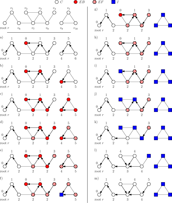
An example of synchronous execution of is given in Figure 1. We consider the network topology given on the top left of the figure. The names are only given to ease the explanation (recall that we consider semi-anonymous networks where only the root is distinguished). The network contains eleven processes divided into two connected components. Let be a process. In the synchronous execution described from configuration a) to configuration m), the color of indicates its status , according to the legend on the top of the figure. The number next to gives its distance value, . If there is an arrow outgoing from , this arrow designates the neighbor of pointed as parent, i.e., . Otherwise, this means that .
In the initial configuration a), there are two abnormal roots: and , indeed and . The status of is already equal to and this value should be broadcast down in its subtree. In contrast, has status and, consequently, should initiate the broadcast of . Note also that can reduce its distance value by modifying its parent pointer. Hence, in the step a) b), takes status (rule ), selects as parent (rule ), and finally the unique child of takes status (rule ).
In the step b) c), is propagated down the two abnormal trees: , , , and execute . In configuration c), the value has reached three leaves: , , and . These processes are then enabled to initiate a convergecast -wave. Hence, in the step c) d), , , and execute , while the last leaf takes status ().
In configuration d), all children of have status , so is enabled to take status too (). In contrast, should wait until its child takes status . Hence, in the step d) e), takes status (), its abnormal tree becomes frozen, while the last leaf of the second abnormal tree initiates a convergecast -wave (rule ).
In the step e) f), leaves its tree and becomes isolated by rule , while takes status by . Since all its children have now status , can take status by in step f) g), while and become isolated by rule in the same step. Remark then that in g), all processes in the connected component are isolated and, since is not part of this component, they are disabled forever. In the step g) h), the abnormal root of the remaining abnormal tree takes status (). So, the abnormal tree rooted at is frozen in configuration h). In the step h) i), leaves its tree and becomes isolated by rule . Then, becomes isolated in step i) j) (rule ). In step j) k), becomes isolated (rule ), while joins the normal tree (the tree rooted at ) by rule . In the last two steps, , , , and then successively join the normal tree by rule , and configuration m) is terminal.
4 Correctness and Step Complexity of Algorithm
4.1 Definitions
Before proceeding with the proof of correctness and the step complexity analysis, we define some useful concepts.
Definition 2 (Abnormal Root).
Every process that satisfies is said to be an abnormal root.
Definition 3 (Alive Abnormal Root).
A process is said to be an alive abnormal root (resp. a dead abnormal root) if is an abnormal root and has a status different from (resp. has status ).
Definition 4 (Branch).
A branch is a sequence of processes for some integer , such that is or an abnormal root and, for every , we have . The process is said to be at depth and is called a sub-branch. If , the branch is said to be illegal, otherwise, the branch is said to be legal.
Observation 1.
A branch depth is at most . A process having status does not belong to any branch. If a process has status (resp. ), then all processes of a sub-branch starting at have status (resp. ).
Definition 5 (Legitimate State).
A process is said to be in a legitimate state if satisfies one of the following three conditions:
-
1.
,
-
2.
, , , , and , or
-
3.
and .
Observation 2.
Every process such that and is enabled.
Definition 6 (Legitimate Configuration).
A legitimate configuration is any configuration where every process is in a legitimate state. We denote by the set of all legitimate configurations of Algorithm .
Let be a configuration. Let be the subgraph, where . By Definition 5 (point 2), we deduce the following observation.
Observation 3.
In every legitimate configuration , is a shortest-path tree spanning all processes of .
4.2 Partial Correctness
We now prove that the set of terminal configurations is exactly the set of legitimate configurations. We start by proving the following intermediate statement.
Lemma 1.
In any terminal configuration, every process has either status or .
Proof.
This is trivially true for the root process, . Assume that there exists a non-root process with status in a terminal configuration . Consider the non-root process with status having the largest distance value in . In , no process with status can be a child of , otherwise either or is enabled at in , a contradiction. Moreover, by maximality of , cannot have a child with status in . Therefore, in process has no child or it has only children with status , and thus rule is enabled at , a contradiction. Thus, every process has status , , or in .
Assume now that there exists a non-root process with status in a terminal configuration . Consider the process with status having the smallest distance value in . By construction, is an abnormal root in . So, either or is enabled at in , a contradiction.
The next lemma, Lemma 2, deals with the connected components that do not contain , if any. Then, Lemma 3 deals with the connected component .
Lemma 2.
In any terminal configuration, every process that does not belong to is in a legitimate state.
Proof.
Consider, by contradiction, that there exists a process that belongs to the connected component other than which is not in a legitimate state in some terminal configuration . By definition, is not the root, moreover it has status in , by Lemma 1. So, consider the process of with status having the smallest distance value in . By construction, is an abnormal root in . Thus, rule is enabled at in , a contradiction.
Lemma 3.
In any terminal configuration, every process of is in a legitimate state.
Proof.
Assume, by contradiction, that there exists a terminal configuration where at least one process in the connected component is not in a legitimate state.
Assume also that there exists some process of that has status in . Consider now a process of such that in , has status and at least one of its neighbors has status . Such a process exists because no process has status or in (Lemma 1), but at least one process of has status , namely . Then, is enabled at in , a contradiction. So, every process in must have status in . Moreover, for all processes in , we have in , otherwise is enabled at some process of in .
Assume now that there exists a process such that in . Consider a process of having the smallest distance value among the processes in such that in . By definition, and we have in , so in . Hence, we can conclude that in , a contradiction. So, every process in satisfies in .
Finally, assume that there exists a process such that in . Consider a process in having the smallest distance to among the processes in such that in . By definition, and there exists some process in such that in . Thus, we have in . So, is enabled at in , a contradiction.
After noticing that any legitimate configuration is a terminal one (by construction of the algorithm), we deduce the following corollary from the two previous lemmas.
Corollary 1.
For every configuration , is terminal if and only if is legitimate.
4.3 Termination
In this section, we establish that every execution of Algorithm under a distributed unfair daemon is finite. Furthermore, we compute the following bound on the number of steps of every execution: , where is the number of processes, is the maximum weight of an edge, and is the maximum number of non-root processes in a connected component, when all weights are strictly positive integers.
Lemma 4.
No alive abnormal root is created along any execution.
Proof.
Let be a step. Let be a non-root process that is not an alive abnormal root in , and let be the process such that in . If the status of is or in , then is not an alive abnormal root in . So, let us assume now that the status of is either or in .
Consider then the case where has status in . The only rule can execute in is . So, in . Moreover, whether executes or not, in . Since and is not an alive abnormal root in , we can deduce that is not an abnormal root in (whether dead or alive). So, if in , then in too. Otherwise, has status in while not being an abnormal root in : it executes in because in . Hence, in either case has status in , and this in particular means that (this status does not exist for ). Moreover, belongs to in (again because and is not an abnormal root in ). So, is not enabled in and remains true in . Hence, we can conclude that is still not an alive abnormal root in .
Consider now the other case, i.e., has status in . During , the only rules that may execute are or . If executes or , we have in (because it is a requirement to execute any of these rules) and consequently, the only rules that may execute in are or . Otherwise (i.e., does not execute any rule in ), and already hold in . In this case, being not an alive abnormal root and in implies that and thus in , which further implies that the only rules that may execute in in this case are or . Thus, in either case, during , either takes the status , decreases its distance value, or does not change the value of its variables. Consequently, belongs to in , which prevents from being an alive abnormal root in .
Let be the set of alive abnormal roots in any configuration . From the previous lemma, we know that, for every step , we have (precisely, for every process and every step , ). So, we can use the notion of -segment (inspired from [ACD+17]) to bound the total number of steps in an execution.
Definition 7 (-Segment).
Let be any non-root process. Let be an execution.
If there is no step in , where there is a non-root process in which is an alive abnormal root in , but not in , then the first -segment of is itself and there is no other -segment.
Otherwise, let be the first step of , where there is a non-root process in which is an alive abnormal root in , but not in . The first -segment of is the prefix . The second -segment of is the first -segment of the suffix , and so forth.
By Lemma 4, we have
Observation 4.
For every non-root process , for every execution , contains at most -segments, because there are initially at most alive abnormal roots in .
Lemma 5.
Let be any non-root process. During a -segment, if executes the rule , then does not execute any other rule in the remaining of the -segment.
Proof.
Let be a -segment. Let be a step of in which executes . Let be the next step in which executes its next rule. (If or do not exist, then the lemma trivially holds for .) Just before , all branches containing have an alive abnormal root, namely the non-root process at depth in any of these branches. (Note that we may have .) On the other hand, just before , is the dead abnormal root of all branches it belongs to. This implies that must have executed the rule in the meantime and thus is not an alive abnormal root anymore when the step is executed. Therefore, and belong to two distinct -segments of the execution.
Corollary 2.
Let be a non-root process. The sequence of rules executed by during a -segment belongs to the following language: .
We use the notion of maximal causal chain to further analyze the number of steps in a -segment.
Definition 8 (Maximal Causal Chain).
Let be a non-root process and be any -segment. A maximal causal chain of rooted at is a maximal sequence of actions executed in such that the action sets to not later than any other action by in , and for all , the action sets to after the action but not later than ’s next action.
Observation 5.
-
•
An action belongs to a maximal causal chain if and only if consists in a call to the macro by a non-root process.
-
•
Only actions of Rules and contain the execution of .
Let be a non-root process and be any -segment. Let be a maximal causal chain of rooted at .
-
•
For all , consists in the execution of by (i.e., executes the rule or ) where .
-
•
Denote by the distance value of process at the beginning of . For all , sets to , where is the process that executes .
For the next lemmas and theorems, we recall that is the maximum number of non-root processes in a connected component of .
Lemma 6.
Let be a non-root process. All actions in a maximal causal chain of a -segment are caused by different non-root processes of . Moreover, an execution of by some non-root process never belongs to any maximal causal chain rooted at .
Proof.
First note that any rule executed by a process makes the value of decrease.
Assume now, by the contradiction, that there exists a process such that, in some maximal causal chain of a -segment, is used as parent in some action and executes the action , with . The value of is strictly larger just after the action than just before the action . This implies that process must have executed the rule in the meantime. So, and are executed in two different -segments by Corollary 2 and the fact that has status just before the action . Consequently, they do not belong to the same maximal causal chain, a contradiction.
Therefore, all actions in a maximal causal chain are caused by different processes, and a process never executes an action in a maximal causal chain it is the root of. As all actions in a maximal causal chain are executed by processes in the same connected component, we are done.
Definition 9 ().
Given a non-root process and a -segment , we define as the set of all the distance values obtained after executing an action belonging to any maximal causal chain of rooted at process ()).
Observation 6.
The size of the set is bounded by a function of the number of processes in .
Lemma 7.
Given a non-root process and a -segment , if the size of is bounded by for all process , then the number of executions done by in is bounded by .
Proof.
Except possibly the first, all executions done by a in a -segment are done through the rule . For all these, the variable is always decreasing. Therefore, all the values of obtained by the executions done by are different. By definition of and by Lemma 6, all these values belong to the set , which has size at most .
By definition, each step contains at least one action, made by a non-root process. Let be any non-root process. Assume that, in any -segment , the size of is bounded by for all process . So, the number of step of in is bounded by , by Lemma 7 and Corollary 2. Moreover, recall that each execution contains at most -segments (Observation 4). So, executes in at most steps. Finally, as is an arbitrary non-root process and there are non-root processes, follows.
Theorem 1.
If the size of is bounded by for all non-root process , for all -segment , and for all process in , then the total number of steps during any execution, is bounded by .
Let . If all weights are strictly positive integers, then the size of any , where is a non-root process and , is bounded by , because , where is the number of processes in . Hence, we deduce the following theorem from Theorem 1, Observation 6, and Corollary 1.
Theorem 2.
Algorithm is silent self-stabilizing under the distributed unfair daemon for the set and, when all weights are strictly positive integers, its stabilization time in steps is at most , i.e., .
If all edges in have the same weight , then the size of , where is a non-root process and , is bounded by . Indeed, in such a case, we have , where is the number of processes in . Hence, we obtain the following corollary.
Corollary 3.
If all edges have the same weight, then the stabilization time in steps of Algorithm is at most , which is less than or equal to for all .
5 Round Complexity of Algorithm
We now prove that every execution of Algorithm lasts at most rounds, where is the maximum number of non-root processes in a connected component and is the hop-diameter of the connected component containing , .
The first lemma essentially claims that all processes that are in illegal branches progressively switch to status within rounds, in order of increasing depth.
Lemma 8.
Let . Starting from the beginning of round , there does not exist any process both in state and at depth less than in an illegal branch.
Proof.
We prove this lemma by induction on . The base case () is vacuum, so we assume that the lemma holds for some integer . From the beginning of round , no process can ever choose a parent which is at depth smaller than in an illegal branch because those processes will never have status , by induction hypothesis. Moreover, no process with status can have its depth decreasing to or smaller by an action of one of its ancestors at depth smaller than , because these processes have status and have at least one child not having status . Thus, they cannot execute any rule. Therefore, no process can take state at depth smaller or equal to in an illegal branch.
Consider any process with status at depth in an illegal branch at the beginning of the round . . Moreover, by induction hypothesis, is an abnormal root, or the parent of is not in state (i.e., it is in the state ). During round , will execute rule or and thus either switch to state or join another branch at a depth greater than . This concludes the proof of the lemma.
Corollary 4.
After at most rounds, the system is in a configuration from which no process in any illegal branch has status forever.
Moreover, once such a configuration is reached, each time a process executes a rule other than , this process is outside any illegal branch forever.
The next lemma essentially claims that, once no process in an illegal branch has status forever, processes in illegal branches progressively switch to status within at most rounds, in order of decreasing depth.
Lemma 9.
Let . Starting from the beginning of round , there does not exist any process at depth larger than in an illegal branch having the status .
Proof.
We prove this lemma by induction on . The base case () is vacuum (by Observation 1), so we assume that the lemma holds for some integer . At the beginning of round , no process at depth larger than has the status (by induction hypothesis) or status (by Corollary 4). Therefore, processes with status at depth in an illegal branch can execute the rule at the beginning of round . These processes will thus all execute within round (they cannot be neutralized as no children can connect to them). We conclude the proof by noticing that, from Corollary 4, once round has terminated, any process in an illegal branch that executes either gets status , or will be outside any illegal branch forever.
The next lemma essentially claims that, after the propagation of status in illegal branches, the maximum length of illegal branches progressively decreases until all illegal branches vanish.
Lemma 10.
Let . Starting from the beginning of round , there does not exist any process at depth larger than in an illegal branch.
Proof.
We prove this lemma by induction on . The base case () is vacuum (by Observation 1), so we assume that the lemma holds for some integer . By induction hypothesis, at the beginning of round , no process is at depth larger than or equal to in an illegal branch. All processes in an illegal branch have the status . So, at the beginning of round , any abnormal root satisfies the predicate , they are enabled to execute either , or . So, all abnormal roots at the beginning of the round are no more in an illegal branch at the end of this round: the maximal depth of the illegal branches has decreased, since by Corollary 4, no process can join an illegal tree during the round .
Corollary 5.
After at most round , there are no illegal branches forever.
Note that in any connected component that does not contain the root , there is no legal branch. Then, since the only way for a process to be in no branch is to have status , we obtain the following corollary.
Corollary 6.
For any connected component other than , after at most rounds, every process of is in a legitimate state forever.
In the connected component , Algorithm may need additional rounds to propagate the correct distances to . In the next lemma, we use the notion of hop-distance to defined below.
Definition 10 (Hop-Distance and Hop-Diameter).
A process is said to be at hop-distance from if the minimum number of edges in a shortest path from to is .
The hop-diameter of a graph (resp. of a connected component of the graph ) is the maximum hop-distance between any two nodes of (resp. of ).
Lemma 11.
Let . In every execution of Algorithm , starting from the beginning of round , every process at hop-distance at most from is in a legitimate state.
Proof.
We prove this lemma by induction on . First, by definition, the root is always in a legitimate state, so the base case () trivially holds. Then, after at most rounds, every process either belongs to a legal branch or has status (by Corollary 5), thus any non-isolated process always stores a distance such that , its actual weighted distance to . By induction hypothesis, every process at hop-distance at most from has converged to a legitimate state within at most rounds. Therefore, at the beginning of round , every process at hop-distance from which is not in a legitimate state is enabled for executing rule . Thus, at the end of round , every process at hop-distance at most from is in a legitimate state (such processes cannot be neutralized during this round). Also, these processes will never change their state since there are no processes that can make them closer to .
Summarizing all the results of this section, we obtain the following theorem.
Theorem 3.
Every execution of Algorithm lasts at most rounds, where is the maximum number of non-root processes in a connected component and is the hop-diameter of the connected component containing .
6 Conclusion
In this paper, we have proposed a silent self-stabilizing algorithm for the DCDSPM problem. This algorithm is written in the composite atomicity model, assuming a distributed unfair daemon (the weakest scheduling assumption of the model). Its stabilization time in rounds is at most , where is the maximum number of non-root processes in a connected component and is the hop-diameter of . Furthermore, if we additionally assume that edge weights are positive integers, then it stabilizes in a polynomial number of steps: namely, we exhibit a bound in , where is the maximum weight of an edge and is the number of processes. To obtain this stabilization time polynomial in steps, the key idea was to freeze the growth of abnormal trees before removing them in a top-down manner. This freezing mechanism is implemented as a propagation of information with feedback in the tree. This technique is general. In particular, it can be used in other spanning tree or forest constructions.
The stabilization time is, by definition, evaluated from an arbitrary initial configuration, and so is drastically impacted by worst case scenarios. Now, in many cases, transient faults are sparse and their effect may be superficial. For example, a topological change in a network commonly consists of a single link failure. Some specializations of self-stabilization, such as superstabilization [DH97], self-stabilization with service guarantee [JM14], or gradual stabilization [ADDP16] have been proposed to target recovery from such favorable cases as a performance issue. Proposing silent algorithms for the DCDSPM problem implementing one of these aforementioned stronger properties, while achieving polynomial step complexity, is an interesting perspective of our work.
References
- [ACD+17] Karine Altisen, Alain Cournier, Stéphane Devismes, Anaïs Durand, and Franck Petit. Self-stabilizing leader election in polynomial steps. Inf. Comput., 254:330–366, 2017.
- [ADDP16] Karine Altisen, Stéphane Devismes, Anaïs Durand, and Franck Petit. Gradual stabilization under -dynamics. In Pierre-François Dutot and Denis Trystram, editors, Euro-Par 2016: Parallel Processing - 22nd International Conference on Parallel and Distributed Computing, Grenoble, France, August 24-26, 2016, Proceedings, volume 9833 of Lecture Notes in Computer Science, pages 588–602. Springer, 2016.
- [Afe13] Yehuda Afek, editor. Distributed Computing - 27th International Symposium, DISC 2013, Jerusalem, Israel, October 14-18, 2013. Proceedings, volume 8205 of Lecture Notes in Computer Science. Springer, 2013.
- [AGH90] A Arora, MG Gouda, and T Herman. Composite routing protocols. In the 2nd IEEE Symposium on Parallel and Distributed Processing (SPDP’90), pages 70–78, 1990.
- [AGM+08] I. Abraham, C. Gavoille, D. Malkhi, N. Nisan, and M. Thorup. Compact name-independent routing with minimum stretch. ACM Transactions on Algorithms, 4(3):37, 2008.
- [BCV03] Lélia Blin, Alain Cournier, and Vincent Villain. An improved snap-stabilizing PIF algorithm. In Shing-Tsaan Huang and Ted Herman, editors, Self-Stabilizing Systems, 6th International Symposium, SSS 2003, volume 2704 of Lecture Notes in Computer Science, pages 199–214, San Francisco, CA, USA, June 24-25 2003. Springer.
- [BDV07] Doina Bein, Ajoy Kumar Datta, and Vincent Villain. Self-stabilizing local routing in ad hoc networks. The Computer Journal, 50(2):197–203, 2007.
- [Bel58] Richard Bellman. On a routing problem. Quart. Appl. Math., 16:87–90, 1958.
- [BPBRT10] L. Blin, M. Potop-Butucaru, S. Rovedakis, and S. Tixeuil. Loop-free super-stabilizing spanning tree construction. In the 12th International Symposium on Stabilization, Safety, and Security of Distributed Systems (SSS’10), Springer LNCS 6366, pages 50–64, 2010.
- [CDD+15] Fabienne Carrier, Ajoy Kumar Datta, Stéphane Devismes, Lawrence L. Larmore, and Yvan Rivierre. Self-stabilizing (f, g)-alliances with safe convergence. J. Parallel Distrib. Comput., 81-82:11–23, 2015.
- [CDPV06] Alain Cournier, Stéphane Devismes, Franck Petit, and Vincent Villain. Snap-stabilizing depth-first search on arbitrary networks. The Computer Journal, 49(3):268–280, 2006.
- [CDV05] Alain Cournier, Stéphane Devismes, and Vincent Villain. A snap-stabilizing dfs with a lower space requirement. In Symposium on Self-Stabilizing Systems, pages 33–47. Springer, 2005.
- [CDV09] Alain Cournier, Stéphane Devismes, and Vincent Villain. Light enabling snap-stabilization of fundamental protocols. ACM Transactions on Autonomous and Adaptive Systems, 4(1), 2009.
- [CG02] J. A. Cobb and M. G. Gouda. Stabilization of general loop-free routing. Journal of Parallel and Distributed Computing, 62(5):922–944, 2002.
- [CH09] J. A. Cobb and C.-T. Huang. Stabilization of maximal-metric routing without knowledge of network size. In 2009 International Conference on Parallel and Distributed Computing, Applications and Technologies, pages 306–311. IEEE, 2009.
- [Cha82] Ernest J. H. Chang. Echo Algorithms: Depth Parallel Operations on General Graphs. IEEE Trans. Software Eng., 8(4):391–401, 1982.
- [Cou09] Alain Cournier. A new polynomial silent stabilizing spanning-tree construction algorithm. In International Colloquium on Structural Information and Communication Complexity, pages 141–153. Springer, 2009.
- [CRV11] Alain Cournier, Stephane Rovedakis, and Vincent Villain. The first fully polynomial stabilizing algorithm for BFS tree construction. In the 15th International Conference on Principles of Distributed Systems (OPODIS’11), Springer LNCS 7109, pages 159–174, 2011.
- [CS94] Srinivasan Chandrasekar and Pradip K Srimani. A self-stabilizing distributed algorithm for all-pairs shortest path problem. Parallel Algorithms and Applications, 4(1-2):125–137, 1994.
- [CYH91] NS Chen, HP Yu, and ST Huang. A self-stabilizing algorithm for constructing spanning trees. Information Processing Letters, 39:147–151, 1991.
- [DDL12] Ajoy Kumar Datta, Stéphane Devismes, and Lawrence L. Larmore. Brief announcement: Self-stabilizing silent disjunction in an anonymous network. In the 14th International Symposium on Stabilization, Safety, and Security of Distributed Systems (SSS’12), Springer LNCS 7596, pages 46–48, 2012.
- [DDL13] Ajoy Kumar Datta, Stéphane Devismes, and Lawrence L. Larmore. Self-stabilizing silent disjunction in an anonymous network. In 14th International Conference on Distributed Computing and Networking (ICDCN 2013), Springer LNCS 7730, pages 148–160, 2013.
- [DGS99] Shlomi Dolev, Mohamed G. Gouda, and Marco Schneider. Memory requirements for silent stabilization. Acta Informatica, 36(6):447–462, 1999.
- [DH97] Shlomi Dolev and Ted Herman. Superstabilizing protocols for dynamic distributed systems. Chicago J. Theor. Comput. Sci., 1997, 1997.
- [Dij74] Edsger W. Dijkstra. Self-stabilizing Systems in Spite of Distributed Control. Commun. ACM, 17(11):643–644, 1974.
- [DIJ16] Stéphane Devismes, David Ilcinkas, and Colette Johnen. Self-stabilizing disconnected components detection and rooted shortest-path tree maintenance in polynomial steps. In 20th International Conference on Principles of Distributed Systems, OPODIS 2016, volume 70 of LIPIcs, pages 10:1–10:16. Schloss Dagstuhl - Leibniz-Zentrum fuer Informatik, 2016.
- [DIM93] S Dolev, A Israeli, and S Moran. Self-stabilization of dynamic systems assuming only Read/Write atomicity. Distributed Computing, 7(1):3–16, 1993.
- [DJ16] Stéphane Devismes and Colette Johnen. Silent self-stabilizing {BFS} tree algorithms revisited. Journal of Parallel and Distributed Computing, 97:11 – 23, 2016.
- [DLP10] Ajoy Kumar Datta, Lawrence L. Larmore, and Hema Piniganti. Self-stabilizing leader election in dynamic networks. In the 12th International Symposium on Stabilization, Safety, and Security of Distributed Systems (SSS’10), Springer LNCS 6366, pages 35–49, 2010.
- [DLV11a] Ajoy K. Datta, Lawrence L. Larmore, and Priyanka Vemula. An o(n)-time self-stabilizing leader election algorithm. jpdc, 71(11):1532–1544, 2011.
- [DLV11b] Ajoy Kumar Datta, Lawrence L. Larmore, and Priyanka Vemula. Self-stabilizing leader election in optimal space under an arbitrary scheduler. Theoretical Computer Science, 412(40):5541–5561, 2011.
- [Dol00] Shlomi Dolev. Self-stabilization. MIT Press, March 2000.
- [FJ56] Lester R. Ford Jr. Network flow theory. RAND Corporation, (Paper P-923), August 14 1956.
- [Ga16] Christian Glacet and Nicolas Hanusse and. Disconnected components detection and rooted shortest-path tree maintenance in networks - extended version. Technical report, LaBRI, CNRS UMR 5800, 2016.
- [GGHI13] Cyril Gavoille, Christian Glacet, Nicolas Hanusse, and David Ilcinkas. On the communication complexity of distributed name-independent routing schemes. In the 27th International Symposium on Distributed Computing (DISC’13), Springer LNCS 8205, pages 418–432, 2013.
- [GHIJ14] Christian Glacet, Nicolas Hanusse, David Ilcinkas, and Colette Johnen. Disconnected components detection and rooted shortest-path tree maintenance in networks. In the 16th International Symposium on Stabilization, Safety, and Security of Distributed Systems (SSS’14), Springer LNCS 8736, pages 120–134, 2014.
- [Gä03] Felix C. Gärtner. A survey of self-stabilizing spanning-tree construction algorithms. Technical report, Swiss Federal Institute of Technolog (EPFL), 2003.
- [HC92] Shing-Tsaan Huang and Nian-Shing Chen. A self-stabilizing algorithm for constructing breadth-first trees. Information Processing Letters, 41(2):109–117, 1992.
- [Hed88] Charles L Hedrick. Routing information protocol, 1988.
- [HL02] Tetz C Huang and Ji-Cherng Lin. A self-stabilizing algorithm for the shortest path problem in a distributed system. Computers & Mathematics with Applications, 43(1):103–109, 2002.
- [Hua05a] Tetz C. Huang. A self-stabilizing algorithm for the shortest path problem assuming read/write atomicity. Journal of Computer System Sciences, 71(1):70–85, 2005.
- [Hua05b] Tetz C Huang. A self-stabilizing algorithm for the shortest path problem assuming the distributed demon. Computers & Mathematics with Applications, 50(5–6):671 – 681, 2005.
- [JM14] Colette Johnen and Fouzi Mekhaldi. Self-stabilizing with service guarantee construction of 1-hop weight-based bounded size clusters. Journal of Parallel and Distributed Computing, 74(1):1900–1913, 2014.
- [JT03] C. Johnen and S. Tixeuil. Route preserving stabilization. In the 6th International Symposium on Self-stabilizing System (SSS’03), Springer LNCS 2704, pages 184–198, 2003.
- [KK05] Adrian Kosowski and Lukasz Kuszner. A self-stabilizing algorithm for finding a spanning tree in a polynomial number of moves. In 6th International Conference Parallel Processing and Applied Mathematics, (PPAM’05), Springer LNCS 3911, pages 75–82, 2005.
- [LGW04] Alberto Leon-Garcia and Indra Widjaja. Communication Networks. McGraw-Hill, Inc., New York, NY, USA, 2 edition, 2004.
- [RLH06] Y Rekhter, T Li, and S Hares. Rfc 4271: Border gateway protocol 4, 2006.
- [Seg83] Adrian Segall. Distributed Network Protocols. IEEE Transactions on Information Theory, 29(1):23–34, 1983.
- [SK87] M Sloman and J Kramer. Distributed systems and computer networks. Prentice Hall, 1987.
- [Tel01] G Tel. Introduction to distributed algorithms. Cambridge University Press, Cambridge, UK, Second edition 2001.