On realizability of sign patterns by real polynomials

Abstract.

The classical Descartes’ rule of signs limits the number of positive roots of a real polynomial in one variable by the number of sign changes in the sequence of its coefficients. One can ask the question which pairs of nonnegative integers $(p,n)$, chosen in accordance with this rule and with some other natural conditions, can be the pairs of numbers of positive and negative roots of a real polynomial with prescribed signs of the coefficients. The paper solves this problem for degree $8$ polynomials.

Key words: real polynomial in one variable; sign pattern; Descartes’ rule of signs

AMS classification: 26C10; 30C15

1. Formulation of the problem and of the results

The classical Descartes’ rule of signs states that a real polynomial in one variable has not more real positive roots than the number of sign changes in the sequence of its coefficients. Any sequence of $\pm$-signs $\bar{\sigma}:=(\sigma_{0},\sigma_{1},\ldots,\sigma_{d})$ is called a sign pattern. In the present paper we consider sign patterns defined by the signs of the coefficients of degree $d$ polynomials $P$, so in particular $\sigma_{d}=$sign$(P(0))$. For a given sign pattern its Descartes’ pair $(p_{\bar{\sigma}},n_{\bar{\sigma}})$ is the number of sign changes and sign preservations in the sequence of coefficients. Denote by $(pos_{P},neg_{P})$ the numbers of positive and negative roots of $P$ counted with multiplicity. Hence the following restrictions must hold true:

(1.1) $$pos_{P}\leq p_{\bar{\sigma}}~{},~{}neg_{P}\leq n_{\bar{\sigma}}~{},~{}pos_{P}\equiv p_{\bar{\sigma}}({\rm mod}~{}2)~{},~{}neg_{P}\equiv,n_{\bar{\sigma}}({\rm mod}~{}2)~{}.$$

(The inequality $neg_{P}\leq n_{\bar{\sigma}}$ follows from Descartes’ rule applied to the polynomial $P(-x)$.) Pairs $(pos,neg)$ satisfying conditions (1.1) are called admissible for the sign pattern $\bar{\sigma}$ (and the latter is admitting them).

The present paper finishes the study which was begun in [3] of sign patterns and their admissible pairs for polynomials of degree up to $8$. The present introduction reproduces with some small modifications the one of [3] and the results obtained in that paper, see Theorems 1, 2 and 3. The new results are given in Theorem 4 and then presented in another way (suitable to be compared to the previously obtained ones) at the end of this section.

Clearly conditions (1.1) are only necessary ones, i.e. for a given sign pattern $\bar{\sigma}$ and an admissible pair $(p,n)$ it is not a priori clear whether there exists a degree $d$ polynomial with this sign pattern and with exactly $p$ distinct positive and exactly $n$ distinct negative roots. If such a polynomial exists, then we say that the given combination of sign pattern and admissible pair is realizable.

Notation 1.

For a given sign pattern $\bar{\sigma}$ we define its corresponding reverted sign pattern $\bar{\sigma}^{r}$ as $\bar{\sigma}$ read from the back and by $\bar{\sigma}_{m}$ the sign pattern obtained from the given one by changing the signs in second, fourth, etc. position while keeping the other signs the same. If $\bar{\sigma}$ is defined by a degree $d$ polynomial $P(x)$, then $\bar{\sigma}^{r}$ is the sign pattern of $x^{d}P(1/x)$ and $\bar{\sigma}_{m}$ is the one of $(-1)^{d}P(-x)$.

Example 1.

For $d=4$ the sign pattern $(+,-,-,-,+)$ is equal to $(+,-,-,-,+)^{r}$ and one has $(+,-,-,-,+)_{m}=(+,+,-,+,+)=(+,-,-,-,+)_{m}^{r}$. For $d=8$ the sign pattern $(+,+,-,+,-,-,-,-,+)$ is equal to $(+,+,-,+,-,-,-,-,+)^{r}_{m}$.

Remarks 1.

(1) In what follows we assume that the leading coefficients of the polynomials are positive, so sign patterns (except in some places of the proofs) begin with $+$.

(2) It is clear that $(\bar{\sigma}^{r})^{r}=\bar{\sigma}$, $(\bar{\sigma}_{m})_{m}=\bar{\sigma}$ and $(\bar{\sigma}^{r})_{m}=(\bar{\sigma}_{m})^{r}$ (so we write simply $\bar{\sigma}^{r}_{m}$).

(3) The sign patterns and admissible pairs $(\bar{\sigma},(p,n))$, $(\bar{\sigma}^{r},(p,n))$, $(\bar{\sigma}_{m},(n,p))$ and $(\bar{\sigma}^{r}_{m},(n,p))$ are realizable or not simultaneously. Therefore it makes sense to consider the question of realizability of given sign patterns with given admissible pairs modulo the standard $\mathbb{Z}_{2}\times\mathbb{Z}_{2}$-action defined by $\bar{\sigma}\mapsto\bar{\sigma}^{r}$ and $\bar{\sigma}\mapsto\bar{\sigma}_{m}$.

It seems that for the first time the question of realizability of sign patterns with admissible pairs has been asked in [2]. In [4] Grabiner has obtained the first example of nonrealizability. Namely, he has shown that for $d=4$ the sign pattern $(+,-,-,-,+)$ is not realizable with the admissible pair $(0,2)$ (Descartes’ pair of the pattern equals $(2,2)$). In [1] Albouy and Fu have given the exhaustive answer to this question of realizability for degrees not greater than $6$. In Theorems 1, 2 and 3 we change at some places (w.r.t. the original formulations in [1] or [3]) a sign pattern $\sigma$ to $\sigma_{m}$ and the corresponding pair $(p,n)$ to $(n,p)$ in order to have mostly pairs of the form $(0,n)$ in the formulations:

Theorem 1.

(1) For degree $1$, $2$ and $3$, any sign pattern is realizable with any of its admissible pairs.

(2) For degree $4$ the only case of nonrealizability (up to the standard $\mathbb{Z}_{2}\times\mathbb{Z}_{2}$-action) is the one of Grabiner’s example.

(3) For degree $5$ the only such case is given by the sign pattern $(+,-,-,-,-,+)$ with the pair $(0,3)$.

(4) For degree $6$ the only such cases are: $(+,-,-,-,-,-,+)$ with $(0,2)$ or $(0,4)$; $(+,-,+,-,-,-,+)$ with $(0,2)$; $(+,+,-,-,-,-,+)$ with $(0,4)$.

The cases $d=7$ and $d=8$ have been considered in [3]. The exhaustive answer to the question of realizability for $d=7$ is as follows:

Theorem 2.

For $d=7$ there are $1472$ cases (modulo the standard $\mathbb{Z}_{2}\times\mathbb{Z}_{2}$-action) of sign pattern and admissible pair. Of these exactly $6$ are not realizable: $(+,+,-,-,-,-,-,+)$, $(+,+,-,-,-,-,+,+)$ and $(+,+,+,-,-,-,-,+)$ with $(0,5)$; $(+,-,-,-,-,+,-,+)$ with $(0,3)$; $(+,-,-,-,-,-,-,+)$ with $(0,3)$ and $(0,5)$.

For $d=8$ the partial answer from [3] can be summarized by the following theorem. In [3] this result is formulated differently, but equivalently. In particular, the authors of [3] have not noticed that the number of cases for which the answer still remained unknown can be decreased by one due to the standard $\mathbb{Z}_{2}\times\mathbb{Z}_{2}$-action.

Theorem 3.

(1) For $d=8$ there are $3648$ possible combinations of sign pattern and admissible pair (up to the standard $\mathbb{Z}_{2}\times\mathbb{Z}_{2}$-action). Of these exactly $13$ are known to be nonrealizable:

$(+,+,-,-,-,-,-,+,+)~{}~{},~{}~{}(+,-,-,-,-,-,-,+,+)~{}~{},~{}~{}(+,+,+,+,-,-,-,-,+)$ and $(+,+,+,-,-,-,-,-,+)$ with $(0,6)$;

$(+,-,+,-,-,-,+,-,+)$ and $(+,-,+,-,+,-,-,-,+)$ with $(0,2)$;

$(+,-,+,-,-,-,-,-,+)$ and $(+,-,-,-,+,-,-,-,+)$ with $(0,2)$ and $(0,4)$;

$(+,-,-,-,-,-,-,-,+)$ with $(0,2)$, $(0,4)$ and $(0,6)$.

(2) For exactly another $6$ cases it is not known whether they are realizable or not (we list the sign patterns and their reverted ones which will be needed later):

$$\begin{array}[]{lllll}{\rm Case~{}1:}&&\sigma_{1}:=(+,+,+,-,-,-,-,+,+)&&{\rm with}~{}~{}(0,6)\\ &&&&\sigma_{1}^{r}=(+,+,-,-,-,-,+,+,+)\\ {\rm Case~{}2:}&&\sigma_{2}:=(+,+,-,+,-,-,-,+,+)&&{\rm with}~{}~{}(4,0)\\ &&&&\sigma_{2}^{r}=(+,+,-,-,-,+,-,+,+)\\ {\rm Case~{}3:}&&\sigma_{3}:=(+,+,-,+,-,+,-,-,+)&&{\rm with}~{}~{}(4,0)\\ &&&&\sigma_{3}^{r}=(+,-,-,+,-,+,-,+,+)\\ {\rm Case~{}4:}&&\sigma_{4}:=(+,+,+,-,-,+,-,+,+)&&{\rm with}~{}~{}(4,0)\\ &&&&\sigma_{4}^{r}=(+,+,-,+,-,-,+,+,+)\\ {\rm Case~{}5:}&&\sigma_{5}:=(+,+,+,+,-,+,-,-,+)&&{\rm with}~{}~{}(4,0)\\ &&&&\sigma_{5}^{r}=(+,-,-,+,-,+,+,+,+)\\ {\rm Case~{}6:}&&\sigma_{6}:=(+,+,-,+,-,-,-,-,+)&&{\rm with}~{}~{}(4,0)\\ &&&&\sigma_{6}^{r}=(+,-,-,-,-,+,-,+,+)~{}.\end{array}$$

The aim of the present paper is to definitely settle the case $d=8$. Namely, we prove the following theorem:

Theorem 4.

The $6$ cases of part (2) of Theorem 3 are not realizable.

For Case 1 the proof is given in Section 2. Cases 2-6 are considered in Section 3. The proofs of Lemmas 5 and 6 formulated in Section 3 are given in the Appendix. In the proof of the theorem we sometimes use sign patterns having as components not only $+$ and/or $-$, but also $0$ (in the sense that the corresponding coefficient equals $0$), and in some cases $\pm$ meaning that we consider the cases with $+$ and $-$ together.

As we see, in all cases of nonrealizability one of the components of the admissible pair equals $0$. The same is true for $d=9$ and $10$, see [3]. To finish this section we list the nonrealizable cases for $d=8$ by their pairs $(p,n)$; the third column contains the corresponding Descartes’ pair. In order to have only the pairs $(0,2)$, $(0,4)$ and $(0,6)$ as defining the classification we change the sign patterns $\sigma_{j}$ of Cases 2-6 of Theorem 3 to the corresponding patterns $(\sigma_{j})_{m}$. To find easier Cases 1-6 in the table we give their numbers as indices to the corresponding sign patterns.

$$\begin{array}[]{llllll}(0,2)&(+,-,+,-,-,-,+,-,+)&(6,2)&&(+,-,+,-,+,-,-,-,+)&(6,2)\\ &(+,-,+,-,-,-,-,-,+)&(4,4)&&(+,-,-,-,+,-,-,-,+)&(4,4)\\ &(+,-,-,-,-,-,-,-,+)&(2,6)&&&\end{array}$$

$$\begin{array}[]{llllll}(0,4)&(+,-,+,-,-,-,-,-,+)&(4,4)&&(+,-,-,-,+,-,-,-,+)&(4,4)\\ &(+,-,-,-,-,-,-,-,+)&(2,6)&&(+,-,-,-,-,+,-,-,+)_{2}&(4,4)\\ &(+,-,-,-,-,-,-,+,+)_{3}&(2,6)&&(+,-,+,+,-,-,-,-,+)_{4}&(4,4)\\ &(+,-,+,-,-,-,-,+,+)_{5}&(4,4)&&(+,-,-,-,-,+,-,+,+)_{6}&(4,4)\end{array}$$

$$\begin{array}[]{llllll}(0,6)&(+,-,-,-,-,-,-,-,+)&(2,6)&&(+,+,-,-,-,-,-,+,+)&(2,6)\\ &(+,-,-,-,-,-,-,+,+)&(2,6)&&(+,+,+,+,-,-,-,-,+)&(2,6)\\ &(+,+,+,-,-,-,-,-,+)&(2,6)&&(+,+,+,-,-,-,-,+,+)_{1}&(2,6)\par\end{array}$$

Remarks 2.

(1) When the sign pattern consists of a sequence of $m_{1}$ pluses followed by a sequence of $m_{2}$ minuses and then by a sequence of $m_{3}$ pluses, where $m_{1}+m_{2}+m_{3}=d+1$, then for the pair $(0,d-2)$ this sign pattern is not realizable if $\kappa:=(d-m_{1}-1)(d-m_{3}-1)/m_{1}m_{3}\geq 4$ (see Proposition 6 in [3]). For the sign patterns with $(0,6)$ in the above table the quantity $\kappa$ equals respectively $36$, $25/4$, $15$, $9/2$, $8$ and $20/6<4$. The last inequality shows that Proposition 6 of [3] gives only sufficient, but not necessary conditions for nonrealizability of the pair $(0,d-2)$ with the sign patterns containing only two sign changes.

(2) In the problem which we consider an important role is played, although this is not always explicitly pointed out, by the discriminant set of the family of monic polynomials. This is the set of values of the coefficients for which the polynomial has a multiple root. The number of real roots changes, generically by $2$, when the tuple of coefficients crosses the discriminant set. The stratification of the discriminant set is explained in [5]. More about discriminants of the general family of univariate polynomials for degree $4$ or $5$ can be found in [6].

Acknowledgement. The present paper is a continuation of the research on sign patterns and admissible pairs which was started by B. Z. Shapiro, J. Forsgård and the author during the latter’s stay at the University of Stockholm. The author expresses his most sincere gratitude to this university and to his former coauthors for this fruitful collaboration.

2. Case 1 is not realizable

The proof that the sign pattern $\sigma_{1}$ is not realizable with the pair $(0,6)$ follows from Lemmas 2 and 3. The following lemma is used in the proof of Lemma 2.

Lemma 1.

For any $0<u<v$ there exists a polynomial $R=x^{8}+ax^{7}+bx^{6}+cx+d$, where $a>0$, $b>0$, $c>0$, $d>0$ and $R(-u)=R^{\prime}(-u)=R(-v)=R^{\prime}(-v)=0$. Hence by Descartes’ rule of signs this polynomial equals $(x+u)^{2}(x+v)^{2}S(x)$, where the monic degree $4$ polynomial $S$ has no real roots.

Proof.

Consider the system of linear equations with unknown variables $a$, $b$, $c$ and $d$ and parameters $u>0$ and $v>0$:

$$\begin{array}[]{lll}u^{8}-au^{7}+bu^{6}-cu+d=0&{}{}{}{}{}&8u^{7}-7au^{6}+6bu^{5}-c=0\\ v^{8}-av^{7}+bv^{6}-cv+d=0&{}{}{}{}{}&8v^{7}-7av^{6}+6bv^{5}-c=0~{}.\end{array}$$

One can solve this system w.r.t. $a$, $b$, $c$ and $d$ (using, say, MAPLE) and express the solutions as functions of $u$ and $v$. Set

$$g:=35u^{4}v^{4}+20u^{3}v^{5}+4u^{7}v+10u^{2}v^{6}+u^{8}+4uv^{7}+20u^{5}v^{3}+v^{8}+10u^{6}v^{2}~{}.~{}~{}~{}{\rm Then}$$

$$\begin{array}[]{lll}a&=&(2/g)(u^{9}+4u^{8}v+10v^{2}u^{7}+20v^{3}u^{6}+35v^{4}u^{5}\\ \\ &&+35v^{5}u^{4}+20v^{6}u^{3}+10v^{7}u^{2}+4v^{8}u+v^{9})\\ \\ b&=&(1/g)(u^{10}+4vu^{9}+10u^{8}v^{2}+35u^{4}v^{6}\\ \\ &&+20u^{7}v^{3}+20u^{3}v^{7}+35u^{6}v^{4}+10u^{2}v^{8}+56u^{5}v^{5}+4uv^{9}+v^{10})\\ \\ c&=&(2u^{5}v^{5}/g)(5vu^{4}+6v^{2}u^{3}+6v^{3}u^{2}+3u^{5}+5v^{4}u+3v^{5})\\ \\ d&=&(u^{6}v^{6}/g)(5u^{4}+8u^{3}v+9u^{2}v^{2}+8uv^{3}+5v^{4})~{}.\end{array}$$

All coefficients being positive, if one gives positive values to $u$ and $v$ ($u\neq v$), one obtains positive values of $a$, $b$, $c$ and $d$. ∎

Lemma 2.

If the sign pattern $\sigma_{1}$ is realizable with the pair $(0,6)$, then there exists a real monic degree $8$ polynomial $H$ having three double negative and one double positive root and the sign pattern $\sigma_{1}$.

Proof.

Suppose that the sign pattern $\sigma_{1}$ is realizable with the pair $(0,6)$ by a real degree $8$ polynomial $P$ with six distinct negative roots and a complex conjugate pair. One can suppose that the values of $P$ at its negative critical points are all distinct. One can increase the constant term of $P$ (which does not change the sign pattern) so that two of the negative roots coalesce in a double negative root $\alpha$ which is a local minimum of $P$.

Denote by $\tau<0$ and $\kappa<0$ the other two minima of $P$ on the negative half-axis (one has $P(\tau)<0$ and $P(\kappa)<0$).

Denote by $R_{1}$ the polynomial of Lemma 1 with $u=-\alpha$, $v=-\tau$. Then for $\varepsilon>0$ small enough the polynomial $T:=P+\varepsilon R_{1}$ has five distinct negative roots (four simple and one double). For some positive value of $\varepsilon=\varepsilon_{0}$ the polynomial $T$ has a double root at $\kappa$ as well. As the value of $T$ for each fixed $x>0$ increases with $\varepsilon$, $T$ has no real positive root.

Consider now the polynomial $T_{0}:=P+\varepsilon_{0}R_{1}$. Denote by $R_{2}$ the polynomial of Lemma 1 with $u=-\alpha$, $v=-\kappa$. For some positive value of $\eta$ the polynomial $T^{*}:=T_{0}+\eta R_{2}$ has double roots at $\alpha$, $\kappa$ and $\tau$, no positive root and has the sign pattern $\sigma_{1}$.

Set $W:=(x-\alpha)^{2}(x-\kappa)^{2}(x-\tau)^{2}$. Consider the polynomial $T^{*}-\mu W$, $\mu>0$. All coefficients of $W$ are positive. Therefore the sign pattern defined by $T^{*}-\mu W$ has minuses in the positions in which $\sigma_{1}$ has such. As $T^{*}-\mu W$ has six negative roots counted with multiplicity, by Descartes’ rule of signs the sign pattern defined by it has at most two sign changes.

The polynomial $T^{*}-\mu W$ for $\mu>0$ small enough is of the form $(x-\alpha)^{2}(x-\kappa)^{2}(x-\tau)^{2}((x-\delta)^{2}+A)$, $\delta>0$, $A>0$. Indeed, if $\delta\leq 0$, then all coefficients of $T^{*}-\mu W$ would be positive and it will not define the sign pattern $\sigma_{1}$.

Decrease $A$. Denote by $\sigma^{\prime}$ the sign pattern defined by $T^{*}-\mu W$ when $A=0$. When decreasing $A>0$, the signs of the coefficients of $x^{j}$ remain negative for $j=2$, $3$, $4$ and $5$. For $j=0$, $1$ and/or $6$ they might change from $+$ to $-$. If $\sigma^{\prime}$ has more minuses than $\sigma_{1}$, then it has a sequence of $m_{1}$ pluses, $m_{1}\leq 3$, followed by a sequence of $m_{2}$ minuses followed by a sequence of $m_{3}$ pluses, $m_{3}\leq 2$, $m_{1}+m_{2}+m_{3}=9$ (because $T^{*}-\mu W$ has $6$ negative roots and the sequence of its coefficients must have at least $6$ sign preservations, i.e. not more than two sign changes).

One cannot have $m_{1}<3$ or $m_{3}<2$ for $A=0$. Indeed, in this case one can increase slightly $A$ without changing $m_{1}$, $m_{2}$ and $m_{3}$ and obtain a contradiction with Proposition 6 of [3], see part (1) of Remarks 2. Hence $m_{1}=3$, $m_{3}=2$ and for $A=0$ the polynomial $T^{*}-\mu W$ defines the sign pattern $\sigma_{1}$, i.e. $\sigma^{\prime}=\sigma_{1}$. ∎

Lemma 3.

There exists no real monic degree $8$ polynomial having three double negative and one double positive root and defining the sign pattern $\sigma_{1}$.

Proof.

Assume that such a polynomial exists. Without loss of generality one can assume that it is the square of the polynomial

$$L:=(x^{3}+\alpha x^{2}+\beta x+\gamma)(x-1)=x^{4}+(\alpha-1)x^{3}+(\beta-\alpha)x^{2}+(\gamma-\beta)x-\gamma$$

in which the first factor has three distinct negative roots. Hence $\alpha>0$, $\beta>0$ and $\gamma>0$. The coefficient of $x^{s}$ of $L^{2}$ is denoted by $c_{s}$. Hence

(2.2) $$\begin{array}[]{ll}c_{7}=2(\alpha-1)&c_{6}=2(\beta-\alpha)+(\alpha-1)^{2}\\ c_{5}=2((\gamma-\beta)+(\alpha-1)(\beta-\alpha))&c_{2}=(\gamma-\beta)^{2}-2(\beta-\alpha)\gamma\\ c_{1}=-2\gamma(\gamma-\beta)&c_{0}=\gamma^{2}~{}.\end{array}$$

Remarks 3.

(1) As $L^{2}$ defines the sign pattern $\sigma_{1}$, one must have $c_{7}>0$ and $c_{1}>0$ from which follows $\alpha>1$ and $\gamma<\beta$. These two inequalities combined with $c_{2}<0$ yield $\beta>\alpha$.

(2) The condition $\beta>\alpha$ implies that the absolute value of at least one of the roots of the polynomial $x^{3}+\alpha x^{2}+\beta x+\gamma$ (which are all negative) is $>1$.

In what follows we denote by $\mathcal{P}$ the set $\{\alpha>1,\beta>0,\gamma>0\}$. For each $\alpha=\alpha_{0}>1$ fixed the set $\mathcal{P}|_{\alpha=\alpha_{0}}$ is the positive quadrant $\{\beta>0,\gamma>0\}$.

Lemma 4.

Suppose that $\alpha=\alpha_{0}>1$ is fixed. Then:

(1) The condition $c_{5}=0$ defines a straight line $\mathcal{C}_{5}$. Its slope $2-\alpha_{0}$ is positive for $\alpha_{0}\in(1,2)$, zero for $\alpha_{0}=2$ and negative for $\alpha_{0}>2$. For $\alpha_{0}>2$ the intersection $(\mathcal{P}|_{\alpha=\alpha_{0}})\cap\mathcal{C}_{5}$ is a segment.

(2) The condition $c_{2}=0$ defines a hyperbola with centre $(2\alpha_{0}/3,\alpha_{0}/3)$ and with asymptotes $\gamma-\alpha_{0}/3=(2\pm\sqrt{3})(\beta-2\alpha_{0}/3)$. One of its branches (denoted by $\mathcal{C}_{2}$) belongs to the set $\mathcal{P}|_{\alpha=\alpha_{0}}$; the other one is denoted by $\mathcal{C}_{2}^{*}$. The point $(0,0)$ belongs to $\mathcal{C}_{2}^{*}$ and the tangent line to $\mathcal{C}_{2}^{*}$ at $(0,0)$ is horizontal. Hence $\mathcal{C}_{2}^{*}\cap(\mathcal{P}|_{\alpha=\alpha_{0}})=\emptyset$.

(3) For $\alpha_{0}>\sqrt{3}$ the intersection $\mathcal{C}_{5}\cap\mathcal{C}_{2}$ consists of the two points

$$I_{1}:=(\alpha_{0},\alpha_{0})~{}~{}~{}~{}{\it and}~{}~{}~{}~{}I_{2}:=(\alpha_{0}(\alpha_{0}^{2}-1)/(\alpha_{0}^{2}-3),\alpha_{0}(\alpha_{0}-1)^{2}/(\alpha_{0}^{2}-3))~{}.$$

For $\alpha_{0}\in(1,\sqrt{3}]$ one has $\mathcal{C}_{5}\cap\mathcal{C}_{2}=I_{1}$. The tangent line to $\mathcal{C}_{2}$ at $I_{1}$ is vertical, at $I_{2}$ its slope is negative for $\alpha_{0}>3$, zero for $\alpha_{0}=3$ and positive for $\alpha_{0}\in(1,3)$. For $\alpha_{0}>3$ this slope is negative for the points of $\mathcal{C}_{2}$ which are between $I_{1}$ and $I_{2}$.

(4) The set of hyperbolic polynomials is defined by the condition

(2.3) $$4(\beta-\alpha_{0}^{2}/3)^{3}+27(\gamma+2\alpha_{0}^{3}/27-\alpha_{0}\beta/3)^{2}\leq 0~{}.$$

The corresponding equality defines a curve $\mathcal{H}$ having as only singular point a cusp at $J:=(\alpha_{0}^{2}/3,\alpha_{0}^{3}/27)$. The set of hyperbolic polynomials is the closure of the interior of $\mathcal{H}$. The slope of the tangent lines to $\mathcal{H}$ at its regular points (and the one of the geometric semi-tangent at its cusp) is positive for $\beta>0$, $\gamma>0$. The maximal values of the coordinates of the restriction of $\mathcal{H}$ to $\{\beta>0,\gamma>0\}$ are attained, simultaniously for $\beta$ and $\gamma$, at and only at its cusp.

(5) The curve $\mathcal{H}$ intersects the line $\mathcal{C}_{5}$ exactly when $\alpha_{0}\geq u_{0}:=3.787042615\ldots$. For $\alpha_{0}<u_{0}$ the cusp point $J$ lies below the line $\mathcal{C}_{5}$. The point $I_{2}$ does not define a hyperbolic polynomial for any $\alpha_{0}>1$.

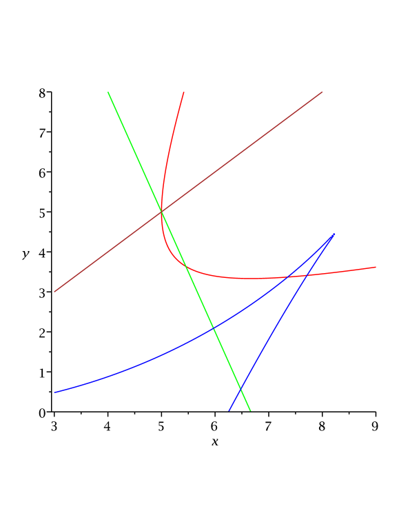
Figure 1. The sets $\mathcal{C}_{2}$, $\mathcal{C}_{5}$, $\{\beta=\gamma\}$ and $\mathcal{H}$.

Before proving Lemma 4 we finish the proof of Lemma 3. On Fig 1 we show the sets $\mathcal{C}_{2}$ (branch of a hyperbola), $\mathcal{C}_{5}$ (straight line with negative slope), the straight line $\{\beta=\gamma\}$ and $\mathcal{H}$ (curve with a cusp point) for $\alpha_{0}=5$. The set $\{c_{2}<0\}$ is the interior of the branch $\mathcal{C}_{2}$ and the set $\{c_{2}<0,c_{5}<0\}$ is the lens-shaped domain between $\mathcal{C}_{2}$ and $\mathcal{C}_{5}$. The point $I_{1}$ is the triple intersection of $\mathcal{C}_{2}$, $\mathcal{C}_{5}$ and $\{\beta=\gamma\}$.

Remark 1.

For $\alpha_{0}\in(1,\sqrt{3}]$ the set $\{c_{2}<0,c_{5}<0\}$ is not compact and for $\alpha_{0}\in(1,\sqrt{3})$ the point $I_{2}$ belongs not to $\mathcal{C}_{2}$, but to $\mathcal{C}_{2}^{*}$; $I_{2}$ is at $\infty$ for $\alpha_{0}=\sqrt{3}$. Indeed, the slopes of the asymptotes of the hyperbola $\{c_{2}=0\}$ equal $2\pm\sqrt{3}$ while the slope of $\mathcal{C}_{5}$ equals $2-\alpha_{0}$, see parts (1) and (2) of Lemma 4.

There exists a unique point $Z\in\mathcal{C}_{2}$ the tangent to $\mathcal{C}_{2}$ at which is horizontal. Indeed, the branches $\mathcal{C}_{2}$ and $\mathcal{C}_{2}^{*}$ of the hyperbola $\{c_{2}=0\}$ are symmetric w.r.t. its centre $(2\alpha_{0}/3,\alpha_{0}/3)$, see part (2) of Lemma 4. The only point of $\mathcal{C}_{2}^{*}$ at which the tangent line is horizontal is the origin, see part (2) of Lemma 4 (the fact that $(0,0)$ is the only such point follows from the convexity of the hyperbola). Hence $Z=(4\alpha_{0}/3,2\alpha_{0}/3)$.

Compare the $\gamma$-coordinates of the points $Z$ and $J$ (see part (4) of Lemma 4). For $\alpha_{0}<3\sqrt{2}=4.2\ldots$ one has $2\alpha_{0}/3>\alpha_{0}^{3}/27$. The point $Z$ has the least possible $\gamma$-coordinate of the points of $\mathcal{C}_{2}$ whereas $J$ has the largest possible $\gamma$-coordinate of the points of $\mathcal{H}\cap\mathcal{P}_{\alpha=\alpha_{0}}$, see part (4) of Lemma 4. Hence for $\alpha_{0}\in(1,3\sqrt{2})$ one has

$$\mathcal{C}_{2}\cap(\mathcal{H}\cap\mathcal{P}_{\alpha=\alpha_{0}})=\emptyset~{}~{}~{}\,\,{\rm and}~{}~{}~{}\,\,\{c_{2}<0,c_{5}<0\}\cap(\mathcal{H}\cap\mathcal{P}_{\alpha=\alpha_{0}})=\emptyset~{}.$$

Recall that $u_{0}<3\sqrt{2}$, see part (5) of Lemma 4. Hence for $\alpha_{0}=u_{0}$ the cusp $J$ of $\mathcal{H}$ has a smaller $\gamma$-coordinate than $I_{2}$. As $I_{2}$ does not belong to $\mathcal{H}$ (for any $\alpha_{0}>1$, see part (5) of Lemma 4), for $\alpha_{0}>u_{0}$ the points $I_{1}$ and $I_{2}$ are above the two intersection points $K_{1}$ and $K_{2}$ of $\mathcal{H}$ with $\mathcal{C}_{5}$ (“above” means “have larger $\gamma$-coordinates”); $K_{1}$ is presumed to be above $K_{2}$. Denote by $L^{*}$ and $L^{**}$ the vertical straight lines passing through $I_{2}$ and $K_{1}$. Hence for $a>3$ the domain $\{c_{2}<0,c_{5}<0\}$ lies to the left of $L^{*}$ and above $I_{2}$, see parts (1) and (3) of Lemma 4. At the same time the part of $\mathcal{H}\cap\mathcal{P}_{\alpha=\alpha_{0}}$ which is to the left of $L^{*}$ (hence to the left of $L^{**}$ as well) lies below $K_{1}$ hence below $I_{2}$, so the domain $\{c_{2}<0,c_{5}<0\}$ contains no hyperbolic polynomial. This proves Lemma 3 and Theorem 4. ∎

Proof of Lemma 4.

The first two statements of part (1) are to be checked directly. To prove the third statement it suffices to compute the intersection points of the line $\mathcal{C}_{5}$ with the $\beta$- and $\gamma$-axes. These points are $(0,\alpha_{0}(\alpha_{0}-1))$ and $(\alpha_{0}(\alpha_{0}-1)/(\alpha_{0}-2),0)$.

Prove part (2). The determinants of the matrices $M_{1}=\left(\begin{array}[]{rrr}1&-2&0\\ -2&1&\alpha_{0}\\ 0&\alpha_{0}&0\end{array}\right)$ and $M_{2}=\left(\begin{array}[]{rr}1&-2\\ -2&1\end{array}\right)$ (defined after the quadric $c_{2}|_{\alpha=\alpha_{0}}$) are nonzero and $M_{2}$ has one positive and one negative eigenvalue. Hence the equation $c_{2}=0$ defines a hyperbola. To find its centre one sets $\beta\mapsto\beta+\mu$, $\gamma\mapsto\gamma+\nu$ and one looks for $(\mu,\nu)$ such that the linear terms in the equation $c_{2}=0$ disappear. This yields the system

$$-4\mu+2\nu+2\alpha_{0}=0~{}~{}~{}~{},~{}~{}~{}~{}2\mu-4\nu=0$$

whose solution is $(\mu,\nu)=(2\alpha_{0}/3,\alpha_{0}/3)$. The slopes of the asymptotes are solutions to the equation $\lambda^{2}-4\lambda+1=0$ deduced from the matrix $M_{2}$. The branch $\mathcal{S}_{2}$ occupies the upper right sector defined by the asymptotes.

The equation $c_{2}=0$ is satisfied for $(\beta,\gamma)=(0,0)$. To compute the equation of the tangent line to the hyperbola $\{c_{2}=0\}$ one writes

(2.4) $$(-4\beta+2\gamma+2\alpha)d\gamma+(2\beta-4\gamma)d\beta=0$$

in which the coefficient of $d\beta$ is $0$ for $(\beta,\gamma)=(0,0)$. The tangent at $(0,0)$ being horizontal the branch $\mathcal{S}_{2}^{*}$ belongs entirely to the lower half-plane and does not intersect the set $\mathcal{P}|_{\alpha=\alpha_{0}}$.

Prove part (3). Set $B:=\gamma-\beta$, $A:=\beta-\alpha_{0}$. The conditions $c_{5}=0$ and $c_{2}=0$ read (see (2.2)):

$$B=-(\alpha_{0}-1)A~{}~{},~{}~{}-2(B+A+\alpha_{0})A+B^{2}=0$$

from which one finds that either $A=0$ (hence $B=0$ and $\beta=\gamma=\alpha_{0}$, this defines the point $I_{1}$) or $-2(-(\alpha_{0}-1)A+A+\alpha_{0})+(\alpha_{0}-1)^{2}A=0$. The last equality implies $A=2\alpha_{0}/(\alpha_{0}^{2}-3)$. Hence

(2.5) $$\beta=\alpha_{0}(\alpha_{0}^{2}-1)/(\alpha_{0}^{2}-3)~{},$$

so $B=2\alpha_{0}(1-\alpha_{0})/(\alpha_{0}^{2}-3)$ and

(2.6) $$\gamma=\alpha_{0}(\alpha_{0}-1)^{2}/(\alpha_{0}^{2}-3)~{}.$$

which gives the point $I_{2}$. To show that the tangent line to $\mathcal{C}_{2}$ at $I_{1}$ is vertical it suffices to observe that for $\beta=\gamma=\alpha_{0}$ equation (2.4) reduces to $d\beta=0$. At $I_{2}$ the tangent line to $\mathcal{C}_{2}$ is defined by the equation

$$(2\alpha_{0}^{2}/(\alpha_{0}^{2}-3))d\gamma+(\alpha_{0}(\alpha_{0}-1)(\alpha_{0}-3)/(\alpha_{0}^{2}-3))d\beta=0~{}.$$

Its slope equals $-(\alpha_{0}-1)(\alpha_{0}-3)/2\alpha_{0}$. The last statement of part (3) follows from the convexity of the hyperbola $\{c_{2}=0\}$.

To prove part (4) one has to recall that the real polynomial $x^{3}+px+q$ is hyperbolic if and only if $4p^{3}+27q^{2}\leq 0$ (this means, in particular, that $p\leq 0$). As

$$x^{3}+\alpha x^{2}+\beta x+\gamma=(x+\alpha/3)^{3}+(\beta-\alpha^{2}/3)(x+\alpha/3)+\gamma+2\alpha^{3}/27-\alpha\beta/3~{},$$

the polynomial $L|_{\alpha=\alpha_{0}}$ is hyperbolic if and only if condition (2.3) holds true.

Set $\beta\mapsto\alpha_{0}^{2}\beta$ and $\gamma\mapsto\alpha_{0}^{3}\gamma$ in the equation of $\mathcal{H}$ (see (2.3)). In the new variables $(\beta,\gamma)$ the equation of $\mathcal{H}$ (after division by $\alpha_{0}^{3}$) coincides with its equation for $\alpha_{0}=1$:

(2.7) $$4(\beta-1/3)^{3}+27(\gamma+2/27-\beta/3)^{2}=0~{}.$$

One can parametrize this curve by setting $\beta=1/3-3t^{2}$, $\gamma=1/27+2t^{3}-t^{2}=2(t-1/3)^{2}(t+1/6)$. It has a cusp for $t=0$, i.e. at $(1/3,1/27)$. Its tangent vector equals $(-6t,6t^{2}-2t)$. For $t<0$ its components are both positive and its slope is also positive. For $t\in(0,1/3)$ they are both negative and again the slope is positive. One has $\beta>0$ and $\gamma>0$ exactly when $t\in(-1/6,1/3)$ (i.e. only for values of $t$ for which the slope is positive). The coordinate $\beta$ attains its global maximal value $1/3$ only for $t=0$. For $t\in(-1/6,1/3)$ the coordinate $\gamma$ attains its maximal value $1/27$ only for $t=0$.

Prove part (5). The equation of $\mathcal{H}$ with $\gamma=\beta-(\alpha_{0}-1)(\beta-\alpha_{0})$ reads:

(2.8) $$\begin{array}[]{ccl}\mathcal{U}(\alpha_{0},\beta)&:=&4\beta^{3}+44\beta^{2}\alpha_{0}^{2}-4\beta\alpha_{0}^{4}-108\alpha_{0}\beta+27\alpha_{0}^{2}-54\alpha_{0}^{3}\\ &&+108\beta^{2}+180\beta\alpha_{0}^{2}-144\alpha_{0}\beta^{2}-64\beta\alpha_{0}^{3}+23\alpha_{0}^{4}+4\alpha_{0}^{5}=0~{}.\end{array}$$

One has

$${\rm Res}(\mathcal{U},\partial\mathcal{U}/\partial\beta,\beta)=-64\alpha_{0}^{3}(\alpha_{0}-1)(2\alpha_{0}^{2}-7\alpha_{0}+8)(10\alpha_{0}^{2}-45\alpha-0+27)^{3}~{}.$$

The first quadratic factor has no real roots. The roots of the second one equal $0.7129573851\ldots<1$ and $u_{0}:=3.787042615\ldots$. For $\alpha_{0}=u_{0}$ the cusp point of $\mathcal{H}$ is on $\mathcal{C}_{5}$. For $\alpha_{0}<u_{0}$ the curve $\mathcal{H}\cap\mathcal{P}|_{\alpha=\alpha_{0}}$ lies entirely below the line $\mathcal{C}_{5}$ (this can be deduced from the last statement of part (4) of the lemma and from the fact that for $\alpha_{0}>0$ small enough the cusp point $J$ is close to the origin); for $\alpha_{0}>u_{0}$ it intersects this line at two points.

Remark 2.

Equation (2.8) is of degree $3$ w.r.t. $\beta$. On Fig. 1 one sees two of the solutions (the points $K_{1}$ and $K_{2}$, see the proof of Lemma 3). The third solution is an intersection point of $\mathcal{H}$ with $\mathcal{C}_{5}$, with $\beta<0$ and $\gamma>0$. Such an intersection point exists because the $\gamma$-coordinate of a point of $\mathcal{C}_{5}$ grows linearly in $|\beta|$ as $|\beta|$ increases ($\beta$ being negative) while the $\gamma$-coordinate of a point of $\mathcal{H}$ grows as $|\beta|^{3/2}$.

To prove the last statement of part (5) we substitute the right-hand sides of (2.5) and (2.6) for $\beta$ and $\gamma$ in (2.3) and we multiply by $(\alpha_{0}^{2}-3)^{3}/\alpha_{0}^{2}(\alpha_{0}-1)^{2}>0$. This yields the equivalent condition

$$3\alpha_{0}^{6}-16\alpha_{0}^{5}+13\alpha_{0}^{4}+24\alpha_{0}^{3}-23\alpha_{0}^{2}+104\alpha_{0}-81\leq 0~{}.$$

However the left-hand side has no roots greater than $1$ and the leading coefficient is positive. Hence the last inequality fails for $\alpha_{0}>1$.

∎

3. Cases 2 - 6 are not realizable

3.1. Preliminaries

The following two lemmas are proved in the Appendix. They allow to simplify the proof of Theorem 3 by decreasing the number of parameters.

Lemma 5.

Suppose that there exists a monic degree $8$ polynomial $P$ realizing Case $j$, $2\leq j\leq 6$. Then there exists a monic degree $8$ polynomial $U$ having a quadruple root at $1$ and no other real roots, and whose coefficients define the same sign pattern as the one of Case $j$.

Remark 3.

One can observe that roots at $1$ remain invariant under reverting of sign patterns.

Lemma 6.

(1) Suppose that a monic polynomial $U=(x-1)^{4}V$ realizes one of the sign patterns

$$\begin{array}[]{lllllll}\sigma_{2}^{r}&=&(+,+,-,-,-,+,-,+,+)&{}{}{}{}{}{}{}{}{}&\sigma_{4}&=&(+,+,+,-,-,+,-,+,+)\\ &&~{}~{}~{}~{}~{}{\rm or}&&\sigma_{6}^{r}&=&(+,-,-,-,-,+,-,+,+)~{},\end{array}$$

where $V$ is a real monic polynomial with no real root. Then there exists a polynomial of the form $U_{t}:=U-t(x-1)^{4}$, $t\geq 0$, defining the same sign pattern and having one or two negative roots of even multiplicity, hence a polynomial of the form

(3.9) $$W:=(x-1)^{4}(x^{2}+Sx+S^{2}/4)(x^{2}+Mx+N)~{},~{}~{}{\rm where}~{}~{}S>0~{}~{}{\rm and}~{}~{}N\geq M^{2}/4~{}.$$

(2) If the polynomial $U$ realizes the sign pattern $\sigma_{3}^{r}=(+,-,-,+,-,+,-,+,+)$, then in the family of polynomials $U^{*}_{t}:=U+tx(x-1)^{4}$, $t>0$, there exists a polynomial defining the sign pattern $\sigma_{3}^{r}$ and of the form (3.9).

(3) If the polynomial $U$ realizes the sign pattern $\sigma_{5}^{r}=(+,-,-,+,-,+,+,+,+)$, then in the family of polynomials $U^{*}_{t}:=U+tx(x-1)^{4}$, $t>0$, there exists a polynomial defining one of the sign patterns $\sigma_{3}^{r}$, $\sigma_{5}^{r}$ or $\sigma^{*}:=(+,-,-,+,-,+,0,+,+)$ and of the form (3.9).

In what follows we set $W:=\sum_{j=0}^{8}w_{j}x^{j}$, $w_{8}=1$, and

$$Q:=3S^{2}/2-4S+1~{}~{},~{}~{}R:=S^{2}-6S+4~{}~{}{\rm and}~{}~{}P:=S^{2}/4-4S+6~{}.$$

The roots of these three polynomials are real. We denote them by

$$\begin{array}[]{ccccccccccc}0.27\ldots&=&(4-\sqrt{10})/3&=&q_{1}&<&q_{2}&=&(4+\sqrt{10})/3&=&2.38\ldots\\ 0.76\ldots&=&3-\sqrt{5}&=&r_{1}&<&r_{2}&=&3+\sqrt{5}&=&5.23\ldots\\ 1.67\ldots&=&8-\sqrt{40}&=&p_{1}&<&p_{2}&=&8+\sqrt{40}&=&14.32\ldots\end{array}$$

The coefficients $w_{j}$, $j=0$, $\ldots$, $7$ are expressed by the following formulae:

(3.10) $$\begin{array}[]{ccccccc}w_{0}&=&S^{2}N/4&&w_{1}&=&(S/4)(MS+4N(1-S))\\ w_{2}&=&QN+(S-S^{2})M+S^{2}/4&&w_{3}&=&QM-RN+S-S^{2}\\ w_{4}&=&Q-RM+PN&&w_{5}&=&-R+PM+(S-4)N\\ w_{6}&=&P+(S-4)M+N&&w_{7}&=&M+S-4\end{array}$$

3.2. Cases 2 and 4

In Cases 2 and 4 we are using the sign patterns $\sigma_{2}^{r}=(+,+,-,-,-,+,-,+,+)$ and $\sigma_{4}=(+,+,+,-,-,+,-,+,+)$. They can be united in a single sign pattern $\pi_{\pm}:=(+,+,\pm,-,-,+,-,+,+)$. If the polynomial $W$ (see (3.9) defines the sign pattern $\pi_{\pm}$, then one must have $w_{j}>0$ for $j=0$, $1$, $3$ and $7$ and $w_{j}<0$ for $j=2$, $4$ and $5$.

One has $M>0$. Indeed, $w_{7}=M+S-4>0$, hence $S>4-M$. Suppose that $M\leq 0$. Then one has $S>4$, $MS\leq 0$ and $4N(1-S)\leq 0$, i.e. $w_{1}\leq 0$ – a contradiction.

Suppose that $S>1$. Then the condition $w_{1}>0$ is equivalent to $N<MS/4(S-1)$. On the other hand, as $N\geq M^{2}/4$, the last two inequalities together imply $M<S/(S-1)$ hence $N<S^{2}/u$, where $u=4(S-1)^{2}$.

For $S\in[p_{1},p_{2}]$ (recall that $p_{1}>1$) one has $P\leq 0$, $PN\geq PS^{2}/u$ and $4-S<M<S/(S-1)$. Therefore

$$w_{4}\geq\min(~{}Q(S)-R(S)(4-S)+P(S)S^{2}/u~{},~{}Q(S)-R(S)S/(S-1)+P(S)S^{2}/u~{})~{}.$$

This minimum is $>5$ hence $>0$ (the numerical check of this is easy) and the inequality $w_{4}<0$ fails for $S\in[p_{1},p_{2}]$.

For $S>p_{2}$ one has $P\geq 0$, $PN\geq PM^{2}/4\geq 0$ and $0<M<S/(S-1)$, so

$$w_{4}\geq\min(~{}Q(S)-R(S)S/(S-1)~{},~{}Q(S)~{})~{}.$$

This minimum is also positive and again $w_{4}<0$ fails.

Let now $S\in(0,p_{1})$. The inequality $w_{4}<0$ can be rewritten as $N<(RM-Q)/P$ which together with $M^{2}/4\leq N$ implies $PM^{2}-4RM+4Q<0$. This is a quadratic inequality w.r.t. $M$, with $P>0$. The discriminant of the quadratic polynomial $Y(M,S):=P(S)M^{2}-4R(S)M+4Q(S)$ equals $4(R^{2}(S)-P(S)Q(S))$. It is positive for all $S\in(0,p_{1})$ (this is easy to check). Hence for $S\in(0,p_{1})$ the polynomial $Y$ has two real roots $M^{\prime}<M^{\prime\prime}$ which depend continuously on $S$ and one must have $M\in(M^{\prime},M^{\prime\prime})$.

For each $S\in(0,p_{1})$ fixed both these roots are smaller than $4-S$. Indeed, set $M:=4-S$. The polynomial $Y(4-S,S)$ is positive on $(0,p_{1})$ (easy to check). For $S=1\in(0,p_{1})$ one has $Q=-3/2<0$, i.e. one of the roots is negative and the other is positive. Hence for $S\in(0,p_{1})$ the number $4-S$ lies outside the interval $[M^{\prime},M^{\prime\prime}]$, and as $4-S>0$, one has $M^{\prime}<4-S$, $M^{\prime\prime}<4-S$ and $M\in(M^{\prime},M^{\prime\prime})$. But one must have $M>4-S$, so the inequalities $w_{7}>0$ and $w_{4}<0$ cannot hold simultaneously for $S\in(0,p_{1})$.

3.3. Cases 3, 5 and 6

In Cases 3, 5 and 6 we use the sign patterns

$$\begin{array}[]{lllllll}\sigma_{3}^{r}&=&(+,-,-,+,-,+,-,+,+)&~{}~{}~{}~{},&\sigma_{5}^{r}&=&(+,-,-,+,-,+,+,+,+)\\ &&{\rm and}&&\sigma_{6}^{r}&=&(+,-,-,-,-,+,-,+,+)~{}.\end{array}$$

and formulae (3.10). The proof of Theorem 4 in these cases results from Lemmas 8, 9 and 10.

Lemma 7.

In Cases 3, 5 and 6 one has $M>0$.

Proof.

One must have $w_{1}>0$ and $w_{6}<0$. For $S\geq 1$ the product $N(1-S)$ is negative (see formulae (3.10)), so for $S\geq 1$ the condition $w_{1}>0$ implies that one must have $SM>0$, i.e. $M>0$. Consider for $S\in(0,1)$ the condition $w_{6}<0$, (i.e. $P+(S-4)M+N<0$). One has $P(S)>0$, $N\geq 0$ and $S-4<0$, so the inequality $w_{6}<0$ is possible only for $M>0$. ∎

Lemma 8.

Cases 3, 5 and 6 are not realizable for $S\in(0,r_{1}]$.

Proof.

In Cases 3, 5 and 6 one has $w_{3}>0$, i.e. $QM+S-S^{2}>RN$, see (3.10). For $S\in(0,r_{1}]$ one has $R(S)\geq 0$ and $QM+S-S^{2}>RN\geq RM^{2}/4$, hence

(3.11) $$L(S,M):=R(S)M^{2}/4-Q(S)M-S+S^{2}<0~{}.$$

The inequalities (3.11), $0<S\leq r_{1}$ and $0\leq M<4-S$ have no common solution. Indeed, $L(S,4-S)=(S-2)^{2}((S-2)^{2}+8)/4$. This means that for $S=2$ the line $M+S=4$ has an ordinary tangency with the curve $L(S,M)=0$, and this is their only common point in the domain $\{S>0,M>0\}$. For $S=M=1/2$ one has $L(S,M)=9/64>0$ and $S+M-4<0$. Hence below the line $M+S=4$ in the domain $\{S>0,M>0\}$ one has $L(S,M)>0$. ∎

Remark 4.

(1) The inequalities $S>0$, $M>0$ (see Lemma 7) and $S+M<4$ (this follows from $w_{7}<0$ in Cases 3, 5 and 6) imply $S<4$.

Convention 1.

(1) In what follows we interpret an equality of the form $w_{j}=0$ (see (3.10)) as the equation of a straight line (denoted by $\ell_{j}$) in the space $(M,N)$ with coefficients depending on $S$ as on a parameter. Most often we need equations of the form $A(S)N+B(S)M+C(S)=0$, and we care to have a positive coefficient of $N$. E.g. we prefer the equation of the line $\ell_{1}$ (see the quantity $w_{1}$ in formulae (3.10)) to be of the form $4(1-S)N+SM=0$ for $S<1$ and $4(S-1)N-SM=0$ for $S>1$.

(2) We denote by $\ell_{j}^{+}$ (resp. $\ell_{j}^{-}$) the upper (resp. lower) half-plane defined by the line $\ell_{j}$. In the case of $\ell_{1}$ one has $\ell_{1}^{+}:4(1-S)N+SM>0$ for $S<1$ and $\ell_{1}^{+}:4(S-1)N-SM>0$ for $S>1$. For $S=1$ this line is vertical and we do not define the half-planes $\ell_{1}^{\pm}$. By $s(\ell_{j})$ we denote the slope of the line $\ell_{j}$, i.e. the quantity $-B(S)/A(S)$ for $A(S)\neq 0$. For $\ell_{1}$ it equals $S/4(S-1)$.

(3) When in the proofs of the lemmas rational functions appear, it is presumed that the factors of degree $2$ have no real roots (so their sign coincides with the one of their leading coefficient). Factorizations are performed by means of MAPLE.

Lemma 9.

Cases 3, 5 and 6 are not realizable for $S\in[p_{1},4)$.

Proof.

Consider the four conditions $M>0$, $w_{1}>0$, $w_{3}>0$ and $w_{4}<0$. The second of them defines the half-plane $\ell_{1}^{-}$ (recall that $\ell_{1}:4(S-1)N-SM=0$). The last two of them read

$$(-R(S))N+Q(S)M+S-S^{2}>0\hskip 17.07164pt{\rm and}\hskip 17.07164pt(-P(S))N+R(S)M-Q(S)>0~{}.$$

The straight line $\ell_{3}:(-R(S))N+Q(S)M+S-S^{2}=0$ intersects the $N$-axis at the point $A:=(0,N_{A})$ with $N_{A}:=S(S-1)/(-R(S))>0$. The lines $\ell_{3}$ and $\ell_{4}:(-P(S))N+R(S)M-Q(S)=0$ intersect at the point $B$ with coordinates

$$\begin{array}[]{lllll}M_{B}&:=&(2/5)(5S^{4}-35S^{3}+84S^{2}-64S+16)/K(S)&,&\\ N_{B}&:=&(2/5)(5S^{4}-20S^{3}+36S^{2}-16S+4)/K(S)&,&{\rm where}\\ K(S)&:=&S^{4}-8S^{3}+30S^{2}-32S+16&.\end{array}$$

and both numerators and the denominator $K$ have no real roots. This point lies above the straight line $\ell_{1}$. Indeed, the coefficient of $N$ in the equation of $\ell_{1}$ is positive. Substituting $(M_{B},N_{B})$ for $(M,N)$ in the left-hand side of this equation yields the expression

$$\mu:=\frac{6(S^{2}-2.5\ldots S+3.8\ldots)(S^{2}-0.5\ldots S+0.2\ldots)(S-1.2\ldots)}{(S^{2}-6.6\ldots S+20.4\ldots)(S^{2}-1.3\ldots S+0.7\ldots)}~{}$$

which is positive, see Convention 1.

For the slopes $s(\ell_{4})$ and $s(\ell_{1})$ one has $s(\ell_{4})>s(\ell_{1})>0$. The first inequality follows from $R(S)/P(S)-S/4(S-1)>0$ which is equivalent to

$$\frac{15(S^{2}-1.7\ldots S+0.9\ldots)(S-4.6\ldots)}{4P(S)(S-1)}>0$$

and this results from $S-4.6\ldots<0$, $S-1>0$ and $P(S)<0$.

Hence the set defined by the conditions $M>0$, $w_{3}>0$ and $w_{4}<0$ is the domain of $\mathbb{R}^{2}\simeq(M,N)$ to the right of the $N$-axis, to the above of the segment $AB$ and to the above of the half-line starting at $B$, which is part of the line $\ell_{4}$ and which goes to the right and upward. This domain does not intersect the half-plane $\ell_{1}^{-}$ and the four conditions $M>0$, $w_{1}>0$, $w_{3}>0$ and $w_{4}<0$ cannot hold true simultaneously. ∎

Lemma 10.

Cases 3, 5 and 6 are not realizable for $S\in(r_{1},p_{1})$.

Proof.

Consider the conditions $w_{3}>0$ and $w_{6}<0$. They read

$$(-R(S))N+Q(S)M+S-S^{2}>0\hskip 17.07164pt{\rm and}\hskip 17.07164ptN+(S-4)M+P(S)<0~{}.$$

Consider the point $\Pi:=\ell_{3}\cap\ell_{6}$. Its coordinates equal

$$(-(S^{4}-22S^{3}+120S^{2}-204S+96)/2Y(S),-3(S^{4}-16S^{3}+54S^{2}-64S+16)/4Y(S))~{},$$

where $Y(S):=2S^{3}-17S^{2}+48S-30$ has a single real root $y_{0}:=0.8609094817\ldots$. For $S\in(r_{1},y_{0})$ (resp. for $S\in(y_{0},p_{1})$) one has $s(\ell_{3})>s(\ell_{6})$ (resp. $s(\ell_{3})<s(\ell_{6})$). This follows from

$$Q(S)/R(S)-(4-S)=(S^{2}-7.6\ldots S+17.4\ldots)(S-y_{0})/R(S)$$

with $R(S)<0$. The second coordinate of $\Pi$ equals

$$-3(S-0.3\ldots)(S-11.9\ldots)(S^{2}-3.7\ldots S+4.0\ldots)/4Y(S)~{}.$$

Hence it changes sign from $-$ to $+$ when $S$ passes from $y_{0}^{-}$ to $y_{0}^{+}$. For $S\in(r_{1},y_{0})$ one has $\{w_{3}>0\}\cap\{w_{6}<0\}=\ell_{3}^{+}\cap\ell_{6}^{-}$. For $S=y_{0}$ the lines $\ell_{3}$ and $\ell_{6}$ are parallel, $\ell_{3}$ is above $\ell_{6}$ and $\{w_{3}>0\}\cap\{w_{6}<0\}=\emptyset$. Thus for $S\in(r_{1},y_{0})$ the sector $\ell_{3}\cap\ell_{6}$ belongs to the domain $N<0$ and if some of Cases 3, 5 or 6 is realizable, it can be realizable only for $S\in(y_{0},p_{1})$.

For $S=y_{0}^{+}$ the intersection $\{w_{3}>0\}\cap\{w_{6}<0\}$ is a sector whose vertex has both coordinates positive because the first coordinate of $\Pi$ equals

$$-(S-0.7\ldots)(S-1.8\ldots)(S-4.6\ldots)(S-14.7\ldots)/2Y(S)>0~{}.$$

The point $\Pi$ lies above the line $\ell_{4}:P(S)N-R(S)M+Q(S)=0$ for $S\in(y_{0},y_{1})$, where $y_{1}:=1.471576286\ldots$. Indeed, substituting the coordinates of $\Pi$ for $(M,N)$ in the left-hand side of the equation of $\ell_{4}$ yields

$$\frac{5(S^{2}-5.2\ldots S+20.3\ldots)(S^{2}-1.2\ldots S+1.2\ldots)(S-7.9\ldots)(S-y_{1})}{32(S^{2}-7.6\ldots S+17.4\ldots)(S-y_{0})}>0~{}.$$

Moreover, $s(\ell_{4})<0<s(\ell_{3})<s(\ell_{6})$. Hence for $S\in(y_{0},y_{1})$ the three conditions $w_{3}>0$, $w_{4}<0$ and $w_{6}<0$ cannot hold true simultaneously.

In order to prove the lemma for $S\in[y_{1},p_{1})$ we consider the conditions

$$w_{1}>0~{}~{}{\rm,~{}~{}i.e.}~{}~{}4(S-1)N-MS<0~{}~{}~{}{\rm and}~{}~{}~{}w_{3}>0~{}~{}{\rm,~{}~{}i.e.}~{}~{}-R(S)N+Q(S)M+S-S^{2}>0~{}.$$

The point $\Gamma:=\ell_{1}\cap\ell_{3}$ has coordinates $(M_{\Gamma},N_{\Gamma})$ which equal

$$(4(S-1)^{2}S/(5S^{3}-16S^{2}+16S-4)~{},~{}S^{2}(S-1)/(5S^{3}-16S^{2}+16S-4))~{}.$$

Both coordinates are positive for $S\in[y_{1},p_{1})$ (the only real zero of the denominator equals $0.3\ldots$). The point $\Gamma$ lies above the straight line $\ell_{4}$. Indeed, substituting $(M_{\Gamma},N_{\Gamma})$ for $(M,N)$ in the left-hand side of the equation of $\ell_{4}:P(S)N-R(S)M+Q(S)=0$ with $P(S)>0$ yields

$$\frac{3(S^{2}-2.5\ldots S+3.8\ldots)(S^{2}-0.5\ldots S+0.2\ldots)(S-1.2\ldots)}{4(S^{2}-2.8\ldots S+2.1\ldots)(S-0.3\ldots)}>0~{}.$$

One has $s(\ell_{4})<0<s(\ell_{3})<s(\ell_{1})$; the last inequality follows from

$$\frac{S}{4(S-1)}-\frac{Q(S)}{R(S)}=-\frac{5(S^{2}-2.8\ldots S+2.1\ldots)(S-0.3\ldots)}{4(S-5.2\ldots)(S-1)(S-0.7\ldots)}>0~{}.$$

Hence for $S\in[y_{1},p_{1})$ the sector $\{w_{1}>0\}\cap\{w_{3}>0\}$ does not intersect the half-plane $\{w_{4}<0\}=\ell_{4}^{-}$, i.e. the three conditions $w_{1}>0$, $w_{3}>0$ and $w_{4}<0$ do not hold simultaneously. ∎

4. Appendix. Proofs of Lemmas 5 and 6

Proof of Lemma 5.

Denote by $0<x_{1}<x_{2}<x_{3}<x_{4}$ the real roots of $P$. We are looking first for a polynomial $U^{0}(x)$ of the form $(P(x)+ax^{8}-bx^{k}+c)/(1+a)$ having a quadruple root $x_{0}>0$, where $k=1$ in Cases 3, 5 and 6, $k=3$ in Case 2, $k=5$ in Case 4, and $a>0$, $b>0$, $c>0$. The signs of $a$, $b$ and $c$ imply that $U^{0}$ defines the same sign pattern as $P$. The polynomial $U$ is obtained from $U^{0}$ by suitable rescaling and multiplication by a positive constant which does not change the sign pattern.

For $x=x_{0}$ the polynomial $U^{0}$ satisfies the conditions $(U^{0})^{\prime}=(U^{0})^{\prime\prime}=(U^{0})^{\prime\prime\prime}=0$ which read:

(4.12) $$\begin{array}[]{lll}~{}~{}k=1&&\\ P^{\prime}(x)+8ax^{7}-b=0&P^{\prime\prime}+56ax^{6}=0&P^{\prime\prime\prime}+336ax^{5}=0\\ ~{}~{}k=3&&\\ P^{\prime}(x)+8ax^{7}-3bx^{2}=0&P^{\prime\prime}+56ax^{6}-6bx=0&P^{\prime\prime\prime}+336ax^{5}-6b=0\\ ~{}~{}k=5&&\\ P^{\prime}(x)+8ax^{7}-5bx^{4}=0&P^{\prime\prime}+56ax^{6}-20bx^{3}=0&P^{\prime\prime\prime}+336ax^{5}-60bx^{2}=0\end{array}$$

Consider first Cases 5 and 6, hence $k=1$. One eliminates $a$ from the last two equations which gives $xP^{\prime\prime\prime}(x)=6P^{\prime\prime}(x)$. The polynomial $P^{\prime}$ has exactly three positive roots $\mu_{1}<\mu_{2}<\mu_{3}$, $\mu_{j}\in(x_{j},x_{j+1})$. Indeed, by Rolle’s theorem it has at least three and by Descartes’ rule of signs it has at most three of them. So for $x>x_{4}$ (resp. $x>\mu_{3}$) the polynomial $P$ (resp. $P^{\prime}$) is positive.

The polynomial $P^{\prime\prime}$ has at least two real roots $\xi_{1}<\xi_{2}$, $\xi_{j}\in(\mu_{j},\mu_{j+1})$ (again by Rolle’s theorem). By Descartes’ rule of signs the polynomial $P^{\prime\prime}$ has at most three positive roots. The sign of the coefficient of $x^{2}$ in $P$ is negative, therefore $P^{\prime\prime}$ has exactly three positive roots. The third of them $\xi_{3}$ is in $(0,\xi_{1})$. Indeed, to the right of $\xi_{2}$ the number of positive roots of $P^{\prime\prime}$ must be even because for $x>0$ sufficiently large $P$ is convex. So $0<\xi_{3}<\xi_{1}<\xi_{2}$.

The polynomial $P^{\prime\prime\prime}$ has real roots $\zeta_{1}\in(\xi_{3},\xi_{1})$ and $\zeta_{2}\in(\xi_{1},\xi_{2})$. By Descartes’ rule of signs it has at most three positive roots in Case 6 and at most two in Case 5. In Case 6, as $P^{\prime\prime\prime}$ must have an even number of roots to the right of $\xi_{2}$ ($P^{\prime}$ is convex for $x>0$ sufficiently large), the three positive roots $\zeta_{3}<\zeta_{1}<\zeta_{2}$ of $P^{\prime\prime\prime}$ belong respectively to the intervals $(0,\xi_{3})$, $(\xi_{3},\xi_{1})$ and $(\xi_{1},\xi_{2})$.

Hence the signs of $P^{\prime\prime\prime}(\xi_{1})$ and $P^{\prime\prime\prime}(\xi_{2})$ are opposite and $xP^{\prime\prime\prime}-6P^{\prime\prime}$ changes sign at some point $x_{0}\in(\xi_{1},\xi_{2})$.

In Case 3 one has again $k=1$. The sign patterns $\sigma_{3}$ and $\sigma_{5}$ differ only in their third position. The proof resembles the one in Cases 5 and 6 yet Descartes’ rule of signs allows more positive roots for $P^{\prime}$, $P^{\prime\prime}$ and $P^{\prime\prime\prime}$.

Denote by $p(P^{\prime})$ the number of positive roots of $P^{\prime}$. Combining Rolle’s theorem and Descartes’ rule of signs one understands that it is possible to encounter only one of the following triples $(p(P^{\prime}),p(P^{\prime\prime}),p(P^{\prime\prime\prime}))$:

$$i)~{}(3,5,4)\hskip 28.45274ptii)~{}(3,3,4)\hskip 28.45274ptiii)~{}(3,3,2)\hskip 28.45274ptiv)~{}(5,5,4)~{}.$$

In case iii) the proof is carried out in exactly the same way as for Case 5. In the other cases one performs analogous reasoning with only difference the two more positive roots of $P^{\prime\prime}$ and $P^{\prime\prime\prime}$ in case i), of $P^{\prime\prime\prime}$ in case ii) or of $P^{\prime}$, $P^{\prime\prime}$ and $P^{\prime\prime\prime}$ in case iv). For parity reasons the two more roots of the corresponding derivative $P^{(j)}$ (compared to their number in the proof of Case 5) must belong to one and the same interval of $[0,\infty)$ defined by $0$, $\infty$ and the positive roots of $P^{(j-1)}$. One proves as for Case 5 that the signs of $P^{\prime\prime\prime}$ at two consecutive roots of $P^{\prime\prime}$ are opposite, hence $xP^{\prime\prime\prime}-6P^{\prime\prime}$ changes sign at some point $x_{0}$ from the interval between these two roots.

Consider Case 2, hence $k=3$. Eliminating $b$ from equations (4.12) yields:

$$2P^{\prime}-xP^{\prime\prime}=40ax^{7}~{}~{}{\rm and}~{}~{}P^{\prime\prime}-xP^{\prime\prime\prime}=280ax^{6}~{}.$$

Eliminating $a$ from the last two equations gives the equation

$$14P^{\prime}-8xP^{\prime\prime}+x^{2}P^{\prime\prime\prime}=(14P^{\prime}-2xP^{\prime\prime})-(x/2)(14P^{\prime}-2xP^{\prime\prime})^{\prime}=0~{}.$$

The polynomial $P^{\prime}$ has at most four positive roots (by Descartes’ rule of signs), and at least three of them (denoted by $\mu_{j}$) belong to the intervals $(x_{j},x_{j+1})$, $j=1$, $2$ and $3$, hence the fourth one $\mu_{0}$ is in $(0,x_{1})$ (because $P^{\prime}(0)>0$). The polynomial $P^{\prime\prime}$ has positive roots $\xi_{\nu}\in(\mu_{\nu},\mu_{\nu+1})$, $\nu=1$, $2$, and $\xi_{0}\in(\mu_{0},\mu_{1})$. Hence the polynomial $S:=14P^{\prime}-2xP^{\prime\prime}$ has different signs at $\mu_{\nu}$ and $\mu_{\nu+1}$ for $\nu=1$ and $2$, hence it has roots $\delta_{\nu}\in(\mu_{\nu},\mu_{\nu+1})$, its derivative has opposite signs at $\delta_{1}$ and $\delta_{2}$, so $S-(x/2)S^{\prime}:=14P^{\prime}-8xP^{\prime\prime}+x^{2}P^{\prime\prime\prime}$ has a real root $x_{0}\in(\mu_{1},\mu_{3})$.

Consider Case 4, hence $k=5$. One first eliminates $b$ (see equations (4.12)):

$$4P^{\prime}-xP^{\prime\prime}=24ax^{7}~{}~{}\,\,{\rm and}~{}~{}\,\,3P^{\prime\prime}-xP^{\prime\prime\prime}=168ax^{6}~{}.$$

Eliminating after this $a$ results in

$$28P^{\prime}-10xP^{\prime\prime}+x^{2}P^{\prime\prime\prime}=(28P^{\prime}-4xP^{\prime\prime})-(x/4)(28P^{\prime}-4xP^{\prime\prime})^{\prime}=0~{}.$$

Similarly to the proof in Case 2 one shows that the polynomial $28P^{\prime}-10xP^{\prime\prime}+x^{2}P^{\prime\prime\prime}$ has a positive root $x_{0}$.

After the number $x_{0}$ is found, one finds first $a$ and then $b$ from system (4.12). Now we have to justify the positive signs of $a$ and $b$ (and after this the one of $c$ as well). To this end we set $a=ta_{*}$, $b=tb_{*}$, where $t>0$, and we consider the family of polynomials $R_{t}(x):=P(x)+t\psi_{k}(x)$ with $\psi_{k}:=a_{*}x^{8}-b_{*}x^{k}$, $k=1$, $3$ or $5$. We suppose that for some $t>0$ the polynomial $R_{t}$ has a triple critical point at $x_{0}$. Hence for a suitably chosen $c$ the polynomial $R_{t}+c$ has a quadruple root at $x_{0}$.

Consider the function $\psi_{k}$ for $x>0$. For $a_{*}\geq 0$, $b_{*}\leq 0$ and $a_{*}-b_{*}>0$ it is increasing and convex, for $a_{*}\leq 0$, $b_{*}\geq 0$ and $a_{*}-b_{*}<0$ it is decreasing and concave (for $a_{*}=0$ and $k=1$ it is linear, i.e. convex and concave at the same time). For $a_{*}>0$ and $b_{*}>0$ (resp. for $a_{*}<0$ and $b_{*}<0$) it has a minimum (resp. a maximum) at $\lambda_{k}:=(kb_{*}/8a_{*})^{1/(8-k)}$ with $\psi_{k}(x)<0$ for $x\in(0,\lambda_{k}]$ (resp. with $\psi_{k}(x)>0$ for $x\in(0,\lambda_{k}]$).

Consider the family of polynomials $R_{t}$, where $t$ is supposed to belong to an interval $[0,\alpha)$ such that the sign pattern defined by the coefficients of $R_{t}$ is the one of $P$. We keep the same notation for the positive roots of $R_{t}$ and its derivatives as the one for $P$. Then:

A) If $\psi_{k}$ is decreasing on $[\mu_{2},\mu_{3}]$, then as $t$ increases, $\mu_{2}$ moves to the left and $\mu_{3}$ to the right;

B) If $\psi_{k}$ is increasing on $[\mu_{1},\mu_{2}]$, then as $t$ increases, $\mu_{1}$ moves to the left and $\mu_{2}$ to the right.

In both cases A) and B) it is impossible to have the three positive roots of $R_{t}^{\prime}$ coalescing into a single critical point of $R_{t}$. If $a_{*}\geq 0$, $b_{*}\leq 0$ and $a_{*}-b_{*}>0$, then case B) takes place. If $a_{*}\leq 0$, $b_{*}\geq 0$ and $a_{*}-b_{*}<0$, then case A) takes place. If $a_{*}<0$ and $b_{*}<0$, then at least one of cases A) or B) takes place. Hence only for $a_{*}>0$ and $b_{*}>0$ can one have a critical point of $R_{t}$ of multiplicity $3$. This implies that $a>0$ and $b>0$. Besides, $\lambda_{k}\in(\mu_{1},\mu_{3})$. Hence $R_{t}(\mu_{1})<0$ (because $P(\mu_{1})<0$ and $\psi_{k}(\mu_{1})<0$) and to have $U^{0}(x_{0})=0$ one has to choose $c>0$. ∎

Proof of Lemma 6.

Prove part (1). Consider the one-parameter family of polynomials $U_{t}:=U-t(x-1)^{4}$, $t\geq 0$. The first four coefficients do not depend on $t$ (they are the same as the ones of $U$). The signs of the five coefficients of $-(x-1)^{4}$ are $(-,+,-,+,-)$. Hence the first $8$ components of the sign pattern of $U_{t}$ do not depend on $t$ and in the family $U_{t}$ for some $t>0$, due to the decreasing of the value of $U_{t}$ as $t$ increases, one of the two things takes place first:

a) one has $U_{t}(0)=0$ or

b) $U_{t}$ has one or two negative roots, each of them of even multiplicity.

One can notice that the family $U_{t}$ contains no polynomial with six positive roots (counted with multiplicity) because there are four or five sign changes in the sign pattern of $U_{t}$ (the sign pattern of $U_{t}$ is obtained from $\sigma_{2}^{r}$, $\sigma_{4}$ or $\sigma_{6}^{r}$ by replacing the last component by $+$, $0$ or $-$).

If a) takes place for $t_{0}>0$, then as $U_{t}^{\prime}(0)>0$, the root of $U_{t}$ at $0$ is simple and $U_{t}$ has one or several negative roots whose total multiplicity is odd. Hence for some $t_{1}\in(0,t_{0})$, b) has taken place. Therefore in the family $U_{t}$ there exists (for some $t>0$) a polynomial of the form (3.9) which realizes the pattern $\sigma_{2}^{r}$, $\sigma_{4}$ or $\sigma_{6}^{r}$.

Prove part (2) of the lemma. Suppose that the polynomial $U$ realizes the sign pattern $\sigma_{3}^{r}=(+,-,-,+,-,+,-,+,+)$. Consider the family $U^{*}_{t}=U+tx(x-1)^{4}$, $t>0$. The signs of the coefficients of $x(x-1)^{4}$ are $(0,0,0,+,-,+,-,+,0)$, so the sign pattern of $U^{*}_{t}$ is $\sigma_{3}^{r}$ for any $t>0$. The value of $U^{*}_{t}$ increases (linearly with $t$) for each $x>0$, $x\neq 1$ fixed, and decreases for each $x<0$ fixed. Hence for some $t>0$ the polynomial $U^{*}_{t}$ has one or two negative roots each of even multiplicity. For this value of $t$ the polynomial $U^{*}_{t}$ has the form (3.9).

The proof of part (3) resembles the one of part (2). Suppose that the polynomial $U$ realizes the sign pattern $\sigma_{6}^{r}=(+,-,-,+,-,+,+,+,+)$. The difference between $\sigma_{6}^{r}$ and $\sigma_{3}^{r}$ is in the sign of the coefficient of $x^{2}$. Hence in the family $U^{*}_{t}$ there is a polynomial with a quadruple root at $1$, with one or two negative roots of even multiplicity and with coefficients defining either one of the sign patterns $\sigma_{3}^{r}$, $\sigma_{6}^{r}$ or the sign pattern $\sigma^{*}$ (the sign of the coefficient of $x^{2}$ in $U^{*}_{t}$ might change for some value of $t$). In all three cases this is a polynomial of the form (3.9). ∎

References

- [1] A. Albouy, Y. Fu, Some remarks about Descartes’ rule of signs, Elemente der Mathematik, 69 (2014), pp. 186–194.
- [2] B. Anderson, J. Jackson, M. Sitharam, Descartes’ rule of signs revisited, The American Mathematical Monthly 105 (1998) pp. 447– 451.
- [3] J. Forsgård, B. Shapiro and V. P. Kostov, Could René Descartes have known this? arXiv:1501.00856.
- [4] D. J. Grabiner, Descartes’ Rule of Signs: Another Construction, The American Mathematical Monthly 106 (1999) pp. 854–856.
- [5] B. Khesin and B. Shapiro, Swallowtails and Whitney umbrellas are homeomorphic, J. Algebraic Geom. vol 1, issue 4 (1992), 549–560.
- [6] V. P. Kostov, Topics on hyperbolic polynomials in one variable. Panoramas et Synthèses 33 (2011), vi + 141 p. SMF.