Boosted KZ and LLL Algorithms

Abstract

There exist two issues among popular lattice reduction (LR) algorithms that should cause our concern. The first one is Korkine-Zolotarev (KZ) and Lenstra–Lenstra–Lov sz (LLL) algorithms may increase the lengths of basis vectors. The other is KZ reduction suffers much worse performance than Minkowski reduction in terms of providing short basis vectors, despite its superior theoretical upper bounds. To address these limitations, we improve the size reduction steps in KZ and LLL to set up two new efficient algorithms, referred to as boosted KZ and LLL, for solving the shortest basis problem (SBP) with exponential and polynomial complexity, respectively. Both of them offer better actual performance than their classic counterparts, and the performance bounds for KZ are also improved. We apply them to designing integer-forcing (IF) linear receivers for multi-input multi-output (MIMO) communications. Our simulations confirm their rate and complexity advantages.

I Introduction

Lattice reduction (LR) is a process that, given a lattice basis as input, to ascertain another basis with short and nearly orthogonal vectors [1]. Their applications in signal processing include global positioning system (GPS) [2], color space estimation in JPEG images [3], and data detection/precoding in wireless communications [4, 5]. Recent advances in LR algorithms are mostly made in wireless communications and cryptography [6, 7]. Popular LR algorithms with exponential complexity include Korkine-Zolotarev (KZ) [8, 9] and Minkowski reductions [10], which have set the benchmarks for the best possible performance in LR aided successive interference cancellation (SIC) and zero-forcing (ZF) detectors for multi-input multi-output (MIMO) systems [10]. In MIMO detection problems, KZ and Minkowski reductions are preferable when the channel coefficients stay fixed for a long time frame so that their high complexity can be shared across time. In the part of polynomial or fixed complexity algorithms, the celebrated Lenstra–Lenstra–Lov sz (LLL) [11] algorithm has been well studied and many new variants have been proposed. Typical variants of LLL in wireless communications can be summarized into two types: either sacrificing the execution of full size reductions [12, 13], or controlling the implementation order of swaps and size reductions [14, 15, 16, 17]. The reason to establish the first type variants is that a full size reduction has little influence on the performance of LR aided SIC detectors. Variants of the second type, e.g., fixed complexity LLL [14, 15] and greedy LLL [16, 17], serve the purpose of enhancing the system performance especially when the number of LLL iterations is restrained. It is also noteworthy to introduce the block KZ (BKZ) reduction [18] as a tradeoff between KZ and LLL. BKZ is scarcely probed in MIMO but more often in cryptography. Many records in the shortest vector problem (SVP) challenge hall of fame [19] are set by using BKZ although no good upper bound on the complexity of BKZ is known.

In this work, we point out two issues among popular LR algorithms which were rarely investigated before. The first one is that KZ and LLL may elongate basis vectors. This issue was discovered when we applied LLL to Gaussian random matrices of dimensions higher than $40$. The second one is KZ reduction practically suffers much worse performance than Minkowski reduction in terms of providing short basis vectors, while Nguyen and Stehle conjectured in [20, P. 46:7] that KZ may be stronger than Minkowski in high dimensions because theoretically all vectors of a KZ reduced basis are known to be closer to the successive minima than Minkowski’s. So engineers may be quite confused about the discrepancies between theory and practice.

The contributions of this work are twofold. First, we propose improved algorithms to address the above limitations of KZ and LLL, and they are in essence suitable for any application that needs to solve the shortest basis problem (SBP). Second, we show that our algorithms can be applied to the design of integer forcing (IF) linear MIMO receivers [21] to obtain some gains in rates.

The first algorithm is referred to as boosted KZ. It harnesses the strongest length reduction every time after the shortest vector in a projected lattice basis has been found, and such an operation is proved to be valid. We improve analysis on the best known bounds for the lengths of basis vectors and Gram-Schmidt vectors via boosted KZ. After choosing sphere decoding as subroutines, the total complexity of boosted KZ is shown to be closed to that of conventional KZ.

In the second algorithm called boosted LLL, it also dumps conventional size reduction conditions in LR while deploying a flexible effort to perform length reduction. In order to maintain the Siegel condition [22], two criteria for doing length reductions before/after testing the necessity of swaps are proposed, which guarantee the basis potential is decreasing after swaps and the lengths of vectors shrink at the largest extent. With our scheme, bounds on basis lengths and orthogonal defects can also be obtained. An optimal principle of choosing Lov sz constants is proposed as well. The complexity of this algorithm is of $O(Ln^{4+c}\ln n)$ if the condition number of the input basis is of $O(\ln n)$, where $L$ is the number of routes in boosted LLL and $c>1$ is a constant.

IF is a new MIMO receiver architecture that attempts to decode an integer combination of lattice codes [21]. It can be thought of as a special case of compute and forward [23] because this design has full cooperation among receive antennas. We apply our algorithms to IF because it represents the kind of applications that need to find multiple short lattice vectors, as opposed to LR aided SIC receivers [24], lattice Gaussian samplers [25], and those searching the shortest or closest vectors [26, 27]. This receiver is more general than LR aided minimum mean square error (MMSE) receiver in that it allows concise evaluation on rates, owning to lattice coding and dithering. In [21], the performance of IF receiver is shown to outperform conventional ZF and MMSE receivers, and the optimality in diversity-multiplexing gain tradeoff (DMT) is also proved. We will elaborate on the IF architecture and the SBP interface where boosted KZ and LLL turn out to be beneficial. Simulations will verify the advantages of our algorithms in terms of rates and complexity.

The rest of this paper is organized as follows. Backgrounds about lattices and lattice reduction algorithms are reviewed in Section II. After that, we provide a motivating example to indicate the drawback of KZ and LLL. The boosted KZ and LLL algorithms are subsequently constructed and analyzed in Sections III and IV, respectively. After introducing the IF framework, exemplary simulation results are then shown in Section V to emphasize that the proposed algorithms can deliver higher rates. We mention some open questions Section VI.

Notation: Matrices and column vectors are denoted by uppercase and lowercase boldface letters. For a matrix $\mathbf{D}$, $\mathbf{D}_{i:j,i:j}$ denotes the submatrix of $\mathbf{D}$ formed by rows and columns $i,\thinspace i+1,\ldots\thinspace,j$. When referring to the $(i,\thinspace j)$th element of $\mathbf{D}$, we simply write $d_{i,j}$. $\mathbf{I}_{n}$ and $\mathbf{0}_{n}$ denote the $n\times n$ identity matrix and $n\times 1$ zero vector, and the operation $(\cdot)^{\top}$denotes transposition. For an index set $\Gamma_{i}=\left\{1,\ldots\thinspace,i-1\right\}$, $\mathbf{D}_{\Gamma_{i}}$ denotes the columns of $\mathbf{D}$ indexed by $\Gamma_{i}$. $\mathrm{span}(\mathbf{D}_{\Gamma_{i}})$ denotes the vector space spanned by vectors in $\mathbf{D}_{\Gamma_{i}}$. $\pi_{\mathbf{D}_{\Gamma_{i}}}(\mathbf{x})$ and $\pi_{\mathbf{D}_{\Gamma_{i}}}^{\bot}(\mathbf{x})$ denote the projection of $\mathbf{x}$ onto $\mathrm{span}(\mathbf{D}_{\Gamma_{i}})$ and the orthogonal complement of $\mathrm{span}(\mathbf{D}_{\Gamma_{i}})$. $\lfloor x\rceil$ denotes rounding $x$ to the nearest integer, $|x|$ denotes getting the absolute value of $x$, and $\left\|\mathbf{x}\right\|$ denote the Euclidean norm of vector $\mathbf{x}$. The set of all $n\times n$ matrices with determinant $\pm 1$ and integer coefficients will be denoted by $\mathrm{GL}_{n}(\mathbb{Z})$.

II Preliminaries

II-A Lattices

A full rank $n$-dimensional lattice $\mathcal{L}$ is a discrete additive subgroup in $\mathbb{R}^{n}$. The lattice generated by a basis $\mathbf{D}=[\mathbf{d}_{1},\ldots\thinspace,\mathbf{d}_{n}]\in\mathbb{R}^{n\times n}$ can be written as

$$\mathcal{L}(\mathbf{D})=\left\{\mathbf{v}\mid\mathbf{v}=\sum_{i\in[n]}c_{i}\mathbf{d}_{i}\thinspace;\thinspace c_{i}\in\mathbb{Z}\right\};$$

its dual lattice $\mathcal{L}(\tilde{\mathbf{D}})$ has a basis $\tilde{\mathbf{D}}=\mathbf{D}^{-\top}$. If the lattice basis is clear from the context, we omit $\mathbf{D}$ and simply write $\mathcal{L}$.

Definition 1.

SBP is, given a lattice basis $\mathbf{D}_{0}$ of rank $n$, find

$$\min_{\mathbf{D},\thinspace\mathcal{L}(\mathbf{D})=\mathcal{L}(\mathbf{D}_{0})}\thinspace l(\mathbf{D})$$

where $l(\mathbf{D})=\max_{i}\left\|\mathbf{d}_{i}\right\|$, $\mathbf{D}$ ranges over all possible bases of $\mathcal{L}(\mathbf{D}_{0})$, and $l(\mathbf{D})$ is referred to as basis length.

The Gram-Schmidt orthogonalization (GSO) vectors of a basis $\mathbf{D}$ can be found by: $\mathbf{d}_{1}^{*}=\mathbf{d}_{1},$ $\mathbf{d}_{i}^{*}=\pi_{\mathbf{D}_{\Gamma_{i}}}^{\perp}(\mathbf{d}_{i})=\mathbf{d}_{i}-\sum_{j=1}^{i-1}\mu_{i,j}\mathbf{d}_{j}^{*}$, for $i=2,\ldots\thinspace,n$, where $\mu_{i,j}=\langle\mathbf{d}_{i},\mathbf{d}_{j}^{*}\rangle/\left\|\mathbf{d}_{j}^{*}\right\|^{2}$. In matrix notations, GSO vectors can be written as $\mathbf{D}=[\mathbf{d}_{1}^{*},\ldots\thinspace,\mathbf{d}_{n}^{*}][\mu_{i,j}]^{\top},$ where $[\mu_{i,j}]$ is a lower-triangular matrix with unit diagonal elements. In relation to the QR decomposition, let $\Lambda$ be a diagonal matrix with diagonal entries $\left\|\mathbf{d}_{1}^{*}\right\|,\ldots\thinspace,\left\|\mathbf{d}_{n}^{*}\right\|$, then we have $[\mathbf{d}_{1}^{*},\ldots\thinspace,\mathbf{d}_{n}^{*}]\Lambda^{-1}=\mathbf{Q}$ and $\Lambda[\mu_{i,j}]^{\top}=\mathbf{R}$ whose diagonal elements reflect the lengths of GSO vectors.

The $i$th successive minimum of an $n$ dimensional lattice $\mathcal{L}(\mathbf{D})$ is the smallest real number $r$ such that $\mathcal{L}$ contains $i$ linearly independent vectors of length at most $r$:

$$\lambda_{i}=\inf\left\{r\mid\dim(\mathrm{span}((\mathcal{L}\cap\mathcal{B}(\mathbf{0},r)))\geq i\right\},$$

in which $\mathcal{B}(\mathbf{t},r)$ denotes a ball centered at $\mathbf{t}$ with radius $r$. We also write $\lambda_{i}$ as $\lambda_{i}(\mathbf{D})$ to distinguish different lattices.

Hermite’s constant $\gamma_{n}$ is defined by

$$\gamma_{n}=\sup_{\mathbf{D}\in\mathbb{R}^{n\times n}}\frac{\lambda_{1}(\mathbf{D})^{2}}{|\mathrm{det}(\mathbf{D})|^{2/n}}.$$

Exact values for $\gamma_{n}$ are known for $n\leq 8$ and $n=24$. With Minkowski’s convex body theorem, we can obtain $\gamma_{n}\leq\frac{4}{\pi}\Gamma(1+n/2)^{2/n}$, which yields $\gamma_{n}\leq\frac{2n}{3}$ for $n\geq 2$ [28]. It also follows from the work of Blichfeldt [29] that $\gamma_{n}\leq\frac{2}{\pi}\Gamma(2+n/2)^{2/n}$, whose asymptotic value is $\frac{n}{\pi e}$.

The open Voronoi cell of lattice $\mathcal{L}$ with center $\mathbf{v}$ is the set

$$\mathcal{V}_{\mathbf{v}}(\mathbf{D})=\left\{\mathbf{x}\in\mathbb{R}^{n}\mid\left\|\mathbf{x}-\mathbf{v}\right\|<\left\|\mathbf{x}-\mathbf{v}-\mathbf{v}^{\prime}\right\|,\thinspace\forall\mathbf{v}^{\prime}\in\mathcal{L}\right\},$$

in which the outer radius of the Voronoi cell centered at the origin is denoted as “covering radius”, i.e., $\rho(\mathbf{D})=\max_{\mathbf{t}\in\mathrm{span}(\mathcal{L})}\mathrm{dist}(\mathbf{t},\mathcal{L})$.

The orthogonality defect (OD), $\xi(\mathbf{D})$, can alternatively quantify the goodness of a basis:

$$\xi(\mathbf{D})=\frac{\prod_{i=1}^{n}\left\|\mathbf{d}_{i}\right\|}{\sqrt{\det(\mathbf{D}^{\top}\mathbf{D})}}.$$ (1)

It has a lower bound $\xi(\mathbf{D})\geq 1$ in accordance with Hadamard’s inequality.

II-B Lattice reduction algorithms

In this subsection, we review three popular LR metrics where the lengths of basis vectors can be upper bounded by scaled versions of the successive minima. Operations/transforms to reach these metrics are referred to as the corresponding algorithms. Let $\mathbf{R}$ be the R matrix of a QR decomposition on $\mathbf{D}$, with elements $r_{i,j}$’s.

Definition 2.

A basis $\mathbf{D}$ is called LLL reduced if the following two conditions hold [11]:

1. $|r_{i,j}/r_{i,i}|\leq\frac{1}{2}$, $1\leq i\leq n$, $j>i$. (Size reduction conditions)

2. $\delta\left\|\pi_{\mathbf{D}_{\Gamma_{i}}}^{\perp}(\mathbf{d}_{i})\right\|^{2}\leq\left\|\pi_{\mathbf{D}_{\Gamma_{i}}}^{\perp}(\mathbf{d}_{i+1})\right\|^{2}$, $1\leq i\leq n-1$. (Lov sz conditions)

In the definition, $\delta\in(1/4,1]$ is called the Lov sz constant. If $\mathbf{D}$ is LLL reduced, it has [11]

$$\left\|\mathbf{d}_{i}\right\| \leq \beta^{n-1}\lambda_{i}(\mathbf{D}),\thinspace 1\leq i\leq n,$$ (2)

in which $\beta=1/\sqrt{\delta-1/4}\in(2/\sqrt{3},\infty)$.

Definition 3.

A basis $\mathbf{D}$ is called KZ reduced if it satisfies the size reduction conditions, and $\pi_{\mathbf{D}_{\Gamma_{i}}}^{\perp}(\mathbf{d}_{i})$ is the shortest vector of the projected lattice $\pi_{\mathbf{D}_{\Gamma_{i}}}^{\perp}([\mathbf{d}_{i},\ldots\thinspace,\mathbf{d}_{n}])$ for $1\leq i\leq n$ [28]. (Projection conditions)

For a KZ reduced basis, it satisfies [28]

$$\left\|\mathbf{d}_{i}\right\|\leq\frac{\sqrt{i+3}}{2}\lambda_{i}(\mathbf{D}),\thinspace 1\leq i\leq n.$$ (3)

Definition 4.

A lattice basis $\mathbf{D}$ is called Minkowski reduced if for any integers $c_{1}$, …, $c_{n}$ such that $c_{i}$, …, $c_{n}$ are altogether coprime, it has $\left\|\mathbf{d}_{1}c_{1}+\cdots+\mathbf{d}_{n}c_{n}\right\|\geq\left\|\mathbf{d}_{i}\right\|$ for $1\leq i\leq n$ [10].

For a Minkowski reduced basis, it satisfies [10]

$$\left\|\mathbf{d}_{i}\right\|\leq\max\left\{1,(5/4)^{(i-4)/2}\right\}\lambda_{i}(\mathbf{D}),\thinspace 1\leq i\leq n.$$ (4)

When $n\leq 4$, Minkowski reduction is optimal as it reaches all the successive minima. Its bounds on lengths are however exponential for $n>4$.

III Boosted KZ

In this section, we propose to improve KZ by abandoning its size reduction conditions, as well as employing the exact closest vector problem (CVP) oracles to reduce $\mathbf{d}_{i}$ with $\mathcal{L}(\mathbf{D}_{\Gamma_{i}})$ after the projection condition has been met at each time $i$. Better theoretical results can be obtained via boosted KZ, and the implication is using CVP for LR can be better than solely relying on SVP. This should not be a surprise because CVP is generally believed to be harder than SVP [1].

III-A Replacing size reduction with CVP

We first show that imposing size reduction conditions in KZ and LLL may lengthen basis vectors, and thus enlarging OD’s.

Proposition 1.

There always exist real value bases of rank $n$, $n\geq 3$, such that KZ and LLL algorithms lengthen basis vectors.

Proof:

We prove this by constructing examples in dimension $n=3$ because bases of higher ranks can be built by concatenating another identity matrix in the diagonal direction. Consider the following matrix

$$\mathbf{R}=\left[\begin{array}[]{ccc}1&c_{1}&0\\ 0&1&c_{2}\\ 0&0&1\end{array}\right],$$ (5)

where $|c_{1}|<1/2$, $|c_{2}|>1/2$. Since $|r_{1,2}/r_{1,1}|<1/2$ and $|r_{2,3}/r_{2,2}|>1/2$, it follows from the definition of KZ or LLL that $\mathbf{r}_{1}$ and $\mathbf{r}_{2}$ will remain unchanged, while size reducing $\mathbf{r}_{3}$ by $\mathbf{r}_{2}$ yields a new vector $\mathbf{r}_{3}^{\prime}=[-c_{1}\lfloor c_{2}\rceil,c_{2}-\lfloor c_{2}\rceil,1]^{\top}$. If $\lfloor c_{2}\rceil=\pm 1$, then $\mathbf{r}_{3}^{\prime}$ cannot be further reduced by $\mathbf{r}_{1}$. So we can assume $\left\|\mathbf{r}_{3}^{\prime}\right\|^{2}>\left\|\mathbf{r}_{3}\right\|^{2}$ and solve this inequality about $c_{2}$, which yields $|c_{2}|<\left(1+c_{1}^{2}\right)/2$. Therefore, there exist at least matrices like (5) with $|c_{1}|<1/2$ and $1/2<|c_{2}|<\left(1+c_{1}^{2}\right)/2$ such that KZ/LLL lengthens basis vectors. ∎

To avoid such problems in KZ, we shall review the process of the KZ reduction algorithm [10]. In the beginning, the projection conditions are met by finding the shortest lattice vectors of the projected lattices and carrying them to the lattice basis. The size reduction conditions are subsequently addressed by using Babai points $\mathbf{v}$’s in $\mathcal{L}(\mathbf{D}_{\Gamma_{i}})$ to reduce $\mathbf{d}_{i}$ by $\mathbf{d}_{i}\leftarrow\mathbf{d}_{i}-\mathbf{v}$ for all $i$. Concerning the above procedure, what we try to ameliorate are the size reduction operations. The “$\mathbf{d}_{i}\leftarrow\mathbf{d}_{i}-\mathbf{v}$” step is redefined as length reduction, in which the optimal update needs to solve a CVP.

Definition 5.

CVP is a problem that, given a vector $\mathbf{y}\in\mathbb{R}^{n}$ and a lattice basis $\mathbf{D}$ of rank $n$, find a vector $\mathbf{v}\in\mathcal{L}(\mathbf{D})$ such that $\left\|\mathbf{y}-\mathbf{v}\right\|^{2}\leq\left\|\mathbf{y}-\mathbf{w}\right\|^{2},\thinspace\forall\thinspace\mathbf{w}\in\mathcal{L}(\mathbf{D})$.

An algorithm solving CVP, which quantizes any input to a lattice point, is denoted as $\mathbf{v}=\mathcal{Q}_{\mathcal{L}(\mathbf{D})}(\mathbf{y})$. It is evident that $\mathcal{Q}_{\mathcal{L}(\mathbf{D}_{\Gamma_{i}})}(\pi_{\mathbf{D}_{\Gamma_{i}}}(\mathbf{d}_{i}))=\mathcal{Q}_{\mathcal{L}(\mathbf{D}_{\Gamma_{i}})}(\mathbf{d}_{i})$ . To obtain explicit properties from the length reductions, we first establish Proposition 2 to show

$$\left\|\mathbf{d}_{i}-\mathcal{Q}_{\mathcal{L}(\mathbf{D}_{\Gamma_{i}})}(\pi_{\mathbf{D}_{\Gamma_{i}}}(\mathbf{d}_{i}))\right\|<\left\|\mathbf{d}_{i}\right\|$$

if $\mathcal{Q}_{\mathcal{L}(\mathbf{D}_{\Gamma_{i}})}(\pi_{\mathbf{D}_{\Gamma_{i}}}(\mathbf{d}_{i}))\neq\mathbf{0}$ for all $i$. The proof is given in Appendix A.

Proposition 2.

If $\pi_{\mathbf{D}_{\Gamma_{i}}}(\mathbf{d}_{i})$ lies outside the Voronoi region $\mathcal{V}_{\mathbf{0}}(\mathbf{D}_{\Gamma_{i}})$, i.e., $\mathbf{v}\triangleq\mathcal{Q}_{\mathcal{L}(\mathbf{D}_{\Gamma_{i}})}(\pi_{\mathbf{D}_{\Gamma_{i}}}(\mathbf{d}_{i}))\neq\mathbf{0}$, then we can replace $\mathbf{d}_{i}$ with $\mathbf{d}_{i}-\mathbf{v}$ because $\left\|\mathbf{d}_{i}-\mathbf{v}\right\|<\left\|\mathbf{d}_{i}\right\|$.

Together with the case of $\mathcal{Q}_{\mathcal{L}(\mathbf{D}_{\Gamma_{i}})}(\pi_{\mathbf{D}_{\Gamma_{i}}}(\mathbf{d}_{i}))=\mathbf{0}$, we conclude that

$$\left\|\mathbf{d}_{i}-\mathcal{Q}_{\mathcal{L}(\mathbf{D}_{\Gamma_{i}})}(\pi_{\mathbf{D}_{\Gamma_{i}}}(\mathbf{d}_{i}))\right\|\leq\left\|\mathbf{d}_{i}\right\|$$ (6)

for all $i$, which means, during the length reductions, all solutions provided by CVP can be treated as effective updates. We call them effective because each $\mathbf{d}_{i}$ is the shortest vector that can be extended to a basis for $\mathcal{L}([\mathbf{D}_{\Gamma_{i}},\mathbf{d}_{i}])$, and the length reductions never increase the lengths of $\mathbf{d}_{i}$’s.

After executing these length reduction operations as $\mathbf{d}_{i}\leftarrow\mathbf{d}_{i}-\mathcal{Q}_{\mathcal{L}(\mathbf{D}_{\Gamma_{i}})}(\pi_{\mathbf{D}_{\Gamma_{i}}}(\mathbf{d}_{i}))$, all $\pi_{\mathbf{D}_{\Gamma_{i}}}(\mathbf{d}_{i})$’s must lie inside the Voronoi regions $\mathcal{V}_{\mathbf{0}}(\mathbf{D}_{\Gamma_{i}})$’s, so that

$$\left\|\mathbf{d}_{i}\right\|^{2}\leq\left\|\pi_{\mathbf{D}_{\Gamma_{i}}}^{\perp}(\mathbf{d}_{i})\right\|^{2}+\rho(\mathbf{D}_{\Gamma_{i}})^{2}$$ (7)

for all $i$, where $\rho(\mathbf{D}_{\Gamma_{i}})$ is the covering radius of $\mathcal{L}(\mathbf{D}_{\Gamma_{i}})$.

III-B Algorithm description

The concrete steps of boosted KZ are presented in Algorithm 1. This algorithm can be briefly explained as follows. In line 4, the Schnorr and Euchner (SE) enumeration algorithm [18] is applied to solve SVP over $\mathcal{L}(\mathbf{R}_{i:n,i:n})$, in that if $\mathbf{R}_{i:n,i}$ is the shortest vector of $\mathcal{L}(\mathbf{R}_{i:n,i:n})$, then $\pi_{\mathbf{D}_{\Gamma_{i}}}^{\perp}(\mathbf{d}_{i})$ is the shortest vector of the projected lattice $\pi_{\mathbf{D}_{\Gamma_{i}}}^{\perp}([\mathbf{d}_{i},\ldots\thinspace,\mathbf{d}_{n}])$. Lines 5 to 7 are designed to plug new vectors found into the lattice basis, and the basis expansion method in [10] can do this efficiently. Other basis expansion methods include using LLL reduction [30] or employing the Hermite normal form of the coefficient matrix [1, Lem. 7.1], but both of them have higher complexity than the one in [10]. Lines 8 to 10 restore the upper triangular property of $\mathbf{R}$, and these be alternatively implemented by performing another QR decomposition. Line 11 is the unique new design of boosted KZ, i.e., to reduce $\mathbf{R}_{1:n,i}$ by using its closest vector in $\mathcal{L}(\mathbf{R}_{1:n,1:i-1})$.

Input: original lattice basis $\mathbf{D}\in\mathbb{R}^{n\times n}$, Lov sz constant $\delta$.

Output: reduced basis $\mathbf{D}$, unimodular matrix $\mathbf{T}$

1 $[\mathbf{Q},\mathbf{R}]=\mathrm{qr}(\mathbf{D})$; $\triangleright$ The QR decomposition of $\mathbf{D}$;

2 $\mathbf{T}=\mathbf{I}$;

3 for $i=1:n$ do

4       find the shortest vector $\mathbf{R}_{i:n,i:n}\mathbf{c}_{1}$ in $\mathcal{L}(\mathbf{R}_{i:n,i:n})$ by LLL aided SE enumeration; $\triangleright$ SVP subroutine;

5       construct a $(n-i+1)\times(n-i+1)$ unimodular matrix $\mathbf{U}$ whose first column is $\mathbf{c}_{1}$;

6       $\mathbf{R}_{1:n,i:n}\leftarrow\mathbf{R}_{1:n,i:n}\mathbf{U}$;

7       $\mathbf{T}_{1:n,i:n}\leftarrow\mathbf{T}_{1:n,i:n}\mathbf{U}$;

8       define $\mathbf{G}$ as a unitary matrix that can restore the upper triangular property of $\mathbf{R}$;

9       $\mathbf{R}\leftarrow\mathbf{G}\mathbf{R}$;

10       $\mathbf{Q}\leftarrow\mathbf{Q}\mathbf{G}^{\top}$;

11       find the closest vector $\mathbf{R}_{1:n,1:i-1}\mathbf{c}_{2}$ in $\mathcal{L}(\mathbf{R}_{1:n,1:i-1})$ to $\mathbf{R}_{1:n,i}$ with SE enumeration; $\triangleright$ CVP subroutine;

12       $\mathbf{R}_{1:n,i}\leftarrow\mathbf{R}_{1:n,i}-\mathbf{R}_{1:n,1:i-1}\mathbf{c}_{2}$;

13       $\mathbf{T}_{1:n,i}\leftarrow\mathbf{T}_{1:n,i}-\mathbf{T}_{1:n,1:i-1}\mathbf{c}_{2}$;

14      

$\mathbf{D}\leftarrow\mathbf{Q}\mathbf{R}.$

Algorithm 1 The boosted KZ algorithm.

III-C Properties of boosted KZ

Based on Algorithm 1, a lattice basis $\mathbf{D}$ is called boosted KZ reduced if $\pi_{\mathbf{D}_{\Gamma_{i}}}^{\perp}(\mathbf{d}_{i})$ is the shortest vector of the projected lattice $\pi_{\mathbf{D}_{\Gamma_{i}}}^{\perp}([\mathbf{d}_{i},\ldots\thinspace,\mathbf{d}_{n}])$, and $\pi_{\mathbf{D}_{\Gamma_{i}}}(\mathbf{d}_{i})\in\mathcal{V}_{\mathbf{0}}(\mathbf{D}_{\Gamma_{i}})$ for all $i$.

In boosted KZ, all length reductions are the strongest, and they can help us to deliver better bounds for the lengths of basis vectors, as given in Proposition 3. The proof is given in Appendix B. We have $\left\|\mathbf{d}_{n}\right\|\leq\max\left\{1,\thinspace\frac{\sqrt{n}}{2}\right\}\lambda_{n}(\mathbf{D})$, outperforming the $\left\|\mathbf{d}_{n}\right\|\leq\frac{\sqrt{n+3}}{2}\lambda_{n}(\mathbf{D})$ bound in [28, Thm. 2.1] which was conjectured not tight in their work.

Proposition 3.

Suppose a basis $\mathbf{D}$ is boosted KZ reduced, then this basis satisfies

$$\left\|\mathbf{d}_{i}\right\|\leq\min\left\{\frac{\sqrt{i+3}}{2}\lambda_{i}(\mathbf{D}),\max\left\{1,\thinspace\frac{\sqrt{i}}{2}\right\}\lambda_{i}(\mathbf{D}_{\Gamma_{i+1}})\right\}$$ (8)

for $1\leq i<n$, and

$$\left\|\mathbf{d}_{n}\right\|\leq\max\left\{1,\thinspace\frac{\sqrt{n}}{2}\right\}\lambda_{n}(\mathbf{D}).$$ (9)

A direct application of the above proposition also shows a boosted KZ reduced basis has length

$$l(\mathbf{D})\leq\frac{\sqrt{n+2}}{2}\lambda_{n}(\mathbf{D}).$$ (10)

Remark 1.

Our results of (8), (9) and (10) are better than those of KZ and Minkowski reductions. If we assume all the successive minima are available, then there exists a polynomial time transformation that generates a basis with $l(\mathbf{D})\leq\max\left\{1,\sqrt{n}/2\right\}\lambda_{n}(\mathbf{D})$ [1, Lem. 7.1].

The lengths of GSO vectors in this new algorithm remains the same as those of KZ reduction, so readily we can claim that $\lambda_{1}(\mathbf{D})^{2}\leq i^{1+\ln(i)}r_{i,i}^{2}$ and $\left\|\mathbf{d}_{i}\right\|^{2}\leq i^{2+\ln(i)}r_{i,i}^{2}$ as given in [28, Prop. 4.2], where $r_{i,i}$ denotes the $(i,\thinspace i)$th entry of the $\mathbf{R}$ matrix of a QR decomposition on $\mathbf{D}$. As another contribution, now we show these two bounds can be improved in Proposition 4, whose proof is given in Appendix C.

Proposition 4.

Suppose a basis $\mathbf{D}$ is boosted KZ reduced, then this basis satisfies

$$\lambda_{1}(\mathbf{D})^{2}\leq\frac{8i}{9}(i-1)^{\ln(i-1)/2}r_{i,i}^{2},$$ (11)

$$\left\|\mathbf{d}_{i}\right\|^{2}\leq\Big{(}1+\frac{2i}{9}(i-1)^{1+\ln(i-1)/2}\Big{)}r_{i,i}^{2}$$ (12)

for $1\leq i\leq n$.

The relaxed versions of (11) and (12) can be read as $\lambda_{1}(\mathbf{D})^{2}\leq i^{1+\ln(i)/2}r_{i,i}^{2}$ and $\left\|\mathbf{d}_{i}\right\|^{2}\leq i^{2+\ln(i)/2}r_{i,i}^{2}$. Proposition 4 can be either applied to bound the complexity of boosted KZ, or to achieve the best explicit bounds for the proximity factors of lattice reduction aided decoding, i.e., updating Eqs. (41) and (45) of [24]. Moreover, (12) leads to an alternative bound for OD,

$$\xi(\mathbf{D})\leq\prod_{i=1}^{n}i^{1+\ln(i)/4}\leq n^{n+\ln(n!)/4}.$$

A better bound on $\xi(\mathbf{D})$ comes after applying Minkowski’s second theorem [31, P. 202] to (8) and (9),

$$\xi(\mathbf{D})\leq\frac{\sqrt{n}}{2}\left(\prod_{i=1}^{n-1}\frac{\sqrt{i+3}}{2}\right)\left(\frac{2}{3}n\right)^{n/2}.$$ (13)

Remark 2.

The properties of $|r_{i,j}/r_{i,i}|\leq\frac{1}{2}$ for $1\leq i\leq n$, $j>i$, are no longer guaranteed in boosted KZ. Of independent interests, we have another attribute in Proposition 5 that each pair $(\mathbf{d}_{1},\mathbf{d}_{i})$ of the boosted KZ reduced basis is Lagrange reduced [7, P. 41] for all $i$, which may not hold in the conventional KZ. The proof can be found in Appendix D.

Proposition 5.

Suppose a basis $\mathbf{D}$ is boosted KZ reduced, then this basis satisfies $|r_{1,i}/r_{1,1}|\leq\frac{1}{2}$, and $\left\|\mathbf{d}_{1}\right\|$, $\left\|\mathbf{d}_{i}\right\|$ reaches the first and second successive minima of $\mathcal{L}([\mathbf{d}_{1},\mathbf{d}_{i}])$ for $2\leq i\leq n$.

III-D Implementation and complexity

The complexity of boosted KZ is dominated by its SVP and CVP subroutines, in which the SE enumeration algorithm [18] will be adopted for our implementations and complexity analysis. The total complexity is assessed by counting the number of floating-point operations (flops).

III-D1 Complexity of CVP subroutines

It suffices to discuss the complexity of the most time-consuming $n$th round of reducing $\mathbf{R}_{1:n,n}$, which represents an $n-1$ dimensional CVP problem. First of all, the complexity of SE is directly proportional to the number of nodes in the search tree. In the $k$th layer of the enumeration, the number of nodes is

$$N_{k}(s)=\Big{\{}|\mathbf{x}_{k:n-1}|\mid\mathbf{x}_{k:n-1}\in\mathbb{Z}^{n-k},\\ \left\|\mathbf{R}_{k:n-1,n}-\mathbf{R}_{k:n-1,k:n-1}\mathbf{x}_{k:n-1}\right\|^{2}\leq s^{2}\Big{\}}$$

where $s$ refers to the radius of a specified sphere and $\mathbf{R}_{1:n-1,n}$ is the projection of $\mathbf{R}_{1:n,n}$ onto $\mathrm{span}(\mathbf{R}_{1:n-1,1:n-1})$. From [32], $N_{k}(s)$ can be estimated by $N_{k}(s)\approx\frac{V_{n-k}(1)s^{n-k}}{|r_{k,k}|\cdots|r_{n-1,n-1}|}$ where $V_{n}(1)=\frac{\pi^{n/2}}{\Gamma(1+n/2)}\sim\left(\frac{2e\pi}{n}\right)^{n/2}\frac{1}{\sqrt{\pi n}}$ stands for the volume of an $n$ dimensional unit ball. Since $\lim_{n\rightarrow\infty}V_{n}(1)=0$, we can cancel this term in the asymptotic analysis. By summing the nodes from layer $1$ to $n-1$, the total number of nodes in the $n-1$ dimensional CVP can be given as

$$N_{\mathrm{CVP},n-1}(s)=\sum_{k=1}^{n-1}\frac{V_{n-k}(1)s^{n-k}}{|r_{k,k}|\cdots|r_{n-1,n-1}|}.$$

For the visit of each node, the operations of updating the residual and outer radius etc. cost around $2k+7$ flops in layer $k$, so the complexity of the $n-1$ dimensional CVP problem, $F_{\mathrm{CVP},n-1}(s)$, can be accessed:

$$F_{\mathrm{CVP},n-1}(s)=\sum_{k=1}^{n-1}N_{k}(s)(2k+7)\\ \leq\sum_{k=1}^{n-1}\frac{V_{n-k}(1)s^{n-k}\prod_{j=k}^{n-1}\thinspace j^{1/2+\ln(j)/4}(2k+7)}{\lambda_{1}(\mathbf{D})^{n-k}},$$ (14)

in which Proposition 4 has been used to get the inequality.

Then we present a general strategy to choose $s$. It starts from $s=|r_{1,1}|/2$ which equals to the packing radius because $\lambda_{1}(\mathbf{R}_{1:n,1:k-1})=|r_{1,1}|$, and improves $s$ to $\frac{1}{2}\sqrt{\sum_{j=1}^{k}r_{j,j}^{2}}$ with $k=2,\thinspace\ldots,\thinspace n-1$ gradually until at least one node can be found inside the searching sphere. For a random basis, one may expect $s=|r_{1,1}|/2$ to work well with high probability, though we can also use the worst case criterion of $s=\frac{1}{2}\sqrt{\sum_{j=1}^{n-1}r_{j,j}^{2}}$ (i.e., larger than the covering radius). In the worst case, let $C_{1}=\frac{\sqrt{n-1}\lambda_{n}(\mathbf{D})}{2\lambda_{1}(\mathbf{D})}$. Since $V_{n}(1)(2n+7)$ also vanishes for large $n$, then (14) can be written as

$$F_{\mathrm{CVP},n-1}(C_{1}\lambda_{1}(\mathbf{D}))\leq nC_{1}^{n}n^{n/2+\ln(n!)/4}$$ (15)

III-D2 Complexity of SVP subroutines

Among the SVP subroutines of boosted KZ, its first round of finding $\lambda_{1}(\mathbf{D})$ is the most difficult one. By invoking the Siegel condition of $|r_{i-1,i-1}|\leq\beta|r_{i,i}|$ due to LLL [22], we have $1/\prod_{j=k}^{n}|r_{j,j}|\leq\beta^{(n+k-2)(n-k+1)/2}/\lambda_{1}(\mathbf{D})^{n-k+1}$, so the number of flops spent by the first round SVP subroutine can be similarly bounded as

$$F_{\mathrm{SVP},n}(s)\leq\\ \sum_{k=1}^{n}\frac{V_{n-k+1}(1)s^{n-k+1}\beta^{(n+k-2)(n-k+1)/2}(2k+7)}{\lambda_{1}(\mathbf{D})^{n-k+1}}.$$ (16)

A practical principle for choosing $s$ is to set $s=\left\|\mathbf{R}_{1:n,1}\right\|$, which is no smaller than $\lambda_{1}(\mathbf{D})$. It follows from an LLL reduced basis property of $\left\|\mathbf{R}_{1:n,1}\right\|\leq\beta^{n-1}\lambda_{1}(\mathbf{D})$ that (16) becomes

$$F_{\mathrm{SVP},n}(\beta^{n-1}\lambda_{1}(\mathbf{D}))\leq n\beta^{n(n-1)}\beta^{n(n-1)/2}=n\beta^{3n(n-1)/2}.$$ (17)

III-D3 Total complexity in flops

The complexity of other operations in Algorithm 1 can be counted as well. In the $i$th round, Lines 5 to 10 being implemented by the method described in [10, Fig. 3] costs $O(n(n-i))$. The total complexity of boosted KZ is therefore upper bounded as

$$F_{\mathrm{boostKZ}}\leq(n-1)\Big{(}F_{\mathrm{CVP},n-1}(C_{1}\lambda_{1}(\mathbf{D}))+F_{\mathrm{SVP},n}(\beta^{n-1}\lambda_{1}(\mathbf{D}))\\ +O(n^{2}-n)\Big{)}+\frac{4}{3}n^{3}+(2n-1)n^{2}.$$ (18)

By plugging (15) and (17) inside (18), we can explicitly obtain

$$F_{\mathrm{boostKZ}}\leq C_{1}^{n}n^{n/2+\ln(n!)/4+O(\ln n)^{2}}+\beta^{3n(n-1)/2+O(\ln n)^{2}}.$$

A few comments are made regarding the above analysis. Firstly, it provides a worst case analysis for strong lattice reductions like KZ and boosted KZ, which is broad enough to include many applications. A byproduct of our analysis is that we can replace the term $F_{\mathrm{CVP},n-1}(C_{1}\lambda_{1}(\mathbf{D}))$ in (18) with $O(n^{3})$ to get the worst case complexity of KZ, i.e., $F_{\mathrm{KZ}}\leq\beta^{3n(n-1)/2+O(\ln n)^{2}}$. This compensates the expected complexity analysis in [10, Sec. III.C] which hinges on Gaussian lattice bases. Secondly, we can observe from (18) that how much harder the boosted KZ has become by using CVP. If $\lambda_{1}(\mathbf{D})$ is of the same order as $\lambda_{n}(\mathbf{D})$, we can put $C_{1}\approx\frac{\sqrt{n-1}}{2}$ into (18) to conclude that boosted KZ is not much more complicated than KZ. Actually, if the lattices are random (see [33, Sec. 2] for more details about random lattices), then the Gaussian heuristic implies $\lambda_{1}(\mathbf{D})\approx\cdots\approx\lambda_{n}(\mathbf{D})$ [34]. In the application to IF, our claim that boosted KZ is not much harder than KZ will be supported by simulations in Section V.

IV Boosted LLL

In the same spirit of extending size reductions to length reductions, we will revamp LLL towards better performance in this section. In a nutshell, the boosted LLL algorithm implements its length reduction via the parallel nearest plane (PNP) algorithm [35, Sec. 4] and rejection. PNP can be regarded as a compromise between Babai’s nearest plane algorithm and the CVP oracle. If PNP has a route number $L=1$, then it becomes equivalent to Babai’s algorithm, while setting $L$ infinitely large solves CVP. The complexity of boosted LLL is about $L$ times as large as the that of LLL. In our algorithm, setting $L=1$ means only imposing a rejection operation.

IV-A Replacing size reduction with PNP and rejection

First of all, the classic LLL algorithm consists of two sequential phases, i.e., size reductions by using Babai points, and swaps based on testing the Lov sz conditions. To reduce $\mathbf{d}_{i}$ with $\mathbf{D}_{\Gamma_{i}}$, the sharpest reduction should utilize the closest vector of $\pi_{\mathbf{D}_{\Gamma_{i}}}(\mathbf{d}_{i})$ in $\mathcal{L}(\mathbf{D}_{\Gamma_{i}})$ as shown in Proposition 2. In order to devote flexible efforts to these length reductions, we shall investigate the success probability of a Babai point being optimum. Generally, assume $\pi_{\mathbf{D}_{\Gamma_{i}}}(\mathbf{d}_{i})$ is uniformly distributed over $\mathcal{L}(\mathbf{D}_{\Gamma_{i}})$, then the probability of a Babai point being the closest vector is

$$\frac{\int_{\mathbf{x}\in\mathcal{V}_{\mathbf{0}}(\mathbf{D}_{\Gamma_{i}})}\mathbb{I}(\mathbf{x}\in\mathcal{P}(\mathbf{D}_{\Gamma_{i}}^{*}))\mathrm{d}\mathbf{x}}{|\mathcal{V}_{\mathbf{0}}(\mathbf{D}_{\Gamma_{i}})|}=\frac{|\mathcal{V}_{\mathbf{0}}(\mathbf{D}_{\Gamma_{i}})\cap\mathcal{P}(\mathbf{D}_{\Gamma_{i}}^{*})|}{|\mathcal{V}_{\mathbf{0}}(\mathbf{D}_{\Gamma_{i}})|},$$ (19)

in which $\mathcal{P}(\mathbf{D}_{\Gamma_{i}}^{*})=\left\{\sum_{k=1}^{i-1}c_{k}\mathbf{d}_{k}^{*}\thinspace|\thinspace-1/2\leq c_{k}\leq 1/2\right\}$ is the parallelepiped of GSO vectors $\left\{\mathbf{d}_{1}^{*},\ldots\thinspace,\mathbf{d}_{i-1}^{*}\right\}$, and $\mathbb{I}(\cdot)$ denotes an indicator function. One evident observation from Eq. (19) is, by updating $\mathbf{d}_{1}^{*}\leftarrow p_{1}\mathbf{d}_{1}^{*},\thinspace\ldots\thinspace,\mathbf{d}_{i-1}^{*}\leftarrow p_{i-1}\mathbf{d}_{i-1}^{*},$ the probability in Eq. (19) rises if we choose some constants $p_{1}>1,\ldots\thinspace,p_{i-1}>1$. Another implication from Eq. (19) is, if $\pi_{\mathbf{D}_{\Gamma_{i}}}(\mathbf{d}_{i})$ belongs to both the external of $\mathcal{P}(\mathbf{D}_{\Gamma_{i}}^{*})$ and internal of $\mathcal{V}_{\mathbf{0}}(\mathbf{D}_{\Gamma_{i}})$, then a Babai point should be rejected; otherwise it elongates $\mathbf{d}_{i}$. An example of $i=3$ is shown in Fig. 1.

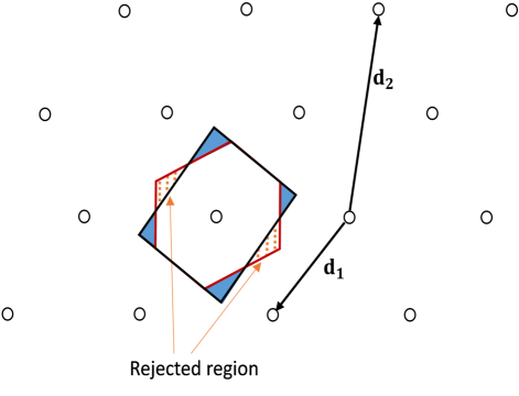
Figure 1: The rejected region (orange dots) of the possible projections $\pi_{\mathbf{D}_{\Gamma_{3}}}(\mathbf{d}_{3})$ in $\mathcal{L}(\mathbf{D}_{\Gamma_{3}})$ with respect to $\mathcal{V}_{\mathbf{0}}(\mathbf{D}_{\Gamma_{3}})$ (red hexagon) and $\mathcal{P}(\mathbf{d}_{1}^{*},\mathbf{d}_{2}^{*})$ (black rectangle), where the size reduction of LLL elongates $\mathbf{d}_{3}$. The four blue triangles are the region whose Babai point is the origin and size reductions cannot alter a suboptimal $\mathbf{d}_{3}$.

With the above demonstrations, we propose to amplify the success probabilities of Babai points with minimal efforts and to reject operations that elongate current basis vectors. Either using lattice Gaussian sampling [25] or PNP suffices the first objective, but we shall adhere to PNP because it is deterministic and this feature will be employed by (27). We detail the length reductions in boosted LLL as follows.

Assume we are working on the $\mathbf{R}$ matrix of a QR decomposition and trying to reduce $\mathbf{r}_{i}$ by $\mathbf{r}_{i-1},\ldots\thinspace,\mathbf{r}_{1}$. Let PNP be abstracted by a parameter $L=\prod_{k=1}^{i-1}p_{k}$ indicating the total number of routes it consists of, and $(p_{i-1},\ldots\thinspace,p_{1})\in(\mathbb{Z}^{+})^{i-1}$. Then each route of PNP can be marked by a label $(q_{i-1},\ldots\thinspace,q_{1})$ where $(q_{i-1},\ldots\thinspace,q_{1})\in\left\{1,\ldots\thinspace,p_{i-1}\right\}\times\cdots\times\left\{1,\ldots\thinspace,p_{1}\right\}$. From layer $i-1$ of each route, let $c_{i-1,(q_{i-1},...,q_{1})}$ be the $q_{i-1}$th closest integer to $\lfloor r_{i-1,i}/r_{i-1,i-1}\rceil$, and $\mathbf{r}_{i,(q_{i-1},...,q_{1})}=\mathbf{r}_{i}$, we set $\mathbf{r}_{i,(q_{i-1},...,q_{1})}\leftarrow\mathbf{r}_{i,(q_{i-1},...,q_{1})}-c_{i-1,(q_{i-1},...,q_{1})}\mathbf{r}_{i-1}$ and repeat this process down to layer $1$, resulting in $L$ pairs of coefficient vectors $\mathbf{c}_{(q_{i-1},...,q_{1})}=[-c_{1,(q_{i-1},...,q_{1})},\ldots\thinspace,-c_{i-1,(q_{i-1},...,q_{1})},1]$ and residuals $\mathbf{r}_{i,(q_{i-1},...,q_{1})}=\mathbf{R}_{\Gamma_{i+1}}\mathbf{c}_{(q_{i-1},...,q_{1})}$. We also mark the old $\mathbf{r}_{i}$ by $\mathbf{r}_{i,(0,\cdots,0)}=\mathbf{r}_{i}$, and $\mathbf{c}_{(0,\cdots,0)}=[0,\ldots\thinspace,0,1]$. At this stage, it can choose the shortest vector among all the $L+1$ candidates as the reduced version of $\mathbf{r}_{i}$, i.e., $\mathbf{r}_{i}=\mathbf{r}_{i,(z_{i-1}^{*},...,z_{1}^{*})}$ where

$$(z_{i-1}^{*},...,z_{1}^{*})=\arg\min_{(z_{i-1},...,z_{1})}\left\{\left\|\mathbf{r}_{i,(z_{i-1},...,z_{1})}\right\|\right\}.$$ (20)

If one also intends to export the unimodular transformation matrix $\mathbf{T}$, then it can be simultaneously updated inside PNP, which means $\mathbf{t}_{i,(z_{i-1}^{*},...,z_{1}^{*})}=\mathbf{T}_{\Gamma_{i+1}}\mathbf{c}_{(z_{i-1}^{*},...,z_{1}^{*})}$, $\mathbf{T}_{1:n,1:i}=\mathbf{t}_{i,(z_{i-1}^{*},...,z_{1}^{*})}$.

Since $|r_{k,i}/r_{k,k}|<1/2$ for $k<i$ is no longer guaranteed, together with the Lov sz condition they may destroy the Siegel condition [22] $r_{i-1,i-1}^{2}\leq(\frac{4}{3}+\varepsilon)r_{i,i}^{2}$ for $2\leq i\leq n$ with some small $\varepsilon>0$. For this reason, we should relax the Lov sz condition to the diagonal reduction (DR) condition [13].

Definition 6 (DR condition [13]).

An upper triangular lattice basis $\mathbf{R}$ satisfies the DR condition with parameter $\delta\thinspace(1/2<\delta<1)$ if it has

$$\delta r_{i-1,i-1}^{2}\leq r_{i,i}^{2}+(r_{i-1,i}-\lfloor r_{i-1,i}/r_{i-1,i-1}\rceil r_{i-1,i-1})^{2}$$ (21)

for all $2\leq i\leq n$, where $\delta$ is still referred to as the Lov sz constant.

If (21) holds, the Siegel condition must be true, so we let $i\leftarrow i+1$ and safely go to the next iteration. However, if (21) fails, one should also investigate whether a swap can tweak such cases. Consider the sublattice $\mathcal{L}(\mathbf{R}_{\Gamma_{i+1}})$ generated by the first $i$ vectors and define the potential of basis $\mathbf{R}$ [11] as

$$\mathrm{Pot}(\mathbf{R})=\prod_{i=1}^{n}\mathrm{det}(\mathcal{L}(\mathbf{R}_{\Gamma_{i+1}}))^{2}=\prod_{i=1}^{n}r_{i,i}^{2(n-i+1)}.$$ (22)

If the DR condition fails in $\pi_{\mathbf{R}_{\Gamma_{i}}}^{\perp}(\mathbf{R}_{1:n,i-1:i})$ and we swap $\mathbf{r}_{i-1}$ and $\mathbf{r}_{i}$, then the potential of the basis should be decreasing for the sake of bounding the number of iterations. After the swap, $\mathbf{R}_{i-1:i,i-1:i}$ becomes

$$\left[\begin{array}[]{cc}r_{i-1,i}&r_{i-1,i-1}\\ r_{i,i}&0\end{array}\right].$$ (23)

Let $\mathbf{G}$ be a $2\times 2$ unitary matrix

$$\left[\begin{array}[]{cc}\frac{r_{i-1,i}}{\sqrt{r_{i,i}^{2}+r_{i-1,i}^{2}}}&\frac{r_{i,i}}{\sqrt{r_{i,i}^{2}+r_{i-1,i}^{2}}}\\ -\frac{r_{i,i}}{\sqrt{r_{i,i}^{2}+r_{i-1,i}^{2}}}&\frac{r_{i-1,i}}{\sqrt{r_{i,i}^{2}+r_{i-1,i}^{2}}}\end{array}\right];$$ (24)

clearly, $\mathbf{G}\mathbf{R}_{i-1:i,1:n}$ can restore the upper triangular property of (23), which transforms to

$$\left[\begin{array}[]{cc}\sqrt{r_{i,i}^{2}+r_{i-1,i}^{2}}&\frac{r_{i-1,i}r_{i-1,i-1}}{\sqrt{r_{i,i}^{2}+r_{i-1,i}^{2}}}\\ 0&-\frac{r_{i,i}r_{i-1,i-1}}{\sqrt{r_{i,i}^{2}+r_{i-1,i}^{2}}}\end{array}\right].$$ (25)

From (22) and (25), one can obtain the potential ratio between two consecutive bases $\mathbf{R}^{\prime}$ and $\mathbf{R}$ as

$$\frac{\mathrm{Pot}(\mathbf{R}^{\prime})}{\mathrm{Pot}(\mathbf{R})} =\frac{\Big{(}\sqrt{r_{i,i}^{2}+r_{i-1,i}^{2}}\Big{)}^{2(n-i+2)}\Big{(}\frac{r_{i,i}r_{i-1,i-1}}{\sqrt{r_{i,i}^{2}+r_{i-1,i}^{2}}}\Big{)}^{2(n-i+1)}}{r_{i-1,i-1}^{2(n-i+2)}r_{i,i}^{2(n-i+1)}}$$

$$\leq\frac{\delta(r_{i,i}^{2}+r_{i-1,i}^{2})}{r_{i,i}^{2}+(r_{i-1,i}-\lfloor r_{i-1,i}/r_{i-1,i-1}\rceil r_{i-1,i-1})^{2}},$$ (26)

where the last inequality comes from (21). Based on (26), $\frac{\mathrm{Pot}(\mathbf{R}^{\prime})}{\mathrm{Pot}(\mathbf{R})}\leq\delta$ if and only if $\lfloor r_{i-1,i}/r_{i-1,i-1}\rceil=0$. As a result, preparing the pairs $\mathbf{t}_{i,(z_{i-1}^{*},...,z_{1}^{*})}$ and $\mathbf{r}_{i,(z_{i-1}^{*},...,z_{1}^{*})}$ based on (20) is only suitable for reductions before checking the DR conditions. In case that this condition fails, we should also prepare $\mathbf{t}_{i,(z_{i-1}^{{}^{\prime}},...,z_{1}^{{}^{\prime}})}$ and $\mathbf{r}_{i,(z_{i-1}^{{}^{\prime}},...,z_{1}^{{}^{\prime}})}$ that make $\lfloor r_{i-1,i}/r_{i-1,i-1}\rceil=0$:

$$(z_{i-1}^{{}^{\prime}},...,z_{1}^{{}^{\prime}})=\arg\min_{(z_{i-1},...,z_{1})}\Big{\{}\left\|\mathbf{r}_{i,(z_{i-1},...,z_{1})}\right\|,\thinspace\\ \mathrm{s.t.\thinspace}\lfloor r_{i-1,i,(z_{i-1},...,z_{1})}/r_{i-1,i-1}\rceil=0\thinspace\Big{\}},$$ (27)

in which $r_{i-1,i,(z_{i-1},...,z_{1})}$ denotes the $(i-1)$th component of $\mathbf{r}_{i,(z_{i-1},...,z_{1})}$. In such a manner, if a vector is swapped to the front, it is not only a short vector, but also the one that decreases the basis potential so that this kind of swaps cannot happen too many times.

IV-B Algorithm description

Combing the length reduction process above, the procedure of boosted LLL is given in Algorithm 2. Inside the loops, it employs a fixed structure column traverse strategy rather than using a parallel traversing [12, 13], such that a theoretical $O(n)$ factor in bounding the number of loops can be saved. In line 4, the PNP algorithm and rejection prepare two versions of reduced vectors. The stronger version $\mathbf{r}_{i,(z_{i-1}^{*},...,z_{1}^{*})}$ is used before testing the DR condition (line 6), so that the new $\mathbf{r}_{i}$ is the shortest candidate among the $L$ routes of PNP and the old $\mathbf{r}_{i}$. If it cannot pass this test, a weaker version $\mathbf{r}_{i,(z_{i-1}^{{}^{\prime}},...,z_{1}^{{}^{\prime}})}$ is used in line 7, who has identical value in the first layer as the Babai point and a variety of $p_{i-2}\times\cdots\times p_{1}$ routes in the remaining layers. Lastly, line 10 restores the upper triangular feature of $\mathbf{R}$ via a lightweight $2\times 2$ Givens rotation matrix and line 11 balances the unitary matrix. The toy example below may help to understand our algorithm.

Example 1.

Suppose we are reducing a matrix

$$\mathbf{R}=\left[\begin{array}[]{ccc}1&0.4&0\\ 0&1&0.52\\ 0&0&1\end{array}\right]$$

in round $i=3$ and executing from Line 4 of Algorithm 2. For the PNP algorithm, we set the $L=3$ routes as $p_{2}\times p_{1}=3\times 1$. The three nearest integers to $r_{2,3}/r_{2,2}$ are $1$, $0$, $2$, so the corresponding PNP routes are

$$\begin{cases}\mathbf{r}_{3,(1,1)}&=[-0.4,\thinspace-0.48,\thinspace 1]^{\top},\\ \mathbf{r}_{3,(2,1)}&=[0,\thinspace 0.52,\thinspace 1]^{\top},\\ \mathbf{r}_{3,(3,1)}&=[-0.8,\thinspace-1.48,\thinspace 1]^{\top},\end{cases}$$

and the rejection operation marking $\mathbf{r}_{3}$ is $\mathbf{r}_{3,(0,0)}=[0,\thinspace 0.52,\thinspace 1]^{\top}$. Eq. (20) would choose the shortest among the above four routes. Let it be $\mathbf{r}_{3,(2,1)}$ (or $\mathbf{r}_{3,(0,0)}$), which is employed by Line 5. Eq. (27) can only choose from $\mathbf{r}_{3,(1,1)}$. Then we test the DR condition and it succeeds, so the while loop stops.

Input: original lattice basis $\mathbf{D}\in\mathbb{R}^{n\times n}$, Lov sz constant $\delta$, list number $L$.

Output: reduced basis $\mathbf{D}$, unimodular matrix $\mathbf{T}$

1 $[\mathbf{Q},\mathbf{R}]=\mathrm{qr}(\mathbf{D})$; $\triangleright$ The QR decomposition of $\mathbf{D}$;

2 $i=2$, $\mathbf{T}=\mathbf{I}$;

3 while $i\leq n$ do

4       use (20) to get $[\mathbf{r}_{i,(z_{i-1}^{*},...,z_{1}^{*})},\mathbf{t}_{i,(z_{i-1}^{*},...,z_{1}^{*})}]$ and use (27) to get $[\mathbf{r}_{i,(z_{i-1}^{{}^{\prime}},...,z_{1}^{{}^{\prime}})},\mathbf{t}_{i,(z_{i-1}^{{}^{\prime}},...,z_{1}^{{}^{\prime}})}]$;

5       $\mathbf{R}_{1:n,i}=\mathbf{r}_{i,(z_{i-1}^{*},...,z_{1}^{*})}$,$\mathbf{T}_{1:n,i}=\mathbf{t}_{i,(z_{i-1}^{*},...,z_{1}^{*})}$;

6       if condition (21) fails then

7             $\mathbf{R}_{1:n,i}=\mathbf{r}_{i,(z_{i-1}^{{}^{\prime}},...,z_{1}^{{}^{\prime}})}$,$\mathbf{T}_{1:n,i}=\mathbf{t}_{i,(z_{i-1}^{{}^{\prime}},...,z_{1}^{{}^{\prime}})}$;

8             define $\mathbf{G}$ as in (24);

9             swap $\mathbf{R}_{1:n,i}$ and $\mathbf{R}_{1:n,i-1}$, $\mathbf{T}_{1:n,i}$ and $\mathbf{T}_{1:n,i-1}$ ;

10             $\mathbf{R}_{i-1:i,1:n}\leftarrow\mathbf{G}\mathbf{R}_{i-1:i,1:n}$;

11             $\mathbf{Q}_{1:n,i-1:i}\leftarrow\mathbf{Q}_{1:n,i-1:i}\mathbf{G}^{\top}$;

12             $i\leftarrow\max(i-1,2)$;

13      else

14             $i\leftarrow i+1$;

15      

$\mathbf{D}\leftarrow\mathbf{Q}\mathbf{R}.$

Algorithm 2 The boosted LLL algorithm.

In essence, this algorithm attempts to minimize the basis length while keeping the Siegel condition, and the PNP algorithm offers flexible efforts to do so. If we replace lines 4 and 5 by using the Babai point and delete line 7, Algorithm 2 degrades to the classic LLL algorithm [11].

IV-C Properties of boosted LLL

When the boosted LLL algorithm terminates, $\delta r_{i-1,i-1}^{2}-(\frac{r_{i-1,i}}{r_{i-1,i-1}}-\lfloor\frac{r_{i-1,i}}{r_{i-1,i-1}}\rceil)^{2}r_{i-1,i-1}^{2}\leq r_{i,i}^{2}$ holds for all $2\leq i\leq n$, which ensure the Siegel properties hold:

$$|r_{i-1,i-1}|\leq\beta|r_{i,i}|.$$ (28)

Assume the PNP algorithm has parameters $(p_{k-1},\ldots\thinspace,p_{1})$ for $2\leq k\leq n$, then $\pi_{\mathbf{R}_{\Gamma_{i}}}(\mathbf{r}_{i})$ is contained in $\mathcal{V}_{\mathbf{0}}(\mathbf{R}_{\Gamma_{i}})\cup\mathcal{P}(\left[q_{1}\mathbf{r}_{1}^{*},\ldots\thinspace,q_{i-1}\mathbf{r}_{i-1}^{*}\right])$, where $\left\{\mathbf{r}_{1}^{*},\ldots\thinspace,\mathbf{r}_{i-1}^{*}\right\}$ are the GSO vectors of $\mathbf{R}_{\Gamma_{i}}$. Though this region can be much larger than $\mathcal{P}(\left[\mathbf{r}_{1}^{*},\ldots\thinspace,\mathbf{r}_{i-1}^{*}\right])$, we have

$$\left\|\mathbf{r}_{i}\right\|^{2}\leq r_{i,i}^{2}+\frac{1}{4}\sum_{j<i}r_{j,j}^{2}$$ (29)

if $\pi_{\mathbf{R}_{\Gamma_{i}}}(\mathbf{r}_{i})\in\mathcal{P}(\left[\mathbf{r}_{1}^{*},\ldots\thinspace,\mathbf{r}_{i-1}^{*}\right])$. If $\pi_{\mathbf{R}_{\Gamma_{i}}}(\mathbf{r}_{i})\notin\mathcal{P}(\left[\mathbf{r}_{1}^{*},\ldots\thinspace,\mathbf{r}_{i-1}^{*}\right])$, we can always find the Babai point $\mathbf{r}_{i}^{\prime}$ such that $\left\|\mathbf{r}_{i}\right\|^{2}<\left\|\mathbf{r}_{i}^{\prime}\right\|^{2}\leq r_{i,i}^{2}+\frac{1}{4}\sum_{j<i}r_{j,j}^{2}$ due to (20) and (27), so condition (29) always holds in boosted LLL.

With (28) and (29), classical properties of LLL can be trivially proved:

$$l(\mathbf{D})\leq\beta^{n-1}\lambda_{n}(\mathbf{D}),$$ (30)

$$\xi(\mathbf{D})\leq\beta^{n(n-1)/2}.$$ (31)

Since we have devoted much effort to implement the length reductions, (30) and (31) are the least bounds that we should expect from boosted LLL. However, moving any step forward seems difficult because even using CVP as length reduction still fails to generate a better explicit bound than (29). The difficulty of improving bounds on lengths exists in all variants of LLL, including the LLL with deep insertions (LLL-deep) [18]. In this regard, boosted LLL only serves as an ameliorated practical algorithm.

IV-D Implementation and Complexity

The total number of loops $K$ in Algorithm 2 equals to the number testing condition (21), whose number of positive and negative tests are denoted as $K^{+}$ and $K^{-}$, respectively. The total number of negative test is

$$K^{-}\leq\log_{1/\delta}\frac{\mathrm{Pot}(\mathbf{D}_{0})}{\mathrm{Pot}(\mathbf{D}_{K})}=\frac{1}{\ln(1/\delta)}\times\ln\left(\frac{\mathrm{Pot}(\mathbf{D}_{0})}{\mathrm{Pot}(\mathbf{D}_{K})}\right),$$ (32)

where $\mathbf{D}_{0}$, $\mathbf{D}_{K}$ are the initial basis and the basis after $K$ loops, respectively. In the fixed traversing strategy, we also have $K^{+}\leq K^{-}+n-1$. We first show how to choose $\delta$ such that the boosted LLL algorithm has the best performance while $\frac{1}{\ln(1/\delta)}$ remains to be a polynomial number. After that, $\frac{\mathrm{Pot}(\mathbf{D}_{0})}{\mathrm{Pot}(\mathbf{D}_{K})}$ is evaluated to complete our complexity analysis.

IV-D1 Optimal $\delta$

Among literature, $\delta$ is often chosen arbitrarily close to $1$ while explanations are lacking. In Micciancio’s book [1, Lem. 2.9], it is shown if $\delta=1/4+(3/4)^{n/(n-1)}$, then $\frac{1}{\ln(1/\delta)}\leq n^{c}$ for all $c>1$. More generally, we can define an optimal principle of choosing $\delta$, i.e.,

$$\delta(a^{*},n)=\frac{1}{a^{*}}+\left(\frac{a^{*}-1}{a^{*}}\right)^{n/(n-1)}$$

where $a^{*}=\frac{1}{1-e^{-1}}$.

With such settings, three distinctive properties exist: $\frac{1}{\ln(1/\delta)}\leq n^{c}$ for all $n$; $\delta$ is asymptotically close to $1$ so that the algorithm has the best performance; and it is the smallest value satisfying the previous two attributes (the fastest one among the class of best performance). Proposition 6 justifies these claims and the proof is given in Appendix E.

Proposition 6.

For arbitrary constants $a>1$, $c>1$, if $\delta(a,\thinspace n)=\frac{1}{a}+\left(\frac{a-1}{a}\right)^{n/(n-1)}$, then for all $n$,

$$\frac{1}{\ln(1/\delta)}\leq n^{c}.$$ (33)

Let $a^{*}=\lim_{n\rightarrow\infty}\arg\min_{a}\delta(a,\thinspace n)$ be defined as the universal good constant, then

$$a^{*}=\frac{1}{1-e^{-1}}.$$ (34)

IV-D2 Total complexity in flops

Further define $\psi(\mathbf{D})=\min_{i}r_{i,i}^{2}$ and $\Psi(\mathbf{D})=\max_{i}r_{i,i}^{2}$. Since our length reduction does not change $r_{i,i}$ while (25) shows that any swap can narrow the gap between $r_{i-1,i-1}$ and $r_{i,i}$, the number of negative tests between the initial basis $\mathbf{D}_{0}$ to the final basis $\mathbf{D}_{K}$ is

$$K^{-} \leq n^{c}\ln\left(\frac{\mathrm{Pot}(\mathbf{D}_{0})}{\mathrm{Pot}(\mathbf{D}_{K})}\right)$$

$$\leq\frac{n^{c+1}(n+1)}{2}\ln\left(\frac{\Psi(\mathbf{D}_{0})}{\psi(\mathbf{D}_{0})}\right).$$ (35)

With reference to [36], we have $\frac{\Psi(\mathbf{D}_{0})}{\psi(\mathbf{D}_{0})}\leq\kappa(\mathbf{D}_{0})$, where $\kappa(\mathbf{D}_{0})$ is the condition number of $\mathbf{D}_{0}$. So if the condition number of the input basis satisfies $\ln\kappa(\mathbf{D}_{0})=O(\ln n)$, then the number of iterations in boosted LLL is $K\leq 2K^{-}+n-1=O(n^{c+2}\ln n)$, where $c>1$ is a constant arbitrarily close to $1$. By further counting the number of flops inside and outside the loop of Algorithm 2, the total complexity of boosted LLL is $O(Ln^{4+c}\ln n)$.

Remark 3.

The complexity analysis above is quite general. For instance, if $\mathbf{D}_{0}$ is Gaussian, then it follows from [36] that $\mathbb{E}(\ln\kappa(\mathbf{D}_{0}))\leq\ln n+2.24$. In the application to IF [21], we can also take a detour to employ this property of Gaussian matrices. Firstly, the condition number of the input basis $\mathbf{D}_{0}$ would increase if the signal to noise ratio (SNR) rises, so it suffices to investigate the case for infinite SNR. The target then becomes the dual of a Gaussian random matrix that has the same condition number, so $\mathbb{E}(\ln\kappa(\mathbf{D}_{0}))\leq\ln n+2.24$ also holds in IF.

V Application to integer forcing

In the context of optimizing the achievable rates of IF, some results based on LR have been presented in [37], where the difference between KZ and Minkowski is not obvious because the system size is small ($2\times 2$ or $4\times 4$). Since we have improved the classic KZ and LLL, we will verify our boosted algorithms in IF by showing their performance about ergodic rates, orthogonal defects (inversely proportional to sum-rates), and complexity in flops.

V-A IF and SBP

In this subsection, the IF transceiver architecture will be reviewed by using real value representations for simplicity. In a MIMO system with size $n\times n$, each antenna has a message

$$\mathbf{w}_{i}=[w_{i}(1),w_{i}(2),\ldots\thinspace,w_{i}(k)]^{\top},$$

where $i\in\left\{1,\ldots\thinspace,n\right\}$, $\mathbf{w}_{i}\in\mathbb{F}_{p}^{k}$, and $\mathbb{F}_{p}$ is a finite field with size $p$. As the conversion from message layer to physical layer, an encoder $\mathcal{E}_{i}:\thinspace\mathbb{F}_{p}^{k}\rightarrow\mathbb{R}^{n}$ maps the length-$k$ message $\mathbf{w}_{i}$ into a lattice codeword

$$\mathbf{x}_{i}=[x_{i}(1),x_{i}(2),\ldots\thinspace,x_{i}(T)]^{\top},$$

where $\left\|\mathbf{x}_{i}\right\|^{2}\leq TP$, $T$ stands for code length and $P$ stands for SNR. All encoders operate at the same lattice with the same rate:

$$R_{\mathrm{TX}}=\frac{k}{T}\log_{2}p.$$

Let $x_{i}(j)$ be the $j$th symbol of $\mathbf{x}_{i}$, we may write the transmitted vector across all antennas in time $j$ as $\mathbf{x}[j]=[x_{1}(j),\ldots\thinspace,x_{n}(j)]^{\top}$. An observation $\mathbf{y}[j]\in\mathbb{R}^{n}$ can be subsequently written as

$$\mathbf{y}[j]=\mathbf{H}\mathbf{x}[j]+\mathbf{z}[j]$$ (36)

in which $\mathbf{H}\in\mathbb{R}^{n\times n}$ denotes the MIMO channel matrix and $\mathbf{z}[j]$ is the additive white Gaussian noise (AWGN) with $z_{i}[j]\sim\mathcal{N}(0,1)$. Let $\mathbf{Y}$, $\mathbf{X}$, and $\mathbf{Z}$ be the concatenated $\mathbf{y}[j]$, $\mathbf{x}[j]$ and $\mathbf{z}[j]$ from time slots $1$ to $T$. In a linear receiver architecture, the receiver will project $\mathbf{Y}$ with a matrix $\mathbf{B}=[\mathbf{b}_{1},\ldots\thinspace,\mathbf{b}_{n}]^{\top}\in\mathbb{R}^{n\times n}$ to get the useful information $\mathbf{A}\mathbf{X}$ for further decoding,

$$\mathbf{B}\mathbf{Y}=\underset{\mathrm{useful\thinspace information}}{\underbrace{\mathbf{A}\mathbf{X}}}+\underset{\mathrm{effective\thinspace noise}}{\underbrace{(\mathbf{B}\mathbf{H}-\mathbf{A})\mathbf{X}+\mathbf{B}\mathbf{Z}}}.$$ (37)

We choose $\mathbf{A}=[\mathbf{a}_{1},\ldots\thinspace,\mathbf{a}_{n}]^{\top}\in\mathbb{Z}^{n\times n}$ because these lattice codewords are closed under integer combinations. $\mathbf{A}$ should also be full rank to avoid losing information.

For a preprocessing matrix $\mathbf{B}$, the following computation rate can be obtained in the $i$th effective channel if the coding lattices satisfy goodnesses for channel coding and quantization [21]

$$R(\mathbf{H},\mathbf{a}_{i},\mathbf{b}_{i})=\frac{1}{2}\log_{2}^{+}\left(\frac{P}{\left\|\mathbf{b}_{i}\right\|^{2}+P\left\|\mathbf{H}^{\top}\mathbf{b}_{i}-\mathbf{a}_{i}\right\|^{2}}\right),$$ (38)

where $\mathrm{log}_{2}^{+}(x)=\max\left\{\log_{2}(x),0\right\}$.

The first step towards maximizing the rates is to set $\partial\left\{\left\|\mathbf{b}_{i}\right\|^{2}+P\left\|\mathbf{H}^{\top}\mathbf{b}_{i}-\mathbf{a}_{i}\right\|^{2}\right\}/\partial\mathbf{b}_{i}=\mathbf{0}$ for a fixed IF coefficient matrix $\mathbf{A}$, which leads to

$$\mathbf{b}_{i}=(\mathbf{H}\mathbf{H}^{\top}+\frac{1}{P}\mathbf{I})^{-1}\mathbf{H}\mathbf{a}_{i}.$$

Plug this into (38) and use Woodbury matrix identity for the inverse of a matrix, we have

$$R(\mathbf{H},\mathbf{a}_{i}) = \frac{1}{2}\log_{2}^{+}\left(\frac{P}{\left\|\mathbf{D}\mathbf{a}_{i}\right\|^{2}}\right),$$ (39)

where $\mathbf{D}=\Lambda^{-\frac{1}{2}}\mathbf{V}^{\top}$ and $\mathbf{V}\Lambda\mathbf{V}^{\top}=\mathbf{H}^{\top}\mathbf{H}+1/P\mathbf{I}$ is the eigendecomposition. Achieving the optimum rate is therefore equivalent to solving SIVP on lattice $\mathcal{L}(\mathbf{D})$:

$$\arg\min_{\mathbf{A}\in\mathbb{Z}^{n\times n},\thinspace\mathrm{rank}(\mathbf{A})=n}\max_{i}\left\|\mathbf{D}\mathbf{a}_{i}\right\|^{2},$$ (40)

in which $\min_{\mathbf{A}\in\mathbb{Z}^{n\times n},\thinspace\mathrm{rank}(\mathbf{A})=n}\max_{i}\left\|\mathbf{D}\mathbf{a}_{i}\right\|^{2}=\lambda_{n}(\mathbf{D})$.

Now we explain how to obtain the estimations of messages. Upon quantizing $\mathbf{\mathbf{B}\mathbf{Y}}$ to the fine lattice and modulo the coarse lattice in a row-wise manner [23], a converter $\mathcal{D}_{i}:\thinspace\mathbb{R}^{n}\rightarrow\mathbb{F}_{p}^{k}$ then maps the physical layer codeword to a message under finite field representations, i.e., $\hat{\mathbf{u}}_{i}=[\mathbf{W}^{\top}\mathbf{a}_{i}]\thinspace\mod\thinspace p$, $\mathbf{W}=[\mathbf{w}_{1},\ldots\thinspace,\mathbf{w}_{n}]^{\top}$. These combinations are then collected, so as to decode the messages as

$$\left[\hat{\mathbf{w}}_{1},\ldots\thinspace,\hat{\mathbf{w}}_{n}\right]^{\top}=\mathbf{A}_{p}^{-1}\left[\hat{\mathbf{u}}_{1},\ldots\thinspace,\hat{\mathbf{u}}_{n}\right]^{\top},$$

where $\mathbf{A}_{p}$ is a full rank matrix over $\mathbb{Z}_{p}$ and $\mathbf{A}_{p}^{-1}$ is taken over the same field.

With the above demonstrations in mind, there should be at least two reasons for us to restrain SIVP to SBP

$$\arg\min_{\mathbf{A}\in\mathrm{GL}_{n}(\mathbb{Z})}\max_{i}\left\|\mathbf{D}\mathbf{a}_{i}\right\|^{2}.$$ (41)

The first reason is about flexibility. With SBP, we can choose among lattice reduction algorithms from polynomial to exponential complexity with guaranteed properties, and these algorithms are still efficient when SNR is high. The second reason is about complexity, where the inverse of $\mathbf{A}$ over finite fields is much easier to calculate when $\mathbf{A}\in\mathrm{GL}_{n}(\mathbb{Z})$, and algorithms for SIVP or the successive minima problem (SMP) are generally more complicated than those of SBP [37, 38]. For instance, we can observe that for the enumeration routines of SMP, Minkowski reduction and boosted KZ reduction, one needs to verify the linear independence of a new vector with previous lattice vectors for SMP, while Minkowski reduction only needs to check the greatest common divisor of the enumerated coefficients [10] and boosted KZ does not require such inspections.

V-B Simulation results

This subsection examines the rates and complexity performance when applying the proposed boosted KZ and boosted LLL algorithms for IF receivers. We show the achievable rates rather than the bit error rates of IF MIMO receivers, since the latter depend on which capacity-approaching code for the AWGN channel is used at the transmitter. All simulations are performed on real matrices with random entries drawn from i.i.d. Gaussian distributions $\mathcal{N}(0,1)$. Results in the figures are all averaged from $10^{3}$ Monte Carlo runs.

The boosted LLL algorithm is referred as “b-LLL-$L$” with $L$ being the total number of branches in the PNP algorithm, i.e., $L=p_{i-1}p_{i-2}\cdots p_{1}$ remains unchanged for different columns $i$’s. If $L=1$, this version means only adding a rejection operation to the classic LLL algorithm [11]. When $L=3$ or $L=9$, we expand $3$ branches in the first or first two layers of the PNP algorithm. Regarding other typical variants of LLL, such as the effective LLL [12] and greedy LLL [17], they all boil down to the same performance as LLL if we implement a full size reduction at the end of their algorithms, so we omit comparing our algorithms with these variants.

The boosted KZ algorithm (“b-KZ”) is implemented as described in Algorithm 1. To ensure a fair comparison, the KZ algorithm follows the same routine as Algorithm 1 except replacing the “CVP subroutine” with a size reduction. Minkowski reduction is also included as our reference with the label “Minkow”, whose implementation follows [10, Sec. V].

V-B1 Achievable rate

The actual achievable rate of the IF receivers can be quantitatively evaluated by the ergodic rate defined by [37]

$$R_{E}=\mathbb{E}\Big{(}n\min_{i}R(\mathbf{H},\mathbf{a}_{i})\Big{)},$$

where the expectation is taken over different realizations of $\mathbf{H}$, and $R(\mathbf{H},\mathbf{a}_{i})$ was defined in (39).

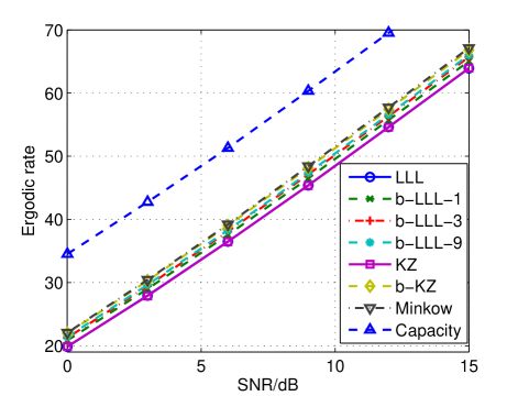
Figure 2: SNR versus ergodic rate for different LR algorithms.

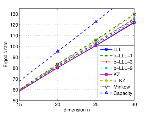
Figure 3: Dimension versus ergodic rate for different LR algorithms.

In Fig. 2, we have plotted the rate performance of different LR algorithms in a $20\times 20$ real-valued MIMO channel, in which the channel capacity $\frac{1}{2}\log_{2}(\det(\mathbf{I}+P\mathbf{H}\mathbf{H}^{\top}))$ serves as an upper bound. In the figure, the b-LLL-1 algorithm has higher rates than KZ and LLL, and the improvements after we increase the list number to $L=3,\thinspace 9$ can still be spotted in this crowded figure. The b-KZ method attains almost the same rates as those of Minkowski reduction. KZ reduction does not offer better rates than LLL because KZ only guarantees to yield a basis with the smallest potential, and both of them are under the curse Proposition 1.

In Fig. 3, we fixed the SNR to be $20\mathrm{dB}$ and study how the size of the system is affecting their ergodic rates. From this graph, the differences of rates among different LR methods amplify as dimension $n$ increases, and their mutual relations are the same as those of Fig. 2.

V-B2 Orthogonal defect

The ergodic rate $R_{E}$ is only determined by the basis length $l(\mathbf{D})$. To evaluate the sum-rates for all data streams, OD’s can be employed which are proportional to the length products of basis vectors. Such a quantity can reveal the gaps between different algorithms more vividly.

Figure 4: SNR versus OD for different LR algorithms.

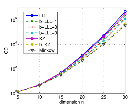
Figure 5: Dimension versus OD for different LR algorithms.

In Figs. 4 (fixed size of $20\times 20$) and 5 (fixed SNR of $20\mathrm{dB}$), we have plotted the SNR versus OD, and dimension versus OD relations for distinct lattice reduction algorithms. From these two figures, several phenomenons can be observed. Boosted KZ cannot surpass Minkowski reduction but remains close to it. The performance improvements from b-LLL-$1$, to b-LLL-$3$, b-LLL-$9$ are approximately proportional to the increment in the list size $L$. One interesting thing to observe from Fig. 4 is, the performance gaps between boosted and non-boosted algorithms are becoming larger as $P$ rises. Since $\mathbf{D}=\Lambda^{-\frac{1}{2}}\mathbf{V}^{\top}$ and $\mathbf{V}\Lambda\mathbf{V}^{\top}=\mathbf{H}^{\top}\mathbf{H}+1/P\mathbf{I}$, the increment of $P$ is, intrinsically, changing the goodness of the corresponding minimal basis. It also says that the possibility of size reduction being suboptimal would increase if the lattice bases tend to be more random. Lastly, Fig. 5 shows an evident “Minkow < b-KZ < b-LLL-9 < b-LLL-3 < b-LLL-1 < KZ < LLL” relation about OD, and their OD values are much better than their theoretical bounds (see e.g., Eqs. (13) and (31)).

V-B3 Complexity

In addition to our theoretical analysis on the complexity of the proposed algorithms, we further compare their empirical costs by the expected number of flops, which are clearly shown in Fig. 6. Not surprisingly, the b-KZ algorithm spends about $1.5$ times the efforts of KZ in the dimensions depicted in Fig. 6, and the b-LLL-1, 3, 9 algorithms costs around $1,\thinspace 1.5,$ and $3$ times the efforts of LLL. Both b-KZ and KZ reductions have dramatically lower number of flops than Minkowski reduction. Moreover, the boosted LLL algorithms have much smaller complexity than KZ while reducing the bases more effectively as Figs. 2 to 5 have revealed.

To sum up, concerning the complexity-performance tradeoffs as well as the theoretical bounds, the boosted KZ and LLL algorithms can be the ideal candidates for reducing lattice bases in IF with exponential and polynomial complexity, respectively.

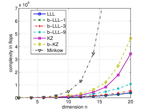
Figure 6: Dimension versus complexity for different LR algorithms.

VI Open questions

We have only demonstrated the theoretical superiority of boosted KZ over KZ and Minkowski, while Minkowski reduction still yields shorter vectors in our simulations. One interesting open question is whether there exist better performance bounds for Minkowski reduction. It is also of sufficient interests to improve the performance analysis on boosted LLL.

Appendix A Proof of proposition 2

Proof:

First of all, the reducible condition $\left\|\mathbf{d}_{i}-\mathbf{v}\right\|^{2}<\left\|\mathbf{d}_{i}\right\|^{2}$ can be reformulated as $\left\|\pi_{\mathbf{D}_{\Gamma_{i}}}(\mathbf{d}_{i})-\mathbf{v}\right\|^{2}<\left\|\pi_{\mathbf{D}_{\Gamma_{i}}}(\mathbf{d}_{i})\right\|^{2}$, which becomes equivalent to

$$\left\|\mathbf{v}\right\|^{2}/2<\langle\pi_{\mathbf{D}_{\Gamma_{i}}}(\mathbf{d}_{i}),\mathbf{v}\rangle.$$ (42)

It is necessary to show $\langle\pi_{\mathbf{D}_{\Gamma_{i}}}(\mathbf{d}_{i}),\mathbf{v}\rangle>0$ for $\mathbf{v}\neq\mathbf{0}$ so that the inequality we pursuit makes sense. We give a proof by contradiction. Suppose that $\theta(\pi_{\mathbf{D}_{\Gamma_{i}}}(\mathbf{d}_{i}),\mathbf{v})>\pi/2$, due to symmetricity of the Voronoi cell $\mathcal{V}_{\mathbf{v}}(\mathbf{D}_{\Gamma_{i}})$, there exists a symmetric point $\mathbf{d}_{i}^{\prime}$ of $\pi_{\mathbf{D}_{\Gamma_{i}}}(\mathbf{d}_{i})$ on $\mathbf{v}$, such that $\theta(\mathbf{d}_{i}^{\prime},\mathbf{v})>\pi/2$. Define the half-space of $\mathbf{v}$ as $\mathcal{H}_{\mathbf{v}}=\left\{\mathbf{x}\in\mathbb{R}^{n}\mid\langle\mathbf{v},\mathbf{x}\rangle>0\right\}$, then the convex combination among $\left\{\mathcal{V}_{\mathbf{v}}(\mathbf{D}_{\Gamma_{i}})\cap\mathcal{H}_{\mathbf{v}},\pi_{\mathbf{D}_{\Gamma_{i}}}(\mathbf{d}_{i}),\mathbf{d}_{i}^{\prime}\right\}$ must include the origin. Then there are two lattice points ($\mathbf{0}$ and $\mathbf{v}$) inside $\mathcal{V}_{\mathbf{v}}(\mathbf{D}_{\Gamma_{i}})$, which contradicts the basic property of a Voronoi cell, i.e., there can be only one lattice point inside a Voronoi region.

We proceed to prove (42). Since $\pi_{\mathbf{D}_{\Gamma_{i}}}(\mathbf{d}_{i})$ is quantized to $\mathbf{v}$, their difference $\pi_{\mathbf{D}_{\Gamma_{i}}}(\mathbf{d}_{i})-\mathbf{v}$ lies inside the Voronoi cell $\mathcal{V}_{\mathbf{0}}(\mathbf{D}_{\Gamma_{i}})$, which yields $\langle\pi_{\mathbf{D}_{\Gamma_{i}}}(\mathbf{d}_{i})-\mathbf{v},\mathbf{w}\rangle<\left\|\mathbf{w}\right\|^{2}/2$ for all $\mathbf{w}\in\mathcal{L}(\mathbf{D}_{\Gamma_{i}})$ and $\mathbf{w}\neq\mathbf{0}$. As $\mathbf{v}-\pi_{\mathbf{D}_{\Gamma_{i}}}(\mathbf{d}_{i})\in\mathcal{V}_{\mathbf{0}}(\mathbf{D}_{\Gamma_{i}})$, choose an instance of $\mathbf{w}=\mathbf{v}\neq\mathbf{0}$ for $\langle\mathbf{v}-\pi_{\mathbf{D}_{\Gamma_{i}}}(\mathbf{d}_{i}),\mathbf{w}\rangle<\left\|\mathbf{w}\right\|^{2}/2$, then (42) is obtained. ∎

Appendix B Proof of proposition 3

Proof:

Regarding (9), first recall a fact that we cannot produce $n$ independent vectors by using a lattice of rank $n-1$, then among $\lambda_{1}(\mathbf{D}),\ldots\thinspace,\lambda_{n}(\mathbf{D})$, at least one of them, e.g., $\lambda_{i^{\prime}}(\mathbf{D})$, corresponds to $\mathbf{v}=x_{n}\mathbf{d}_{n}+\sum_{i=1}^{n-1}x_{i}\mathbf{d}_{i}$ where $\sum_{i=1}^{n-1}x_{i}\mathbf{d}_{i}\in\mathcal{L}(\mathbf{D}_{\Gamma_{n}})$, $x_{n}\in\mathbb{Z}\setminus 0$. With QR decomposition $[\mathbf{Q},\mathbf{R}]=\mathrm{qr}(\mathbf{D})$,

$$\mathbf{v} = \sum_{i=1}^{n}x_{i}\left(r_{i,i}\mathbf{q}_{i}+\sum_{j=1}^{i-1}r_{j,i}\mathbf{q}_{j}\right)$$

$$= \sum_{i=1}^{n-1}x_{i}\left(r_{i,i}\mathbf{q}_{i}+\sum_{j=1}^{i-1}r_{j,i}\mathbf{q}_{j}\right)+x_{n}r_{n,n}\mathbf{q}_{n}.$$

Notice that $-\mathbf{v}$ also corresponds to $\lambda_{i^{\prime}}(\mathbf{D})$, so we can confine $x_{n}>0$ and consider the following two cases.

1) If $x_{n}>1$, it is observed that $\left\|\mathbf{v}\right\|=\left\|\sum_{i=1}^{n-1}x_{i}\left(r_{i,i}\mathbf{q}_{i}+\sum_{j=1}^{i-1}r_{j,i}\mathbf{q}_{j}\right)+x_{n}r_{n,n}\mathbf{q}_{n}\right\|\geq x_{n}|r_{n,n}|$ because the $\mathbf{q}_{i}$’s are orthogonal, which yields

$$|r_{n,n}|^{2}\leq\frac{1}{x_{n}^{2}}\lambda_{i^{\prime}}(\mathbf{D})^{2}\leq\frac{1}{4}\lambda_{n}(\mathbf{D})^{2}.$$ (43)

We then proceed to bound the last term in (7). For $1\leq i\leq n$, the covering radius of lattice $\mathcal{\mathcal{L}}(\mathbf{D}_{\Gamma_{n}})$ is

$$\rho(\mathbf{D}_{\Gamma_{n}}) = \max_{\mathbf{x}}\mathrm{dist}\left(\mathbf{x},\mathcal{L}(\mathbf{D}_{\Gamma_{n}})\right)$$ (44)

$$\leq 1/2\sqrt{\sum_{k=1}^{n-1}r_{k,k}^{2}},$$

where the inequality is obtained after choosing $\mathbf{x}$ as a “deep hole” [39, P. 33] and solving this CVP by applying Babai’s nearest plane algorithm [40]. Since boosted KZ still assures $|r_{k,k}|=\lambda_{1}(\pi_{\mathbf{D}_{\Gamma_{k}}}^{\perp}([\mathbf{d}_{k},\ldots\thinspace,\mathbf{d}_{n}]))$, and the projection of the $k$th successive minimum in $\mathbf{D}$ onto the orthogonal complement of $\mathbf{D}_{\Gamma_{k}}$ must have a least one non-zero coefficient for $[\mathbf{d}_{k},\ldots\thinspace,\mathbf{d}_{n}]$, we have $|r_{k,k}|\leq\lambda_{k}(\mathbf{D})$; plug this into (44),

$$\rho(\mathbf{D}_{\Gamma_{n}})\leq 1/2\sqrt{\sum_{k=1}^{n-1}\lambda_{k}(\mathbf{D})^{2}}.$$ (45)

Put (43) and (45) into (7), then $\left\|\mathbf{d}_{n}\right\|^{2}\leq\frac{1}{4}\lambda_{n}(\mathbf{D})^{2}+\frac{1}{4}\sum_{k=1}^{n-1}\lambda_{k}(\mathbf{D})^{2}\leq\frac{n}{4}\lambda_{n}(\mathbf{D})^{2}$.

2) If $x_{n}=1$, recall that our length reduction by CVP (line 11) ensures $\mathbf{d}_{n}$ is the shortest vector among the set $\left\{\mathbf{d}_{n}+\sum_{i=1}^{n-1}z_{i}\mathbf{d}_{i}\mid\forall\thinspace z_{i}\in\mathbb{Z}\right\}$, so $\left\|\mathbf{d}_{n}\right\|\leq\lambda_{i^{\prime}}(\mathbf{D})\leq\lambda_{n}(\mathbf{D})$ in such a scenario.

Combining 1) and 2) proves (9).

As for (8), since all sublattices $\left\{\mathcal{L}(\mathbf{D}_{\Gamma_{i+1}})\mid 1\leq i\leq n\right\}$ are also boosted KZ reduced, it follows from the proved (9) that $\left\|\mathbf{d}_{i}\right\|\leq\max\left\{1,\thinspace\frac{\sqrt{i}}{2}\right\}\lambda_{i}(\mathbf{D}_{\Gamma_{i+1}})$. With $|r_{i,i}|\leq\lambda_{i}(\mathbf{D})$ and the bound for the covering radius, we also have $\left\|\mathbf{d}_{i}\right\|\leq\frac{\sqrt{i+3}}{2}\lambda_{i}(\mathbf{D})$ for all $i$. So choosing the minimum among them yields (8). ∎

Appendix C Proof of proposition 4

Proof:

Since $|r_{i,i}|=\lambda_{1}(\mathbf{R}_{i:n,i:n})$, we apply Minkowski’s second theorem [31, P. 202] to lattices $\mathcal{L}(\mathbf{R}_{i:n,i:n})$ with $1\leq i\leq n-1$, then we have $r_{n-j+1,n-j+1}^{2}\leq\gamma_{j}\left(\prod_{k=1}^{j}r_{n-k+1,n-k+1}^{2}\right)^{1/j}$. As those of [28, Prop. 4.2], we cancel duplicated terms in this inequality and use induction from $\mathcal{L}(\mathbf{R}_{n-1:n,n-1:n})$ to $\mathcal{L}(\mathbf{R}_{1:n,1:n})$, then

$$r_{n-j+1,n-j+1}^{2}\leq\gamma_{j}\left(\prod_{k=2}^{j}\gamma_{k}^{1/(k-1)}\right)r_{n,n}^{2}.$$ (46)

As $\gamma_{j}\leq\frac{2j}{3}$, we define $g(j)=\frac{2j}{3}\prod_{k=2}^{j}\left(\frac{2k}{3}\right)^{1/(k-1)}$ and evaluate this term. Let $z=k-1$, it can be shown that

$$g(j) = \frac{8j}{9}\exp\left(\sum_{z=2}^{j-1}\ln\left(\frac{2z+2}{3}\right)\frac{1}{z}\right)$$

$$\overset{(a)}{\leq} \frac{8j}{9}\exp\left(\sum_{z=2}^{j-1}\frac{\ln(z)}{z}\right)$$

$$\overset{(b)}{\leq} \frac{8j}{9}\exp\left(\int_{1}^{j-1}\frac{\ln(z)}{z}\mathrm{d}z\right)$$

$$= \frac{8j}{9}(j-1)^{\ln(j-1)/2},$$

where the relaxation in (a) avoids evaluating Spence’s function in the integration and Riemann integral has been used in (b). Plug this back into (46), we have

$$r_{n-j+1,n-j+1}^{2}\leq\frac{8j}{9}(j-1)^{\ln(j-1)/2}r_{n,n}^{2},$$ (47)

for $2\leq j\leq n$, and this is the condition in boosted KZ that corresponds to the Siegel condition in LLL. Let $j=n$ and apply (47) to each of $\mathcal{L}(\mathbf{R}_{1:n,1:i})$ for $2\leq i\leq n$, then we obtain $\lambda_{1}(\mathbf{D})^{2}\leq\frac{8j}{9}(j-1)^{\ln(j-1)/2}r_{j,j}^{2}$. By further incorporating (47) and the relation of $\left\|\mathbf{d}_{i}\right\|^{2}\leq r_{i,i}^{2}+\frac{1}{4}\sum_{k=1}^{i-1}r_{k,k}^{2}$, it yields

$$\left\|\mathbf{d}_{i}\right\|^{2} \leq \left(1+\frac{1}{4}\sum_{j=2}^{i}\frac{8j}{9}(j-1)^{\ln(j-1)/2}\right)r_{i,i}^{2}$$

$$\leq \left(1+\frac{2i}{9}(i-1)^{1+\ln(i-1)/2}\right)r_{i,i}^{2}$$

for $1\leq i\leq n$, so (12) is proved. ∎

Appendix D Proof of proposition 5

Proof:

It is equivalent to characterize $\mathbf{d}_{1},\thinspace\mathbf{d}_{i}$ by two numbers $u,$ $v$ in the complex plane $\mathbb{C}$, i.e., $u=c$ and $v=d_{1}+\sqrt{-1}d_{2}$. For an “acute basis” $[u,v]$ [7, P. 76] where $\mathcal{R}(v/u)\geq 0$, the basis reaches the first and second successive minima if and only if

$$|v/u|\geq 1\thinspace\thinspace\mathrm{and}\thinspace\thinspace 0\leq\mathcal{R}(v/u)\leq 1/2.$$ (48)

All bases can be evaluated via Eq. (48) because either $[u,v]$ or $[u,-v]$ must be acute. In the boosted KZ algorithm, if we cannot reduce the length of $\mathbf{d}_{i}$ with only $\mathbf{d}_{1}$, then $|cd_{1}|/(d_{1}^{2}+d_{2}^{2})<1/2$. In the other direction, reducing $\mathbf{d}_{1}$ by $\mathbf{d}_{i}$ is also impossible because $\mathbf{d}_{1}$ is already the shortest, so $|d_{1}/c|<1/2$. By combining these two non-reducible conditions and the acute condition of $d_{1}/c\geq 0$, requirements in (48) can be met. ∎

Appendix E Proof of proposition 6

Proof:

The proof of (33) follows those in [1, Lem. 2.9]. To prove (33), it suffices to prove

$$\lim_{n\rightarrow\infty}\frac{1-e^{(-(1/n)^{c})}}{\frac{a-1}{a}-(\frac{a-1}{a})^{n/(n-1)}}\leq 1,$$ (49)

where its l.h.s. is an indeterminate form. Replace $n$ by another variable $x$ as $n=\frac{x+1}{x}$, then by using L’Hospital’s Rule, the l.h.s. of (49) becomes

$$\lim_{x\rightarrow 0}\frac{1-e^{-1/(1+1/x)^{c}}}{\frac{a-1}{a}-(\frac{a-1}{a})^{x+1}}=\lim_{x\rightarrow 0}\frac{c(\frac{x}{x+2})^{c-1}\frac{1}{(x+1)^{2}}e^{-1/(1+1/x)^{c}}}{-(\frac{a-1}{a})^{x+1}\ln(\frac{a-1}{a})}=0$$

and thus (49) is proved.

As for (34), let $\frac{\partial\delta(a,\thinspace n)}{\partial a}=\frac{n}{(n-1)a^{2}}(1-\frac{1}{a})^{1/(n-1)}-\frac{1}{a^{2}}=0$, we obtain the stationary point of $\delta(a,\thinspace n)$ as $a^{\prime}=\frac{1}{1-(1-1/n)^{n-1}}$, where $\frac{\partial\delta(a,\thinspace n)}{\partial a}<0$ if $a\in(1,\thinspace a^{\prime})$ and $\frac{\partial\delta(a,\thinspace n)}{\partial a}>0$ if $a\in(a^{\prime},\thinspace\infty)$. Notice that $(1-1/n)^{n-1}=e^{\frac{\ln(1-1/n)}{1/(n-1)}}$, then after using L’Hospital’s Rule again, we have

$$\lim_{n\rightarrow\infty}\frac{1}{1-(1-1/n)^{n-1}}=\lim_{n\rightarrow\infty}\frac{1}{1-e^{-1+1/n}}=\frac{1}{1-e^{-1}}.$$

∎

References

- [1] D. Micciancio and S. Goldwasser, Complexity of Lattice Problems, pp. 1–228. Boston, MA: Springer US, 2002.
- [2] A. Hassibi and S. Boyd, “Integer parameter estimation in linear models with applications to gps,” IEEE Trans. Signal Process., vol. 46, no. 11, pp. 2918–2925, 1998.
- [3] R. Neelamani, R. Baraniuk, and R. de Queiroz, “Compression color space estimation of JPEG images using lattice basis reduction,” in 2001 Int. Conf. Image Process., vol. 1. IEEE, 2001, pp. 890–893.
- [4] H. Yao and G. Wornell, “Lattice-reduction-aided detectors for MIMO communication systems,” in 2002 Glob. Telecommun. Conf., vol. 1. IEEE, 2002, pp. 424–428.
- [5] C. Windpassinger, R. F. H. Fischer, and J. B. Huber, “Lattice-reduction-aided broadcast precoding,” IEEE Trans. Commun., vol. 52, no. 12, pp. 2057–2060, 2004.
- [6] D. Wubben, D. Seethaler, J. Jalden, and G. Matz, “Lattice Reduction,” IEEE Signal Process. Mag., vol. 28, no. 3, pp. 70–91, may 2011.
- [7] P. Q. Nguyen and V. Brigitte, The LLL Algorithm, ser. Information Security and Cryptography, P. Q. Nguyen and B. Vallée, Eds., pp. 1–503. Berlin, Heidelberg: Springer Berlin Heidelberg, 2010.
- [8] A. Korkinge and G. Zolotareff, “Sur les formes quadratiques positives,” Math. Ann., vol. 11, no. 2, pp. 242–292, jun 1877.
- [9] J. Wen and X.-W. Chang, “A modified KZ reduction algorithm,” in 2015 IEEE Int. Symp. Inf. Theory, no. 7. IEEE, jun 2015, pp. 451–455.
- [10] W. Zhang, S. Qiao, and Y. Wei, “HKZ and Minkowski Reduction Algorithms for Lattice-Reduction-Aided MIMO Detection,” IEEE Trans. Signal Process., vol. 60, no. 11, pp. 5963–5976, nov 2012.
- [11] A. K. Lenstra, H. W. Lenstra, and L. Lovász, “Factoring polynomials with rational coefficients,” Math. Ann., vol. 261, no. 4, pp. 515–534, 1982.
- [12] C. Ling, W. H. Mow, and N. Howgrave-Graham, “Reduced and Fixed-Complexity Variants of the LLL Algorithm for Communications,” IEEE Trans. Commun., vol. 61, no. 3, pp. 1040–1050, mar 2013.
- [13] W. Zhang, S. Qiao, and Y. Wei, “A Diagonal Lattice Reduction Algorithm for MIMO Detection,” IEEE Signal Process. Lett., vol. 19, no. 5, pp. 311–314, may 2012.
- [14] H. Vetter, V. Ponnampalam, M. Sandell, and P. A. Hoeher, “Fixed complexity LLL algorithm,” IEEE Trans. Signal Process., vol. 57, no. 4, pp. 1634–1637, 2009.
- [15] Q. Wen, Q. Zhou, and X. Ma, “An enhanced fixed-complexity LLL algorithm for MIMO detection,” 2014 IEEE Glob. Commun. Conf. GLOBECOM 2014, pp. 3231–3236, 2014.
- [16] X. W. Chang, X. Yang, and T. Zhou, “MLAMBDA: A modified LAMBDA method for integer least-squares estimation,” J. Geod., vol. 79, no. 9, pp. 552–565, 2005.
- [17] Q. Wen and X. Ma, “Efficient Greedy LLL Algorithms for Lattice Decoding,” IEEE Trans. Wirel. Commun., vol. 15, no. 5, pp. 3560–3572, may 2016.
- [18] C. P. Schnorr and M. Euchner, “Lattice basis reduction: Improved practical algorithms and solving subset sum problems,” Math. Program., vol. 66, no. 1-3, pp. 181–199, aug 1994.
- [19] M. Schneider and N. Gama, (2010). “SVP Challenge.” [Online]. Available: http://latticechallenge.org/svp-challenge/index.php
- [20] P. Q. Nguyen and D. Stehle, “Low-dimensional lattice basis reduction revisited (extended abstract),” Algorithmic Number Theory - Proc. ANTS-VI, vol. 5, no. 4, pp. 1–20, 2012.
- [21] J. Zhan, B. Nazer, U. Erez, and M. Gastpar, “Integer-Forcing Linear Receivers,” IEEE Trans. Inf. Theory, vol. 60, no. 12, pp. 7661–7685, dec 2014.
- [22] N. Gama, N. Howgrave-Graham, H. Koy, and P. Q. Nguyen, “Rankin’s Constant and Blockwise Lattice Reduction,” Crypto, vol. 4117, pp. 112–130, 2006.
- [23] B. Nazer and M. Gastpar, “Compute-and-forward: Harnessing interference through structured codes,” IEEE Trans. Inf. Theory, vol. 57, no. 10, pp. 6463–6486, 2011.
- [24] C. Ling, “On the proximity factors of lattice reduction-aided decoding,” IEEE Trans. Signal Process., vol. 59, no. 6, pp. 2795–2808, 2011.
- [25] S. Liu, C. Ling, and D. Stehlé, “Decoding by sampling: A randomized lattice algorithm for bounded distance decoding,” IEEE Trans. Inf. Theory, vol. 57, no. 9, pp. 5933–5945, 2011.
- [26] E. Agrell, T. Eriksson, A. Vardy, and K. Zeger, “Closest point search in lattices,” IEEE Trans. Inf. Theory, vol. 48, no. 8, pp. 2201–2214, 2002.
- [27] B. Hassibi and H. Vikalo, “On the sphere-decoding algorithm I. Expected complexity,” IEEE Trans. Signal Process., vol. 53, no. 8, pp. 2806–2818, aug 2005.
- [28] J. C. Lagarias, H. W. Lenstra, and C. P. Schnorr, “Korkin-Zolotarev bases and successive minima of a lattice and its reciprocal lattice,” Combinatorica, vol. 10, no. 4, pp. 333–348, 1990.
- [29] H. F. Blichfeldt, “A new principle in the geometry of numbers, with some applications,” Trans. Am. Math. Soc., vol. 15, no. 3, pp. 227–227, 1914.
- [30] Y. Chen and P. Q. Nguyen, “{BKZ} 2.0: Better Lattice Security Estimates,” Asiacrypt, vol. 7073, pp. 1–20, 2011.
- [31] J. W. S. Cassels, An Introduction to the Geometry of Numbers, pp. 1–343. Berlin, Heidelberg: Springer Berlin Heidelberg, 1997.
- [32] X. W. Chang, J. Wen, and X. Xie, “Effects of the LLL reduction on the success probability of the babai point and on the complexity of sphere decoding,” IEEE Trans. Inf. Theory, vol. 59, no. 8, pp. 4915–4926, 2013.
- [33] P. Q. Nguyen and D. Stehlé, “LLL on the average,” Algorithmic Number Theory, vol. 4076, pp. 1–17, 2006.
- [34] N. Gama and P. Q. Nguyen, “Predicting Lattice Reduction,” Eurocrypt, vol. 4965, pp. 31–51, 2008.
- [35] R. Lindner and C. Peikert, “Better key sizes (and Attacks) for LWE-based encryption,” Lect. Notes Comput. Sci. (including Subser. Lect. Notes Artif. Intell. Lect. Notes Bioinformatics), vol. 6558 LNCS, pp. 319–339, 2011.
- [36] J. Jalden, D. Seethaler, and G. Matz, “Worst- and average-case complexity of LLL lattice reduction in MIMO wireless systems,” in 2008 IEEE Int. Conf. Acoust. Speech Signal Process. IEEE, mar 2008, pp. 2685–2688.
- [37] A. Sakzad, J. Harshan, and E. Viterbo, “Integer-forcing MIMO linear receivers based on lattice reduction,” IEEE Trans. Wirel. Commun., vol. 12, no. 10, pp. 4905–4915, 2013.
- [38] L. Ding, K. Kansanen, Y. Wang, and J. Zhang, “Exact SMP Algorithms for Integer-Forcing Linear MIMO Receivers,” IEEE Trans. Wirel. Commun., vol. 14, no. 12, pp. 6955–6966, 2015.
- [39] J. H. Conway and N. J. A. Sloane, Sphere Packings, Lattices and Groups, ser. Grundlehren der mathematischen Wissenschaften, pp. 1–690. New York, NY: Springer New York, 1999, vol. 290.
- [40] L. Babai, “On Lovasz lattice reduction and the nearest lattice point problem,” Combinatorica, vol. 6, no. 1, pp. 1–13, 1986.