Simulating Molecular Spectroscopy with Circuit Quantum Electrodynamics

Abstract

Spectroscopy is a crucial laboratory technique for understanding quantum systems through their interactions with electromagnetic radiation. Particularly, spectroscopy is capable of revealing the physical structure of molecules, leading to the development of the maser—the forerunner of the laser. However, real-world applications of molecular spectroscopy Kroto (1992) are mostly confined to equilibrium states, due to computational and technological constraints; a potential breakthrough can be achieved by utilizing the emerging technology of quantum simulation. Here we experimentally demonstrate that a superconducting quantum simulator Houck et al. (2012) is capable of generating molecular spectra for both equilibrium and non-equilibrium states, reliably producing the vibronic structure of the molecules. Furthermore, our quantum simulator is applicable not only to molecules with a wide range of electronic-vibronic coupling strength characterized by the Huang-Rhys parameter Mukamel (1999), but also to molecular spectra not readily accessible under normal laboratory conditions. These results point to a new direction for predicting and understanding molecular spectroscopy, exploiting the power of quantum simulation.

Quantum simulation represents a powerful and promising means to overcome the bottleneck for simulating quantum systems with classical computers, as advocated by Feynman Feynman (1982). One of the major applications for quantum simulation is to solve molecular problems Aspuru-Guzik (2005); Kassal et al. (2011); Whitfield et al. (2011); Cody Jones et al. (2012); Babbush et al. (2015). In recent years, much experimental progress has been achieved in simulating the electronic structures of molecules using quantum devices. Particularly, the potential energy surface of the hydrogen molecule was simulated experimentally Lanyon et al. (2010); Du et al. (2010); Wang et al. (2015). However, it remains a challenge to scale up this type of experiments for larger molecules, as the phase-estimation method involved requires an enormous amount of computing resources for implementation.

An alternative and potentially more economical approach for quantum molecular simulation has been achieved by using a quantum variational approach Yung et al. (2014); Peruzzo et al. (2014); Shen et al. (2015); O?Malley et al. (2016) that aims to improve the eigenstate approximation through local measurements of the Hamiltonians. So far, most (if not all) of the molecular simulation experiments performed are all confined to the study of static properties of molecules. It is still an experimental challenge to utilize quantum simulators for studying molecular dynamics, in particular, molecular spectroscopy. Furthermore, classical methods in predicting vibrationally-resolved absorption spectra are mostly limited in the gas phase. However, most chemical processes occur in solution, where the molecular vibrational motion depends heavily on the environment; predicting molecular spectroscopy for non-equilibrium states represents a major challenge in quantum chemistry Improta et al. (2007).

Figure 1: Basic principle of the superconducting simulator. (a) Two identical energy surfaces of a molecule, with one curve displaced from the other along a nuclear coordinate. Near the minimum, the energy surfaces can be approximated by a harmonic potential, with an energy separation of $\hbar\omega_{0}$. Here $\hbar\omega_{eg}$ is the 0-0 energy splitting; in most cases $\omega_{eg}\gg\omega_{0}$. (b) The kernel quantum circuit diagram of our method. The circuit consists of an ancilla qubit and a bosonic system. The bosonic system represents nuclear motion mode and is in an initial state $\ket{\psi}$. Similar to DQC1 Knill and Laflamme (1998), a composite evolution gate $U\equiv e^{iH_{g}t/\hbar}e^{-iH_{e}t/\hbar}$ is applied to the system following a Hadamard gate on the qubit. Finally, measurements along $X$ and $Y$ axis are performed to obtain the correlation function $C_{\mu\mu}=\left\langle{{\sigma_{x}}}\right\rangle+i\left\langle{{\sigma_{y}}}\right\rangle$. (c) Device layout and pulse sequence for the superconducting simulator. A “vertical” transmon qubit (dark blue in the enlarged device schematic) on a sapphire chip (light blue) in a waveguide trench couples to two 3D Al cavities. The qubit is first prepared in the ground state $\ket{g}$ and the storage cavity (the bosonic system in b) is initialized to different states for various simulations (see the main text for details). As shown in b, the simulation scheme consists of three processes: a qubit rotation $R_{-\phi-\pi/2}(\pi-\gamma)$, a controlled displacement ${\cal D}^{g}(\alpha)$ of the cavity conditional upon the qubit state $\ket{g}$, and finally a $\sigma_{x}$ or $\sigma_{y}$ measurement of the qubit. Here $R_{\varphi}(\theta)$ represents a $\theta-$rotation along $\varphi-$axis in $X$-$Y$ plane on Bloch sphere. Note that the rotation angle $\pi-\gamma$ in our simulation is not limited to $\pi/2$ (see the main text).

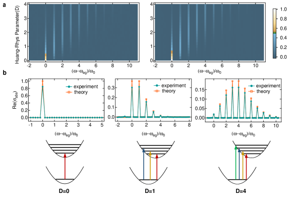
Figure 2: Absorption spectrum of the nuclear system at vacuum ($\ket{\psi}=\ket{0}$) at zero temperature. (a) Progress of the absorption spectrum as a function of Huang-Rhys parameter $D$. Here we only present the real part of $\sigma_{abs}$. The $x$ axis represents the normalized spectral frequency of electronic transition, which describes the necessary energy for transitions from the electronic ground state to the excited states. We compare experimental results (left) with theory (right) using the same color scale which represents the transition probability. (b) The cross section at $D$=0, 1, and 4, and the corresponding schematics of the electronic transitions (bottom row). As expected, the absorption peaks of zero-temperature molecular spectrum arises from $\omega_{eg}$, separated by $\omega_{0}$ with a Poisson distribution of intensities. The experimental data are lower by a constant reduction factor $f=0.83$ than theory, as expected dominantly due to the decoherence of the qubit during the simulation process.

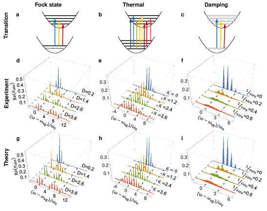
Figure 3: Absorption spectrum of three different initial nuclear states in the molecular system vs different parameters. The top diagrams depict the corresponding electronic transitions: (a) Fock state $\ket{1}$; (b) thermal state; (c) damped vacuum state. The middle and bottom rows show the corresponding experimental results and theoretical expectations, respectively. For clarity, here we only show the typical spectrums with the corresponding parameter next to each plot. For both thermal state and damped vacuum state, $D=1$. Except for a reduction of experimental peak values, the experimental results show good agreement with theoretical expectation.

Figure 4: Progression of spectral peak at $\omega=\omega_{eg}$. Peak values at $\omega=\omega_{eg}$ in Fig. 2 and Fig. 3 as a function of (a) $D$ for an initial vacuum state; (b) $D$ for a Fock state $\ket{1}$; (c) $\bar{n}$ for a thermal equilibrium state; (d) $1/\tau\omega_{0}$ for a damped vacuum state. Dots are experimental data after dividing a constant reduction factor $f$, in good agreement with theoretical expectation depicted in solid curves. $f=0.83$ for a, b, and d while $f=0.75$ for c. The smaller $f$ for the case of Fock state $\ket{1}$ is mainly due to the finite Fock state preparation fidelity $F=0.94$ while all other three cases start from a nearly perfect vacuum state. The standard deviation for each measured value is much less than 0.01 and not shown in the figure.

In this work, we develop and demonstrate a quantum simulation approach for studying molecular dynamics and absorption spectroscopy using a superconducting simulator. Besides simulating molecules in equilibrium, this approach of quantum simulation also allows us to obtain non-equilibrium molecular spectra that are not directly accessible under normal laboratory conditions. In addition, the problem of sampling the absorption spectra of molecules Huh et al. (2015) has been found to be related to the problem of Boson Sampling Aaronson and Arkhipov (2013), which represents a promising approach to justify that quantum simulators cannot be simulated efficiently with any classical means. Our approach is complimentary with the existing approach Huh et al. (2015), where the absorption spectra are obtained by sampling the transition probabilities for each pair of input-output Fock states. The key difference is that we focus on the dynamics of the phonons, instead of the structural shift due to the Duschinsky transformation Peng et al. (2007).

More specifically, our approach can be applied to obtaining the temporal correlation function of the electronic transition dipole Mukamel (1999), which yields the information about the absorption spectrum of the molecule, after applying the Fourier transformation. In our superconducting simulator, there are many adjustable control knobs for simulating the spectra for a variety of scenarios. In particular, we are able to simulate molecules in a wide range of values of the Huang-Rhys parameter $D$, which characterizes the electron-phonon coupling strength.

In this work, we focus on the model approximating the electronic degrees of freedom by a two-level system (Fig. 1a). This model has been applied to study vibronic wavepacket dynamics, chemical reaction rate, Marcus theory for non-adiabatic electron transfer, etc. For molecular spectroscopy, the absorption spectra strongly depend on the initial state of the phonon degree of freedom in the manifold of the electronic ground state. In our experimental demonstration, we have performed simulations by preparing the phonon mode in pure Fock states, as well as simulations for a thermal state and a vacuum state with damping. In all cases, we are able to experimentally observe the progression of absorption peaks separated by the vibronic frequency, which is a characteristic feature of molecular spectrum due to vibronic transitions. This flexibility of our superconducting simulator makes it a useful tool for validating theoretical prediction when scaled up (see Methods section).

The architecture of the superconducting simulator is constructed through a three-dimensional (3D) circuit quantum electrodynamics (QED) system Wallraff et al. (2004); Paik et al. (2011), where a “vertical” transmon qubit is dispersively coupled to two 3D aluminum cavities for storage and readout, as shown in Fig. 1c. The qubit with a transition frequency $\omega_{eg}/2\pi=5.345$ GHz is used to model the electronic state $\{\ket{g},\ket{e}\}$ of the molecule. The storage cavity (hereafter referred as the “cavity” for simplicity) is used to model the quantization of the nuclear vibrational motion, i.e., phonons $\{\ket{0},\ket{1},\ket{2},...\}$, with a frequency $\omega_{0}/2\pi=8.230$ GHz. Note that the energy gap of the qubit is comparable with that of the cavity frequency, i.e., $\omega_{eg}\sim\omega_{0}$. However, for a typical molecule, the phonon frequency is much smaller than that of the electronic excitation gap. Therefore, a direct analog molecular simulation with superconducting qubits is not feasible; such a challenge can be overcome by a digital approach of quantum simulation covered in this work.

The working mechanism of our superconducting simulator is summarized as follows (see Figs. 1b and 1c). First, the qubit is initialized to the ground state $\ket{g}$ while the phonons (cavity) are prepared in certain given state $\left|\psi\right\rangle$ for the purpose of simulating the molecular system initially at different nuclear states. In our experiment, we have prepared different phonon states: (i) a vacuum state at zero temperature, (ii) a Fock state $\ket{1}$ at zero temperature, (iii) a thermal equilibrium state, and (iv) a vacuum state with damping. As an example, the pulse sequence for the case of a Fock state $\ket{1}$ is presented in the Supplementary Materials. The qubit is then through a classical microwave pulse turned into a superposition state $(\ket{g}+\ket{e})/\sqrt{2}$, after applying a $\pi/2$ rotation (a Hadamard transformation).

Next, a controlled-operation ${U_{\text{ctrl}}}$ is applied to the qubit-phonon system, which drives the evolution of the phonons only if the qubit is in $\ket{g}$, i.e., ${U_{\text{ctrl}}}=\left|g\right\rangle\left\langle g\right|\otimes U+\left|e\right\rangle\left\langle e\right|\otimes I$, where the unitary operator, $U(t)\equiv{e^{i{H_{g}}t}}{e^{-i{H_{e}}t}}$, first evolves the phonons for a time interval $t$ with Hamiltonian $H_{e}$, followed by an inverse time evolution with $H_{g}$ for the same time interval. The operation $U$ can be simplified as follows: in the second quantized form, we have the Hamiltonian, ${H_{e}}=\omega_{0}{b^{\dagger}}b+\omega_{eg}$, describing a harmonic oscillator with an equilibrium position shifted by $d$ relative to ${H_{g}}=\omega_{0}{a^{\dagger}}a$, where $b={\cal D}({-\tilde{d}})a{\cal D}({\tilde{d}})=a+{\tilde{d}}$ with $\tilde{d}=d\sqrt{m{\omega_{0}}/2\hbar}$, and ${\cal D}$ a displacement operator. Consequently, the operator $U$ can be implemented as a displacement operator, $U={e^{-i\phi\left(t\right)}}{\cal D}(\tilde{d}({e^{i{\omega_{0}}t}}-1))$, apart from a phase factor ${e^{-i\phi\left(t\right)}}$, where $\phi\left(t\right)\equiv{\omega_{eg}}t+{{\tilde{d}}^{2}}\sin{\omega_{0}}t$ (see Supplementary Materials for derivation details).

Note that this phase factor cannot be ignored, as it yields a relative phase instead of global phase with $U_{\text{ctrl}}$. Experimentally, the phase $\phi$ is realized in the previous $\pi/2$ rotation as an azimuth angle in the $X$-$Y$ plane on the Bloch sphere (Fig. 1c). The controlled displacement operation ${\cal D}^{g}(\bm{\alpha})$, effective only when the qubit is at $\ket{g}$ state as indicated by an extra superscript $g$, is implemented by a broad selective pulse with a Gaussian envelope truncated to $4\sigma=1.34~{}\mu$s (Fig. 1c). Here the displacement vector ${\bm{\alpha}}=\tilde{d}({e^{i{\omega_{0}}t}}-1)$. It is worth noting that the decoherence of the system during this long selective pulse lowers the subsequent qubit measurement contrast by a factor of about 0.83 compared to the ideal case.

Finally, as a result the dipole correlation function defined as ${C_{\mu\mu}}(t)={\left\langle\psi\right|U(t)\left|\psi\right\rangle}$ is encoded in the off-diagonal elements of the reduced density matrix of the qubit, i.e., ${C_{\mu\mu}}\left(t\right)=\left\langle{{\sigma_{x}}}\right\rangle+i\left\langle{{\sigma_{y}}}\right\rangle$. $\left\langle{{\sigma_{y}}}\right\rangle$ and $\left\langle{{\sigma_{x}}}\right\rangle$ of the qubit can be measured by applying an extra $\pi/2$ rotations along $X$ and $Y$ axis ($R_{XorY}$) respectively followed by a $Z$-basis measurement. This general procedure is applicable for any initial state of the phonon, pure or mixed. The absorption spectrum ${\sigma_{{\text{abs}}}}$ is finally obtained by a Fourier transform of ${C_{\mu\mu}}(t)$.

We follow the above procedure to simulate the molecular system initially at a vacuum state and a Fock state $\ket{1}$ at zero temperature. However, in order to simulate molecular spectra with the phonon mode initialized in a thermal state, $\rho\equiv{e^{-{\hbar\omega_{0}}{a^{\dagger}}a/kT}}/{\text{Tr}}({e^{-{\hbar\omega_{0}}{a^{\dagger}}a/kT}})$, it is not practical to increase the physical temperature, as the performance of the experimental system would decrease significantly. To overcome this challenge, we can modify the above procedure at Step 1: instead of an equal superposition (after a Hadamard gate), the qubit is initialized to ${e^{-i\phi(t)}}\sin{\frac{\gamma(t)}{2}}\ket{g}+\cos{\frac{\gamma(t)}{2}}\ket{e}$, where the angle $\gamma(t)$ is chosen such that $\sin\gamma=e^{2\tilde{d}^{2}\bar{n}(\cos\omega_{0}t-1)}$ and $\bar{n}=(e^{\hbar\omega_{0}/kT}-1)^{-1}$ (see Supplementary Materials). Similarly, for the case of a vacuum state with damping, we choose $\sin\gamma(t)={e^{-t/\tau}}$, where $\tau$ is the characteristic time (also see Supplementary Materials). In both cases, following the same remaining procedure as described above, one can obtain the correlation function ${C_{\mu\mu}^{thm}}\left(t\right)$ for an initial thermal state and the damped correlation function $C_{\mu\mu}^{{\text{damp}}}\left(t\right)={e^{-t/\tau}}{C_{\mu\mu}}\left(t\right)$, respectively.

Our experimental results are as follows. In our digital simulation, we have set $\Delta t=1$, $t_{max}=900$, $\omega_{eg}=\pi/5$, $\omega_{0}=\pi/90$. The spectrum lineshape of molecule illustrates the relative probability of electronic transition between different vibrational states in nuclear space. In Fig. 2, we present the progression of absorption peaks for the case where the phonon state is initialized at vacuum and at zero temperature, $\left|\psi\right\rangle=\left|0\right\rangle$, for various Huang-Rhys parameter $D={\tilde{d}}^{2}$. When $D=0$, there is only a sharp peak located at the frequency $\omega=\omega_{eg}$. This case represents the limit where the electronic transition and the nuclear motion are decoupled. In other words, the molecule is essentially the same as a two-level atom, as far as the spectrum is concerned. When $D$ is increased from zero to, e.g., $D=1$, several peaks emerge, and these peaks are equally spaced by the phonon frequency $\omega_{0}$. When $D$ is increased further to $D=4$, we can observe more equally-spaced peaks. However, the amplitude of the direct transition at $\omega=\omega_{eg}$ is no longer the largest. In all experimental trials, except for a reduction factor $f=0.83$ mainly due to the qubit decoherence, the spectral peaks are in good agreement with the expected Poisson distribution (see Methods).

The absorption spectrum of the other three different initial nuclear states in the molecular system are shown in Fig. 3: (i) Fock state $\ket{1}$ with different $D$; (ii) thermal equilibrium state at different temperatures characterized by the occupation number $\bar{n}$; and (iii) damped vacuum state with different dissipation rates described by the characteristic time $\tau$. The corresponding electronic transitions for each case have been depicted in the top diagrams of Fig. 3. For clarity, we only show the typical spectra. Except for a reduction of experimental peak values, the experimental results show good agreement with theoretical expectation.

One of the key features of our quantum simulator is that the parameters, such as Huang-Rhys parameter $D$, can be varied continuously. To better illustrate the progression of the spectrum in Fig. 2 and Fig. 3 as a function of various parameters, we present the peak values at $\omega=\omega_{eg}$ as an example in Fig. 4. Dots are experimental data by our quantum simulator while the solid curves represent theoretical expectation. After taking into account the reduction of experimental peak values, again mainly due to the system decoherence, by dividing a constant reduction factor $f$ ($f=0.83$ for Figs. 4a, 4c, and 4d; $f=0.75$ for Fig. 4b), the experimental results are in good agreement with theoretical expectations. The smaller $f$ for the case of Fock state $\ket{1}$ is mainly due to the finite Fock state preparation fidelity $F=0.94$ (measured Wigner function shown in Supplementary Materials) while all other three cases start from a nearly perfect vacuum state.

To conclude, we demonstrated experimentally a new method to simulate electronic absorption spectra of a molecule, where the nuclear vibrational states may or may not be in thermal equilibrium. Our quantum simulator is based on a superconducting circuit QED architecture with flexible parameter tunability. The simulation results indicate that the resulting molecular spectra are in good agreement with theoretical expectation. Finally, we note that this method can be readily extended to other quantum simulation platform, including photonic Aspuru-Guzik and Walther (2012) or trapped-ion Kim et al. (2010) systems. Therefore, our experiment represents the beginning of a new approach of predicting molecular spectroscopy using quantum simulators.

.1 Device parameters.

The transmon qubit has an energy-relaxation time $T_{1}=13~{}\mu$s and a pure dephasing time $T_{\phi}=16~{}\mu$s. The storage cavity has a lifetime $\tau_{0}=80~{}\mu$s. The readout cavity has a transition frequency $\omega_{m}/2\pi=7.291$ GHz and a lifetime $\tau_{r}=42$ ns. Together with a Josephson parametric amplifier Hatridge et al. (2011); Roy et al. (2015) operating in a double-pumped mode Kamal et al. (2009); Murch et al. (2013), the fast readout cavity is used for a high fidelity and quantum non-demolition detection of the qubit state (see Supplementary Materials for details). Experimental setup details can also be found in Ref. Liu et al. (2016). The qubit-state-dependent frequency shift of the storage cavity is $\chi_{qs}/2\pi=-1.44$ MHz, allowing for the qubit-controlled operation on the cavity state as used in our experiment.

.2 Molecular Hamiltonian.

Under the standard Born-Oppenheimer framework, the Hamiltonian $H_{\rm mol}$ of a molecule depends on the nuclear configuration (i.e., position coordinates) $\bm{q}$ as parameters, ${{H_{\text{mol}}(\bm{r},\bm{q})}}={K_{\text{e}}}+{U_{{\text{ee}}}}\left({\bm{r}}\right)+{U_{\text{eN}}}\left({{{\bm{r}},{\bm{q}}}}\right)$, where ${K_{\text{e}}}$ is the kinetic-energy term for the electrons, ${U_{{\text{ee}}}}\left({\bm{r}}\right)$ and ${U_{\text{eN}}}\left({{{\bm{r}},{\bm{q}}}}\right)$ are the electron-electron interaction term and electron-nuclei interaction term respectively. In the low-energy sector, the molecule typically contains an electronic ground state $\ket{g}$ and an excited state $\ket{e}$, where the molecular Hamiltonian becomes:

$$H_{\rm mol}({\bm{q}})=H_{g}(\bm{q})\ket{g}\bra{g}+H_{e}(\bm{q})\ket{e}\bra{e}\ ,$$ (1)

with $H_{g}=K_{\rm N}+V_{g}(\bm{q})$ and $H_{e}=K_{\rm N}+V_{e}(\bm{q})$. Here $K_{\rm N}$ is the nuclear kinetic energy, $V_{g}(\bm{q})$ and $V_{e}(\bm{q})$ are the potential energies, which are typically approximated as harmonic functions (Fig. 1a), i.e., ${H_{g}}=\tfrac{1}{{2m}}{p^{2}}+\tfrac{{m{\omega_{0}^{2}}}}{2}{q^{2}}$ and ${H_{e}}=\tfrac{1}{{2m}}{p^{2}}+\tfrac{{m{\omega_{0}^{2}}}}{2}{(q-d)^{2}}+{\hbar\omega_{eg}}$. Here $\omega_{eg}$ is the electronic gap between the minima of both potentials (i.e., 0-0 energy splitting).

.3 Franck-Condon approximation.

The coupling strength between the electronic transition and the nuclear motion is characterized by the Huang-Rhys parameter, $D=\tilde{d}^{2}$, where $\tilde{d}=d\sqrt{m{\omega_{0}}/2\hbar}$. Similarly, the electronic transition dipole operator is given by $\mu(\bm{q})=\mu_{eg}(\bm{q})\ket{e}\bra{g}+\mu_{ge}(\bm{q})\ket{g}\bra{e}$. However, the dependence of electronic transition moment on nuclear is usually insensitive to the nuclear motion; one can therefore approximate (known as Condon approximation) it with a constant, i.e., $\mu_{eg}(\bm{q})=\mu_{ge}(\bm{q})=1$ for simplicity.

.4 Absorption lineshape.

The absorption line shape, $\sigma_{{\text{abs}}}\left(\omega\right)=\int_{-\infty}^{\infty}{dt}\ {e^{i\omega t}}\ {C_{\mu\mu}}\left(t\right)$, can be obtained by the Fourier transform of the dipole correlation function ${C_{\mu\mu}}\left(t\right)\equiv\left\langle{\mu\left(t\right)\mu\left(0\right)}\right\rangle$, where $\mu\left(t\right)={e^{i{H_{{\text{mol}}}}t/\hbar}}{\mu(0)}\ {e^{-i{H_{{\text{mol}}}}t/\hbar}}$. In order to mimic the effects on the molecular spectra due to the influence of the environment Kroto (1992), one can append a damping factor ${e^{-t/\tau}}$ to the above correlation function, i.e., $C_{\mu\mu}^{{\text{damp}}}\left(t\right)={e^{-t/\tau}}{C_{\mu\mu}}\left(t\right)$, which yields a spectrum with line broadening $\sigma_{{\text{abs}}}^{{\text{damp}}}\left(\omega\right)$. Our main task is to apply our superconducting simulator to obtain the correlation functions for the molecules to be simulated. For example, if the initial state is a vacuum state, the correlation function $C_{\mu\mu}\left(t\right)=e^{-i\omega_{eg}t}e^{D(e^{-i\omega_{0}t}-1)}$. The absorption lineshape is $\sigma_{{\text{abs}}}\left(\omega\right)=e^{-D}\int_{-\infty}^{\infty}{dt}\ e^{i\omega t}\ e^{-i\omega_{eg}t}e^{De^{-i\omega_{0}t}}$. By expanding $e^{De^{-i\omega_{0}t}}=\sum_{j=0}^{\infty}\frac{1}{j!}\left(De^{-i\omega_{0}t}\right)^{j}$, the lineshape becomes $\sigma_{{\text{abs}}}\left(\omega\right)=e^{-D}\sum_{j=0}^{\infty}\frac{D^{j}}{j!}\delta\left(\omega-\omega_{eg}-j\omega_{0}\right)$. Thus the spectral peaks are separated by $\omega_{0}$ with a Poisson distribution of intensities.

.5 Scalability.

Our approach can be scaled up for molecules with multiple vibronic modes. In this case, the dipole correlation function comes from the contributions of the individual modes, i.e., for $n$ modes, ${C_{\mu\mu}}\left(t\right)={\left|{{\mu_{eg}}}\right|^{2}}{e^{-i\left({{E_{e}}-{E_{g}}}\right)t/\hbar}}{F_{n}}\left(t\right)$, where ${F_{n}}\left(t\right)={\rm Tr}\left({{e^{i{H_{g}}t/\hbar}}{e^{-i{H_{e}}t/\hbar}}{\rho_{1}}\otimes{\rho_{2}}\cdots\otimes{\rho_{n}}}\right)$. In other words, the superconducting qubit needs to be coupled with multiple cavity modes. This direction has been realized experimentally Wang et al. (2016). There, a superconducting qubit is coupled to two cavity modes to realize an entangled pair of single-cavity cat states. With a similar geometry, the superconducting qubit can easily be extended to couple to more cavity modes.