Levitation of heavy particles against gravity in asymptotically downward flows

Abstract

In the fluid transport of particles, it is generally expected that heavy particles carried by a laminar fluid flow moving downward will also move downward. We establish a theory to show, however, that particles can be dynamically levitated and lifted by interacting vortices in such flows, thereby moving against gravity and the asymptotic direction of the flow, even when they are orders of magnitude denser than the fluid. The particle levitation is rigorously demonstrated for potential flows and supported by simulations for viscous flows. We suggest that this counterintuitive effect has potential implications for the air-transport of water droplets and the lifting of sediments in water.

Levitation—the action of rising and hovering in apparent defiance of gravity—is a fascinating phenomenon with many practical implications. A classic demonstration is the Bernoulli ball levitation, in which a macroscopic particle heavier than air (such as a ping pong ball) can levitate in response to an inclined upward air stream that appears to only partially balance gravity. A key aspect of that form of levitation is the transversal stability due to the Coandǎ effect,[1] which relies on the tendency of the flow to curve around the surface of the ball and sustains stable levitation when the upward air stream is tilted. Here, we report a new form of fluid-dynamical levitation that can be observed even for a downward stream (i.e., in the direction of gravity) and that allows heavy particles to be levitated by a flow regardless of whether they are 10, 100, or 1,000 times denser than the fluid. This phenomenon is fundamentally different from the Coandǎ effect in that it concerns microscopic heavy particles and requires no disturbance of the flow by the particles.

Many natural and industrial flows transport small particles, like droplets, sediments, and microorganisms. [2] Inertial effects cause the trajectories of such particles to deviate from the streamlines of the flow, making the study of particle-laden flows challenging both theoretically and experimentally. [3, 4, 5, 6] Key to such studies are the dissipative nature of the advection dynamics and the consequent tendency of the particles to accumulate in specific zones of the flow domain, both in closed flows [7, 8, 9, 10, 11, 12, 13, 16, 14, 17, 14, 15] and in open flows, [22, 21, 19, 20, 18] even when the flows are incompressible. For example, particles less dense than the fluid tend to be attracted to the interior of vortices, [23, 24] which can lead to the formation of attractors for the particle dynamics independently of the global properties of flow. Particles denser than the fluid, on the other hand, tend to be repelled by vortices, which is a mechanism that can lead to the formation of attractors if the flow is closed; this effect, which is also related to the preferential trajectories phenomenon, [9] has been widely investigated over the past two decades. [3] However, much less is known about dense particles moving in flows that have unbounded streamlines and are therefore open. In open flows, an outstanding problem of particular interest concerns the transport of small particles much denser than the fluid, which we term heavy particles and which can represent for example water droplets in the air.

In this article, we demonstrate the possibility of levitation and upward transport of heavy particles by a flow moving asymptotically downward, even in the presence of gravity. Because at first these conditions seem to facilitate downward advection, one might expect that all particles would necessarily fall, which is in sharp contrast with the effect we report. The starting point of our analysis is the observation that such a flow can support pairs of mutually interacting vortices traveling in a direction that opposes the flow. We thus focus on asymptotically simple flows that move downward and have a pair of vortices moving upward. Using this class of flows we show that attracting points (dimension-zero attractors) formed near the center of vorticity can capture heavy particles released at any distance above the vortices. For this to occur, particle inertia must allow for particles to approach the vortices and for the existence of attractors to retain them in that region; we show that these two conditions are satisfied for a wide range of Stokes number in the class of flows we consider. This is demonstrated analytically using asymptotic analysis and Melnikov functions, and is illustrated numerically using simulations in both inviscid and viscous laminar flows.

Our analysis is inspired by previous experimental realizations of flows with pairs of interacting vortices [25, 26, 27, 28, 29] and theoretical work on particle advection in such flows. [19, 16, 17, 18, 15, 33, 32, 31, 30] Several studies have shown, both numerically [19] and analytically, [16, 17, 18] the formation of attractors for the dynamics of heavy particles in the vicinity of identical co-rotating vortices. Different work has shown that such attractors persist for non-identical vortices in closed potential flows in the absence of gravity, [15] but no results exist for open flows, viscous regimes, or the effects of gravity. Here, in order to demonstrate the proposed levitation of heavy particles, we first generalize the special results in open flows, previously established for nongeneric vortex pairs, to the case of (i) generic pairs of both co-rotating and counter-rotating vortices of arbitrary vortex strength ratio, (ii) for vortices moving against a background flow that is co-directional with gravity, and (iii) for both potential and viscous flows. Under these general conditions we then show the existence of attracting points that capture heavy particles from both the closed and open flow regions and carry them against gravity and the background flow.

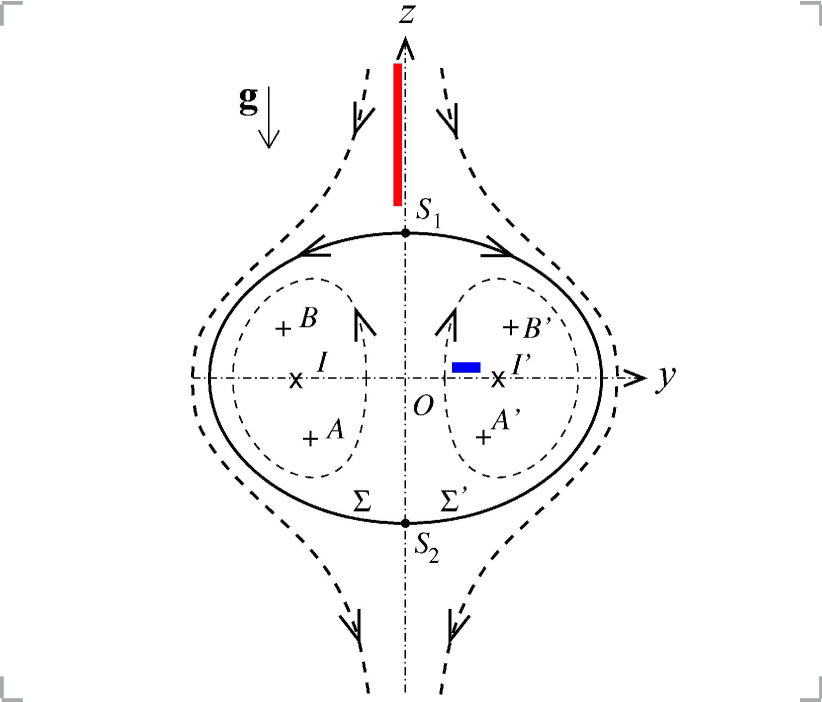
Figure 1: Sketch of the flow: vortices $A$ and $B$ and their mirrors together with typical streamlines (dashed lines) in the reference frame of the centers of vorticity $I$ and $I^{\prime}$. The flow along the open streamlines moves downward—the orientation of the gravitational field, $\mathbf{g}$. Also shown is where the particles are initiated (with the velocity of the flow) in the potential flow simulations below: blue and red particles are released in the closed and open regions of the flow, respectively.

The model flow is depicted in Fig. 1. It consists of two vortices, $A$ and $B$, with strengths $\Gamma_{A}$ and $\Gamma_{B}$, respectively, plus mirror vortices $A^{\prime}$ and $B^{\prime}$ with opposite strengths and symmetric positions with respect to the vertical axis $Oz$. This axis can be regarded as a “wall” in the framework of potential flow theory used in our calculations. The position $\mathbf{r}_{I}$ of the center of vorticity $I$ of the pair $(A,B)$ is $\mathbf{r}_{I}=({\Gamma_{A}\mathbf{r}_{A}+\Gamma_{B}\mathbf{r}_{B}})/({\Gamma_{A}+\Gamma_{B}}),$ where $\mathbf{r}_{A}$ is the position of $A$ and $\mathbf{r}_{B}$ is the position of $B$. In the absence of mirror vortices, point $I$ remains fixed and $AB$ rotates steadily around $I$ with angular velocity $\Omega_{0}=({\Gamma_{A}+\Gamma_{B}})/({8\pi d_{0}^{2}}),$ where $2d_{0}=|AB|$ is the distance between the vortices, which remains constant in this case. When the two pairs $(A,B)$ and $(A^{\prime},B^{\prime})$ are close enough to interact, elementary vortex dynamics show that point $I$ moves vertically, and its distance to the symmetry axis $Oz$ remains equal to its initial value, $L_{0}$. For $d_{0}\ll L_{0}$, the (vertical) velocity of $I$ approaches $w_{0}=({\Gamma_{A}+\Gamma_{B}})/{4\pi L_{0}}$ in the frame of the fluid at infinity. The streamfunction of the exact 2D potential flow induced by the four vortices, in the frame translating at constant speed $w_{0}\,\hat{\mathbf{z}}$, where $\hat{\mathbf{z}}$ is the upward unit vector, is

$$\psi(\mathbf{r},t)=\frac{\Gamma_{A}}{4\pi}\ln\frac{|\mathbf{r}-\mathbf{\bar{r}}_{A}|^{2}}{|\mathbf{r}-\mathbf{r}_{A}|^{2}}+\frac{\Gamma_{B}}{4\pi}\ln\frac{|\mathbf{r}-\mathbf{\bar{r}}_{B}|^{2}}{|\mathbf{r}-\mathbf{r}_{B}|^{2}}+w_{0}\,y,$$ (1)

where $\mathbf{r}=(y,z)$, and $\mathbf{\bar{r}}_{A}$ and $\mathbf{\bar{r}}_{B}$ are the positions of the mirror vortices $A^{\prime}$ and $B^{\prime}$, respectively. The instantaneous velocity of fluid elements in this frame trace closed streamlines near the vortices (closed flow region) and open streamlines further away from them (open flow region). As indicated in Fig. 1, these two regions meet along the separatrix streamline $\Sigma$ joining the stagnation points located on the $z$-axis, $S_{1}$ and $S_{2}$. The structure formed by $\Sigma\cup S_{2}S_{1}$ is a heteroclinic cycle for the dynamics of fluid elements; heteroclinic (and homoclinic) cycles are generally expected to play a role in the transport of both non-inertial and inertial particles. [34, 3]

To proceed, we define $\gamma=\Gamma_{A}/\Gamma_{B}$ as the vortex strength ratio, where $-1<\gamma\leq 1$. It can be checked that up to order $\varepsilon^{2}$, when $\varepsilon\equiv d_{0}/L_{0}<(\gamma+1)/2$, $A$ and $B$ rotate around $I$ approximately as a rigid body with angular velocity $\Omega_{0}$. This allows us to write $\mathbf{r}_{A,B}(t)$ and ${\mathbf{\bar{r}}_{A,B}}(t)$ in the form of $2\pi/\Omega_{0}$-periodic functions plus $O(\varepsilon^{2})$ corrections. Throughout the rest of the article we operate with the equations in non-dimensional form, using as units $L_{0}$ for lengths and $w_{0}/2$ for velocities since these choices capture the appropriate orders of magnitude for the flow near the heteroclinic cycle $\Sigma$. (No new notation is introduced for non-dimensional variables.) Expanding Eq. (1) in powers of $\varepsilon$, in non-dimensional form the streamfunction reads

$$\psi(\mathbf{r},t)\!=\!\psi_{0}(\mathbf{r})+\frac{4\gamma\varepsilon^{2}}{(1\!+\!\gamma)^{2}}\,\!\!\Big{[}\psi_{2c}(\mathbf{r})\cos\frac{2t}{\varepsilon^{2}}+\psi_{2s}(\mathbf{r})\sin\frac{2t}{\varepsilon^{2}}\Big{]}\!\!\!$$ (2)

plus $O(\varepsilon^{3})$ terms, where the components $\psi_{0},\,\psi_{2c},\,\psi_{2s}$ are identical to those for the case $\gamma=1$ [35] given that the $\gamma$-dependence is accounted for by the prefactor (see supplementary material). The remainder in Eq. (2) can be shown to be $O(\varepsilon^{4})$ when $\gamma=1$. The velocity field—defined as $\mathbf{u}=\mathbf{\nabla}\times(\psi\,\hat{\mathbf{x}})$, where $\hat{\mathbf{x}}$ is the right handed unit vector orthogonal to the $yz$ plane—is therefore of the form $\mathbf{u}(\mathbf{r},t)=\mathbf{u}_{0}(\mathbf{r})+\varepsilon^{2}\mathbf{u}_{2}(\mathbf{r},t/\varepsilon^{2};\gamma)+O(\varepsilon^{3})$, where $\mathbf{u}_{2}$ is time-periodic with period $T=\pi\varepsilon^{2}$ and corresponds to the leading perturbation induced by the rotation of the vortices.

Having established the fluid flow equations, we now write the particle equation of motion in this flow. For a heavy particle with small particle Reynolds number, the non-dimensional equation is $\ddot{\mathbf{r}}={\widetilde{\rm St}}^{-1}\left[{\mathbf{u}}(\mathbf{r},t)+\widetilde{\mathbf{V}}_{T}-\dot{\mathbf{r}}\right]$, where $\mathbf{r}$ is the particle position, $\widetilde{\mathbf{V}}_{T}=-\widetilde{V}_{T}\hat{\mathbf{z}}=-2(g\,\tau_{p}/w_{0})\hat{\mathbf{z}}$ is the free-fall terminal velocity, and $\widetilde{\rm St}$ is the Stokes number (i.e., the response time of the particle, $\tau_{p}$, divided by the time-scale of the flow, $2L_{0}/w_{0}$). [36] We also introduce another Stokes number, ${\rm St}=\Omega_{0}\,\tau_{p}$, to describe the dynamics of particles directly influenced by the rotation of the vortices around each other. The formation of attractors near the vortices requires that ${\rm St}$ be no larger than order one since drag has to balance centrifugal force in this case. We therefore assume ${\rm St}=O(1)$, so that $\widetilde{\rm St}\equiv\varepsilon^{2}{\rm St}\ll 1$ and the equation for $\mathbf{r}$ can be reduced to

$$\dot{\mathbf{r}}={\mathbf{v}}_{0}(\mathbf{r})+\varepsilon^{2}{\mathbf{v}}_{2}(\mathbf{r},t/\varepsilon^{2};\gamma)+O(\varepsilon^{3}),$$ (3)

where $\mathbf{v}_{0}(\mathbf{r})={\mathbf{u}}_{0}(\mathbf{r})+\widetilde{\mathbf{V}}_{T}$ and $\mathbf{v}_{2}(\mathbf{r},\tau;\gamma)\simeq\mathbf{u}_{2}({\mathbf{r}},\tau;\gamma)-{\rm St}\big{[}({\mathbf{u}}_{0}+\widetilde{\mathbf{V}}_{T}).\nabla{\mathbf{u}}_{0}+{\partial{\mathbf{u}}_{2}(\mathbf{r},\tau;\gamma)}/{\partial\tau}\big{]},$ for $\tau=t/\varepsilon^{2}$ (see also Ref. [37]). We show that the particle dynamics described by this equation have at least one (for $-1<\gamma\leq 1$) and possibly two attracting points (for $0<\gamma\leq 1$), provided that the Stokes number is not too large (see supplementary material).

In Eq. (3), the leading term, ${\mathbf{v}}_{0}$, represents the conservative dynamics of non-inertial particles in a steady flow induced by the equivalent to a single vortex with strength $\Gamma_{A}+\Gamma_{B}$ (together with its mirror) plus a uniform flow $-\widetilde{V}_{T}\hat{\mathbf{z}}$. The particle streamfunction for this term, $\psi_{p}(y,z)=\psi_{0}(y,z)+y\widetilde{V}_{T}$, is time-independent (a similar streamfunction has been used to describe plankton dynamics [38]). The first perturbative term, $\varepsilon^{2}{\mathbf{v}}_{2}$, contains the contribution $\mathbf{u}_{2}$ of the unsteadiness of the flow due to the fact that for $\varepsilon>0$ there are two vortices rather than one, and also the effect of inertia in the ${\rm St}$ terms. It is thus convenient to regard this system as a time-independent Hamiltonian $\psi_{p}$ perturbed by dissipative and fast periodic terms. [39] To leading order in $\varepsilon$, the trajectories of the particles coincide with the curves $\psi_{p}(y,z)=$ cte. These curves correspond to open streamlines separated from closed streamlines by a heteroclinic cycle, which we denote $\Sigma_{p}$ and which is the particle analog of $\Sigma$ in Fig. 1 except that $\Sigma_{p}$ does not include the time-dependent perturbation terms.

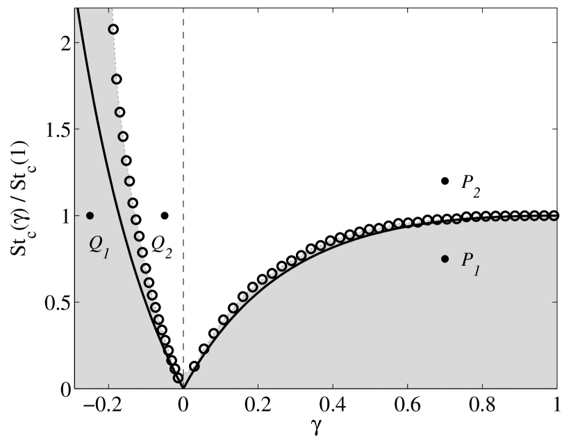
Figure 2: Normalized critical Stokes number for arbitrary vortex strength ratio, $\gamma$. Circles represent simulations for $\widetilde{V}_{T}=0.1$ and $\varepsilon=0.35$, whereas solid lines represent the theoretical prediction in Eq. (7). Particles released in the open flow with ${\rm St}$ in the shaded area may cross $\Sigma_{p}$ and hence be levitated, while those above it cannot.

An important necessary condition for particles from the open flow to be captured by attracting points in the vicinity of the vortices is that they cross $\Sigma_{p}$ (the separatrix of the unperturbed dynamics) under the effect of the motion of the vortices. The occurrence of separatrix crossing can be predicted employing a construction based on separatrix maps. [40, 41] We consider a solution $\mathbf{r}(t)$ of the perturbed system (up to order $\varepsilon^{2}$) and define $t_{n}\,(n=1,2,...)$ as the times at which the particle crosses the axis $Oy$ downward. We also use $\tau_{2n}$ and $\tau_{2n+1}$ to denote the times the particle passes closest to the saddle points $S_{1}$ and $S_{2}$, respectively, and $H_{n}=\psi_{p}[\mathbf{r}(\tau_{2n})]$ and $H_{n+1}=\psi_{p}[\mathbf{r}(\tau_{2n+1})]$ to denote the corresponding values of the unperturbed Hamiltonian. Oscillations of $H_{n+1}-H_{n}$ around zero as $n$ varies will indicate that the separatrix $\Sigma_{p}$ is crossed. Assuming that $\mathbf{r}(t)\simeq\mathbf{q}(t-t_{n})$, for $\mathbf{q}(t)$ denoting the solution of the unperturbed system along $\Sigma_{p}$, we obtain

$$\vspace{-2mm}H_{n+1}-H_{n}\simeq\varepsilon^{2}M(t_{n}),$$ (4)

where $M(t_{n})$ is the Melnikov function associated with $\Sigma_{p}$:

$$\vspace{-2mm}M(t_{n})=\frac{4\gamma(a+\widetilde{V}_{T}b)}{(1+\gamma)^{2}}\Big{[}\sin\frac{2t_{n}}{\varepsilon^{2}}-2{\rm St}\cos\frac{2t_{n}}{\varepsilon^{2}}\Big{]}-m\,{\rm St}$$ (5)

(see supplementary material for details). Here, the amplitudes $a=a(\varepsilon)$ and $b=b(\varepsilon)$ are functions of $\varepsilon$ only, and $m$ is a constant accounting for the centrifugal effect along $\Sigma_{p}$ due to the particle’s inertia.

The Melnikov function in Eq. (5) is either strictly negative or oscillates between positive and negative values. [42] When the function has a constant negative sign, we have $H_{n+1}<H_{n}$ for all $n$, which indicates that particles are centrifuged away from the vortices. When the function has simple zeros, particles can enter and exit the closed flow. Thus, the central prediction of our theory is that a heavy particle in the open flow may be captured by an attracting point near the vortices provided that the Stokes number ${\rm St}$ is below the critical value

$${\rm St}_{c}(\gamma)=\frac{4\mid\gamma\mid}{m(1+\gamma)^{2}}\Big{[}a(\varepsilon)+\widetilde{V}_{T}b(\varepsilon)\Big{]},$$ (6)

which is the condition for $M(t_{n})$ to change sign (and in fact have infinitely many isolated zeros). We therefore predict that the levitation of heavy particles released in the open flow region above the vortices is possible for ${\rm St}<{\rm St}_{c}(\gamma)$. These results imply that heavy particles with densities across many orders of magnitude can be levitated by the same flow. [43]

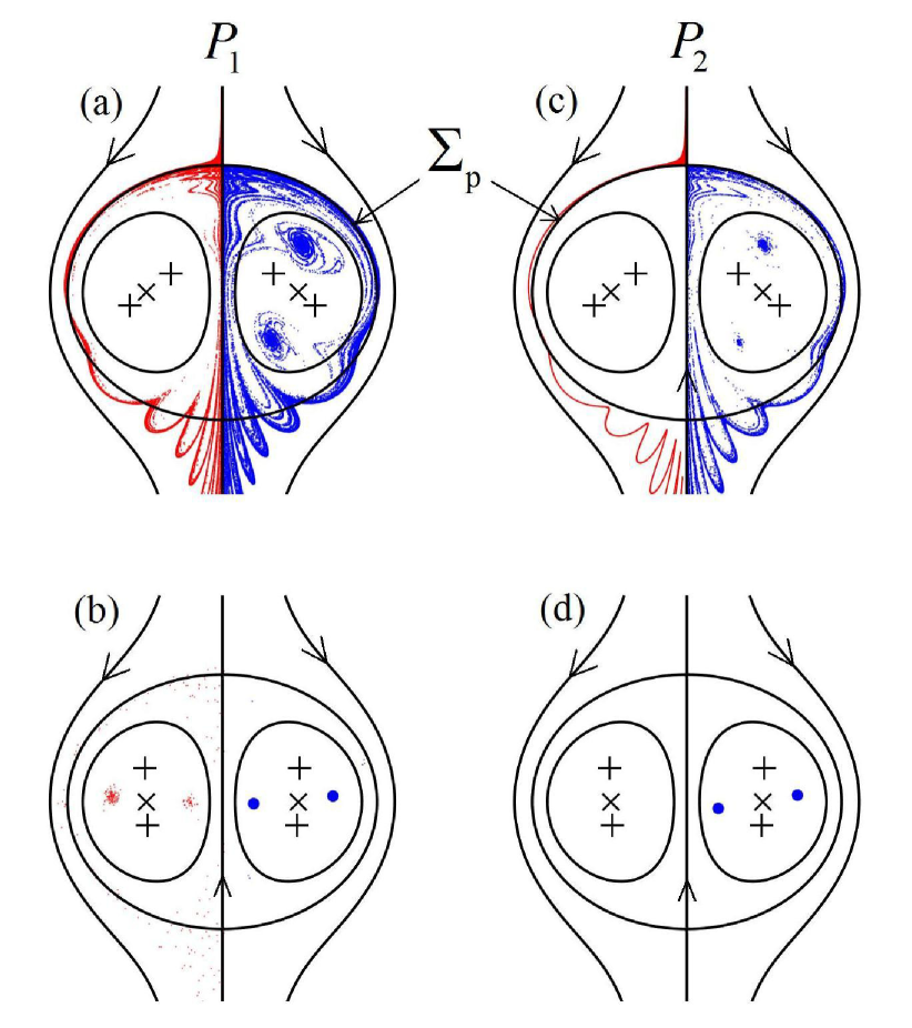
Figure 3: Levitation by co-rotating vortices for the flow in Eq. 1. Colors indicate particle clouds at different times for (a, b) point $P_{1}$ (${\rm St}<{\rm St}_{c}$) and (c, d) point $P_{2}$ (${\rm St}>{\rm St}_{c}$) in Fig. 2. The first row [(a) and (c)] corresponds to $t=16$ and second row [(b) and (d)] to $t=95$ (in units of the undisturbed turnover time, $2\pi/\Omega_{0}$). Also shown are streamlines defined by $\psi_{p}(y,z)=cte$ (continuous lines), the vortices ($+$), and the center of vorticity ($\times$). Red and blue represent particles released from the open and closed flows, respectively, and are shown on opposite sides of the wall to facilitate visualization.

Remarkably, Eq. (6) shows that ${\rm St}_{c}$ is an increasing function of $\widetilde{V}_{T}$ and hence that gravity facilitates levitation. This means that a particle that would be too inertial to penetrate inside $\Sigma_{p}$ in the absence of gravity can be captured by the attracting points when gravity is present. This equation also shows that ${\rm St}_{c}$ depends on the vortex strength ratio $\gamma$ and in particular that the normalized critical Stokes number is

$$\frac{{\rm St}_{c}(\gamma)}{{\rm St}_{c}(1)}=\frac{4\mid\gamma\mid}{(1+\gamma)^{2}},$$ (7)

irrespective of $\widetilde{V}_{T}$ and $\varepsilon$. Thus, not only levitation is possible for both co- and counter-rotating vortices of arbitrary $\gamma\neq-1$, but also the phenomenon is more pronounced for counter-rotating vortices with sufficiently small $\gamma$ than for identical co-rotating vortices ($\gamma=1$).

Figure 2 shows the analytical prediction in Eq. (7) along with a numerical verification for particles released in the open flow above the vortices (red region in Fig. 1), where bisection in ${\rm St}$ was used to determine the critical value at which particles start crossing $\Sigma_{p}$. The agreement with the numerics is good, particularly for co-rotating vortices. Importantly, the numerical ${\rm St}_{c}$ is always higher than the theoretical prediction, widening the range of the effect. [44]

To further illustrate the theoretical results above we have done a series of computations by choosing the parameters according to the diagram of Fig. 2. Figure 3 shows the evolution of clouds of particles for two different Stokes numbers in the case of co-rotating vortices: ${\rm St}<{\rm St}_{c}$ [Fig. 3(a, b)] and ${\rm St}>{\rm St}_{c}$ [Fig. 3(c, d)], corresponding to the points $P_{1}$ and $P_{2}$ in Fig. 2, respectively. The particles are released in the open-streamline region above the vortices (red) and in the closed-streamline region near the vortices (blue), as sketched in Fig. 1. The clouds are shown after $16$ turnover times [Fig. 3(a, c)] and after $95$ turnover times [Fig. 3(b, d)], which was chosen purposely large to facilitate visualization of the long-term behavior. For $P_{1}$, a fraction of the blue particles as well as a fraction of the red particles accumulate near the two attracting points after long times. (For visualization, particles near the attracting points were slightly dispersed). In contrast, for $P_{2}$ only blue particles are captured by the attracting points; red particles remain outside $\Sigma_{p}$ and are transported downstream. These observations are in complete agreement with our predictions.

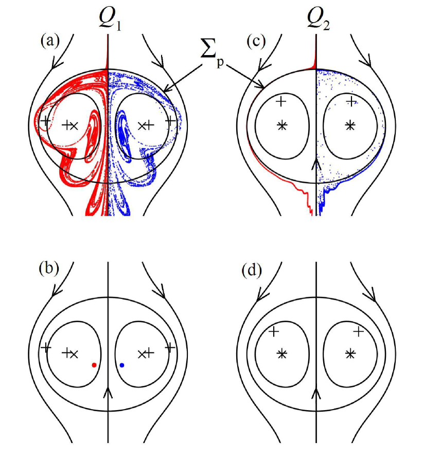
Figure 4: Levitation by counter-rotating vortices. Counterpart of Fig. 3 for (a, b) point $Q_{1}$ (${\rm St}<{\rm St}_{c}$) and (c, d) point $Q_{2}$ (${\rm St}>{\rm St}_{c}$) in Fig. 2. The first row [(a) and (c)] corresponds to $t=21$ and the second row [(b) and (d)] to $t=127$. As in the case of co–rotating vortices, $\Sigma_{p}$ is open to particles released outside when ${\rm St}<{\rm St}_{c}$ and closed to those particles when ${\rm St}>{\rm St}_{c}$. Here there is, however, a single attracting point for each vortex pair for $Q_{1}$ and none for $Q_{2}$.

Similar agreement is observed for counter-rotating vortices, as shown in Fig. 4 for ${\rm St}<{\rm St}_{c}$ ($Q_{1}$ in Fig. 2) and ${\rm St}>{\rm St}_{c}$ ($Q_{2}$ in Fig. 2), but with two important differences. First, in the case of $Q_{1}$ there is only one attracting point around which a portion of blue and red particles accumulate. This is expected for the range of Stokes number considered, but studies of isolated counter-rotating pairs suggest that other attractors may exist for different parameters. [15] Second, for $Q_{2}$, there is no attractor, so that not only do red particles not cross $\Sigma_{p}$ inward, but also all blue particles are centrifuged outward across $\Sigma_{p}$. As a result, in this case no particle is captured by an attractor independently of the initial condition.

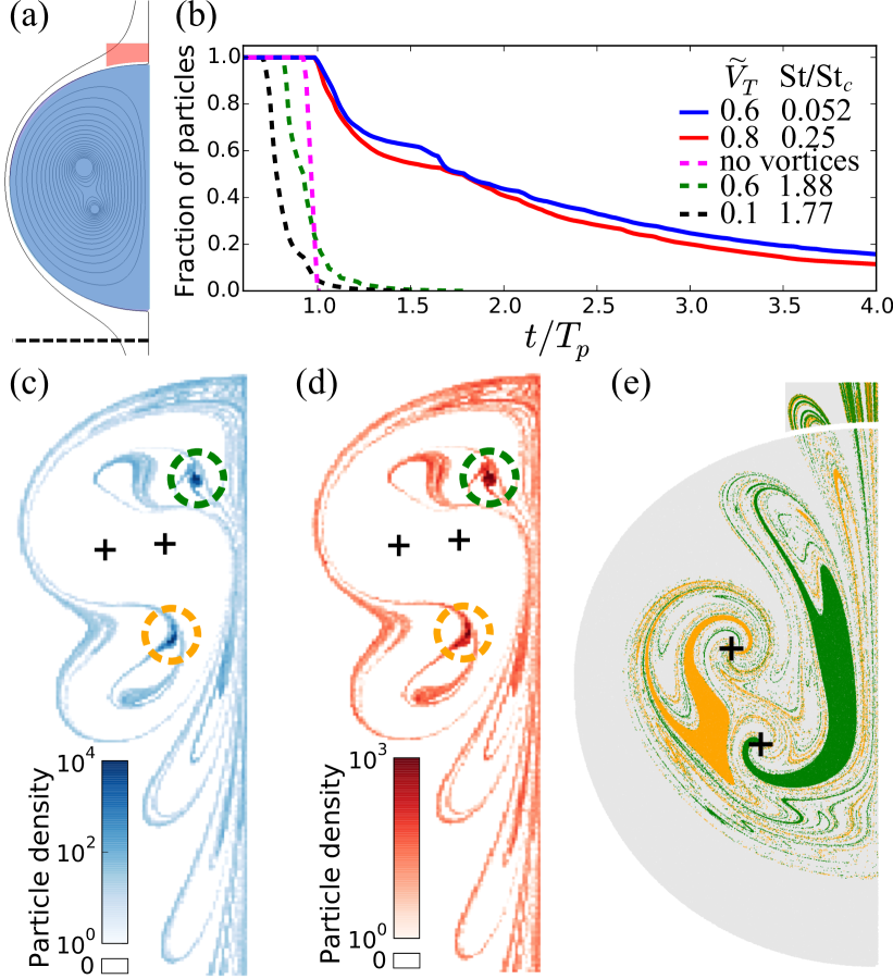
Figure 5: Particle levitation for Navier-Stokes simulations of co-rotating vortices. (a) Initial positions of uniformly distributed particles with zero initial velocity in the open (red) and closed (blue) flow. (b) Fraction of particles from the open flow remaining above a threshold [dashed line in (a)] as a function of time in units of $T_{p}$ (the maximum particle residence time in the absence of vortices). The various choices of $\widetilde{V}_{T}$ and ${\rm St}$ represent scenarios in which: particles are levitated by attracting points (solid lines), particles do not cross into the closed flow region (dashed black), no attracting point are present (dashed green), and vortices are absent (dashed magenta). (c, d) Density plots for particles from the closed (c) and open (d) flows at $t/T_{p}=3.7$ for one choice of parameters in (b) (solid red); dashed circles mark the positions of the attracting points. (e) Section of the attraction basins: initial conditions of particles inside dashed circles of corresponding colors in (c) and (d). The flow parameters are $\gamma=0.7$, $\varepsilon=0.375$, and Reynolds number $Re=4,000$.

To verify the significance of our predictions for more realistic flows, we have simulated viscous flow solutions of the Navier-Stokes equations in the setup of Fig. 1. As shown in Fig. 5, for ${\rm St}<{\rm St}_{c}$, particles with initial positions in both the closed flow [5(a, c)] and open flow [5(a, d)] are captured and levitated by attracting points in the vicinity of the vortices. The main difference from the case of idealized potential flows considered above is that levitation is not permanent in viscous flows since the vortices eventually coalesce. For the conditions considered in Fig. 5, which corresponds to approximately 15 turnover times before vortex merging, particles from the open flow are accelerated downward by vortices alone but, when capture occurs, up to $20\%$ of the particles are levitated by the vortices until they merge [dashed versus continuous lines in Fig. 5(b)]. A partial view of the basins of attraction [Fig.  5(e)] provides further insight into the initial conditions of the particles that can be levitated by this mechanism. Simulations were performed using OpenFOAM. [46] For more details and simulation movies, we refer to the supplementary material.

Our demonstration that heavy particles can be levitated shows that they can be transported in any direction relative to the asymptotic flow and gravity. Exploring this effect in more complex problems (possibly involving non-laminar flows), such as the air-transport of water droplets and aerosols, [47, 49, 48] the resuspension of sediments by coherent vortical structures, [50, 51] and industrial applications for particle sorting, [22, 21] are among the questions of great interest for future research.

Supplementary Material

The supplementary material includes the components of the streamfunction in Eq. (2), analysis of the attracting points, additional details on the Melnikov function calculation and viscous flow simulations, Supplementary Figures for viscous flows, and Supplementary Movies showing animated versions of the dynamics in Fig. 5.

Supplementary Material

Levitation of heavy particles against gravity in asymptotically downward flows
Jean-Régis Angilella, Daniel J. Case, and Adilson E. Motter

Components of the Streamfunction

The components $\psi_{0}$, $\psi_{2c}$, and $\psi_{2s}$ of the steamfunction in Eq. (2) of the main text read

$$\psi_{0}(\mathbf{r}) = \;\;\;\ln\frac{[z^{2}+(y-1)^{2}]^{2}}{[z^{2}+(y+1)^{2}]^{2}}+2y,$$ (S1)

$$\psi_{2c}(\mathbf{r}) = -8y\,{\frac{\left[3\,{z}^{4}-\left(-1+{y}^{2}\right)^{2}+2\,{z}^{2}\left(1+{y}^{2}\right)\right]}{\left[{z}^{2}+\left(1+y\right)^{2}\right]^{2}\left[{z}^{2}+\left(1-y\right)^{2}\right]^{2}}},$$ (S2)

$$\psi_{2s}(\mathbf{r}) = -8yz\,{\frac{\left[-3+{z}^{4}+2\,{y}^{2}+{y}^{4}+2\,{z}^{2}\left(-1+{y}^{2}\right)\right]}{\left[{z}^{2}+\left(1+y\right)^{2}\right]^{2}\left[{z}^{2}+\left(1-y\right)^{2}\right]^{2}}},$$ (S3)

where $\mathbf{r}=(y,z)$ (as indicated in Fig. 1).

Dynamics Near the Attracting Points

To prove the existence and stability of attracting points when gravity is present, we focus on one vortex pair, say $(A,B)$. The pair $(A^{\prime},B^{\prime})$ is assumed to be far from $(A,B)$ so that, to leading order, the angular velocity is $\Omega_{0}$ and the translational velocity of point $I$ is $w_{0}$. We consider the motion of heavy particles in the reference frame rotating at constant velocity $\Omega_{0}$, and translating at constant vertical speed $w_{0}$. We also non-dimensionalize the variables using time and length scales relevant for the dynamics near the vortices: $1/\Omega_{0}$ for times and $d_{0}$ for lengths. These units will be called “internal units” in the following and should not be confused with the “external units” $2L_{0}/w_{0}$ and $L_{0}$ used in the main text to investigate the dynamics near the separatrix $\Sigma_{p}$. In addition, we use the rotating Cartesian coordinates $(I;X,Y,Z)$ where $IX=Ix$ is perpendicular to the plane of the flow, and $IY$ and $IZ$ coincide with $Iy$ and $Iz$ at the initial time. Using $\hat{\mathbf{X}}$, $\hat{\mathbf{Y}}$, and $\hat{\mathbf{Z}}$ to denote the unit vectors in the coordinate directions, the unit vector in the direction of gravity reads $\hat{\mathbf{g}}=-\hat{\mathbf{Y}}\sin t-\hat{\mathbf{Z}}\cos t$.

In this new frame, the non-dimensional equation of motion for heavy particles in the internal system of units is

$$\ddot{\mathbf{R}}=\frac{1}{\mbox{St}}\big{(}\mathbf{W}-\dot{\mathbf{R}}\big{)}+\frac{V_{T}}{\mbox{St}}\hat{\mathbf{g}}+\mathbf{R}-2\hat{\mathbf{X}}\times\dot{\mathbf{R}},$$ (S4)

where ${\mathbf{R}}$ is the particle position and $\mathbf{W}$ is the fluid velocity field (in this frame). The last two terms are the centrifugal and Coriolis forces, respectively. Because particles are much heavier than the fluid, forces proportional to the mass of the displaced fluid, like the Archimedes force and the opposite of the Coriolis and centrifugal forces acting on the fluid, have been neglected. Also, St=$\Omega_{0}\tau_{p}$ is the Stokes number already introduced in the main text, $V_{T}=g\tau_{p}/\Omega_{0}d_{0}$ is the non-dimensional settling velocity in still fluid, and the ratio $V_{T}/$St is the inverse Froude number. The Stokes number (St) and non-dimensional settling velocity ($V_{T}$) introduced with the internal units are related to the external ones by

$$\widetilde{\mbox{St}}=\varepsilon^{2}\mbox{St},\quad\mbox{and}\quad\widetilde{V}_{T}=V_{T}/\varepsilon,$$ (S5)

where $\widetilde{\mbox{St}}\ll 1$, $\mbox{St}=O(1)$, $\widetilde{V}_{T}=O(1)$, and $V_{T}\ll 1$. Therefore, gravitational settling is weak in the internal dynamics (near the vortices) and stronger in the external one (near the separatrix $\Sigma_{p}$). In contrast, particle inertia effects are weak in the external dynamics (which favors the crossing of $\Sigma_{p}$) and stronger near the vortices (which favors capture by attracting points).

To order $\varepsilon^{2}$, the fluid velocity field is

$$\mathbf{W}=\mathbf{W}_{0}(\mathbf{R},\gamma)+\varepsilon^{2}\big{[}\mathbf{W}_{2c}(\mathbf{R},\gamma)\cos 2t+\mathbf{W}_{2s}(\mathbf{R},\gamma)\sin 2t\big{]},$$ (S6)

where the leading order is the relative velocity field induced by an isolated vortex pair with vortex strength ratio $\gamma$ (see, e.g., Ref. [1]) and the velocity fields $\mathbf{W}_{2c}$ and $\mathbf{W}_{2s}$ account for the effect of the vertical wall (the symmetry axis $Oz$ separating $AB$ and $A^{\prime}B^{\prime}$). In the limit of small $\varepsilon$ the wall causes each vortex pair to stretch and compress twice each revolution. That is why, in this frame and system of units, the perturbation terms are proportional to $\cos 2t$ and $\sin 2t$.

To analyze the stability of equilibrium points, we follow the procedure employed by IJzermans and Hagmeijer in Ref. [2], and set

$$\mathbf{R}(t)=\mathbf{R}_{eq}+\mathbf{h}(t),$$ (S7)

where $\mathbf{R}_{eq}$ denotes any one of the equilibrium points in the rotating frame in the absence of both wall and gravity (the existence of these points, when neither wall nor gravity is present, has been proven in Ref. [3] for identical vortices and in Ref. [1] for unequal vortices). In particular, $\mathbf{R}_{eq}$ is any solution of $\mathbf{W}_{0}(\mathbf{R}_{eq})/\mbox{St}+\mathbf{R}_{eq}=\mathbf{0}$, which reflects the balance between inward drag and the centrifugal force at the equilibrium point. In Eq. (S7), $\mathbf{h}=\mathbf{h}(t)$ represents the perturbation accounting for the effect of gravity and the wall. Using this decomposition in Eq. (S4), and neglecting the quadratic terms in $\mathbf{h}$, we obtain

$$\ddot{\mathbf{h}}=\frac{1}{\mbox{St}}\Big{\{}({\text{D}}\mathbf{W}_{0}^{eq})\,\mathbf{h}+\varepsilon^{2}\Big{[}\mathbf{W}_{2c}(\mathbf{R}_{eq},\gamma)\cos 2t+\mathbf{W}_{2s}(\mathbf{R}_{eq},\gamma)\sin 2t$$

$$-\widetilde{V}_{T}(\hat{\mathbf{Y}}\sin t+\hat{\mathbf{Z}}\cos t)\Big{]}-\dot{\mathbf{h}}\Big{\}}+{\mathbf{h}}-2\hat{\mathbf{X}}\times\dot{\mathbf{h}}\,,$$ (S8)

where ${\text{D}}{\mathbf{f}}$ is used to denote the Jacobian matrix of ${\mathbf{f}}$ and ${\text{D}}\mathbf{W}_{0}^{eq}={\text{D}}\mathbf{W}_{0}|_{\mathbf{R}_{eq}}$. The general solution of this non-homogeneous linear equation is the sum of a particular solution $\mathbf{h}_{a}(t)$ and the solution $\mathbf{h}_{b}(t)$ of the homogeneous part of the equation.

The homogeneous equation corresponds exactly to the case in which both gravity and the wall are absent. Focusing on equilibrium points $\mathbf{R}_{eq}$ that (in the absence of gravity and the wall) are asymptotically stable, we have $\mathbf{h}_{b}(t)\to 0$ as $t\to+\infty$. Provided the internal Stokes number is not too large, as considered here, there are either one or two such stable points when neither gravity nor the wall is present [1]; from here on we consider only these equilibria and show that they are converted into time-dependent attracting points when the effect of gravity and/or the wall are significant.

The particular solution can be sought in the form of a combination of two Fourier modes:

$$\mathbf{h}_{a}(t)=\sum_{n=1,2}(\mathbf{p}_{n}\cos nt+\mathbf{q}_{n}\sin nt),$$ (S9)

where the amplitudes $\mathbf{p}_{n}$ and $\mathbf{q}_{n}$ are given by a set of linear equations,

$$\mathbf{L}_{1}\mathbf{p}_{1}-\mathbf{M}_{1}\mathbf{q}_{1} = \varepsilon^{2}\frac{\widetilde{V}_{T}}{\mbox{St}}\hat{\mathbf{Z}},$$ (S10)

$$\mathbf{L}_{1}\mathbf{q}_{1}+\mathbf{M}_{1}\mathbf{p}_{1} = \varepsilon^{2}\frac{\widetilde{V}_{T}}{\mbox{St}}\hat{\mathbf{Y}},$$ (S11)

$$\mathbf{L}_{2}\mathbf{p}_{2}-\mathbf{M}_{2}\mathbf{q}_{2} = -\frac{\varepsilon^{2}}{\mbox{St}}\mathbf{W}_{2c}(\mathbf{R}_{eq},\gamma),$$ (S12)

$$\mathbf{L}_{2}\mathbf{q}_{2}+\mathbf{M}_{2}\mathbf{p}_{2} = -\frac{\varepsilon^{2}}{\mbox{St}}\mathbf{W}_{2s}(\mathbf{R}_{eq},\gamma),$$ (S13)

for $\mathbf{L}_{1}=\frac{\mbox{1}}{\mbox{St}}{\text{D}}\mathbf{W}_{0}^{eq}+2\mathbf{I}$, $\mathbf{M}_{1}=\frac{\mbox{1}}{\mbox{St}}\mathbf{I}+2\mathbf{A}$, $\mathbf{L}_{2}=\mathbf{L}_{1}+3\mathbf{I}$, $\mathbf{M}_{2}=2\mathbf{M}_{1}$, and matrix $\mathbf{A}$ representing a rotation of $\pi/2$ around $\hat{\mathbf{X}}$. The matrices $\mathbf{M}_{1}$ and $\mathbf{M}_{2}$ are invertible—it can be checked that their determinants are nonzero irrespective of St. The matrix $\mathbf{L}_{1}$ is also invertible since its eigenvalues are $\lambda_{i}=2+\mu_{i}/\mbox{St}$ ($i=1,2$), where $\mu_{i}$’s are the eigenvalues of the matrix ${\text{D}}\mathbf{W}_{0}^{eq}$, which are known to have non-zero imaginary parts. Finally, a similar argument can be used to show that the matrix $\mathbf{L}_{2}$ is also invertible. Thus, after some elementary algebra, we are led to

$$\big{(}\mathbf{M}_{1}^{-1}\mathbf{L}_{1}+\mathbf{L}_{1}^{-1}\mathbf{M}_{1}\big{)}\mathbf{p}_{1}=\varepsilon^{2}\frac{\widetilde{V}_{T}}{\mbox{St}}\big{(}\mathbf{L}_{1}^{-1}\hat{\mathbf{Y}}+\mathbf{M}_{1}^{-1}\hat{\mathbf{Z}}\big{)}.$$ (S14)

By solving this last system we obtain the amplitude $\mathbf{p}_{1}$. The other amplitudes $\mathbf{p}_{n}$ and $\mathbf{q}_{n}$ can be obtained in a similar way, so that the periodic solution $\mathbf{h}_{a}(t)$ in Eq. (S9) exists and is uniquely defined.

We therefore conclude that, for sufficiently small $\varepsilon\ll 1$, the trajectories of inertial particles in the presence of gravity and the wall converge to some periodic orbit in an $\varepsilon^{2}$-neighborhood of the equilibrium point $\mathbf{R}_{eq}$ of the unperturbed system.

Calculation of the Melnikov Function

The variation of the undisturbed Hamiltonian $H=\psi_{p}(\mathbf{r}(t))$ along the disturbed trajectory $\mathbf{r}(t)$ between the discrete times $\tau_{2n}$ and $\tau_{2n+1}$ is [4, 5]

$$H_{n+1}-H_{n}=\int_{\tau_{2n}}^{\tau_{2n+1}}\frac{d}{dt}\psi_{p}(\mathbf{r}(t))\,dt=\int_{\tau_{2n}}^{\tau_{2n+1}}\nabla\psi_{p}({\mathbf{r}}(t))\cdot\frac{d{\mathbf{r}}(t)}{dt}\,dt.$$ (S15)

Assuming the trajectory is close to the separatrix $\Sigma_{p}$, we write $\mathbf{r}(t)\simeq\mathbf{q}(t-t_{n})$, where $\mathbf{q}(t)$ is a trajectory on $\Sigma_{p}$. Therefore it satisfies $\dot{\mathbf{q}}=\mathbf{v}_{0}(\mathbf{q})$, $\mathbf{q}(-\infty)=S_{1}$, and $\mathbf{q}(+\infty)=S_{2}$, where the $z$-coordinates of $S_{1}$ and $S_{2}$ are given by $z=\pm\big{[}(6-\widetilde{V}_{T})/(2+\widetilde{V}_{T})\big{]}^{1/2}$. For convenience, we take the initial condition $\mathbf{q}(0)$ at the intersection between $\Sigma_{p}$ and the axis $Oy$. In addition, we perform the change of variables $t\to t-t_{n}$, and take into account the fact that $\tau_{2n}-t_{n}<0<\tau_{2n+1}-t_{n}$ and that $|\tau_{2n}-t_{n}|\gg 1$ and $|\tau_{2n+1}-t_{n}|\gg 1$ (because the dynamics is very slow near $S_{1}$ and $S_{2}$). The integration interval $[\tau_{2n}-t_{n},\tau_{2n+1}-t_{n}]$ can then be replaced by $[-\infty,+\infty]$, leading to $H_{n+1}-H_{n}=\varepsilon^{2}M(t_{n})$, where $M(t_{n})$ is the Melnikov function,

$$M(t_{n})=\int_{-\infty}^{\infty}\negmedspace\negmedspace\negmedspace\negmedspace{\mathbf{v}}_{0}({\mathbf{q}}(t))\times{\mathbf{v}}_{2}\Big{(}\mathbf{q}(t),\frac{t+t_{n}}{\varepsilon^{2}}\Big{)}\,dt.$$ (S16)

Note that in this equation and others below, the cross products should be interpreted as projected in the $\hat{\mathbf{x}}$ direction.

The unperturbed trajectory ${\mathbf{q}}(t)$ cannot be obtained analytically for arbitrary $\widetilde{V}_{T}$. We therefore approximate it by assuming that $\widetilde{V}_{T}$, though larger than the internal non-dimensional velocity $V_{T}$, is sufficiently smaller than unity that it allows us to write ${\mathbf{q}}(t)={\mathbf{q}}_{0}(t)+\widetilde{V}_{T}\,{\mathbf{q}}_{1}(t)+O(\widetilde{V}_{T}^{2})$, where the functions ${\mathbf{q}}_{0}(t)$ and ${\mathbf{q}}_{1}(t)$ are determined numerically. Setting $\mathbf{U}_{2}=\mathbf{u}_{2}-\mbox{St}\,\partial\mathbf{u}_{2}/\partial\tau$, after some algebra the Melnikov function reads

$$M(t_{n})=I_{1}+I_{2}+I_{3}+O(\widetilde{V}_{T}^{2})+O(\widetilde{V}_{T}\mbox{St}),$$ (S17)

where

$$I_{1}=\int_{-\infty}^{\infty}\negmedspace\negmedspace\negmedspace\negmedspace\dot{\mathbf{q}}_{0}(t)\times{\mathbf{U}}_{2}\Big{(}\mathbf{q}_{0}(t),\frac{t+t_{n}}{\varepsilon^{2}}\Big{)}\,dt-\mbox{St}\int_{-\infty}^{\infty}\negmedspace\negmedspace\negmedspace\negmedspace\dot{\mathbf{q}}_{0}(t)\times\ddot{\mathbf{q}}_{0}(t)\,dt,$$ (S18)

$$I_{2}=\widetilde{V}_{T}\int_{-\infty}^{\infty}\negmedspace\negmedspace\negmedspace\negmedspace\dot{\mathbf{q}}_{1}(t)\times\mathbf{U}_{2}\Big{(}\mathbf{q}_{0},\frac{t+t_{n}}{\varepsilon^{2}}\Big{)}\,dt,$$ (S19)

$$I_{3}=\widetilde{V}_{T}\int_{-\infty}^{\infty}\negmedspace\negmedspace\negmedspace\negmedspace\dot{\mathbf{q}}_{0}(t)\times\Big{(}({\text{D}}\mathbf{U}_{2})\,\mathbf{q}_{1}(t)\Big{)}\,dt.$$ (S20)

By expanding the sines and cosines appearing in $I_{1}$ and assigning zero to the integrals of odd functions of $t$, we obtain

$$I_{1}=\frac{4\gamma}{(1+\gamma)^{2}}a(\varepsilon)\Big{(}\sin\frac{2t_{n}}{\varepsilon^{2}}-2\mbox{St}\cos\frac{2t_{n}}{\varepsilon^{2}}\Big{)}-m\,\mbox{St},$$ (S21)

where the multiplicative coefficient $a(\varepsilon)$ depends only on $\varepsilon$,

$$a(\varepsilon)=\int_{-\infty}^{\infty}\negmedspace\negmedspace\negmedspace\negmedspace\dot{\mathbf{q}}_{0}(t)\times\Big{[}{\mathbf{u}}_{2s}(\mathbf{q}_{0}(t))\cos\frac{2t}{\varepsilon^{2}}-{\mathbf{u}}_{2c}(\mathbf{q}_{0}(t))\sin\frac{2t}{\varepsilon^{2}}\Big{]}\,dt,$$ (S22)

and $m$ is a constant,

$$m=\int_{-\infty}^{\infty}\negmedspace\negmedspace\negmedspace\negmedspace\dot{\mathbf{q}}_{0}(t)\times\ddot{\mathbf{q}}_{0}(t)\,dt.$$ (S23)

The velocity fields $\mathbf{u}_{2c}$ and $\mathbf{u}_{2s}$ correspond to the streamfunctions $\psi_{2c}$ and $\psi_{2s}$ respectively.

The constant $m$ is computed numerically once $\mathbf{q}_{0}(t)$ has been determined, resulting in $m\simeq 30.4$. The function $a(\varepsilon)$ is also computed numerically, and then fitted with an exponential-rational function of the form

$$a(\varepsilon)=\frac{e^{-\alpha_{e}/\varepsilon^{2}}}{\varepsilon^{2}}\big{(}\alpha_{0}+\alpha_{2}\varepsilon^{2}+\alpha_{4}\varepsilon^{4}\big{)},$$ (S24)

where the $\alpha_{i}$’s are obtained using a least-square algorithm. The resulting constants are $\alpha_{e}\simeq 0.60$, $\alpha_{0}\simeq 16.5$, $\alpha_{2}\simeq-9.5$, and $\alpha_{4}\simeq-51.5$. Applying the same treatment to the integrals $I_{2}$ and $I_{3}$, we obtain

$$I_{2}+I_{3}=\frac{4\gamma}{(1+\gamma)^{2}}\,\widetilde{V}_{T}\big{[}b_{2}(\varepsilon)+b_{3}(\varepsilon)\big{]}\Big{(}\sin\frac{2t_{n}}{\varepsilon^{2}}-2\mbox{St}\cos\frac{2t_{n}}{\varepsilon^{2}}\Big{)},$$ (S25)

where

$$b_{2}(\varepsilon)=\int_{-\infty}^{\infty}\negmedspace\negmedspace\negmedspace\negmedspace\dot{\mathbf{q}}_{1}(t)\times\Big{[}{\mathbf{u}}_{2s}(\mathbf{q}_{0}(t))\cos\frac{2t}{\varepsilon^{2}}-{\mathbf{u}}_{2c}(\mathbf{q}_{0}(t))\sin\frac{2t}{\varepsilon^{2}}\Big{]}\,dt,$$ (S26)

$$b_{3}(\varepsilon)=\int_{-\infty}^{\infty}\negmedspace\negmedspace\negmedspace\negmedspace\dot{\mathbf{q}}_{0}(t)\times\Big{[}({\text{D}}{\mathbf{u}}_{2s})\,\mathbf{q}_{1}(t)\,\cos\frac{2t}{\varepsilon^{2}}-({\text{D}}{\mathbf{u}}_{2c})\,\mathbf{q}_{1}(t)\,\sin\frac{2t}{\varepsilon^{2}}\Big{]}\,dt.$$ (S27)

Both $b_{2}$ and $b_{3}$ depend only on $\varepsilon$ and are computed numerically once ${\mathbf{q}}_{0}(t)$ and ${\mathbf{q}}_{1}(t)$ have been determined. The sum $b_{2}(\varepsilon)+b_{3}(\varepsilon)$, denoted $b(\varepsilon)$ in the main text, is fitted with an exponential-rational function of same form as the one used for $a(\varepsilon)$, with the coefficients $\alpha_{i}$’s replaced by $\beta_{i}$’s: $\beta_{e}\simeq 0.60$, $\beta_{0}\simeq 174.6$, $\beta_{2}\simeq-1120.6$, and $\beta_{4}\simeq 1972.0$.

Navier-Stokes Simulations of Viscous Flows

The computations in Figs. 2-4 (main text) were performed assuming idealized inviscid flows (exact solutions of the Euler equations). For moderate Reynolds number, viscosity is expected to have significant effects on the flow, as viscous diffusion causes the size of the vortex cores to expand over time. Once the radius of either core becomes comparable to the distance between the vortices, vortex merging occurs and any attractors of the particle dynamics vanish. We performed simulations solving the two-dimensional Navier-Stokes equations with a viscous working fluid to determine whether heavy-particle levitation could be observed prior to the eventual coalescence of the vortices. The initial velocity field of the fluid consisted of the superposition of a uniform downward flow (in the direction of gravity) with a velocity magnitude of $0.625w_{0}$ relative to the laboratory reference frame and two pairs of co-rotating Lamb-Oseen vortices with inter-vortex distance $2d_{0}$ as in the setup of Fig. 1 (main text). The Reynolds number of the flow, $Re=\Omega_{0}{d_{0}}^{2}/\nu$, where $\nu$ is the dynamic viscosity of the fluid, was set to be $4,000$ in all simulations we report. For these conditions, in each run of our simulations we released $100,000$ particles from the closed flow and $50,000$ from the open flow with zero initial velocity, as defined in Fig. 5(a) (main text). After simulating many combinations of $\widetilde{V}_{T}$ and $\widetilde{\mbox{St}}$, we observed the following scenarios: for ${\mbox{St}}/{\mbox{St}}_{c}>1$ either no attracting points exist or they exist but no particles from the open flow are captured by them; for ${\mbox{St}}/{\mbox{St}}_{c}<1$ attracting points exist and particles from the open flow are captured and levitated by them.

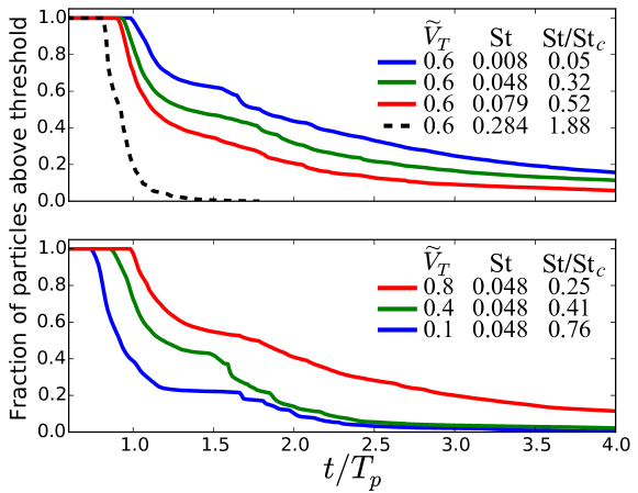
Figure S1: Fraction of particles from the open flow that remain above the threshold marked in Fig. 5(a) in the main text as function of time, for $\gamma=0.7$ and $\varepsilon=0.375$. The different curves correspond to (a) different choices of St for $\widetilde{V}_{T}=0.6$ and (b) different choices of $\widetilde{V}_{T}$ for ${\mbox{St}}=0.048$. The fraction of particles levitated for a long period increases as St is decreased and as $\widetilde{V}_{T}$ is (and hence gravity) increased, which parallels the dependence of $\mbox{St}_{c}$ in our theory based on potential flows.

To quantify the levitation mechanism for particles from the open flow, we calculate the fraction of particles released in the open flow that remain above a threshold as a function of time. We set the threshold to a distance $2.4L_{0}$ downstream from the initial center of vorticity $I$, which lies right below the closed flow separatrix so that any particle that falls below this threshold will not be pulled back upstream. This fraction is shown in Fig. S1, illustrating the different scenarios mentioned above, where time is represented in units of the maximum time $T_{p}$ a particle with the given initial conditions would remain above threshold in the the same flow without vortices. We define the levitation period to be the time $t-T_{p}$ the particle remains above this threshold. For example, for $\widetilde{V}_{T}=0.6$ and ${\mbox{St}}/{\mbox{St}}_{c}=0.05$ particles from the open flow approach the attracting points and nearly $20\%$ of the particles have a levitation period larger than $3T_{p}$. For $\widetilde{V}_{T}=0.6$ and ${\mbox{St}}/{\mbox{St}}_{c}=1.88$, on the other hand, there are no attractors in the vicinity of the vortices and the levitation period is close to zero for most particles. We also observe that for a fixed value of St, increasing $\widetilde{V}_{T}$ can increase the fraction of particles above the threshold at all times, which is counter-intuitive but consistent with our analytical results for potential flow, where stronger gravity is observed to enhance the levitation effect.

Simulations were performed with OpenFOAM (version $2.2$) using the PISO algorithm in solving for the flow field. [6] The particle motion was calculated with Lagrangian particle tracking with one-way coupling of the particles to the fluid.

Animated Visualization of Navier-Stokes Simulations

Supplementary Movies 1, 2, 3, and 4 show the particle and fluid dynamics for the scenarios of Navier-Stokes simulations exemplified in Fig. 5(b) (main text). Each movie corresponds to a different choice of $\widetilde{V}_{T}$ and St for the same flow. Figure S2 shows snapshots for each movie, with the corresponding parameters indicated in the caption.

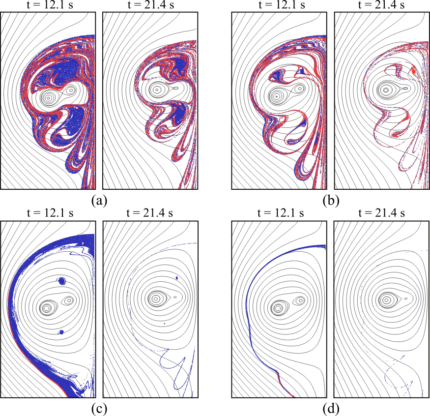
Figure S2: Early and late snapshots of the Supplementary Movies showing the advection of heavy particles by the viscous flow considered in Fig. 5(b) (main text). (a) Movie 1: $\widetilde{V}_{T}=0.6$ and ${\mbox{St}}/{\mbox{St}}_{c}=0.052$, for which attracting points exist and particles from both the closed and the open flow are levitated. (b) Movie 2: $\widetilde{V}_{T}=0.8$ and ${\mbox{St}}/{\mbox{St}}_{c}=0.25$, scenario similar to (c) for a different parameter choice. (c) Movie 3: $\widetilde{V}_{T}=0.1$ and ${\mbox{St}}/{\mbox{St}}_{c}=1.77$, for which attracting points exist and levitate particles from the closed flow, but no particles from the open flow can approach them. (d) Movie 4: $\widetilde{V}_{T}=0.6$ and ${\mbox{St}}/{\mbox{St}}_{c}=1.88$, for which no attracting points exist and all particles are centrifuged away from the vortices. In all panels, blue (red) represent particles from the closed (open) flow, where we choose to show only red in the overlapping areas, and solid curves mark streamlines of the flow.

Supplementary References

References

-
[1]
T. Nizkaya, J. R. Angilella, and M. Buès,
Note on dust trapping in vortex pairs with unequal strengths,
Phys. Fluids 22, 113301 (2010).
-
[2]
R. H. A. IJzermans and R. Hagmeijer,
Accumulation of heavy particles in N-vortex flow on a disk,
Phys. Fluids 18, 063601 (2006).
-
[3]
J. R. Angilella,
Dust trapping in vortex pairs,
Physica (Amsterdam) 239D, 1789 (2010).
-
[4]
B. V. Chirikov,
A universal instability of many-dimensional oscillator systems,
Phys. Rep. 52, 263 (1979).
-
[5]
L. Kuznetsov and G. M. Zaslavsky,
Hidden renormalization group for the near separatrix Hamiltonian dynamics,
Phys. Rep. 288, 457 (1997).
-
[6]
R. I. Issa,
Solution of the implicitly discretised fluid flow equations by operator-splitting,
J. Comput. Phys. 62, 40 (1986).