Description of the evolution of inhomogeneities on a Dark Matter halo with the Vlasov equation

Abstract

We use a direct numerical integration of the Vlasov equation in spherical symmetry with a background gravitational potential to determine the evolution of a collection of particles in different models of a galactic halo. Such a collection is assumed to represent a dark matter inhomogeneity which reaches a stationary state determined by the virialization of the system. We describe some features of the stationary states and, by using several halo models, obtain distinctive signatures for the evolution of the inhomogeneities in each of the models.

I Introduction

The nature of dark matter remains one of the most puzzling questions in modern cosmology. Its assumed that elementary particles could be the constituents of dark matter for which there have been several experimental attempts to perform a direct detection of such dark matter particle, but still a clear evidence for such particles remains absent Undagoitia:2015gya . Examples of these experiments are the Large Underground Xenon (LUX) experiment Akerib:2012ys , the DAMA/Libra experiment Bernabei:2008yh , ZEPLIN experiment Akimov:2006qw , XENON10 experiment Aprile:679A or DAMIC experiment at SNOLAB Barreto:2011zu , Chavarria:2014ika ; Aguilar-Arevalo:2016zop ; Aguilar-Arevalo:2016ndq . Another approach to determine the nature of dark matter is to find specific features in the dynamics of visible matter in the presence of the gravitational potential of a dark matter halo.

Dark matter is usually assumed to be a stable particle with no electric charge, and with a negligible cross-section with baryonic particles. However, it does interact gravitationally with the rest of the matter (in general relativistic terms, dark matter does curve space-time). It is also assumed that dark matter particles only interact with themselves gravitationally, or that at least any non-gravitational self-interaction is very weak. This means that a fluid description of dark matter is not adequate (even though this description may lead to some intuitive properties Barranco:2013wy ). Indeed, the fluid approximation requires that the mean-free path of particles is much smaller than the characteristic size of the system, which clearly does not apply to dark matter particles. One should mention that there are serious proposals that consider that dark matter can be described as an ultra-light scalar field, and such proposals seem to ameliorate some of the problems related with the usual dark matter paradigm (see e.g. Matos:1999et ; Matos:2000xi ; Matos:2003pe ).

If one considers dark matter as a collection of non-interactive particles there are at least two different ways to study their dynamics. The standard approach has been to study them using increasingly sophisticated direct gravitational N-body simulations, with today can use billions of particles Navarro:1995iw ; Harker:2005um . In N-body simulations, each particle represents a very large number of dark matter particles and the interaction between two particles is computed by assuming that they have a finite size and density profile, which leads to an effective softening force at small scales Athanassoula:10.1046 ,Dehnen:10.1046 . In this way, a given density velocity field is represented by a set of particles Hockney:1981csup . For more details on the techniques and status of these simulations one can refer to Bagla:2004au . Another approach is to use a continuum approximation based on kinetic theory and the Boltzmann equation BT2 . In this second approach a collection of particles is described in a collective way by means of a distribution function $f$ defined as a probability density in the so-called phase space, namely the space defined by generalized coordinates and momenta. When the particles are non-interactive, one obtains the homogeneous Boltzmann equation, also known as the Vlasov equation BT2 . Such description is nearly equivalent to the numerical description of dark matter by means of the N-body simulations, although there are conceptual and quantitative differences in the two approaches Colombi:2015eia .

Solutions of the Vlasov equation are frequently not easy to interpret. It is quite easy to solve in general, since by just by expressing the distribution function as a function of conserved quantities we automatically obtain an exact, and stationary, solution Andreasson:2005qy . However, such general solutions often do not have a clear physical interpretation, and can lead to misunderstandings Shapiro:1983du . We have found it productive then, to solve the Vlasov equation dynamically in order to study the evolution in phase space of an initial distribution function, which allows for a more clear physical interpretation. Using this approach, we study the evolution of a spherically symmetric distribution function in different gravitational potentials, which describe several models of dark matter halos. The distribution function is assumed to describe a dark matter inhomogeneity within the dark matter halo. The aim of this work is first to develop a robust numerical integration code for the Vlasov equation, and then use it to test the stability of inhomogeneities in dark mater halos, as well as to obtain non-trivial final stationary states for the initial inhomogeneity.

The paper is organized as follows: In Section II we present a brief review of kinetic theory, introducing the Vlasov equation. In Section III we present four different halo gravitational potentials, and derive a dimensionless Vlasov equation for the corresponding models. In Section IV we describe the code used to perform the numerical simulations of the evolution of the distribution function by means of the Vlasov equation. After that, we present our results for each halo model in Section V. Finally, we discuss our findings in Section VI.

II Kinetic theory and Vlasov equation

II.1 Distribution function in spherical symmetry

The particle distribution function $f$ lives in a higher dimensional phase-space: six dimensional in the case of classical mechanics, and seven dimensional in relativistic physics (down from eight due to the constraint on the magnitude of the momenta, the so-called mass-shell condition $p_{\mu}p^{\mu}=-m^{2}c^{2}$, where $m$ is the particle’s mass and $c$ denotes the speed of light). The general explicit invariant volume element in momentum space in the general relativistic description is

$$d\omega=\frac{d^{3}\,p_{*}}{p^{0}\,\sqrt{-g}}\;,$$ (1)

where $p_{*}$ denotes the covariant momenta, $p_{i}=\partial L/\partial\dot{x}^{i}$, with $L$ the Lagrangian, and where $g$ is the determinant of the spacetime metric. In the Newtonian limit this volume element takes the form

$$d\omega=\frac{d^{3}\,p_{*}}{\sqrt{h}}\;,$$ (2)

where now $h$ is the determinant of the flat metric in the coordinates under consideration, and the momenta $p_{*}$ corresponds to the conjugate momenta. Notice that since in general the volume element in physical space is given by $dV=\sqrt{h}\;d^{3}x$, one finds that the phase space volume element $dVd\omega$ is in fact invariant.

Keeping in the Newtonian limit, when using Cartesian coordinates the invariant volume element in momentum space takes the form $d\omega=dp_{x}dp_{y}dp_{z}$, and when using spherical coordinates it becomes

$$d\omega=\frac{dp_{r}\;dp_{\theta}\;dp_{\varphi}}{r^{2}\sin\theta}\;.$$ (3)

There is in fact another expression that is commonly used for the invariant volume element in momentum space in spherical coordinates, namely $d\omega=p^{2}\sin\theta_{p}\;dp\;d\theta_{p}\;d\varphi_{p}$, where $p$ is the magnitude of the momentum, and $(\theta_{p},\varphi_{p}$) are angles defined in momentum space in the same way as ($\theta$,$\varphi$) are defined in the space sector, so that for example $p_{x}=p\sin\theta_{p}\cos\varphi_{p},p_{y}=p\sin\theta_{p}\sin\varphi_{p},p_{z}=p\cos\theta_{p}$. This volume element can be related to the former expression, Eq. (3), by the Jacobian of the corresponding coordinate transformation Dominguez:2015 ; Jimenez:2016 .

In the following we will consider a stationary background gravitational potential with spherical symmetry, and a distribution function $f(t,x^{i},p_{i})$ that is also spherically symmetric. Moreover, instead of the angular conjugated momenta, $p_{\theta},p_{\varphi}$, we will use the conserved total angular momentum squared, $L^{2}$, and an auxiliary angle, $\psi$:

$$L^{2} = p_{\theta}^{2}+\frac{p_{\varphi}^{2}}{\sin^{2}\theta},$$ (4)

$$\psi = \arctan\left(\frac{p_{\theta}\sin\theta}{p_{\varphi}}\right),$$ (5)

so that the invariant volume element, Eq. (1), takes the form

$$d\omega=\frac{1}{2r^{2}}\;dp_{r}\,dL^{2}\,d\psi=\frac{L}{r^{2}}\;dp_{r}\,dL\,d\psi\;.$$ (6)

Finally, since we will be working with spherical symmetry, the distribution function will have no dependence on $\psi$.

We will therefore integrate over $\psi$ so the volume element used for this work will have the final form

$$d\bar{\omega}=\int\left(d\omega\right)\;d\psi=\frac{\pi}{r^{2}}\;dp_{r}\,dL^{2}=\frac{2\pi L}{r^{2}}\;dp_{r}\,dL\;.$$ (7)

In spherical symmetry the distribution function will have the form $f=f(t,r,p_{r},L)$. This implies that in the case of spherical symmetry, the phase space is effectively tri-dimensional. At this point it is important to mention a couple of details about this distribution function. First, even though we are in spherical symmetry, the individual particles can have non-trivial angular momentum. The spherical symmetry will be maintained as long as at any given point in space with a certain radial distance $r$ from the origin, the tangential velocities of the particles are distributed uniformly in every possible direction. Second, notice that since $f$ depends on the angular momentum $L$, and this is defined through (4), the distribution $f$ when rewritten in terms of $(p_{r},p_{\theta},p_{\varphi})$ will in fact depend on the angle $\theta$. This might seem odd since after all we are in spherical symmetry, but as we will see below this dependence in fact cancels out in the Vlasov equation.

We can now define the particle density $\rho_{f}$ in physical space, the momentum density $j_{f}$, and the mean value over momentum space of an arbitrary function $g$, will take the form

$$\rho_{f}(t,r) \equiv \int f(t,r,p_{r},L)\;d\bar{\omega}=\frac{2\pi}{r^{2}}\int f(t,r,p_{r},L)\;L\;dp_{r}\;dL\;,$$ (8)

$$j_{f}(t,r) \equiv \int p_{r}f(t,r,p_{r},L)\;d\bar{\omega}=\frac{2\pi}{r^{2}}\int p_{r}f(t,r,p_{r},L)\;L\;dp_{r}\;dL\;,$$ (9)

$$\bar{g}(t,r) \equiv \int gf(t,r,p_{r},L)\;d\bar{\omega}=\frac{2\pi}{r^{2}}\int gf(t,r,p_{r},L)\;L\,dp_{r}\,dL\;.$$ (10)

The total number of particles can then be defined as

$$N=\int f\;dVd\bar{\omega}=8\pi^{2}\int fL\;drdp_{r}dL=4\pi\int\rho_{f}r^{2}dr\;.$$ (11)

One can also define of the average value of a given physical quantity over the complete phase space as

$$\left<g\right>(t)\equiv 8\pi^{2}\int gf(t,r,p_{r},L)\;L\;dp_{r}\;dL\;dr=4\pi\int\bar{g}(t,r)\;r^{2}dr\;.$$ (12)

As a further simplifying assumption, we will also assume that all the particles have the same conserved angular momentum $L_{0}$, so that, using a delta function, we can write $f(t,r,p_{r},L)=F(t,r,p_{r})\delta(L-L_{0})$, obtaining

$$\rho_{f}(t,r) = \frac{2\pi L_{0}}{r^{2}}\int F(t,r,p_{r};L_{0})\;dp_{r}\;,$$ (13)

$$j_{f}(t,r) = \frac{2\pi L_{0}}{r^{2}}\int p_{r}F(t,r,p_{r};L_{0})\;dp_{r}\;,$$ (14)

$$\bar{g}(t,r) = \frac{2\pi L_{0}}{r^{2}}\int gF(t,r,p_{r};L_{0})\;dp_{r}\;,$$ (15)

$$\left<g\right>(t) = 8\pi^{2}L_{0}\int gF(t,r,p_{r};L_{0})\;dp_{r}\;dr\;,$$ (16)

$$N = 8\pi^{2}L_{0}\int F(t,r,p_{r};L_{0})\;drdp_{r}\;.$$ (17)

One should also mention the fact that for the particular case when the motion is purely radial and the angular momentum is zero, $L_{0}=0$, the above equations are in fact not correct and the derivation has to be made again from the top (a naive application of these expressions would seem to indicate that all the integrals above vanish). That is, we have to begin with a Dirac delta dependence of the distribution function in the angular momenta

$$f(t,r,p_{r},p_{\theta},p_{\varphi})=F(t,r,p_{r})\;\delta(p_{\theta})\;\delta(p_{\varphi}/\sin\theta)$$ (18)

Transforming the Dirac deltas from coordinates ($p_{\theta}$,$p_{\varphi}$) to the new coordinates ($L$,$\psi$) yields

$$\delta(p_{\theta})\;\delta(p_{\varphi}/\sin\theta)=\frac{1}{L}\;\delta(L)\;\delta(\psi)\;.$$

So that the expressions for the density, current, mean value and average in the case of zero angular momentum become

$$\rho_{f}(t,r) = \frac{1}{r^{2}}\int F(t,r,p_{r})\;dp_{r}\;,$$ (19)

$$j_{f}(t,r) = \frac{1}{r^{2}}\int p_{r}\;F(t,r,p_{r})\;dp_{r}\;,$$ (20)

$$\bar{g}(t,r) = \frac{1}{r^{2}}\int g\;F(t,r,p_{r})\;dp_{r}\;,$$ (21)

$$\left<g\right>(t) = 4\pi\int g\;F(t,r,p_{r})\;dp_{r}\;dr\;,$$ (22)

$$N = 4\pi\int F(t,r,p_{r})\;dp_{r}\;dr\;.$$ (23)

II.2 Vlasov equation

Let us now consider the Vlasov equation. In the general case, the collisionless Boltzmann equation, also known as the Vlasov equation, has the form

$$\frac{\partial f}{\partial t}+\frac{dx^{i}}{dt}\;\frac{\partial f}{\partial x^{i}}+\frac{dp^{i}}{dt}\;\frac{\partial f}{\partial p^{i}}=0\;.$$ (24)

In spherical symmetry, and with the definitions given above, this reduces to

$$\frac{\partial f}{\partial t}=-\frac{p_{r}}{m}\;\frac{\partial f}{\partial r}-\frac{p_{\theta}}{mr^{2}}\;\frac{\partial f}{\partial\theta}-\dot{p}_{r}\;\frac{\partial f}{\partial p_{r}}-\dot{p}_{\theta}\;\frac{\partial f}{\partial p_{\theta}}\;.$$ (25)

Notice that, as mentioned before, even in spherical symmetry the distribution function has a dependency on $\theta$ when written in terms of the conjugate momenta.

Now, for a central potential $\Phi(r)$, the equations of motion are

$$\dot{p}_{r} = -\frac{\partial{\cal H}}{\partial r}=-\frac{\partial\Phi}{\partial r}+\frac{L^{2}}{mr^{3}}\;,$$ (26)

$$\dot{p}_{\theta} = -\frac{\partial{\cal H}}{\partial\theta}=\frac{{p_{\varphi}}^{2}\cos\theta}{mr^{2}\sin^{3}\theta}\;,$$ (27)

where ${\cal H}$ is the Hamiltonian of the system. This implies that

$$\frac{p_{\theta}}{mr^{2}}\;\frac{\partial f}{\partial\theta}+\dot{p}_{\theta}\frac{\partial f}{\partial p_{\theta}} = \frac{p_{\theta}}{mr^{2}}\;\frac{\partial f}{\partial\theta}+\frac{p_{\varphi}^{2}\cos\theta}{mr^{2}\sin^{3}\theta}\;\frac{\partial f}{\partial p_{\theta}}$$ (28)

$$= \frac{p_{\theta}}{mr^{2}}\left(-\frac{2p_{\varphi}^{2}\cos\theta}{\sin^{3}\theta}\right)\frac{\partial f}{\partial L^{2}}+\frac{p_{\varphi}^{2}\cos\theta}{mr^{2}\sin^{3}\theta}\;\left(2p_{\theta}\right)\frac{\partial f}{\partial L^{2}}$$

$$= 0\;,$$

where we have used the chain rule to calculate the derivatives of $f$ with respect to $\theta$ and $p_{\theta}$ in terms of its derivative with respect to $L^{2}$. This implies that in spherical symmetry the Vlasov equation takes the final form:

$$\frac{\partial f}{\partial t}=-\frac{p_{r}}{m}\;\frac{\partial f}{\partial r}+\left(\frac{\partial\Phi}{\partial r}-\frac{L^{2}}{mr^{3}}\right)\frac{\partial f}{\partial p_{r}}\;.$$ (29)

Since there are no terms with derivatives with respect to $L$ in this equation, we see that different values of the angular momenta evolve independently of each other. The Vlasov equation in spherical symmetry is then effectively two-dimensional. In the corresponding temporal evolution shown below, for simplicity we will in fact assume that all particles have exactly the same value of the angular momentum $L_{0}$, and leave the case of a distribution of different angular momentum for a follow up paper.

II.3 Continuity equation

Using the Vlasov equation we can derive the continuity equation for the particles. For that we start from the Vlasov equation written as

$$\frac{\partial f}{\partial t}+\frac{p_{r}}{m}\frac{\partial f}{\partial r}-\frac{\partial\Phi_{\rm eff}(r)}{\partial r}\;\frac{\partial f}{\partial p_{r}}=0\;,$$ (30)

where $\Phi_{\rm eff}(r)\equiv\Phi(r)+L^{2}/2mr^{2}$ is the effective potential. Integrating over momentum space we find

$$\int\frac{\partial f}{\partial t}\;d\bar{\omega}+\int\frac{p_{r}}{m}\;\frac{\partial f}{\partial r}\;d\bar{\omega}-\int\frac{\partial\Phi_{\rm eff}(r)}{\partial r}\;\frac{\partial f}{\partial p_{r}}\;d\bar{\omega}=0\;,$$ (31)

with $d\bar{\omega}$ the volume element given in equation (6).

For now on we will assume that the distribution function is either of compact support in phase space. The first term of the above equation is easy to simplify:

$$\int\frac{\partial f}{\partial t}\;d\bar{\omega}=\frac{\partial}{\partial t}\int f\;d\bar{\omega}=\frac{\partial\rho_{f}}{\partial t}\;,$$ (32)

where have used the definition of the particle density $\rho_{f}$, equation (8). In a similar way we find for the second term:

$$\int\frac{p_{r}}{m}\;\frac{\partial f}{\partial r}\;d\bar{\omega}=\frac{2\pi}{mr^{2}}\;\int p_{r}\;\frac{\partial f}{\partial r}\;L\;dp_{r}dL=\frac{2\pi}{mr^{2}}\;\frac{\partial}{\partial r}\int p_{r}fL\;dp_{r}dL=\frac{1}{mr^{2}}\;\frac{\partial}{\partial r}\left(r^{2}j_{f}\right)\;,$$ (33)

where we have now used the definition of the momentum density $j_{f}$, equation (9). Finally, the last term can be easily shown to vanish for a distribution function of compact support:

$$\int\frac{\partial\Phi_{\rm eff}(r)}{\partial r}\;\frac{\partial f}{\partial p_{r}}\;d\bar{\omega}=\frac{2\pi}{r^{2}}\;\frac{\partial\Phi_{\rm eff}(r)}{\partial r}\int\frac{\partial f}{\partial p_{r}}\;L\;dp_{r}dL=\frac{2\pi}{r^{2}}\;\frac{\partial\Phi_{\rm eff}(r)}{\partial r}\int\left(\int\frac{\partial f}{\partial p_{r}}\;dp_{r}\right)L\;dL=0\;,$$ (34)

where we assumed that $f$ is zero for large values of $|p_{r}|$. If we now define the mass density as $\rho_{m}:=m\rho_{f}$, the Vlasov equation integrated over momentum space reduces to

$$\frac{\partial\rho_{m}}{\partial t}+\frac{1}{r^{2}}\;\frac{\partial}{\partial r}\left(r^{2}j_{f}\right)=0\;,$$ (35)

which is nothing more than the standard continuity equation in spherical symmetry. By integrating the continuity equation in physical space it can now be easily shown, by using the divergence theorem, that the number of particles $N$ defined above in equation (11) is conserved in the sense that $\partial N/\partial t=0$.

II.4 Virial theorem

When the distribution function depends only on the conserved energy and angular momentum, the system is automatically in a steady (or equilibrium) state. However, for arbitrary initial conditions, the system can reach equilibrium whenever $\rho_{,\,t}=0$. The Virial theorem allows us to determine if the system has reached a steady state. To derive the virial equation, we start from the Vlasov equation in spherical symmetry, multiply it by $rp_{r}$, and integrate over phase space:

$$\int rp_{r}\;\frac{\partial f}{\partial t}\;dVd\bar{\omega}+\frac{1}{m}\int rp_{r}^{2}\;\frac{\partial f}{\partial r}\;dVd\bar{\omega}-\int rp_{r}\;\frac{\partial\Phi_{\rm eff}(r)}{\partial r}\;\frac{\partial f}{\partial p_{r}}\;dVd\bar{\omega}=0\;.$$ (36)

The first term above can be rewritten as:

$$\int rp_{r}\;\frac{\partial f}{\partial t}\;dVd\bar{\omega}=\frac{\partial}{\partial t}\int rp_{r}f\;dVd\bar{\omega}=\frac{\partial}{\partial t}\left<rp_{r}\right>\;.$$ (37)

For the second term in equation (36) we find:

$$\frac{1}{m}\int rp_{r}^{2}\;\frac{\partial f}{\partial r}\;dVd\bar{\omega} = \frac{8\pi^{2}}{m}\int p_{r}^{2}\left(r\frac{\partial f}{\partial r}\right)L\;drdLdp_{r}=-\frac{8\pi^{2}}{m}\int p_{r}^{2}fL\;drdLdp_{r}$$ (38)

$$= -\frac{1}{m}\;\left<p_{r}^{2}\right>=-2\left<K_{r}\right>\;,$$

where in the second term above we integrated by parts over $r$, using the fact that $f$ has compact support, and where $K_{r}=p_{r}^{2}/2m$ is the radial kinetic energy.

For the third term of (36) we find:

$$\int rp_{r}\;\frac{\partial\Phi_{\rm eff}(r)}{\partial r}\;\frac{\partial f}{\partial p_{r}}\;dVd\bar{\omega} = 8\pi^{2}\int r\frac{\partial\Phi_{\rm eff}(r)}{\partial r}\left(p_{r}\;\frac{\partial f}{\partial p_{r}}\right)L\;drdLdp_{r}$$ (39)

$$= -8\pi^{2}\int r\frac{\partial\Phi_{\rm eff}(r)}{\partial r}fL\;drdLdp_{r}$$

$$= \left<rF_{\rm eff}(r)\right>\;,$$

where again we have integrated by parts, but now over $p_{r}$, and where we have defined the effective force as $F_{\rm eff}(r)=-\partial\Phi_{\rm eff}(r)/\partial r$. The quantity $\left<rF_{\rm eff}(r)\right>$ in known as the virial.

Collecting our results we find that the integrated Vlasov equation becomes

$$\frac{\partial}{\partial t}\left<rp_{r}\right>=2\left<K_{r}\right>+\left<rF_{\rm eff}(r)\right>\;.$$ (40)

The last result is known as the virial theorem. In a steady state the distribution function is independent of time, so the virial theorem implies

$$2\left<K_{r}\right>+\left<rF_{\rm eff}(r)\right>=0\;.$$ (41)

Notice that if we rewrite the effective force as

$$F_{\rm eff}(r)=-\frac{\partial\Phi_{\rm eff}(r)}{\partial r}=-\frac{\partial\Phi}{\partial r}+\frac{L^{2}}{mr^{3}}\;,$$ (42)

then we can rewrite equation (41) above as

$$2\left<K_{r}\right>+\left<rF_{g}(r)\right>+\left<L^{2}/mr^{2}\right>=0\;,$$ (43)

with $F_{g}(r)=-\partial\Phi/\partial r$ the purely gravitational force. If we now recognize that the last term above is nothing more than twice the angular kinetic energy, the virial theorem becomes

$$2\left<K_{\rm tot}\right>+\left<rF_{g}(r)\right>=0\;,$$ (44)

where now $K_{\rm tot}$ is the total kinetic energy. When a system has reached an equilibrium state and the above equation is satisfied, we say that the system has virialized.

For the special case when the external potential $\Phi(r)$ behaves as $r^{n}$, the virial theorem can be rewritten as

$$2\left<K_{\rm tot}\right>-n\left<\Phi(r)\right>=0\;.$$ (45)

This is the form frequently found in textbooks (often for the special case $n=-1$ corresponding to a simple point-particle gravitational potential). However, it is not the form we are interested in since the external potentials we will consider for this work are not as simple as a power law. 

II.5 Entropy

The entropy is constant for a system that obeys the Vlasov equation. Indeed, starting from the definition of entropy

$$S=-\int f\ln f\;dVd\bar{\omega}\;,$$ (46)

it can be seen that this is a conserved quantity for any system obeying the Vlasov equation:

$$\frac{dS}{dt} = -\int\left(1+\ln f\right)\;\frac{\partial f}{\partial t}\;dVd\bar{\omega}$$

$$= \int\left(1+\ln f\right)\left[\frac{p_{r}}{m}\frac{\partial f}{\partial r}-\frac{\partial\Phi(r)}{\partial r}\frac{\partial f}{\partial p_{r}}\right]\;dVd\bar{\omega}$$

$$= \int\left[\frac{p_{r}}{m}\frac{\partial(f\ln f)}{\partial r}-\frac{\partial\Phi(r)}{\partial r}\frac{\partial(f\ln f)}{\partial p_{r}}\right]\;dVd\bar{\omega}\;,$$

the terms in square brackets can be integrated over phase space and can easily be seen to vanish if $f$ has compact support, and $f$ and $\Phi$ smooth and finite. Hence

$$\frac{dS}{dt}=0\;,$$ (47)

so that the entropy is a constant as claimed. This result, though straightforward, is somewhat counter intuitive since one would expect the entropy to increase. However, entropy will only increase for interacting particles for which the collision term of the Boltzmann equation is non-zero (this is the content of the well-known $H$ theorem). In fact, one can also easily see that the integral over phase space of any arbitrary, smooth and finite function of $f$ is also conserved, with the total particle number $N$ and the total entropy $S$ special cases.

In the case of the Vlasov equation, one does find that if we start with a well defined and localized distribution function $f$, during evolution the system will move to a new state where the distribution function is dispersed in a large section of phase space, but the entropy still remains constant. We then see that entropy is not a very useful quantity if one wants to study the way in which the distribution function evolves to fill in a large region of phase space in this case. Perhaps it would be more useful to apply ergodic theory to describe the evolution in space space of systems that obey the Vlasov equation, but this is a subject that goes beyond the scope of this work. 

III Halo models

Having set the definitions and discussed the basic properties of the Vlasov equation, we will now apply the formalism to describe the stability of perturbations in galactic halo models. In order to do so, we will use the Vlasov equation, Eq. (29), in a background gravitational potential of several halo models, and study the evolution of a given initial localized distribution function $f$ in that potential. We imagine such a distribution to represent a small perturbation in the matter distribution of the halo. We perform several numerical tests which will allow us to determine the fate of the such initial perturbation.

We will consider four different dark matter halo models which are commonly discussed in the literature, namely the isothermal, the truncated isothermal, the Burkert and the Navarro-Frenk-White models. All of them will be described by a dark matter density:

$$\rho_{\rm iso}=\frac{{\sigma_{0}}_{iso}^{2}}{2\pi Gr^{2}}\;, \rho_{\rm iso-tr}=\frac{{\sigma_{0}}_{iso-tr}^{2}}{2\pi G\left(r^{2}+{r_{s}}^{2}\right)}\;,$$

$$\rho_{\rm Burkert}=\frac{{\rho_{0}}_{\rm Burkert}}{\left(1+\frac{r}{r_{s}}\right)\,\left(1+\frac{r^{2}}{{r_{s}}^{2}}\right)}\;, \rho_{\rm NFW}=\frac{{\rho_{0}}_{\rm NFW}}{\frac{r}{r_{s}}\,\left(1+\frac{r}{r_{s}}\right)^{2}}\;,$$ (48)

where $\sigma$ is a characteristic velocity, $r_{s}$ is a characteristic radius, and $\rho_{0}$ a characteristic density for each case. In order to be able to compare the behavior of an inhomogeneity in each halo, we will start by writing them in similar terms. The characteristic speed $\sigma_{0}$ can be related to a characteristic density by means of a characteristic mass $M_{0}$ and a pattern radius $R_{0}$, as

$${\sigma_{0}}^{2}=\frac{GM_{0}}{R_{0}}=\frac{G\left(\frac{4\pi}{3}\rho_{0}{R_{0}}^{3}\right)}{R_{0}}=\frac{4\pi G\rho_{0}{R_{0}}^{2}}{3}\;,$$ (49)

where $G$ is Newton’s gravitational constant. Writing now the radial coordinate as multiple of the pattern radius, $r=R_{0}\,d$, with $d$ a dimensionless number, it is possible to rewrite the different halo densities as

$$\rho_{\rm iso}=\frac{2{\rho_{0}}_{\rm iso}}{3d^{2}}\;, \rho_{\rm iso-tr}=\frac{2{\rho_{0}}_{\rm iso-tr}}{3d^{2}\left(1+\frac{{d_{s}}^{2}}{d^{2}}\right)}\;,$$

$$\rho_{\rm Burkert}=\frac{{\rho_{0}}_{\rm Burkert}}{\left(1+\frac{d}{d_{s}}\right)\left(1+\frac{d^{2}}{{d_{s}}^{2}}\right)}\;, \rho_{\rm NFW}=\frac{{\rho_{0}}_{\rm NFW}}{\frac{d}{d_{s}}\left(1+\frac{d}{d_{s}}\right)^{2}}\;,$$ (50)

where $r_{s}$ has been rewritten as $r_{s}=R_{0}\,d_{s}$. Choosing now $d_{s}=1$, and demanding that we obtain the same value of the density $\rho$ for each halo at $d=3$ for the four models (see Fig. (1)), we find that the four density profiles can be rewritten in terms of just one characteristic density $\rho_{0}$:

$$\rho_{\rm iso}=\frac{{\rho_{0}}_{\rm iso}}{d^{2}}\;, \rho_{\rm iso-tr}=\frac{10{\rho_{0}}_{\rm iso}}{9\left(1+d^{2}\right)}\;,$$

$$\rho_{\rm Burkert}=\frac{40{\rho_{0}}_{\rm iso}}{9\left(1+d\right)\textexclamdown\left(1+d^{2}\right)}\;, \rho_{\rm NFW}=\frac{16{\rho_{0}}_{\rm iso}}{3d\left(1+d\right)^{2}}\;.$$ (51)

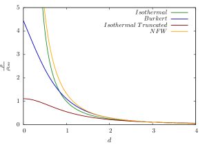
Figure 1: Plots of the density profile $\rho(d)$ of the four halos considered. Notice that our chosen calibration is such that the densities are equal at $d=3$ in the four cases.

Given the density profile $\rho$, we can find that the halo mass distribution $m(r)$ as

$$m(r)=4\pi\int\rho r^{2}dr\;,$$ (52)

so that the gravitational potential is given by $\Phi=-Gm(r)/r$.

Where we can also introduce a dimensionless potential $V(d)$ with the help of the particle mass $m$ and a characteristic speed $\sigma_{0}$ as

$$\Phi(r)=m\,{\sigma_{0}}^{2}V(d)\;,$$ (53)

In this way, the gradient of the gravitational potential can be written as

$$\frac{\partial\Phi(r)}{\partial r}=\frac{m{\sigma_{0}}^{2}}{R_{0}}\;\frac{\partial V(d)}{\partial d}\;.$$ (54)

Making now use of the relation between $\sigma_{0}$ and $\rho_{0}$ given by Eq. (49), the dimensionless gradient of the gravitational potential for each halo becomes:

$$\frac{\partial V_{\rm iso}(d)}{\partial d}=\frac{3}{d}\;, \frac{\partial V_{\rm iso-tr}(d)}{\partial d}=\frac{10\left(1-\frac{\arctan\left(d\right)}{d}\right)}{3d}\;,$$

$$\frac{\partial V_{\rm Burkert}(d)}{\partial d}=\frac{10\left(\ln\left(\left(1+d^{2}\right)\left(1+d\right)^{2}\right)-2\arctan\left(d\right)\right)}{3d^{2}}\;, \frac{\partial V_{\rm NFW}(d)}{\partial d}=\frac{16\left(\ln\left(1+d\right)-\frac{d}{1+d}\right)}{d^{2}}\;.$$

At this point it is also convenient to rewrite the Vlasov equation, Eq. (29), in a dimensionless form. As already mentioned, defining a pattern mass $M_{0}$ and a pattern distance $R_{0}$ allows us to define a pattern density $\rho_{0}$ and from it a pattern velocity $\sigma_{0}$. Considering that we are dealing with a single type of particles characterized by a mass $m$, we can continue this idea and construct all the needed pattern quantities, i.e. a pattern time $T_{0}=R_{0}/\sigma_{0}$, a pattern radial momentum $p_{0}=m\sigma_{0}$, and a pattern angular momentum $l_{0}=m\,\sigma_{0}\,R_{0}$. Rewriting then the time as $t=T_{0}\,{\cal T}$, the radial momentum as $p_{r}=p_{0}\,{\cal P}_{r}$, and the angular momentum as $L=l_{0}\,{\cal L}$, we obtain the following dimensionless Vlasov equation:

$$\frac{\partial\cal{F}}{\partial{\cal T}}=-{\cal P}_{r}\,\frac{\partial\cal{F}}{\partial d}+\left(\frac{\partial V(d)}{\partial d}-\frac{{\cal L}^{2}}{d^{3}}\right)\frac{\partial\cal{F}}{\partial{\cal P}_{r}}\;,$$ (56)

where we have defined $f=f_{0}\,\cal{F}$, with $\cal{F}$ a dimensionless distribution function, and $f_{0}$ a normalization constant with units of probability density in phase space.

For each halo model, we use the dimensionless gradient of the gravitational potential given by Eqs. (LABEL:eqs:phisd), in order to evolve the distribution function. The corresponding dimensionless potentials are given by:

$$V_{\rm iso}(d)=3\ln(d)\;,\hskip 199.16928ptV_{\rm iso-tr}(d)=\frac{5}{3}\left(\ln(1+d^{2})+2\frac{\arctan(d)}{d}\right)\,,$$

(57)

$$V_{\rm Burkert}(d)=\frac{10}{3d}\left(2\left(1+d\right)\left(\arctan\left(d\right)-\ln\left(1+d\right)\right)-\left(1-d\right)\ln\left(1+d^{2}\right)\right)\;,\hskip 28.45274ptV_{\rm NFW}(d)=-16\frac{\ln(1+d)}{d}\;.$$

The dimensionless effective potential is obtained by adding the centrifugal term. Fig (2) shows the plots for the effective potential in each case.

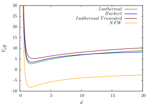
Figure 2: Plots of the effective dimensionless potential of the four halos considered with ${\cal L}=3.5$.

The profiles for the potential gradients are shown in Figure (3), and the corresponding graphs for the gradient of the effective potential (including the centrifugal term) are shown in Figure (4).

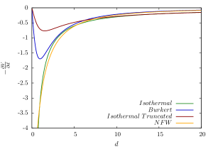
Figure 3: Plots for minus the derivative of the dimensionless gravitational potential $V(d)$ for each of the four halos considered.

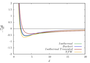
Figure 4: Plots for the derivative of the effective dimensionless gravitational potential for the four halos considered with ${\cal L}=3.5$.

IV Numerical code

In this section, we describe our Vlaso-ollin code, which evolves the distribution function by means of the Vlasov equation, Eq.(56) for several background gravitational potentials.

IV.1 Flux conservative methods

The Vlasov equation (56) can be trivially rewritten in conservation form as:

$$\frac{\partial\cal{F}}{\partial{\cal T}}+\frac{\partial}{\partial d}\left[{\cal P}_{r}{\cal F}\right]+\frac{\partial}{\partial{\cal P}_{r}}\left[\left(\frac{\partial V(d)}{\partial d}-\frac{{\cal L}^{2}}{d^{3}}\right){\cal F}\right]=0\;.$$ (58)

We will now define the fluxes in the $d$ and ${\cal P}_{r}$ directions, $F_{d}$ and $F_{{\cal P}_{r}}$, as

$$F_{d}\equiv{\cal P}_{r}{\cal F}\;,\quad F_{{\cal P}_{r}}\equiv\frac{\partial V_{\rm eff}(d)}{\partial d}{\cal F}\;,$$ (59)

where as before

$$V_{\rm eff}\equiv V(d)+\frac{1}{2}\frac{{\cal L}^{2}}{d^{2}}\;.$$ (60)

The Vlasov equation then becomes

$$\frac{\partial\cal{F}}{\partial\cal{T}}+\frac{\partial F_{d}}{\partial d}+\frac{\partial F_{{\cal P}_{r}}}{\partial{\cal P}_{r}}=0\;.$$ (61)

We have written a numerical code to solve the last equation using a flux conservative finite difference method Leveque92 . A crucial consequence of a using conservative method for the Vlasov equation is that the numerical integration will conserve the total number of particles $N$ exactly (up to machine round-off error), so that any change in the number of particles will be the result of particles leaving (or entering) the computational domain through the boundaries.

In our code phase-space is discretized in a rectangular grid of size $N_{r}\times N_{p}$, with $0\leq d\leq d_{max}$ and $-{\cal P}_{max}\leq{\cal P}\leq{\cal P}_{max}$, and with grid sizes $\Delta d$ and $\Delta{\cal P}$. The code uses a method of lines, with a three-step iterative Crank-Nicholson time integrator. We use a flux-limiter method for the calculation of the fluxes $F_{d}$ and $F_{{\cal P}_{r}}$ at the cell interfaces. The limiter methods minmod, van Leer, superbee and monotonized-centered (MC) Leveque92 were tested for the special case of an external potential corresponding to a constant density star, and particles with zero angular momentum, and the MC limiter was found to show the best results in both preserving the number of particles and preserving the form of the density profile for stationary solutions: minmod is very diffusive in the sense that stationary profiles tend to diminish in amplitude and become wider (while conserving the integral), while the van Leer and superbee limiters, though less diffusive, in general deform the stationary profiles. The reason why we found it necessary to use sophisticated high resolution flux-limiter methods is because such methods can be shown to be total-variation-diminishing (TVD), and this guarantees that the solution has no spurious oscillations. This ensures that in regions where the distribution function $f$ is close to zero it remains well behaved and does not become negative (which would be unphysical, but can easily happen with numerical methods that are not TVD). The limiter methods we use are second order accurate everywhere except at extrema of the distribution function, where they become only first order.

IV.2 Boundary conditions

There are two different types of boundaries to consider in our simulations: the external boundaries of the computational domain at $|{\cal P}|={\cal P}_{max}$ and $d=d_{max}$, and the internal boundary at $d=r=0$.

For the external boundaries the boundary condition we use depends on the sign of the coefficient of the corresponding derivative. That is, in the radial direction we consider the sign of the momentum ${\cal P}_{r}$: For negative values of ${\cal P}_{r}$, corresponding to particles that would enter the computational domain, we just set the distribution function $f$ to zero, while for positive values of ${\cal P}_{r}$, corresponding to particles leaving the domain, we calculate the fluxes all the way to the boundary using one-sided differences. In the momentum directions we do the same thing, but in this case we consider the sign of the force term $\partial V_{\rm eff}(d)/\partial d$.

The boundary at $d=r=0$ is of a different type and corresponds to the origin of the radial coordinate. Notice that at $r=0$ the centrifugal term becomes singular, and the gravitational force can also become singular for some of the halo models we are considering (the isothermal and NFW models). To avoid dealing with singular quantities we use a finite differencing grid that staggers the origin, so that the first grid point is located at $d=\Delta d/2$. We add a fictitious point at $d=-\Delta d/2$ in order to be able to calculate derivatives at $d=0$. This fictitious point also allows us to impose adequate parity conditions on the different quantities.

Now, in the case of non-zero angular momentum the particles are never allowed to reach the origin so that the distribution function $f$ should be zero there. But in the case of zero angular momentum there is nothing to stop them from reaching $r=0$. If moreover, the gravitational potential is regular there (as in the case of the truncated-isothermal and Burkert models), the particles that reach the origin can in principle just come back on the opposite side and oscillate around the origin. This is in fact an interesting case, as particles that reach the origin with a given negative radial momentum will move back out of the origin with a positive radial momentum. In order to capture this behavior we use the fictitious points at $d=-\Delta d/2$ to impose the boundary condition $f(-d,-{\cal P}_{r})=f(d,{\cal P}_{r})$. We find that when doing so, particles with zero angular momentum in a regular potential just describe orbits around the origin of phase space, in a very similar way as one would expect for the case of a simple harmonic oscillator.

When the angular momentum is non-zero, particles coming from infinity should reach a finite minimum radius, so in principle one would not need a special boundary condition at $d=0$. In practice, however, we have found that in this case the distribution function $f$ might still attain small non-zero values at $d=r=0$ due to numerical errors, and using the boundary condition described above results in robust evolutions.

There is a final important point that should be made about the behavior of the distribution function $f$ at the origin for the case of zero angular momentum. From the definition of the particle density $\rho_{f}$ and the momentum density $j_{f}$, equations (8) and (9), one can easily see that if the distribution function $f$ does not vanish at the origin then $\rho_{f}$ and $j_{f}$ will be singular there (in fact, $f$ must vanish at least as $r^{2}$). This actually makes perfect physical sense: if an infalling spherical shell of matter reaches the origin at the same time, then the matter density will clearly become infinite there as all the particles are now at a single point. For an external (regular) gravitational potential this represents no problem since we can just interpret the distribution function statistically: every individual particle behaves independently of the others and will just oscillate around the origin. But if we were to consider the case of self-gravitating particles, then as they reach the origin the mass density will become infinite there, so that the gravitational potential will become singular, and our description in terms of the Vlasov equation will break down. All the simulations shown below will be for the case of an external gravitational potential (the particles have no self-gravity) and non-zero angular momentum, so that this problem will never arise, but it is something that should be kept in mind for the study of systems of self-gravitating particles with the Vlasov equation.

IV.3 CFL condition

Since we are using an explicit scheme, in order to get a stable evolution we need to satisfy the Courant-Friedrichs-Lewy (CFL) condition. During the evolution we then choose the time step as $\Delta t=\min(\Delta t_{d},\Delta t_{p})$, with

$$\Delta t_{d}=\frac{C\Delta d}{{\cal P}_{max}}\;,\qquad\Delta t_{p}=\frac{C\Delta{\cal P}}{|F|_{max}}\;.$$ (62)

where $F\equiv\partial V_{\rm eff}(d)/\partial d$ and $C$ a number of order 1 which in two dimensions must be such that $C\leq 1/\sqrt{2}$. In all the simulations shown below we choose $C=0.7$ and $P_{max}=6$. The maximum value of the force $F_{max}$ is calculated a $t=0$ and does not change in time since the background potential is fixed.

The fact that the centrifugal term ${\cal L}/d^{3}$ in the effective force diverges at $d=0$ is a serious problem and forces us to use very small values for $\Delta t$ in order to satisfy the CFL condition. In order to avoid this problem we introduce a small parameter $\epsilon$ in the denominator that modifies the centrifugal potential for small values of $d$, and the modified centrifugal force is obtained by deriving the new potential.

$$\frac{{\cal L}^{2}}{d^{2}} \longrightarrow \frac{{\cal L}^{2}}{d^{2}+\epsilon^{2}}\;,$$

$$\frac{{\cal L}^{2}}{d^{3}} \longrightarrow \frac{{\cal L}^{2}\,d}{(d^{2}+\epsilon^{2})^{2}}\;.$$ (63)

For a given value of the angular momentum ${\cal L}$ we choose $\epsilon$ in such a way as to guarantee that the centrifugal force is minimally modified at the smallest radius that can be reached by a particle with that angular momentum. Assuming that the particle starts far away with initial momentum ${\cal P}_{i}$, and that for small values of $d$ the centrifugal force dominates over the gravitational force, then conservation of energy implies that the minimum radius the particle can reach is such that ${\cal L}^{2}/d_{\rm min}^{2}\sim{{\cal P}_{i}}^{2}/2m$, which implies $d_{\rm min}\sim\sqrt{2m}\;{\cal L}/|{\cal P}_{i}|$. In our simulations we typically take $\epsilon=d_{min}/10$.

This is clearly not an ideal solution as in involves modifying the effective force so that a small error is introduced for small radii, and in practice still results in values of $\Delta t$ that are much smaller than $\Delta d$, so that our code is rather slow. We are exploring ways to improve our code, perhaps by using an operator splitting method with an implicit scheme for the centrifugal term. We will report on this elsewhere.

IV.4 Initial data

For our simulations we consider an initial localized distribution of particles in phase space, in the background gravitational potential of the different halo models. We interpret this as a inhomogeneity in the dark matter halo, and use the Vlasov equation to determine the final state of such perturbation.

We consider an initial phase space distribution $f$ given as

$$f(t=0)=\frac{N_{0}}{8\pi^{3}L_{0}\sigma_{d}\sigma_{\cal P}}\left(e^{-\frac{(d-d_{0})^{2}}{{\sigma_{d}}^{2}}}e^{-\frac{({\cal P}_{d}-{{\cal P}_{r}}_{0})^{2}}{{\sigma_{\cal P}}^{2}}}+e^{-\frac{(d+d_{0})^{2}}{{\sigma_{d}}^{2}}}e^{-\frac{({\cal P}_{d}+{{\cal P}_{d}}_{0})^{2}}{{\sigma_{\cal P}}^{2}}}\right)\;.$$ (64)

This is normalized so that the total number of particles is $N_{0}$, and in all our simulations we take $N_{0}=1$. Notice that, when the angular momentum is zero, the normalization factor in the initial distribution is instead $1/(4\pi^{2}\sigma_{r}\sigma_{\cal P})$.

The above initial data represents a spherical shell of particles, all of which have the same angular momentum $L_{0}$, with a Gaussian distribution centered at a radius $d_{0}$ and radial momentum ${{\cal P}_{d}}_{0}$, with widths $\sigma_{d}$ and $\sigma_{\cal P}$ respectively. The initial data is constructed so that the symmetry $(d,{\cal P})\to(-d,-{\cal P})$ discussed above when we described the boundary conditions is preserved (incidentally, this form of the initial data also guarantees that the normalization is exact when integrating over the radial coordinate from 0 to infinity). We remind the reader at this point that even if all the particles have the same angular momentum $L_{0}$, by construction their individual motions are uniformly distributed in all angular directions, so that the overall spherical symmetry is preserved. For the simulations shown below we take the following parameters for the initial data: $d_{0}=3.0$, ${{\cal P}_{d}}_{0}=-0.5$, $\sigma_{d}=0.5$, and $\sigma_{\cal P}=0.25$. The corresponding initial data is shown in Figure (5).

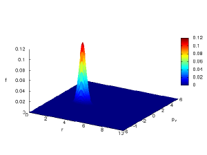
Figure 5: Initial distribution function in phase space for $N_{0}=1$, $d_{0}=3.0$, ${{\cal P}_{d}}_{0}=-0.5$, $\sigma_{d}=0.5$, and $\sigma_{\cal P}=0.25$.

V Results

The time evolution of the initial distribution function $\mathcal{F}$ is given by solving equation (58) in the numerical mesh. We perform a series of simulations for different values of the angular momentum, $L=2.0,2.5,3.0,3.5$. We have not considered smaller values of the angular momentum because in those cases we have found that the particles fall very rapidly to the center, while larger vales of the angular momentum result in the particles escaping the computational domain. In all our evolutions we also fix the mass of the individual particles to $m=1$.

For the simulations shown below we considered two different resolutions $\Delta d=\Delta{\cal P}=0.05$ and $\Delta d=\Delta{\cal P}=0.1$. The boundaries of the computational domain are located at $d_{max}=20$ and ${\cal P}_{max}=6$. This range is chosen so that at the higher resolution we use only a very small fraction of the particles has escaped through the boundaries at the end of the simulation. As we will see below, that particles that escape do so mostly because of numerical dissipation.

V.1 Time evolution for $\mathcal{L}=3.5$

As an example of the dynamics of the Vlasov equation, in this section we will concentrate on presenting the results of the time evolution of the distribution function for the case of our largest value of the angular momentum, namely $\mathcal{L}=3.5$.

Figures 6-9 show the evolution of the distribution function for our four different halo models. In each figure we show six snapshots at different times during the evolution. The first five snapshots correspond to the same times in all cases, namely $\mathcal{T}=0,9.33,18.84,30.79,45.71$. The time corresponding to the last snapshot differs for each halo model because in each case we show an epoch when the system has finally reached a stationary state. Figure 10 shows again the final stationary distribution function in phase space for the four different models. We can see that all four halo models the distribution function reaches a stationary state that corresponds to orbits in phase space around a central point. This is not surprising, since individual particles with a given angular momentum are expected to have orbits around the center of gravity with some minimum and maximum radii (the individual orbits will not be precisely elliptical since the potentials for the different halos are not simply $1/d$). The stationary states look similar for each halo model, even if they are not reached at the same time; for the isothermal, Burkert and NFW models the stationary state is reached at time $\mathcal{T}\sim 120$ and for the truncated isothermal this state is reached at time $\mathcal{T}\sim 260$. Next, in Figures 11-14 we show the time evolution of the integrated particle density $\rho_{f}(d)$ for the four halo models and the same times as before. Again we see how even though the initial stages of the evolution are different for each halo model, the final stationary particle density is quite similar, with a characteristic two-hump shape corresponding to particles that describe an orbit in phase space and accumulate mostly at the extrema of those orbits as seen in physical space.

Even though we have only shown the case with angular momentum $\mathcal{L}=3.5$, simulations with different values of the angular momentum behave in a very similar way.

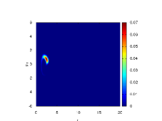
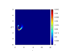
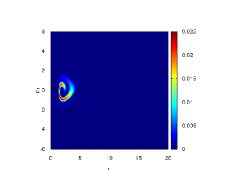
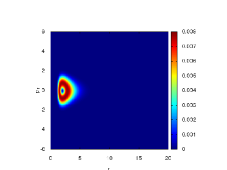
Figure 6: Time evolution of the distribution function $\mathcal{F}$ for the isothermal model with angular momentum $\mathcal{L}=3.5$. The different panels correspond to times $\mathcal{T}=0,9.33,18.84,30.79,45.71,200.39$.

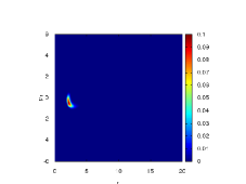
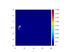
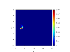
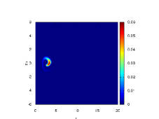
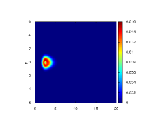
Figure 7: Time evolution of the distribution function $\mathcal{F}$ for the truncated isothermal model with angular momentum $\mathcal{L}=3.5$. The different panels correspond to times $\mathcal{T}=0,9.33,18.84,30.79,45.71,259.38$.

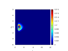
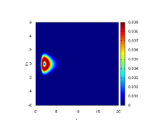
Figure 8: Time evolution of the distribution function $\mathcal{F}$ for the Burkert model with angular momentum $\mathcal{L}=3.5$. The different panels correspond to times $\mathcal{T}=0,9.33,18.84,30.79,45.71,196.85$.

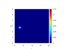
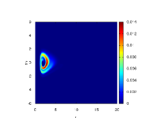
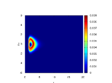
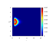
Figure 9: Time evolution of the distribution function $\mathcal{F}$ for the NFW model with angular momentum $\mathcal{L}=3.5$. The different panels correspond to times $\mathcal{T}=0,9.33,18.84,30.79,45.71,189.20$.

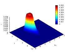
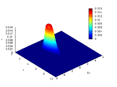
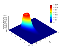
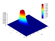
Figure 10: Final virialized distribution function for the four different halo models with angular momentum $\mathcal{L}=3.5$. Starting in the top left panel: isothermal, truncated isothermal, Burkert and NFW.

Figure 11: Time evolution of the integrated particle density $\rho_{f}(d)$ multiplied for the $d^{2}$ factor for the isothermal model with angular momentum $\mathcal{L}=3.5$. The different panels correspond to times $\mathcal{T}=0,9.33,18.84,30.79,45.71,200.39$, same that those in Figure 6.

Figure 12: Time evolution of the integrated particle density $\rho_{f}(d)$ multiplied for the $d^{2}$ factor for the isothermal truncated model with angular momentum $\mathcal{L}=3.5$. The different panels correspond to times $\mathcal{T}=0,9.33,18.84,30.79,45.71,259.38$, same that those in Figure 7.

Figure 13: Time evolution of the integrated particle density $\rho_{f}(d)$ multiplied for the $d^{2}$ factor for the Burkert model with angular momentum $\mathcal{L}=3.5$. The different panels correspond to times $\mathcal{T}=0,9.33,18.84,30.79,45.71,196.85$, same that those in Figure 8.

Figure 14: Time evolution of the integrated particle density $\rho_{f}(d)$ multiplied for the $d^{2}$ factor for the NFW model with angular momentum $\mathcal{L}=3.5$. The different panels correspond to times $\mathcal{T}=0,9.33,18.84,30.79,45.71,189.20$, same that those in Figure 9.

V.2 One particle motion

In order to understand the results from the previous section, it is perhaps instructive to consider the motion of a single particle in a gravitational potential determined by the different halo models considered.

For a particle starting at an initial radius $d_{0}$, with initial radial momentum ${{\cal P}_{d}}_{0}$, and with a given angular momentum $L$, conservation of energy implies that

$$\frac{{{\cal P}_{d}}^{2}}{2m}+\frac{{\cal L}^{2}}{2md^{2}}+\Phi(d)=\frac{{{{\cal P}_{d}}_{0}}^{2}}{2m}+\frac{{\cal L}^{2}}{2m{d_{0}}^{2}}+\Phi(d_{0})\;.$$ (65)

From this one can determine the turning points of the orbit, or the radius of a circular orbit for a given value of the angular momentum.

$\cal L$	$V$	Turning points		$\rho_{max}$
		$d_{min}$	$d_{max}$	$d$
2	Isothermal	1.03	3.18	0.8
2	Iso. Trun.	1.59	3.33	1.25
2	Burkert	1.16	3.19	0.92
2	NFW	0.95	3.15	0.75
2.5	Isothermal	1.44	3.23	1.02
2.5	Iso. Trun.	2.06	3.49	1.67
2.5	Burkert	1.56	3.25	1.17
2.5	NFW	1.31	3.19	0.97
3	Isothermal	1.88	3.33	1.32
3	Iso. Trun.	2.46	3.85	2.02
3	Burkert	2.00	3.37	1.47
3	NFW	1.72	3.26	1.23
3.5	Isothermal	2.35	3.58	1.65
3.5	Iso. Trun.	2.69	4.54	2.32
3.5	Burkert	2.41	3.67	1.77
3.5	NFW	2.17	3.41	1.52

Table 1: Positions of the turning points for each configuration of angular moment and halo potential and position of the maximum density value at the final virialized distribution function.

It is interesting to note that the turning points for a single particle with initial position and momentum corresponding to the maximum of the initial phase space distribution does not coincide with the position of the maxima of the integrated energy density in the equilibrium state (Table 1). The reason for this, may be the so-called statistical pressure: even though the particles are non interacting, it seems that the collective motion is different from the individual motion of particles initially at the center of the distribution.

V.3 Virialization

As mentioned above, in all our simulations the evolution of the distribution function eventually reaches a stationary state. Such a state should satisfy the virial theorem, equation (41). In order to verify this we compute the average of the radial kinetic energy $\left<{{\cal P}_{d}}^{2}/2m\right>$, and the average of the virial $\left<F_{\rm eff}(d)\,d\right>$, and compare them during the evolution.

We find that in each case, as the initial distribution evolves toward a stationary state, the average of the radial kinetic energy and the average of the virial both reach constant values that satisfy the virial theorem (41). Figures 15-18 show plots of $\left<{{\cal P}_{d}}^{2}/2m\right>$ and $\left<-F_{\rm eff}(d)\,d/2\right>$ for each of the different halo models, and for four values of the angular momentum in each case. We find that in each case, after strong initial oscillations, the average kinetic energy and virial reach a constant value satisfying the virial theorem. We also find that this virialization process takes longer for larger values of the angular momentum, while that the final constant value of the average kinetic energy becomes smaller. Notice also that while $\left<{{\cal P}_{r}}^{2}/2m\right>$ is always positive, $\left<-F_{\rm eff}(d)\,d/2\right>$ can become negative during the initial portions of the evolution.

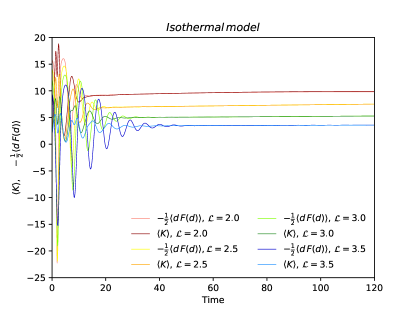
Figure 15: Virialization for the case of the isothermal model for different values of the angular momentum $\mathcal{L}=2.0,2.5,3.0,3.5$.

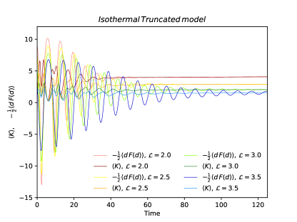
Figure 16: Virialization for the case of the truncated isothermal model for different values of the angular momentum $\mathcal{L}=2.0,2.5,3.0,3.5$.

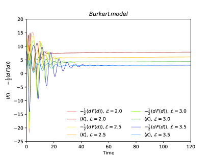
Figure 17: Virialization for the case of the Burkert model for different values of the angular momentum $\mathcal{L}=2.0,2.5,3.0,3.5$.

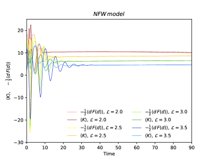
Figure 18: Virialization for the case of the NFW model for different values of the angular momentum $\mathcal{L}=2.0,2.5,3.0,3.5$.

Figure 19 shows a comparison of the virialization process for the four different halo models in the specific case with angular momentum ${\cal L}=3.5$. We can see that the NFW model virializes very rapidly, while the truncated isothermal model takes much longer than all other models to virialize. Again we see that models that take longer to virialize reach smaller values of the final average kinetic energy.

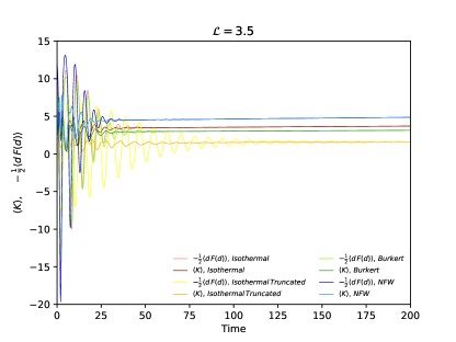
Figure 19: Comparison of the virialization process for the different halo models in the case with $\mathcal{L}=3.5$.

V.4 Conservation of particles

As mentioned above, since we are using a conservative numerical method, the total number of particles defined in (11) should be conserved up to machine round off error in our simulations. Changes in the total number of particles should reflect only the particles that leave the computational domain through the external boundaries. We find, however, that numerical diffusion can cause particles to reach the boundaries that would not do so physically.

In order to illustrate this behavior, in Figures 20 and 21 we show the time evolution of the total number of particles integrated over the whole computational domain, for the different halo models and different values of the angular momentum (we remind the reader that this number has been normalized to $1$ in the initial data). Figure 20 shows the results for low resolution runs with $\Delta d=\Delta{\cal P}=0.1$, while Figure 21 shows the results for the higher resolution runs with $\Delta d=\Delta{\cal P}=0.05$.

There are several things to notice from the figures. First, at large times we are indeed loosing particles through the boundaries. A more detailed analysis of the fluxes through the different boundaries shows that we are loosing them mostly through the boundary at negative momenta. Second, even though at the lower resolution the loss of particles is very significant by the end of the simulations (in one case we loose as much as $70\%$ of the particles), at the higher resolution this loss is much lower (in the worst case only about $8\%$), which indicates that this loss of particles is mostly due to numerical diffusion which becomes smaller at higher resolutions.

Considering only the results from the higher resolution, Figure 21, we notice that more particles are lost for low values of the angular momentum (for ${\cal L}=2.0$ the NWF halo looses $8\%$ of the particles), while for larger angular momentum the loss of particles becomes extremely small (for ${\cal L}=3.5$ the NFW halo looses only about $0.0007\%$). We also notice that the NFW halo is the one which has more trouble keeping the particles inside the computational domain whereas the truncated isothermal is the one which best preserves the total number of particles.

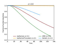
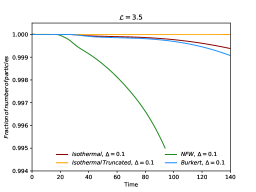
Figure 20: Total number of particles integrated over the complete computational domain for the different halo models, and different values of the angular momentum ${\cal L}$, for a resolution of $\Delta d=\Delta{\cal P}=0.1$.

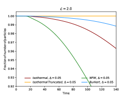
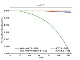
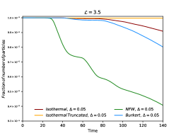
Figure 21: Total number of particles integrated over the complete computational domain for the different halo models, and different values of the angular momentum ${\cal L}$, for a resolution of $\Delta d=\Delta{\cal P}=0.05$.

VI Discussion

We have studied the (Newtonian) Vlasov equation in spherical symmetry for the case of particles moving in a background gravitational potential. We have shown that in this case the problem effectively reduces to that of a three-dimensional phase-space corresponding to the radial coordinate $r$, the radial momentum $p_{r}$, and the total angular momentum $L$. Moreover, since the angular momentum is conserved, it can effectively be decoupled from the other phase space coordinates, so that one can consider the motion of particles all of which have the same value of the angular momentum $L_{0}$, reducing the problem to a two-dimensional case. We have constructed a numerical code to solve directly the Vlasov equation given several values of angular momenta $L_{0}$ using a conservative TVD (flux limiter) scheme.

We have used our code to study the evolution of an initial localized distribution of particles in phase space in the background gravitational potential of four different models for a dark matter halos, namely the isothermal, truncated isothermal, Burkert and NFW models. We interpret this initial distribution as a inhomogeneity in the dark matter halo. Knowing that the resulting Vlasov equation implies the continuity equation and also the standard virial theorem for stationary solutions, we have used these results for testing the corresponding temporal evolution. We find that, for all the cases considered, during evolution the initial distribution leads to non-trivial stationary final distributions that satisfy the virial theorem. The detailed properties of such final distributions change from one type of halo to another, but the overall features are very similar. We believe the detailed study of the evolution of such inhomogeneities could be relevant to characterize the observed halos.

Even though the virial theorem has to be satisfied for equilibrium states, by itself it does not tell us under what conditions an arbitrary initial configuration will evolve toward a stationary configuration, nor how such an evolution will develop. It is well known that an arbitrary distribution that depends only on conserved quantities like the total energy $E$ and angular momentum $L$, $f=f(E,L)$, is automatically a stationary solution of the Vlasov equation. However, for arbitrary initial configurations such as those studied here, we can’t predict a priori what stationary solution will be reached, or even if such a stationary situation will be reached. As we have seen, the increase of entropy is not a useful concept in this case, since the Vlasov equation preserves entropy. We therefore believe that the use of ergodic theory might be useful in this case.

It is important to mention that the dynamical description of dark matter when seen from the point of view of kinetic theory, as has been done here, differs from the standard description in terms of N-body simulations Harker:2005um , though of course both descriptions should coincide in the limit of a very large number of bodies Colombi:2015eia

Still, a statistical description in terms of kinetic theory allows us to define a continuous distribution of matter, as opposed to a discrete number of point particles, which could have important advantages and in particular would be easier to generalize to the case of general relativity (where point particles are conceptually problematic). Also, our description here is very different from other approaches that consider dark matter as a type of fluid as in Barranco:2013wy , or as a ultra-light scalar field as in Burt:2011pv ; Barranco:2012qs ; Barranco:2013rua .

The results obtained and presented in this manuscript are encouraging, showing that dark matter inhomogeneities can be well described by kinetic theory, leading to non-trivial equilibrium configurations. With these results, there are two clear avenues for further research. The first is to consider the case of particles with a distribution of different values of the angular momentum, which would require a three-dimensional code for the phase space coordinates ($r,p_{r},L$). On the other hand, one can consider the case of a system of self-gravitating particles, which would require us to solve the Poisson equation to obtain the gravitational potential. And of course, one can move away from the simple Newtonian description to a general relativistic one (see e.g. MartinGarcia:2001nh ; Akbarian:2014gna ). All these problems are currently being investigated, and we will report their progress in the near future.

References

- (1) Teresa Marrodán Undagoitia and Ludwig Rauch. Dark matter direct-detection experiments. J. Phys., G43(1):013001, 2016.
- (2) D. S. Akerib et al. The Large Underground Xenon (LUX) Experiment. Nucl. Instrum. Meth., A704:111–126, 2013.
- (3) R. Bernabei et al. The DAMA/LIBRA apparatus. Nucl. Instrum. Meth., A592:297–315, 2008.
- (4) D. Yu. Akimov et al. The ZEPLIN-III dark matter detector: instrument design, manufacture and commissioning. Astropart. Phys., 27:46–60, 2007.
- (5) E. Aprile, J. Angle, F. Arneodo, L. Baudis, A. Bernstein, A. Bolozdynya, P. Brusov, L. C. C. Coelho, C. E. Dahl, L. DeViveiros, A. D. Ferella, L. M. P. Fernandes, S. Fiorucci, R. J. Gaitskell, K. L. Giboni, R. Gomez, R. Hasty, L. Kastens, J. Kwong, J. A. M. Lopes, N. Madden, A. Manalaysay, A. Manzur, D. N. McKinsey, M. E. Monzani, K. Ni, U. Oberlack, J. Orboeck, D. Orlandi, G. Plante, R. Santorelli, J. M. F. dos Santos, P. Shagin, T. Shutt, P. Sorensen, S. Schulte, E. Tatananni, C. Winant, and M. Yamashita. Design and performance of the XENON10 dark matter experiment. Astroparticle Physics, 34:679–698, April 2011.
- (6) J. Barreto et al. Direct Search for Low Mass Dark Matter Particles with CCDs. Phys. Lett., B711:264–269, 2012.
- (7) Alvaro E. Chavarria et al. DAMIC at SNOLAB. Phys. Procedia, 61:21–33, 2015.
- (8) A. Aguilar-Arevalo et al. First direct detection constraints on eV-scale hidden-photon dark matter with DAMIC at SNOLAB. Submitted to: Phys. Rev. Lett., 2016.
- (9) A. Aguilar-Arevalo et al. Search for low-mass WIMPs in a 0.6 kg day exposure of the DAMIC experiment at SNOLAB. Phys. Rev., D94(8):082006, 2016.
- (10) Juan Barranco, Argelia Bernal, and Darío Núñez. Dark matter equation of state from rotational curves of galaxies. Mon. Not. Roy. Astron. Soc., 449(1):403–413, 2015.
- (11) Tonatiuh Matos, Francisco Siddhartha Guzman, and L. Arturo Urena-Lopez. Scalar field as dark matter in the universe. Class. Quant. Grav., 17:1707–1712, 2000.
- (12) Tonatiuh Matos and L. Arturo Urena-Lopez. Scalar field dark matter, cross section and Planck-scale physics. Phys. Lett., B538:246–250, 2002.
- (13) Tonatiuh Matos, Argelia Bernal, and Dario Nunez. Flat Central Density Profiles from Scalar Field Dark Matter Halo. Rev.Mex.A.A., 44:149, 2008.
- (14) Julio F. Navarro, Carlos S. Frenk, and Simon D. M. White. The Structure of cold dark matter halos. Astrophys. J., 462:563–575, 1996.
- (15) Geraint Harker, Shaun Cole, John Helly, Carlos Frenk, and Adrian Jenkins. A marked correlation function analysis of halo formation times in the millennium simulation. Mon. Not. Roy. Astron. Soc., 367:1039–1049, 2006.
- (16) E. Athanassoula, E. Fady, J. C. Lambert, and A. Bosma. Optimal softening for force calculations in collisionless n-body simulations. Monthly Notices of the Royal Astronomical Society, 314(3):475, 2000.
- (17) Walter Dehnen. Towards optimal softening in three-dimensional n-body codes — i. minimizing the force error. Monthly Notices of the Royal Astronomical Society, 324(2):273, 2001.
- (18) R. W. Hockney and J. W. Eastwood. Computer Simulation Using Particles. 1981.
- (19) Jasjeet Singh Bagla. Cosmological N-body simulation: Techniques, scope and status. Curr. Sci., 88:1088, 2005.
- (20) J. Binney and S. Tremaine. Galactic Dynamics. Princeton Series in Astrophysics. Princeton University Press, second edition, 2008.
- (21) S. Colombi, T. Sousbie, S. Peirani, G. Plum, and Y. Suto. Vlasov versus N-body: the Henon sphere. Mon. Not. Roy. Astron. Soc., 450(4):3724–3741, 2015.
- (22) Hakan Andreasson. The Einstein-Vlasov system / kinetic theory. Living Rev. Rel., 8:2, 2005.
- (23) S. L. Shapiro and S. A. Teukolsky. Black holes, white dwarfs, and neutron stars: The physics of compact objects. Wiley, 1983.
- (24) Paola Domínguez-Fernández. On particle dynamics: Vlasov equation and dark matter, UNAM-Mex. Bachelor thesis, UNAM-Mex, 2015.
- (25) Erik Jiménez-Vázquez. Numerical simmulation of the Vlasov-Poisson system in spherical symmetry, UNAM-Mex. Bachelor thesis, UNAM-Mex, 2016.
- (26) R. J. Leveque. Numerical Methods for Conservation Laws. Birkhauser Verlag, Basel, 1992.
- (27) Juan Barranco, Argelia Bernal, Juan Carlos Degollado, Alberto Diez-Tejedor, Miguel Megevand, et al. Are black holes a serious threat to scalar field dark matter models? Phys.Rev., D84:083008, 2011.
- (28) Juan Barranco, Argelia Bernal, Juan Carlos Degollado, Alberto Diez-Tejedor, Miguel Megevand, et al. Schwarzschild black holes can wear scalar wigs. Phys.Rev.Lett., 109:081102, 2012.
- (29) Juan Barranco, Argelia Bernal, Juan Carlos Degollado, Alberto Diez-Tejedor, Miguel Megevand, et al. Schwarzschild scalar wigs: spectral analysis and late time behavior. Phys.Rev., D89(8):083006, 2014.
- (30) Jose M. Martin-Garcia and Carsten Gundlach. Selfsimilar spherically symmetric solutions of the massless Einstein-Vlasov system. Phys. Rev., D65:084026, 2002.
- (31) Arman Akbarian and Matthew W. Choptuik. Critical collapse in the spherically-symmetric Einstein-Vlasov model. Phys. Rev., D90(10):104023, 2014.