Nanoscale Seebeck effect at hot metal nanostructures

Abstract

We theoretically study the electrolyte Seebeck effect in the vicinity of a heated metal nanostructure, such as the cap of an active Janus colloid in an electrolyte, or gold- coated interfaces in optofluidic devices. The thermocharge accumulated at the surface varies with the local temperature, thus modulating the diffuse part of the electric double layer. On a conducting surface with non-uniform temperature, the isopotential condition imposes a significant polarization charge within the metal. Surprisingly, this does not affect the slip velocity, which takes the same value on insulating and conducting surfaces. Our results for specific-ion effects agree qualitatively with recent observations for Janus colloids in different electrolyte solutions. Comparing the thermal, hydrodynamic, and ion diffusion time scales, we expect a rich transient behavior at the onset of thermally powered swimming, extending to microseconds after switching on the heating.

I Introduction

Laser-illuminated metal nanostructures provide versatile local heat engines Baf13 , with optofluidic applications such as trapping of nanoobjects Bra13 ; Lin17 , manipulation of biological cells Lin17b , microflows in capillaries Bre16 , and colloidal assembly Lin17a . Similarly, thermally powered artificial microswimmers rely on the conversion of absorbed heat to motion; experimental realisations include metal-capped Janus particles that are driven by surface forces Jia10 ; But12 ; Bar13 ; Sim16 , and interface floaters that are advected by their self-generated Marangoni flow Gir16 ; Wue14 . Force-free localization and steering have been achieved by temporal Bre14  or spatial Loz16 modulation of the laser power.

These experiments also revealed strong dependencies on material properties: Thus a reversal of the swimming direction was observed upon rendering the particle’s active cap hydrophilic instead of hydrophobic But12 , or upon adding a non-ionic surfactant to the solvent Jia10 . Similarly, copolymer coating of a glass surface increased the thermo-osmotic velocity by one order of magnitude Bre16 .

Most of the cited experiments give evidence for creep flow induced by a temperature gradient in the electric double layer at the active surface. Very recently, a specific-ion effect was reported for silica colloids carrying a gold cap: their swimming velocity in a 10 mM NaCl solution changed significantly when replacing the cation with Lithium, or the anion with hydroxide Sim16 . These findings indicate that self-propulsion depends on the electrolyte Seebeck field Wue10 , confirming previous observations on passive particles in an external temperature gradient, which migrated to the cold in an NaCl solution and to the hot in NaOH Put05 ; Vig10 ; Esl14 . Recently an enhanced Seebeck-induced flow was predicted in confined geometries Die16 .

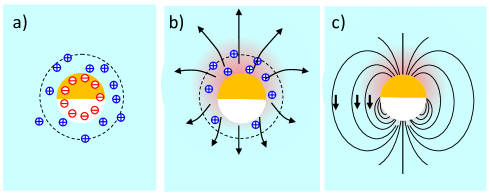
Figure 1: Janus particle with a gold-coated upper hemisphere. a) The electric double layer of a micron-size particle; the diffuse layer of thickness $\lambda\sim$ a few nm, contains a charge $Q\sim 10^{5}e$. b) Upon heating the gold cap, the electrolyte Seebeck effect induces a thermocharge density $\rho_{T}$ which adds to the diffuse layer. We show the case $\rho_{T}>0$; for an excess temperature of a few Kelvin, the total thermocharge is $Q_{T}\sim 100e$ Maj12 . The corresponding negative ions are at the boundary of the experimental cell. The arrows indicate the thermoelectric field. c) Schematic view of the thermoelectric field after subtraction of the monopole term $\propto Q_{T}/r^{2}$. The diffuse layer is not shown. The parallel component $E_{\parallel}$ vanishes at the conducting gold surface; at larger distance one has the dipolar field $\propto r^{-3}$.

In this paper we study how the electrolyte Seebeck effect modifies the electric double layer and drives a creep flow along a surface with non-uniform temperature. The main features are illustrated in Fig. 1 at the example of a gold-capped Janus particle, but are generally valid for metal nanostructures in contact with water Bra13 ; Lin17 ; Lin17b ; Bre16 ; Lin17a . Upon heating the gold cap with a laser, the salt ions move along the temperature gradient, and an excess charge $Q_{T}$ forms at the hot surface, as shown in the middle panel; the corresponding negative ions are at the wall of the container. The resulting electric field comprises, besides the radial monopole term $\propto Q_{T}/r^{2}$, a parallel component along the particle surface; the latter exerts a force on the double layer and induces creep flow.

We address two main questions: First, how are the double layer and the Seebeck field modified by the electrostatic boundary conditions at insulating and conducting surfaces? Second, the equipotential condition at a conductor requires a zero parallel electric field, as illustrated for the upper hemisphere in Fig. 1c. Does this imply that the thermoelectric creep velocity is suppressed at the gold cap of Janus particles?

The outline of our paper is as follows. In Sect. II we briefly review the bulk electrolyte Seebeck effect, where boundary effects are irrelevant. In Sect. III we evaluate the thermocharge and the Seebeck near-field at a surface, which are sketched in Fig. 1 b and c. Starting from the integral expression of Gauss’ law, the thermoelectric properties and the modification of the double-layer are derived both for insulating and conducting surfaces. Sect. V is devoted to the thermodynamic forces resulting from the non-equilibrium state of the double layer, and to the creep flow along the surface. Novel results arise from the parallel component of the thermoelectric and polarization fields derived in Sect. IV. In the final sections we discuss and summarize our results.

II Electrolyte solution in a temperature gradient

We briefly review the steady-state response of an electrolyte solution to a non-uniform temperature Gro62 , the resulting Soret and Seebeck effects, and in particular the thermoelectric field.

II.1 Thermodynamic forces

Consider monovalent ions with concentrations $n_{\pm}$, enthalpy $H_{\pm}$, and chemical potential $\mu_{\pm}=H_{\pm}+k_{B}T\ln n_{\pm}$. Then the ions are subject to the thermodynamic forces, which derive from the Planck potential $\mu_{\pm}/T$ Gro62 ,

$$-T\mathbf{\nabla}\frac{\mu_{\pm}}{T}=-k_{B}T\frac{\mathbf{\nabla}n_{\pm}}{n_{\pm}}+H_{\pm}\frac{\mathbf{\nabla}T}{T},$$ (1)

where the first term in (1) accounts for gradient diffusion, and the second one for thermodiffusion along the temperature gradient. The prefactor of the latter arises from the Gibbs-Helmholtz equation $d(\mu_{\pm}/T)/dT=-H_{\pm}/T^{2}$. Note that this relation does not imply constant enthalpies; the quantities $H_{\pm}$ may depend on temperature.

These thermodynamic forces give rise to ion currents $\mathbf{J}_{\pm}$. When including an electric field $\mathbf{E}$ we find

$$\mathbf{J}_{\pm}=m_{\pm}\left(-k_{B}T\nabla n_{\pm}+n_{\pm}H_{\pm}\frac{\mathbf{\nabla}T}{T}\pm en_{\pm}\mathbf{E}\right),$$ (2)

where we have assumed that the mobilities $m_{\pm}$ are the same for thermodynamic and electric forces, and are related to the diffusion coefficients by $m_{\pm}=D_{\pm}/k_{B}T$. The steady state is, in general, characterized by the condition of constant currents with zero divergency, $\rm{\nabla}\cdot\mathbf{J}_{\pm}=0$. In the case of a closed system with solid boundaries, and in the absence of external forces acting on the ions, however, there is no source field and the currents vanish. In this preliminary section, we consider non-interacting boundaries, and thus put $\mathbf{J}_{\pm}=0$.

II.2 Salt Soret effect

It turns out convenient to consider the salinity $n=(n_{+}+n_{-})/2$ and the charge density $\rho=e(n_{+}-n_{-})$ rather than the ion concentrations $n_{\pm}$. Then the sum of $\mathbf{J}_{\pm}=0$ provides the “Soret equilibrium” for the salinity,

$$\nabla n+nS_{T}\mathbf{\nabla}T=0,$$ (3)

with the salt Soret coefficient

$$S_{T}=\frac{H_{+}+H_{-}}{2k_{B}T^{2}}.$$ (4)

Eq. (3) implies a salinity gradient throughout the sample. Since the enthalpies $H_{\pm}$ are of the order of $k_{B}T$, the relative salinity change is comparable to the relative excess temperature, $\Delta n/n\sim\Delta T/T$. Soret data for various salts were first reported by Chipman in 1926 Chi26 .

II.3 Electrolyte Seebeck effect and surface charges

Now we consider the difference of the equations $\mathbf{J}_{\pm}=0$, which result in a relation for the stationary charge density and electric field. Far from the boundaries, the charge density $\rho$ must vanish because of the huge cost in electrostatic energy required by charge separation. Then we find that, in order to satisfy the zero-current condition, the temperature gradient is accompanied by a constant bulk electric field,

$$\mathbf{E}_{T}=S\mathbf{\nabla}T,$$ (5)

with the coefficient

$$S=-\frac{H_{+}-H_{-}}{2eT}.$$ (6)

$\mathbf{E}_{T}$ is called the macroscopic thermoelectric field, in analogy to the Seebeck effect in metals and semiconductors Put05 . In the latter, the Seebeck coefficient is determined by the temperature dependence of electronic properties, whereas for an electrolyte solution, $S$ is given by the difference of ion enthalpies. Depending on the $H_{\pm}$, the Seebeck coefficient may take either sign; typical values are of the order of $10^{-4}\,\mathrm{V/K}$ Wue10 . In the literature one often finds the “heat of transport” $Q_{\pm}=-H_{\pm}$ with the opposite sign; the most complete data so far are reported in Ref. Nak88 . The above derivation of the Seebeck field has first been given by Guthrie Gut49 , relying on the conditions of zero ion currents and zero charge.

Like any static electric field, $\mathbf{E}_{T}$ must originate from positive and negative charges. Starting from $\mathbf{J}_{\pm}=0$ and allowing for finite $\rho$, we obtain a relation for the stationary charge density and electric field,

$$\nabla\rho+\frac{\varepsilon}{\lambda^{2}}(S\mathbf{\nabla}T-\mathbf{E})=0,$$ (7)

with the Debye length $\lambda^{2}=\varepsilon k_{B}T/2ne^{2}$. Adding Gauss’ law

$$\mathbf{\nabla}\cdot\varepsilon\mathbf{E}=\rho$$ (8)

one finds that the only solution in the bulk corresponds to (5) with $\rho=0$. At the hot and cold boundaries, however, there are finite thermocharge densities $\rho_{T}$ of opposite sign. In physical terms, the thermocharges originate from the unlike thermodiffusion of the cations and anions in (2).

We briefly summarize the above derivation of the electrolyte Seebeck effect. It arises from the tendency of salt ions to migrate along a temperature gradient. The underlying thermodynamic forces $H_{\pm}\nabla T/T$ follow from the entropy balance of the non-equilibrium electrolyte solution Gro62 . Regarding the salt concentration $n=\frac{1}{2}(n_{+}+n_{-})$, the Soret equilibrium (3) describes the stationary salinity gradient; in physical terms it satisfies the steady-state condition, requesting that diffusion and thermodiffusion currents of salt cancel each other.

The Seebeck effect presents a more intricate situation, since it stems from the difference of cation and anion currents. An enthalpy difference $H_{+}\neq H_{-}$, tends to partly separate positive and negative ions. As an important consequence, this results in surface charges and a macroscopic thermoelectric field. Thus one has to satisfy Gauss’ law, in addition to the steady-state condition.

For a negative Seebeck coefficient, the thermodiffusion currents result in positive and negative charges at the hot and cold boundaries, respectively. In the case of a heated particle in a bulk electrolyte solution, the hot boundary reduces to the particle surface, which accordingly is covered by a diffuse layer of mobile cations, as illustrated in Fig. 1b. Then the particle carries a net thermocharge which is related by Gauss’ law to a monopole field that decays as $r^{-2}$ with the distance $r$ Maj12 ; the field lines end at the corresponding anions which are at the wall of the experimental cell. In the present paper we are concerned with the dipolar contribution of the Seebeck field, which is sketched in Fig. 1c.

The linear equations (7) and (8) correspond to the Debye-Hückel approximation. Their solution is generally valid at otherwise uncharged boundaries. Simple 1D and radially symmetric 3D geometries have been studied previously in Maj11 ; Maj12 . The general case of an uncharged surface is treated in Sect. III.2 and in Appendix A. A more complex situation occurs at charged surfaces, since the diffuse layer comprises the counterions and the thermocharge; in the following section this is treated in non-linear Poisson-Boltzmann theory.

III Thermocharge and thermoelectric near-field

Here we evaluate how the thermoelectric properties at the particle surface depend on the material properties, and in particular on its surface charge and electrical conductivity. We first write the usual boundary layer approximation in a form that is well adapted to the condition imposed by the Seebeck far-field.

Thus we calculate the thermocharge density $\rho_{T}$ and the thermoelectric field in the vicinity of the surface. In order to clearly separate the charge effects induced by the temperature gradient from those of the electric double layer, we first study an insulating particle that does not carry surface charges. The strong permittivity contrast between water and typical materials such as polystyrene or silica, simplifies the electrostatic boundary conditions.

Then we consider charged surfaces and, moreover, distinguish insulating and conducting materials. The main difficulty arises from the fact that the diffuse layer contains both the counterions of Fig. 1a and the thermocharge of Fig. 1b, which have to be treated on an equal footing in terms of Poisson-Boltzmann theory.

III.1 Boundary layer approximation

Surface charges of colloidal particles are screened by a diffuse layer of counterions. An analytic mean-field solution exists in one dimension only. It provides a controlled approximation at curved surfaces, as long as the local curvature radius is much larger than the Debye screening length $\lambda$. Then there is a separation of length scales: The properties of the electric double layer vary much more rapidly in perpendicular direction than parallel to the surface.

The resulting approximation is best discussed in terms of Gauss’ law (8). The normal field component varies on the scale of $\lambda$, whereas the permittivity and the parallel electric field vary on the scale of the particle radius $a$. Thus to linear order in $\lambda/a$, Gauss’ law simplifies to

$$\frac{dE_{\perp}}{dz}=\frac{\rho}{\varepsilon},$$ (9)

where $z$ is the distance from the surface. Here and in the following, $E_{\perp}$ points away from the surface; thus for a spherical particle, $E_{\perp}$ is the radial component, and $z=r-a$.

For further use, we integrate from the surface to a distance $B$ that is much larger than the screening length but much smaller than the particle radius, $\lambda\ll B\ll a$, and find

$${E}_{\perp}(B)-{E}_{\perp}(0)=\frac{1}{\varepsilon}\int_{0}^{B}dz\rho(z)\equiv\frac{\sigma}{\varepsilon}.$$ (10)

The second identity defines the charge density per unit area of the diffuse layer. This parameter also determines the double-layer potential $\varphi_{\sigma}$, as is obvious from the Poisson-Boltzmann mean-field expression (70) for the diffuse layer.

In the case of an electric double layer at equilibrium, the electric field vanishes at large distance, ${E}_{\perp}(B)=0$, resulting at the particle surface in ${E}_{\perp}(0)=-\sigma/\varepsilon$. Then $-\sigma$ corresponds to the charge per unit area of the surface, which exactly cancels that of the diffuse layer.

On the contrary, the main results of the present paper are derived from Eq. (10), with the outer boundary condition determined by the thermoelectric far-field (5). This implies that $\sigma$ as defined in (10) contains counterions and thermocharge, and thus does no longer define the surface charge density.

III.2 Uncharged insulating surface

Because of the strong permittivity contrast of water and silica or polystyrene, the Seebeck field hardly penetrates the surface. Then the electrostatic boundary conditions require that the normal electric field vanishes at the surface, whereas at the outer boundary one has the bulk Seebeck field,

$$E_{\perp}(0)=0,\;\;\;\;E_{\perp}(B)=S\nabla_{\perp}T_{S}.$$ (11)

In the outer boundary condition we have used that the temperature gradient at $B$ (with $B\ll a$) hardly differs from its value at the surface. In other words, the temperature gradient $\nabla_{\perp}T$ may be taken as constant well beyond the charged layer.

From Gauss’ law (10) one readily finds

$$\varepsilon S\nabla_{\perp}T_{S}=\int_{0}^{B}dz\rho_{T}(z)\equiv\sigma_{T},$$ (12)

where the second equality defines the thermocharge per unit area. Since the temperature decreases with the distance from the surface, the outward component of the gradient is negative, $\nabla_{\perp}T<0$. Thus a negative Seebeck coefficient implies a positive surface charge at the hot boundary, $\sigma_{T}>0$, as illustrated in Fig. 1b.

In general, the temperature varies also along the particle surface, and so does $\sigma_{T}$, as illustrated in Fig. 1b. As a consequence, the Seebeck field is not radially symmetric. In particular, the difference in thermocharge between the upper and lower hemispheres is at the origin of the dipolar field component shown in Fig. 1c.

In physical terms, the thermocharge screens the Seebeck field as one approaches the solid boundary. For a micron size particle at an excess temperature of 10 K, and a typical Seebeck parameter $S=10^{-4}\,\mathrm{V/K}$, the surface charge density $\sigma_{T}$ takes a value of about $10e$ per square micron and the electric field about 1 kV/m. Because of its small value, the thermocharge is well described by Debye-Hückel theory with an exponential decay,

$$\rho_{T}(z)=e^{-z/\lambda}\sigma_{T}/\lambda.$$ (13)

One readily finds that the normal component of the electric field is screened by the thermocharge such that it vanishes at the surface

$$E_{\perp}^{T}=S\nabla_{\perp}T(1-e^{-z/\lambda}).$$ (14)

The parallel component, on the other hand, remains unchanged and is finite at the surface,

$$E_{\parallel}^{T}=S\nabla_{\parallel}T_{S}.$$ (15)

These equations express thermocharge and Seebeck field through local quantities. In Appendix A we rederive these quantities in terms of a multipole expansion for a spherical particle. The above $E_{\perp}^{T}$ has been obtained previously Maj11 ; Maj12 for simple geometries where $E_{\parallel}^{T}=0$ .

III.3 Charged insulating surface

Now we consider an insulating surface with an electric double layer. We assume a negative surface charge density $-\sigma_{0}$, as is the case for most colloids. Then the electric field satisfies the boundary conditions

$$E_{\perp}(0)=-\sigma_{0}/\varepsilon,\;\;\;\;E_{\perp}(B)=S\nabla_{\perp}T_{S}.$$ (16)

From Gauss’ law (10) one readily finds

$$S\nabla_{\perp}T_{S}+\frac{\sigma_{0}}{\varepsilon}=\frac{1}{\varepsilon}\int_{0}^{B}dz(\rho_{T}+\rho_{0})=\frac{\sigma_{I}}{\varepsilon},$$ (17)

with the charge density of mobile ions per unit area,

$$\sigma_{I}=\sigma_{T}+\sigma_{0},$$ (18)

consisting of the thermocharge and the particle’s counterions.

The corresponding Poisson-Boltzmann potential $\varphi_{\sigma_{I}}$, which is defined through $\rho_{T}+\rho_{0}=-\varepsilon\partial_{z}^{2}\varphi_{\sigma_{I}}$, has to be calculated with an effective parameter ${\sigma_{I}}$, which is different from the actual surface charge $-\sigma_{0}$. Then we have the total potential

$$\varphi_{I}=\varphi_{T}+\varphi_{\sigma_{I}}.$$ (19)

The normal component of the electric field reads

$$E_{\perp}(z)=S\nabla_{\perp}T-\nabla_{\perp}\varphi_{\sigma_{I}}.$$ (20)

The second term decays rapidly through the screening layer, where the first one is constant on the scale of the Debye length. With the explicit result (74) for the second term, the near-field takes the simple form

$$E_{\perp}(z)=\frac{\sigma_{T}}{\varepsilon}-\frac{\sigma_{0}+\sigma_{T}}{\varepsilon}e^{-z/\lambda}\frac{1-g^{2}}{1-\hat{g}^{2}},\;\;\;\;\;(z\ll a),$$ (21)

with $\hat{g}=e^{-z/\lambda}g$ and the parameter $g$ as defined in (72). One readily verifies that $E_{\perp}$ satisfies the above boundary conditions.

The parallel component of the electric field,

$$E_{\parallel}(z)=S\nabla_{\parallel}T_{S}-\nabla_{\parallel}\varphi_{\sigma_{I}},$$ (22)

does not vanish at the surface $z=0$. The explicit form of the second term $\nabla_{\parallel}\varphi_{\sigma_{I}}$ could be readily calculated from the Poisson-Boltzmann potential (71); it turns out that it is small as compared to the bare Seebeck field,

$$E_{\parallel}(z)=S\nabla_{\parallel}T_{S}(1+O(\lambda/a)),$$ (23)

and thus may be discarded.

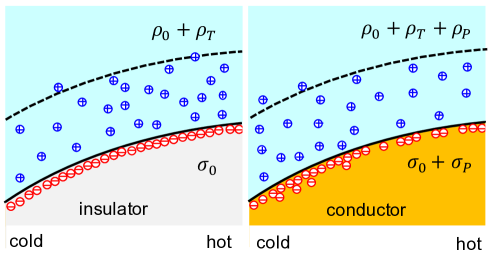
Figure 2: Electric double-layer in a thermal gradient (temperature increases from left to right). The left panel shows an insulating material. The surface charge density $\sigma_{0}$ is not affected by the Seebeck effect, whereas the diffuse layer comprises the non-uniform thermocharge density $\rho_{T}$. Its absolute value $|\rho_{T}|$ is proportional to the excess surface temperature, and its sign depends on the Seebeck coefficient; we show the case $S<0$. At a conducting surface (right panel), the parallel component of the electric field vanishes. The condition (24) requires a polarization charge $\sigma_{P}$ which induces a corresponding displacement of counterions $\rho_{P}$. Thus the diffuse layer consists of the counterions of $\sigma_{0}$ and $\sigma_{P}$, and of the thermocharge $\rho_{T}$. For typical parameters, these contributions satisfy $|\rho_{T}|\ll|\rho_{P}|\ll|\rho_{0}|$.

III.4 Charged conducting surface

Now we turn to conducting surfaces, such as the gold cap of the upper hemisphere in Fig. 1c. The electrostatic boundary conditions impose a constant potential, or a vanishing parallel electric field And06 , whereas at the outer boundary $z=B$, it is given by the Seebeck far-field:

$$E_{\parallel}(0)=S\nabla_{\parallel}T_{S}-\nabla_{\parallel}\varphi_{\sigma_{C}}(0)=0,\;\;\;\;\;\mathbf{E}(B)=S\mathbf{\nabla}T.$$ (24)

These conditions cannot be satisfied with the constant surface charge $-\sigma_{0}$ discussed so far.

To achieve (24) the mobile electrons in the metal surface move until their polarization charge density $\sigma_{P}$ results in a constant surface potential. The polarization charge is determined by inserting $\varphi_{\sigma}$ with

$${\sigma_{C}}(x)=\sigma_{T}(x)+\sigma_{0}+\sigma_{P}(x)$$ (25)

in Eq. (24) and solving for $\sigma_{P}$. Assuming that the total charge does not change, one has for the surface integral $\left<\sigma_{P}\right>=S^{-1}\int dS\sigma_{P}=0$. Its derivation is given in Appendix C. Its overall behavior is illustrated by the simpler expression (84) obtained in Debye-Hückel approximation,

$$\sigma_{P}=\frac{\varepsilon S(T_{S}-\left<T_{S}\right>)}{\lambda},\;\;\;\;\;\;(\mathrm{DHA}).$$ (26)

The polarization charge varies along the surface and even changes sign. For a negative Seebeck coefficient, one has $\sigma_{P}<0$ at the hot end of the metal surface, and $\sigma_{P}>0$ at the cold end, as shown in Fig. 2b.

Since the diffuse layer screens the local surface charge density, $\sigma_{P}$ induces a corresponding change of the mobile charge density, $\rho_{P}$, and we have $\rho_{C}=\rho_{T}+\rho_{0}+\rho_{P}$. We recall that the double-layer potential $\varphi_{\sigma}$ is calculated with the parameter $\sigma_{C}$ which accounts for the charge density of the diffuse layer, $\sigma_{C}=\int dz\rho_{C}(z)$, whereas the surface charge density is given by $-(\sigma_{0}+\sigma_{P})$. Accordingly, we have

$$E_{\bot}(0)=-\frac{\sigma_{0}+\sigma_{P}}{\varepsilon}$$ (27)

at the particle surface.

The parallel field component of the electric field,

$$E_{\parallel}(z)=S\mathbf{\nabla}_{\parallel}T_{S}-\mathbf{\nabla}_{\parallel}\varphi_{\sigma_{C}}(z),$$ (28)

is zero at the particle surface. With increasing distance, the double-layer potential $\varphi_{\sigma}$ decays and vanishes well beyond the screening length, and the electric field is given by (5). The overall behavior is best displayed in Debye-Hückel approximation,

$$E_{\parallel}(z)=S\mathbf{\nabla}_{\parallel}T_{S}\left(1-e^{-z/\lambda}\right),\;\;\;\;(\mathrm{DHA}).$$ (29)

This expression satisfies both the surface and far-field boundary conditions (24). The crossover occurs at the scale of the Debye length and results from the polarization charge $\sigma_{P}$, whereas the far-field is related to the thermocharge $\sigma_{T}$.

IV Non-equilibrium double-layer and creep flow

In the absence of interactions between the electrolyte solution and the boundaries, the stationary state is characterized by a salt gradient, a Seebeck field, and thermocharges at the boundaries, but there is no flow or electric current; compare the steady state obtained in Sect. II. Now we turn to interacting surfaces, more precisely to charged boundaries with an electric double layer, and we derive the creep flow along the surface. We linearize in the gradients of the non-equilibrium state; this implies that we do not consider the coupling of the Seebeck field with the thermocharge.

IV.1 Thermodynamic forces and slip velocity

Closely following Ref. Wue10 , we derive how the electric double layer of the surface interacts with the temperature gradient and its companion fields. Novel results arise from the coupling of the diffuse layer with the Seebeck field. We start from the well-known expression for the effective slip velocity Der41 ; And89 ,

$$v_{s}=\frac{1}{\eta}\int_{0}^{\infty}dzzf_{\parallel},$$ (30)

where $\eta$ is the solvent viscosity and $f_{\parallel}$ the parallel component of the thermodynamic force density arising from the non-equilibrium state.

The force acting on a unit volume of the electric double layer comprises the divergency of the Maxwell tensor $\mathcal{T}$ and the gradient of the osmotic pressure $P$,

$$\mathbf{f}=\mathbf{\nabla}\cdot\mathcal{T}-\mathbf{\nabla}P.$$ (31)

The former accounts for the electric energy of the double layer; the resulting force

$$\mathbf{\nabla}\cdot\mathcal{T}=\rho\mathbf{E}-\frac{1}{2}E^{2}\mathbf{\nabla}\varepsilon=\rho(S\mathbf{\nabla}T-\mathbf{\nabla}\varphi_{\sigma})-\frac{1}{2}E^{2}\mathbf{\nabla}\varepsilon,$$ (32)

consists of the Coulomb force on the diffuse layer and the change in electric energy due to a permittivity gradient Str41 ; Lan87 ; Fay08 . The second equality separates the double-layer and Seebeck contributions to the Coulomb force.

The second term in (31) stems from the osmotic pressure $P=\delta nk_{B}T$ exerted by the excess ion concentration $\delta n$ in the double layer. Inserting (77) and evaluating the gradient, one needs to account for the variation with temperature, salinity, and the potential $\varphi_{\sigma}$, resulting in

$$\mathbf{\nabla}P=-\rho\mathbf{\nabla}\varphi_{\sigma}+(\rho\varphi_{\sigma}+\delta nk_{B}T)\frac{\mathbf{\nabla}T}{T}+\delta nk_{B}T\frac{\mathbf{\nabla}n}{n}.$$ (33)

In these relations for $\mathbf{\nabla}\cdot\mathcal{T}$ and $\mathbf{\nabla}P$, the potential $\varphi_{\sigma}$ varies rapidly in normal direction, and slowly along the surface. The quantities $T$, $\varepsilon$, and $n$ vary slowly in all directions, on the scale of the particle parameter, whereas the charge density $\rho$ and the ion density $\delta n$ vanish beyond the diffuse layer.

Gathering the different terms one obtains the force density

$$\mathbf{f}=\rho S\mathbf{\nabla}T-(\rho\varphi_{\sigma}+\delta nk_{B}T)\frac{\mathbf{\nabla}T}{T}-\delta nk_{B}T\frac{\mathbf{\nabla}n}{n}-\frac{1}{2}E^{2}\mathbf{\nabla}\varepsilon.$$ (34)

In addition to the temperature gradient, $\mathbf{f}$ depends on the gradients of salinity and permittivity, induced by the Soret effect and the temperature dependence of $\varepsilon$. In linear-response approximation, we replace the coefficients of the gradients in (34) by the corresponding equilibrium quantities, and the electric field in the last term by $-\nabla\varphi_{\sigma_{0}}$. The gradient fields in (34) are constant on the scale of the screening length, whereas the coefficients $\rho$, $\delta n$, and $E$ vanish well beyond the diffuse layer.

As a remarkable feature, the parallel gradient $\nabla_{\parallel}\varphi_{\sigma}$ has disappeared from the double-layer forces. While both the electrostatic force $\nabla\cdot\mathcal{T}$ and the pressure gradient $\nabla P$ depend on the precise form of the parameter $\sigma$, these terms cancel in (34), and so do the polarization contributions. With the Poisson-Boltzmann expressions for $\varphi_{\sigma}$ and its derivatives given in Appendix B, the integrals in (30) are readily performed Mor99 ; Wue08 ,

$$v_{s}=-\frac{\varepsilon\zeta}{\eta}S\nabla_{\parallel}T+\frac{\varepsilon(\zeta^{2}-3\zeta_{T}^{2})}{2\eta}\frac{\nabla_{\parallel}T}{T}-\frac{\varepsilon\zeta_{T}^{2}}{2\eta}\left(\frac{\nabla_{\parallel}\varepsilon}{\varepsilon}+\frac{\nabla_{\parallel}n}{n}\right),$$ (35)

with the surface potential $\zeta=\varphi_{\sigma_{0}}(0)$ and the quantity $\zeta_{T}=(2k_{B}T/e)[\ln\cosh(e\zeta/4k_{B}T)^{2}]^{1/2}$. Each term of the slip velocity consists of a gradient field characterizing the non-equilibrium state of the electrolyte solution, and a coefficient that depends on the equilibrium properties of the solid surface and of the electrolyte solution. With the bulk salinity gradient $\nabla n$ as defined in (3) and the logarithmic permittivity derivative $\tau=-d\ln\varepsilon/d\ln T$, one has

$$\frac{\nabla_{\parallel}n}{n}=-S_{T}{\nabla_{\parallel}T},\;\;\;\;\;\frac{\nabla_{\parallel}\varepsilon}{\varepsilon}=-\tau\frac{\nabla_{\parallel}T}{T},$$

where $\tau\approx 1.5$ at room temperature Cat03 . A temperature gradient of Kelvin per micron results in a velocity of micron per second.

At a surface in a constant external temperature gradient $\nabla T$, the parallel component is simply given by its projection on the surface; for a spherical particle one has $\nabla_{\parallel}T=\sin\theta\nabla T$, with the polar angle $\theta$ and where we have discarded corrections due to the thermal conductivity contrast; see Eq. (42) below. The self-generated temperature field of a laser-heated particle results in a more complex expression, depending on its absorption coefficient and thermal conductivity Bic13 . The surface potential $\zeta$ usually depends weakly on temperature; the variation of $v_{s}$ is rather irrelevant except for Janus particles with different $\zeta$ on the two hemispheres; the surface potential could even take opposite signs on the metal cap and on the insulating half.

The novel result concerns the thermoelectric contribution to (35), that is, the first term proportional to the electrolyte Seebeck coefficient $S$. The remaining term $\propto\nabla T$ and that $\propto\nabla\varepsilon$ are known as thermo-osmosis Der41 ; Bre16 , whereas the last one, $\propto\nabla n$, is similar to salt osmosis Pri87 ; Abe09 . As a main finding of this work, we note that $v_{s}$ does not depend on the electrical conductivity of the particle surface. The slip velocity is the same for insulating and conducting materials, although the electric field at the surface shows quite a different behavior: Its parallel component is finite at an insulating surface but vanishes at a conductor, as shown by Eqs. (23) and (29), respectively. A similar effect was shown to occur for the electrophoretic mobility at a metal surface Squ04 , resulting in an electroosmotic slip velocity that is the same at insulating and conducting surfaces.

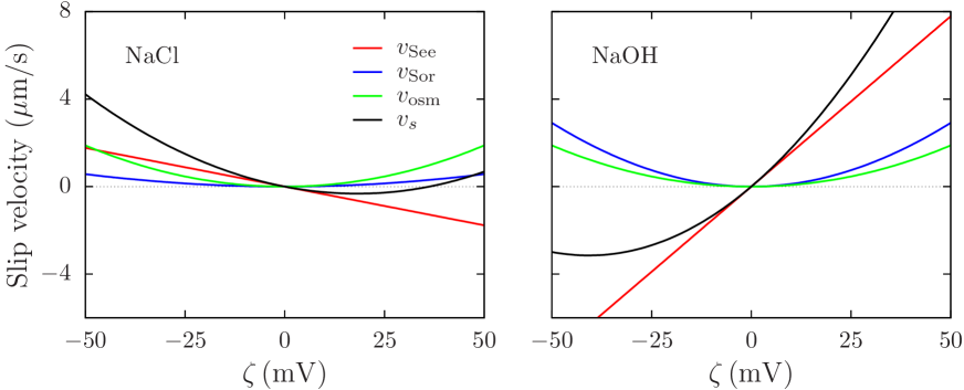
Figure 3: Comparison of the different contribution to the slip velocity (36) for NaCl and NaOH solutions, as a function of the $\zeta$-potential. We plot separately the Seebeck, Soret, and thermoosmotic contributions, as defined in (36). For NaCl and NaOH solutions, the Seebeck coefficient takes the values $S=-0.2\,\textrm{mV/K}$ and $S=0.05\,\textrm{mV/K}$, respectively; for the Soret coefficent one has $S_{T}=2.7\times 10^{-3}\,\textrm{K}^{-1}$ and $1.4\times 10^{-2}\,\textrm{K}^{-1}$. We use the temperature gradient $\nabla_{\parallel}T=1\,\mathrm{K/\mu m}$, the viscosity and permittivity of water, and ambient temperature.

IV.2 Relevance of ion-specific contributions

In order to compare their relative importance, we plot in Fig. 3 the different contributions to the slip velocity, for parameters describing NaCl and NaOH solutions. With a temperature gradient of 1K/$\mu$m, which is easily achieved by heating gold microstructures, one finds velocities of the order of microns per second. We split the slip velocity (35) in three terms,

$$v_{\mathrm{See}}=-\frac{\varepsilon\zeta}{\eta}S\nabla_{\parallel}T,\;\;\;\;v_{\mathrm{Sor}}=\frac{\varepsilon\zeta_{T}^{2}}{2\eta}S_{T}{\nabla_{\parallel}T},\;\;\;\;v_{\mathrm{osm}}=\frac{\varepsilon[\zeta^{2}-(3-\tau)\zeta_{T}^{2}]}{2\eta}\frac{\nabla_{\parallel}T}{T},$$ (36)

where the first and second ones are proportional to the Seebeck and Soret coefficients, and the third one describes the velocity induced by heat flow or “thermoosmosis”. This thermoosmotic velocity $v_{\mathrm{osm}}$ is dominant in the absence of salt Der41 ; Bre16 . In the presence of salt, however, the Seebeck and Soret velocities exceed thermoosmosis; experiments on nanometric micelles Vig10 and micrometric polystyrene particles Esl14 provide conclusive evidence for magnitude of the ion-specific Seebeck and Soret contributions. The data of Ref. Esl14 indicate that both $S$ and $S_{T}$ strongly depend on temperature.

Note that the Seebeck term is linear in the surface potential $\zeta$ and thus takes opposite signs at positively and negatively charged surfaces. All other contributions to $v_{s}$ are quadratic in $\zeta$. The self-propulsion velocity $u$ of a Janus particle is given by the surface average of the slip velocity, $\mathbf{u}=-\left<(1-\mathbf{n}\mathbf{n})\cdot\mathbf{v}_{s}\right>$, with the surface normal $\mathbf{n}$ And89 .

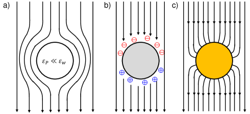
Figure 4: Electric field lines for insulating and conducting particles. a) Electric field due to an applied external voltage. The field does not penetrate in a low-permittivity particle ($\varepsilon_{P}\ll\varepsilon_{w}$), resulting in a characteristic deformation. b) Thermoelectric field in the vicinity of an insulating particle. The field is not deformed by the permittivity contrast but follows the temperature gradient, $E=S\nabla T$. (For the sake of simplicity we assume constant $\nabla T$, that is, similar thermal conductivities of particle and solvent.) Within one Debye layer from the particle surface, its normal component $E_{\perp}$ is screened by ion accumulation, that is, the thermocharge $\rho_{T}$, as shown in the left panel of Fig. 2; the parallel component $E_{\parallel}$ does not vanish, and the particle surface is not at constant potential. c) Thermoelectric field in the vicinity of a conducting particle. Polarization of the metal surface adjusts the surface charge density such that the parallel component of the field vanishes, resulting in an isopotential surface; $\sigma$ is illustrated in the right panel of Fig. 2.

V Discussion

Here we discuss the main features of the thermocharge and the thermoelectric field, and their dependence on material properties such as electric conductivity, surface roughness, and heat conductivity.

V.1 Seebeck field in the vicinity of a spherical particle

The Seebeck field does not result from an externally applied voltage but from thermocharges at the hot and cold boundaries which, in turn, are due to the thermal forces (1) on the ions, as shown schematically in Fig. 1b for a Janus particle. At first sight one would expect that a thermoelectric field and an external field show the same behavior in the vicinity of a colloidal sphere. After all, both are subject to the same electrostatic boundary condition at the particle surface. It turns out, however, that their behavior is quite different. In Fig. 4 we compare their field lines around a spherical particle. For the sake of clarity we discuss the case of an external constant temperature gradient; the same physical effects occur for the self-generated gradient of a heated Janus particle or for a hot metal nanostructure.

The left panel of Fig. 4 shows the well-known deformation of an external electric field $E_{0}$ in the vicinity of a low-permittivity particle. The parallel field at the surface varies as

$$E_{\parallel}=\frac{3}{2}E_{0}\sin\theta$$ (37)

with the polar angle $\theta$ And89 . With respect to the bulk field, it is enhanced by the permittivity ratio of particle and solvent, $3\varepsilon_{w}/(2\varepsilon_{w}+\varepsilon_{P})\approx\frac{3}{2}$.

The Seebeck field, on the contrary, results from surface charges; in order to satisfy the electric boundary condition for its normal component, it accumulates mobile ions with one screening length at the particle surface. The middle panel of Fig. 4 shows the thermoelectric field lines. They are not deformed and end at the thermocharge accumulated at the particle surface. The parallel component reads as

$$E_{\parallel}=S\nabla_{\parallel}T\sin\theta.$$ (38)

Contrary to an external field, the surface field is not enhanced by the permittivity contrast.

The right panel shows the deformation of the Seebeck field by a conducting particle, where the parallel component of the surface field vanishes, $E_{\parallel}=0$. From a comparison of the three situations shown, it is clear that the behavior of the thermoelectric field at solid boundaries significantly differs from that of a voltage induced field.

The resulting electric field lines of a heated Janus particle are shown in Fig. 1b: The far-field corresponds to the Seebeck field (5), whereas the near-field depends on the surface properties, as illustrated in Fig. 1c for the conducting and insulating hemispheres. The near-field corresponds to a superposition of the situations shown in Figs. 4 b and c.

V.2 Thermocharge

The thermocharge arises from the thermal forces $H_{\pm}\nabla T/T$ which drive the ions towards the hot or cold boundaries. When solving, in the simplest case, the zero-current condition (7) and Gauss’ law (8), one finds that the steady state is characterized by a thermoelectric field and surface charges. The thermocharge per unit area $\sigma_{T}$, is independent of the material properties of the surface and of its surface charge $\sigma_{0}$. The profile of the diffuse layer, however, does depend on $\sigma_{0}$: At an uncharged surface, $\sigma_{0}=0$, it follows the exponential law $\rho_{T}=\sigma_{T}e^{-z/\lambda}$, whereas at a strongly charged surface, $\rho_{T}$ is part of the diffuse layer of Poisson-Boltzmann theory given in Eq. (70).

According to Eq. (12), the thermocharge is entirely determined by the normal component of the temperature gradient at the solid surface and the Seebeck coefficient of the electrolyte,

$$\sigma_{T}=\varepsilon S\nabla_{\perp}T_{S}.$$ (39)

On a sphere, the gradient is given by the local excess temperature and the radius, $\nabla_{\perp}T_{S}=-(T_{S}-T_{0})/a$. In the case of a non-uniformly heated Janus particle, the temperature $T_{S}$ varies along the surface, and so does the charge per unit area $\sigma_{T}$, as illustrated in Fig. 1b. A positive Seebeck coefficient, e.g., for aqueous solutions of NaCl, results in a negative $\sigma_{T}$, whereas a positive surface charge occurs for $S<0$ as, e.g., in NaOH solution.

As an estimate of its order of magnitude, we calculate the thermocharge density per unit area, $\sigma_{T}$, for a micron-size particle with an excess temperature of 30 K and the Seebeck coefficient of NaOH, $S=-200\,\mu\text{V/K}$,

$$\sigma_{T}\sim 10^{-5}\,e/\mathrm{nm}^{2}.$$ (40)

For comparison, the bare charge of a colloidal particle is of the order $\sigma_{0}\sim e/\mathrm{nm}^{2}$.

V.3 Polarization charge on a conducting surface

The thermocharge discussed above, is the same on insulating and conducting surfaces. On the latter, however, the isopotential condition of electrostatics imposes a polarization charge of the metal coating. Like any surface charge of a solid boundary, the polarization charge is screened by its counterions. In other words, the polarization of the electronic system induces a corresponding polarization of the diffuse layer, as illustrated in right panel of Fig. 2. Thus the polarization effects concern only the immediate vicinity of the particle. Well beyond the Debye length, the effect of the polarization charges vanishes. Accordingly, the field lines of insulating and conducting particles in Fig. 4b and c, differ within the screening length, but are identical at larger distances.

For an excess temperature of 30 K, the Seebeck coefficient $S=-200\,\mu\text{V/K}$, and $\lambda=2$ nm, the weak-coupling expression (26) gives the order-of-magnitude estimate

$$\sigma_{P}\sim 10^{-2}e/\mathrm{nm}^{2}.$$ (41)

When comparing with the thermocharge, one finds that $\sigma_{P}$ exceeds $\sigma_{T}$ by a factor $a/\lambda$ which, for micron-size particles, is of the order of $a/\lambda\sim 1000$. On the other hand, the polarization charge may attain several percent of the colloidal surface charge $\sigma_{0}$.

As a related quantity we estimate the thermopotential $\varphi_{T}=-S(T_{S}-T_{0})$. The above parameters give $\varphi_{T}\sim 6$ mV, which is almost comparable to the surface potential of moderately charged colloids, $\zeta\sim 30$ mV. One should note, however, that the variation of $\varphi_{T}$ is a more relevant quantity than its absolute value. Still, for a typical temperature profile, one finds the thermopotential at the two poles of a Janus particle differs by about half of its mean value.

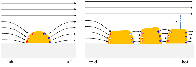
Figure 5: Schematic view of the thermoelectric field and polarization charges of gold grains at a low-permittivity insulating surface, in contact with an electrolyte solution with positive Seebeck coefficient, $S>0$. The left panel shows the case of single grain. The field is normal at the grain surface because of the electrostatic boundary conditions, and parallel at the insulating solid, because of the strong permittivity contrast of its material and water. Well beyond the screening length one recovers the constant Seebeck far-field. The right panel shows a densely covered surface, where each grain forms an equipotential surface and carries opposite polarization charges $\sigma_{P}$ at its cold and hot sides.

V.4 Granular gold surface

So far we considered a continuous gold surface, as shown in Fig. 1c. Yet this does not always correspond to the actual experimental situation. For example, the cap of the Janus particles used in Ref. Sim16 consists of a dense coverage of nano-sized gold grains, visible in scanning electron microscopy images Ned15 . Since the grains are not connected, the active cap of these particles does not form an isopotential surface, contrary to what we assumed so far.

Here we give a qualitative discussion of the resulting Seebeck field and slip velocity. From our results for conducting surfaces, it is clear that the parallel component of the thermoelectric field is screened within one screening length. Fig. 5 gives a schematic view of an insulating surface, partly covered by gold grains and at a non-uniform temperature. According to the discussion in Sect. V.6 below, we neglect the thermal conductivity contrast. On the other hand, gold nanostructures keep their electric conductivity, though it is lower than that of bulk material; thus the grains are conducting and that each of them forms an equipotential surface.

The left panel of Fig. 5 shows the thermoelectric properties of a single grain. The parallel component of the Seebeck far-field induces polarization charges, such that isopotential condition is satisfied at the surface. For a gold hemisphere mounted on a low-permittiivity material, the resulting electric field and polarization charges are obtained from Appendix A.3 by retaining the term $c_{1}$ only. Note that beyond a distance of one screening length, one recovers the macroscopic thermoelectric field. The right panel of Fig. 5 shows a densely covered surface, where the distance between grains does not exceed the screening length. Then the overall thermopotential is split in small jumps between nearby grains; their cold and hot boundaries carry polarization charges which result in a strong electric field in the spacing. The field component parallel to the surface vanishes at the grain surface but increases beyond and tends towards the far-field value beyond double layer.

The slip velocity is essentially determined by the layer of thickness $\lambda$ above the gold grains, whereas the narrow space between the grains is of little relevance. A different picture would arise if the gold grains covered only a small fraction of the surface, and if their height was small as compared to their spacing. For a situation as shown by Fig. 5 or by the electron micrograph in Ref. Ned15 , however, we conclude that the picture developed for micron-size conducting surfaces remains at least qualitatively correct for a granular gold coating. Because of the surface roughness one may expect a somewhat modified slip velocity, probably smaller than at a homogeneous cap.

V.5 Comparison with experiment

So far there are few direct measurements of the slip velocity with respect to a wall Der41 ; Bre16 ; most experiments report the motion of dispersed particles in an external temperature gradient Bra13 ; Lin17 ; Lin17b ; Put05 ; Vig10 ; Esl14 or of self-propelling microswimmers Jia10 ; Bar13 ; Sim16 ; But12 , where the velocity is given by the surface average of the slip velocity.

The slip velocity (35) consists of various contributions, proportional to the temperature gradient and its companion fields. All of them are of comparable magnitude. The slip velocity varies as a function of the electrolyte strength and, through the Soret and Seebeck coefficients, depends on specific-ion properties. At room temperature, the Soret coefficient $S_{T}$ is usually positive Nak88 . Then except for the Seebeck contribution, all terms of the slip velocity are positive, and the boundary layer flows towards the hot. There is, however, strong evidence that the Seebeck term is dominant for common salt and buffer solutions, such as NaCl, NaOH, citric acid, and CAPS. Since their Seebeck coefficients take opposite signs, one observes, as a most striking feature, a positive slip velocity for NaCl Esl14 and a negative one for NaOH Vig10 ; Esl14 ; thus changing the anion reverses the direction of thermally driven motion. Similar effects were reported for buffer solutions Put05 .

The main results of the present paper concern the slip velocity along metal surfaces. Though local heating of gold structures is widely used for manipulating of particles and cells Bra13 ; Lin17 ; Lin17b ; Lin17a or powering microswimmers Jia10 ; Bar13 ; Sim16 ; But12 ; Gir16 , there is at present no systematic study of the creep flow along a conducting surface. Evidence for thermo-electric driving of hot silica particles with a granular gold cap, was reported by one recent experiment Sim16 : Probing the particle’s self-propulsion velocity in 10 mM solutions of NaCl, LiCl and NaOH, revealed a salt-specific effect, which agrees qualitatively with the Seebeck coefficients of these electrolytes, $S_{\text{NaCl}}>S_{\text{LiCl}}>S_{\text{NaOH}}$. Since the thermophoretic self-propulsion is superposed on motion due to radiation pressure and gravity, these data do not provide an absolute measure of $v_{s}$, but only qualitative differences upon changing the ions. In summary, the data of Ref. Sim16 confirm the existence of an electrolyte Seebeck effect for active Janus particles, yet they do not provide clear evidence whether the thermoelectric driving is the same on the silica and gold hemispheres, as suggested by the present work, or whether the Seebeck effect vanishes on the metal surface.

V.6 Temperature gradient at the particle surface

Throughout this paper we have assumed that the temperature gradient is not modified at the solid-water interface, which is justified as long as the heat conductivities of liquid and particle, $\kappa_{w}$ and $\kappa_{P}$, take similar values. For a sufficiently strong conductivity contrast, however, the particle deforms the temperature field in its vicinity. For a sphere, a conductivity contrast modifies the parallel and perpendicular components of the temperature gradient according to

$$\nabla_{\parallel}T_{S}\rightarrow\xi_{\parallel}\nabla_{\parallel}T_{S},\;\;\;\;\;\nabla_{\perp}T_{S}\rightarrow\xi_{\perp}\nabla_{\perp}T_{S},$$ (42)

with the well-known constants Wue10

$$\xi_{\parallel}=\frac{3\kappa_{w}}{2\kappa_{w}+\kappa_{P}},\;\;\;\xi_{\perp}=\frac{3\kappa_{P}}{2\kappa_{w}+\kappa_{P}}.$$ (43)

In order to account for the conductivity contrast in the results of the preceding sections, one merely has to introduce these factors. Typical insulating materials, like silica and polystyrene, show a somewhat lower heat conductivity than water. The most important thermoelectric properties are proportional to parallel gradient, with a correction factor $\xi_{\parallel}$ between 1 and $\frac{3}{2}$, which is usually of little relevance.

A more complex situation occurs for thin metal coatings. Metals conduct heat much better than water, $\kappa_{m}\gg\kappa_{w}$. A metal coating of thickness $d$ significantly deforms the temperature profile of a sphere of radius $a$, if the conductivity contrast satisfies $\kappa_{m}/\kappa_{w}>a/d$; in the thick-cap limit the metal surface becomes an isothermal Bic13 . Noting that $\kappa_{m}$ decreases for films of less than $100\,\mathrm{nm}$, one finds that for micron-size particles, the temperature is modified by coatings thicker than several tens of nanometer.

Most recent experiments are done on Janus particles with thinner coatings, of less than $10\,\mathrm{nm}$, where the cap contribution to heat conduction and the resulting deformation of the temperature field can be neglected. On the other hand, such thin gold coatings still have significant electrical conductivity, and thus develop polarization charges as discussed in this paper and shown in Figs. 2 and 4.

V.7 Transient and memory effects.

So far we have considered the steady-state Seebeck effect. The transient behavior after switching on the heat source is readily obtained from the advection-diffusion equation for the ions with Gauss’ law $\nabla\cdot E=\rho/\varepsilon$. Thus we find

$$\rho_{T}(t)=\rho_{T}(\infty)(1-e^{-t/\tau_{\text{ion}}}),$$ (44)

where the characteristic time scale expresses the time of ion diffusion over the screening length,

$$\tau_{\text{ion}}=\frac{\lambda^{2}}{2D}.$$ (45)

With typical values $D\sim 10^{-9}$ m²/s and $\lambda\sim 50$ nm, one finds $\tau\sim\mu$s.

Thus building up the Seebeck field requires a few microseconds, and the same time-dependence occurs for the slip velocity. Indeed, the thermal and hydrodynamic time scales, $\tau_{\text{th}}=\lambda^{2}/\alpha$ and $\tau_{\text{hy}}=\lambda^{2}/\nu$, are by several orders of magnitude shorter, since both heat diffusivity ($\alpha\sim 10^{-7}$ m²/s) and kinematic viscosity ($\nu\sim 10^{-6}$ m²/s), by far exceed ion diffusivity. It should be noted that $\tau_{\text{hy}}$ is much shorter than the hydrodynamic memory of Brownian motion, $\tau_{\text{hy}}^{\prime}=a^{2}/\nu$ Fra11 ; this is due to the fact that in the latter case, the hydrodynamic stress decays over the particle size $a$, whereas for phoretic and active particles, the relevant stress is confined within the interaction length $\lambda$ Fay08 .

As a consequence, we expect a rather intricate behavior of the particle motion during the first milliseconds,

$$v_{s}(t)=v_{s}^{\text{el}}(1-e^{-t/\tau_{\text{ion}}})+v_{s}^{\text{osm}}(1-e^{-t/\tau_{\text{th}}}),$$ (46)

where the thermo-electric slip velocity $v_{s}^{\text{el}}$ corresponds to the first term of (35), and the osmosis-driven one $v_{s}^{\text{osm}}$ to the remainder. The latter sets in on the heat-diffusion time scale $\tau_{\text{th}}\sim 10$ nanoseconds. The Seebeck effect requires ion diffusion which occurs on the time scale $\tau_{\text{ion}}$ that may attain a microsecond. Since in many instances, the thermoelectric slip velocity $v_{s}^{\text{el}}$ is stronger and carries the opposite sign Put05 ; Vig10 ; Esl14 , the onset of the Seebeck effect could even result in a reversal of the direction of motion.

The above discussion applies to the double-layer at the conducting hemisphere, where the local temperature gradient is determined by absorption of laser light by the gold coating. At the insulating hemisphere, building up the stationary temperature profile requires heat diffusion over a distance comparable to the particle radius. Thus the thermal time scale, $\tau_{\text{th}}^{\text{ins}}=a^{2}/\alpha$, is of the order of ten microseconds, which is close to the ionic relaxation time $\tau_{\text{ion}}$. Thus on an insulating surface, the time scales of the two terms in the slip velocity (46) are not very different.

VI Summary

We find that hot metal structure in contact with an electrolyte solution, show thermoelectric properties at the nanoscale that depend both on surface material properties and ion-specific effects. Here we briefly summarize our main results.

The diffuse layer comprises a thermocharge $\rho_{T}$ which is proportional to the surface temperature $T_{S}$. On a Janus particle, $T_{S}$ increases from the passive hemisphere to the heated cap, and so does the thermocharge, resulting in a parallel component of the Seebeck field along the particle surface.

On a conducting surface, such as a gold cap, however, the parallel temperature gradient induces a polarization charge on the metal structure, which modifies the double layer such that the parallel component of the electric field vanishes at the surface. Yet this does not affect the thermally induced slip velocity, which turns out to be identical on insulating and conducting surfaces.

In previous work the Seebeck field had been considered like a field due to an external voltage. We find that the near-field is rather different, as shown in Figs. 3 a and b. As a consequence, the parallel field at a spherical particle (38) does not carry a factor $\frac{3}{2}$, contrary to an external field (37) at a low-permittivity particles. The same difference occurs between the thermoelectric contribution to the slip velocity (35) and the electroosmotic velocity.

Regarding specific-ion effects, our findings agree qualitatively with a recent experiment on gold-capped silica particles, showing a significant variation of the self-propulsion velocity with the used salts NaOH, NaCl, LiCl Sim16 . The data do not provide conclusive evidence for thermoelectric driving along the metal cap.

From our analysis of the onset of thermoosmotic and thermoelectric driving, we expect striking transient effects. Because of the slow diffusion of ions, as compared to diffusion of heat and momentum, the thermo-electric slip velocity sets in on a microsecond timescale. The much faster onset of thermoosmosis, should result in a two-step transient behavior upon switching on the heating.

AL and AW acknowledge support by the French National reasearch agency through contract ANR-13-IS04-0003. AW thanks Frank Cichos and Martin Fränzl for stimulating discussions.

Appendix A Thermocharge of an uncharged particle

Here we derive in detail the thermocharge of an uncharged spherical particle. Since the thermocharge is small, we may resort to Debye-Hückel approximation, and for the spherical geometry, the thermoelectric potential can be given explicitly in terms of a multipole expansion. We first provide the general formulae for weak coupling, evaluate them for a 1D geometry, and then consider insulating and conducting particles with non-uniform surface temperature.

A.1 Debye-Hückel theory

Here we derive the thermocharge of an uncharged hot particle in some more detail than in the main text. We start from the relation between thermocharge density $\rho$ and thermoelectric field $\mathbf{E}$ obtained in Sect. II,

$$\nabla\rho+\frac{\varepsilon}{\lambda^{2}}(S\mathbf{\nabla}T-\mathbf{E})=0.$$ (47)

This equation has two solutions, and the electrostatic potential consists of two contributions accordingly,

$$\varphi=\varphi_{T}+\varphi_{\sigma}.$$ (48)

The first one, $\mathbf{E}_{T}=S\mathbf{\nabla}T$ and $\rho=0$, corresponds to the far-field (5) with zero charge density and the thermoelectric potential

$$\varphi_{T}=-S(T-T_{0}),$$ (49)

whereas the second solution is given by the screened Debye-Hückel potential $\varphi_{\sigma}$. Indeed, completing $\nabla\rho=(\varepsilon/\lambda^{2})\mathbf{E}$ with Gauss’ law $\rho=\varepsilon\text{div}\mathbf{E}$, one finds $\mathbf{E}=-\mathbf{\nabla}\varphi_{\sigma}$, where $\varphi_{\sigma}$ solves the Debye-Hückel equation

$$\nabla^{2}\varphi_{\sigma}=\frac{\varphi_{\sigma}}{\lambda^{2}}.$$ (50)

A.2 1D geometry

These equations have been solved previously for a 1D geometry between a hot and a cold plate Maj11 , and for a uniformly heated spherical particle Maj12 . With the constant temperature gradient $\nabla T$ along the $z-$direction, one readily calculates the Seebeck field,

$$E=S\nabla T\left(1-\frac{\cosh(z/\lambda)}{\cosh(L/2\lambda)}\right),$$ (51)

where $-L/2\leq z\leq L/2$. If the system size $L$ is much larger than the Debye length $\lambda$, one has the bulk field $E=S\nabla T$; at the boundaries, $E$ is exponentially screened and vanishes at the hot and cold surfaces.

The corresponding thermocharge at the boundaries is given by Gauss’ law,

$$\rho_{T}=\varepsilon\partial_{z}E=-\varepsilon S\nabla T\frac{\sinh(z/\lambda)}{\cosh(L/2\lambda)}.$$ (52)

For $L\gg\lambda$, this simplifies to $\rho_{T}=\mp\varepsilon S\nabla Te^{(\pm z-L/2)/\lambda}$, resulting in positive and negative charge layers at the hot and cold boundaries.

A.3 Spherical particle

For a spherical particle, the inhomogeneous solution (49) is given by a multipole expansion for the temperature field,

$$T(\mathbf{r})=T_{0}+\sum_{n=0}^{\infty}t_{n}P_{n}\left(c\right)\frac{a^{n+1}}{r^{n+1}},$$ (53)

where $c=\cos\theta$ is the cosine of the polar angle. The mean excess surface temperature $t_{0}=q/4\pi\kappa a$ is determined by the rate of heat absorption $q$, the thermal conductivity of the solvent $\kappa$, and the particle radius $a$.

The homogeneous solution $\varphi_{\sigma}$ is obtained as a series

$$\varphi_{\sigma}=\sum_{n=0}^{\infty}c_{n}P_{n}\left(c\right)\frac{k_{n}\left(r/\lambda\right)}{k_{n}\left(a/\lambda\right)},$$ (54)

in terms of Legendre polynomials $P_{n}\left(c\right)$ with $c=\cos\theta$, and the modified spherical Bessel function of the second kind $k_{n}\left(x\right)$. For the sake of notational convenience, we introduce the factor $k_{n}\left(a/\lambda\right)$, such that the radial solutions are normalized at the particle surface $r=a$.

A.4 Insulating particle

The coefficients $c_{n}$ of the homogeneous solution remain to be determined from the electrostatic boundary conditions at the particle-water interface. For a low-permittivity material we may put $\varepsilon_{P}/\varepsilon_{w}\rightarrow 0$. Then the boundary conditions require that the normal component of the electric field vanishes,

$$E_{\bot}(r=a)=0.$$ (55)

Taking the radial derivative of $\varphi$, putting $r=a$, and rearranging terms we find

$$c_{n}=St_{n}(n+1)\frac{\lambda}{a}\frac{k_{n}\left(a/\lambda\right)}{k_{n}^{\prime}\left(a/\lambda\right)}.$$

with the dimensionless derivative $k_{n}^{\prime}\left(x\right)=\partial_{x}k_{n}(x)$.

These coefficients determine the thermopotential $\varphi$. In order to simplify the resulting expressions we note that the ratio of Debye length $\lambda$ and particle radius $a$ is at most of the order of a few percent. Expanding in powers of the small parameter $\lambda/a$,

$$\frac{k_{n}\left(r/\lambda\right)}{k_{n}\left(a/\lambda\right)}=\frac{a}{r}e^{\left(a-r\right)/\lambda}\left[1+\frac{\lambda}{a}\frac{n\left(n+1\right)}{2}\left(1-\frac{a}{r}\right)+...\right],$$

we find that the first terms of the series are well approximated by

$$\frac{k_{n}\left(r/\lambda\right)}{k_{n}\left(a/\lambda\right)}\approx\frac{a}{r}e^{\left(a-r\right)/\lambda}\ \ \ \ (n<\sqrt{a/\lambda}).$$

In the most relevant near-field range, this approximation is even valid for $n<a/\lambda$. To leading order in the small parameter $\lambda/a$, we have $k_{n}^{\prime}\left(a/\lambda\right)/k_{n}\left(a/\lambda\right)=-1+O(\lambda/a)$. Then the above coefficient simplifies according to

$$c_{n}=St_{n}(n+1)\frac{\lambda}{a},$$ (56)

and the electrostatic potential reads as

$$\varphi=-S\sum_{n}t_{n}P_{n}(c)\left(\frac{a^{n+1}}{r^{n+1}}-(n+1)\frac{\lambda}{r}e^{\left(a-r\right)/\lambda}\right).$$ (57)

The screened term is by a factor $\lambda/a$ smaller than the first one; yet their radial derivatives cancel each other at $r=a$, thus satisfying (55).

The normal component of the electric field reads, to leading order in $\lambda/a$,

$$E_{\perp}(\mathbf{r})=S\nabla_{\perp}T(\mathbf{r})(1-e^{(a-r)/\lambda}).$$ (58)

In the screened terms we have discarded factors of $a/r$, since they are close to unity in the range where the exponential function is finite. This explicits how the thermocharge screens the normal electric field. The parallel field component, on the contrary, is hardly affected by the thermocharge,

$$E_{\parallel}(\mathbf{r})=S\nabla_{\parallel}T(\mathbf{r})(1+O(\lambda/a)).$$ (59)

The thermocharge density follows from Gauss’ law, $\rho_{T}=-\nabla^{2}\varphi_{\sigma}$. With the same approximations as for the normal field component above, we have

$$\rho_{T}=\frac{\varepsilon}{\lambda}e^{\left(a-r\right)/\lambda}S\nabla_{\bot}T|_{S}.$$ (60)

Integrating over the radial coordinate we find the charge per unit area

$$\sigma_{T}=\int_{0}^{\infty}dr\rho_{T}=\varepsilon S\nabla_{\bot}T|_{S}.$$ (61)

Integrating over the particle surface gives the total charge

$$Q_{T}=-4\pi a\varepsilon St_{0},$$ (62)

which is determined by the isotropic component of the excess temperature.

A.5 Conducting particle

The thermocharge $\rho_{T}$ is the same as obtained above for an insulating particle. The boundary conditions, however, impose that the parallel component of the electric field vanishes, whereas the normal component is eventually compensated by a polarization charge density $\sigma_{P}$ of the surface $r=a$,

$$E_{\perp}=-\frac{\sigma_{P}}{\varepsilon},\;\;\;\;E_{\parallel}=0.$$ (63)

Writing the surface charge as a series $\sigma_{P}=\sum_{n}s_{n}P_{n}(c)$ and inserting the potential $\varphi$, we determine the coefficients $c_{n}$ and $s_{n}$ to leading order in $\lambda/a$,

$$c_{n}=St_{n},\;\;\;\;s_{n}=-\frac{\varepsilon St_{n}}{\lambda}\;\;\;\;\;\;(n>0).$$

The isotropic terms are particular because of charge conservation,

$$c_{0}=\frac{\lambda}{a}St_{0},\;\;\;\;s_{0}=0.$$

Then the electrostatic potential reads

$$\varphi=-St_{0}\frac{a-\lambda e^{\frac{a-r}{\lambda}}}{r}-S\sum_{n>0}t_{n}P_{n}(c)\left(\frac{a^{n+1}}{r^{n+1}}-e^{\frac{a-r}{\lambda}}\right).$$ (64)

Resorting to the same approximation as in the insulating case, we have

$$\varphi=-St_{0}\frac{a-\lambda e^{\frac{a-r}{\lambda}}}{r}-S(T_{S}-\left<T_{S}\right>)\left(1-e^{\frac{a-r}{\lambda}}\right),$$ (65)

with the surface temperature $T_{S}$ and its mean value $\left<T_{S}\right>$. The polarization charge is given by

$$\sigma_{P}=\frac{\varepsilon}{\lambda}S(T_{S}-\left<T_{S}\right>),$$ (66)

For the normal component of the electric field we find

$$E_{\perp}(\mathbf{r})=S\nabla_{\perp}T(\mathbf{r})-\frac{S(T_{S}-\left<T_{S}\right>)}{\lambda}e^{\frac{a-r}{\lambda}}.$$ (67)

In the screened terms we have discarded factors of $a/r$, since they are close to unity in the range where the exponential function is finite. This explicits how the thermocharge screens the normal electric field.

To linear order in the excess temperature, the parallel field component,

$$E_{\parallel}(\mathbf{r})=S\nabla_{\parallel}T\left(1-e^{\left(a-r\right)/\lambda}\right),$$ (68)

vanishes at the surface and tends to the Seebeck field well beyond the double layer.

The thermocharge density follows from Gauss’ law, $\rho_{T}=-\nabla^{2}\varphi_{\sigma}$. With the same approximations as for the normal field component above, we have

$$\rho_{P}=\frac{\varepsilon}{\lambda^{2}}e^{\left(a-r\right)/\lambda}S(T_{S}-\left<T_{S}\right>).$$ (69)

Appendix B Poisson-Boltzmann theory

Consider a charged surface in contact with an electrolyte solution. In mean-field theory, the electrostatic potential $\varphi_{\sigma}$ satisfies the Poisson-Boltzmann equation

$$\nabla^{2}\varphi_{\sigma}=-\frac{\rho}{\varepsilon}=\frac{k_{B}T}{e\lambda^{2}}\sinh\frac{e\varphi_{\sigma}}{k_{B}T}.$$ (70)

If the particle radius is much larger than the Debye screening length, the curvature of the surface can be neglected. Then the Laplace operator reduces to the second derivative with respect to the vertical coordinate $z$, and the potential is the 1D solution And06

$$\varphi_{\sigma}(z)=-\frac{2k_{B}T}{e}\ln\frac{1+ge^{-z/\lambda}}{1-ge^{-z/\lambda}},$$ (71)

with the shorthand notation

$$\hat{g}=ge^{-z/\lambda},\;\;\;\;g=\sqrt{1+\ell^{2}/\lambda^{2}}-\ell/\lambda.$$ (72)

The parameter $g$ is given by the ratio of the Gouy-Chapman length $\ell=e/(2\pi\ell_{B}|\sigma|)$ and the Debye length $\lambda=1/\sqrt{8\pi\ell_{B}n}$. With the Bjerrum length $\ell_{B}=e^{2}/(4\pi\varepsilon k_{B}T)$ one finds

$$\frac{\ell}{\lambda}=\frac{e}{2\pi|\sigma|\ell_{B}\lambda}=\frac{e\sqrt{8n\varepsilon k_{B}T}}{|\sigma|},$$ (73)

with the salinity $n$. In the following we assume that $\sigma$ is positive, corresponding to the usual situation of a negative surface charge $-\sigma$.

The electric field $E_{\perp}=-d\varphi/dz$ is perpendicular to the surface and reads

$$E_{\perp}=-\frac{\sigma}{\varepsilon}e^{-z/\lambda}\frac{1-g^{2}}{1-\hat{g}^{2}}.$$ (74)

At the particle surface, one readily verifies the relation $E(0)=-\sigma/\varepsilon$.

The charge density $\rho$ in the diffuse layer is given by the second equality in (70). An equivalent form in terms of the parameter $g$ is obtained from Gauss’ law $\rho=\varepsilon dE/dz$,

$$\rho=\frac{\sigma}{\lambda}e^{-z/\lambda}\frac{(1-g^{2})(1+\hat{g}^{2})}{1-\hat{g}^{2}}.$$ (75)

Integrating over $z$ one finds

$$\int_{0}^{\infty}dz\rho(z)=\sigma,$$ (76)

which is opposite to the surface charge density $-\sigma$. We also give the excess ion concentration

$$\delta n=n_{+}+n_{-}-2n=2n\left(\cosh\frac{e\varphi_{\sigma}}{k_{B}T}-1\right).$$ (77)

The Debye-Hückel approximation is obtained by taking the limit of small surface charge, where $\ell/\lambda\gg 1$ and $g=\frac{1}{2}\lambda/\ell$, resulting in

$$\varphi_{\sigma}=-\frac{\sigma\lambda}{\varepsilon}e^{-z/\lambda},\;\;\;\;E_{\perp}=-\frac{\sigma}{\varepsilon}e^{-z/\lambda},\;\;\;\;\rho=\frac{\sigma}{\lambda}e^{-z/\lambda},\;\;\;\;\delta n=n\left(\frac{e\varphi_{\sigma}}{k_{B}T}\right)^{2}.$$

Appendix C Determination of the polarization charge $\sigma_{P}$

Anticipating that the $\sigma_{p}$ is much smaller than the uniform surface charge $\sigma_{0}$, we expand the Poisson-Boltzmann potential to linear order,

$$\varphi_{\sigma}=\varphi_{\sigma_{0}}+\sigma_{P}\frac{d\varphi_{\sigma_{0}}}{d\sigma_{0}}.$$ (78)

Taking the parallel gradient component, we have

$$\nabla_{\|}\varphi_{\sigma}=\nabla_{\|}\varphi_{\sigma_{0}}-\frac{\nabla_{\|}\sigma_{P}}{\sigma_{0}}\frac{2k_{B}T}{e\sqrt{1+b^{2}}},$$ (79)

where $b=\ell/\lambda$ is the ratio of the Gouy-Chapman length $\ell$ and the Debye length $\lambda$. Noting that this gradient vanishes at the surface ($z=0$) and solving for $\nabla_{\|}\sigma_{P}$, we obtain

$$\frac{\nabla_{\|}\sigma_{P}}{\sigma_{0}}=-\frac{e}{2k_{B}T}\sqrt{1+b^{2}}\left(S\nabla_{\|}T-\nabla_{\|}\varphi_{\sigma_{0}}\right).$$ (80)

Now we compute the last term in parentheses at $z=0$

$$\nabla_{\|}\varphi_{\sigma_{0}}=\zeta\frac{\nabla_{\|}T}{T}+\frac{k_{B}T}{e}\frac{1}{\sqrt{1+b^{2}}}\left(\frac{\nabla_{\|}\varepsilon}{\varepsilon}+\frac{\nabla_{\|}T}{T}\right).$$ (81)

Inserting this in Eq. (80), we obtain finally the surface charge $\sigma_{P}$ in Poisson-Boltzmann theory as,

$$\frac{\nabla_{\|}\sigma_{P}}{\sigma_{0}}=-\frac{e\sqrt{1+b^{2}}}{2k_{B}T}\left(S\nabla_{\|}T-\zeta\frac{\nabla_{\|}T}{T}\right)+\frac{1}{2}\left(\frac{\nabla_{\|}\varepsilon}{\varepsilon}+\frac{\nabla_{\|}T}{T}\right).$$ (82)

With the permittivity gradient $\nabla\varepsilon=(d\varepsilon/dT)\nabla T$, we obtain the integral

$$\frac{\sigma_{P}}{\sigma_{0}}=-\left(\frac{e\sqrt{1+b^{2}}}{k_{B}T}\left(ST-\zeta\right)-\frac{d\ln\varepsilon}{d\ln T}-1\right)\frac{\Delta T-\left<\Delta T\right>}{2T}.$$ (83)

The last factor follows from the condition of charge neutrality,

$$\left<\sigma_{P}\right>=\frac{1}{S}\int_{S}\sigma_{P}dS=0.$$

In the weak-coupling limit, the Gouy- Chapman length is large as compared to the Debye length, $b\gg 1$. Expanding in first order in $b^{-1}$, we find the surface polarization charge in Debye- Hückel approximation as,

$$\sigma_{P}=\frac{\varepsilon S}{\lambda}\left(\Delta T-\left\langle\Delta T\right\rangle\right),\;\;\;\;\;\;\;\;(\ell/\lambda\ll 1).$$ (84)

References

- (1) G. Baffou and R. Quidant, Laser Photonics Rev. 7, 171 (2013).
- (2) M. Braun and F. Cichos, ACS Nano 12, 11200 (2013).
- (3) L. Lin, X. Peng, Z. Mao, X. Wei, C. Xie; and Y. Zheng, Lab on Chip 17, 3061 (2017).
- (4) L. Lin, X. Peng, X. Wei, Z. Mao, C. Xie, and Y. Zheng, ACS Nano 11, 3147 (2017)
- (5) A. P. Bregulla, A. Würger, K. Günther, M. Mertig, and F. Cichos, Phys. Rev. Lett. 116, 188303 (2016).
- (6) L. Lin, J. Zhang, X. Peng, Z. Wu, A.C.H. Coughlan, Z. Mao, M.A. Bevan, and Y. Zheng, Sci. Adv. 3, E1700458 (2017).
- (7) H.-R. Jiang, N. Yoshinaga, M. Sano, Phys. Rev. Lett. 105, 268302 (2010).
- (8) L. Baraban, R. Streubel, D. Makarov, L. Han, D. Karnaushenko, O.G. Schmidt, and G. Cuniberti, ACS Nano 7, 1320 (2013).
- (9) S. Simoncelli, J. Summer, S. Nedev, P. Kühler, and J. Feldmann, Small 29, 2854 (2016).
- (10) I. Buttinoni, G. Volpe, F. Kümmel, G. Volpe, and C. Bechinger, J. Phys.: Cond. Mat. 24, 284129 (2012).
- (11) A. Girot, N. Danné, A. Würger, T. Bickel, F. Ren, J. C. Loudet, and B. Pouligny, Langmuir 32, 2687 (2016).
- (12) A. Würger, J. Fluid Mech. 752, 589 (2014).
- (13) A. P. Bregulla, H. Yang, and F. Cichos, ACS Nano 8, 6542 (2014).
- (14) C. Lozano, B. ten Hagen, H. Löwen, and C. Bechinger, Nat. Commun. 7, 12828 (2016).
- (15) A. Würger, Rep. Prog. Phys. 73, 126601 (2010).
- (16) S. A. Putnam and D. G. Cahill, Langmuir 21, 5317 (2005).
- (17) D. Vigolo, S. Buzzaccaro, and R. Piazza, Langmuir 26, 7792 (2010).
- (18) K. A. Eslahian, A. Majee, M. Maskos, A. Würger, Soft Matter 10, 1931 (2014).
- (19) M. Dietzel and S. Hardt, Phys. Rev. Lett,116, 225901 (2016).
- (20) S. R. de Groot and P. Mazur, Non-equilibrium Thermodynamics, North-Holland Publishing, Amsterdam, 1962.
- (21) J. Chipman, J. Am. Chem. Soc. 48, 2577 (1926).
- (22) N. Takeyama and K. Nakashima, J. Solut. Chem. 17, 305 (1988).
- (23) G. Guthrie et al., J. Chem. Phys. 17, 310 (1949).
- (24) A. Majee and A. Würger, Phys. Rev. E 83, 061403 (2011).
- (25) A. Majee and A. Würger, Phys. Rev. Lett. 108, 11803 (2012).
- (26) B. Derjaguin and G. Sidorenkov, CR Acad. URSS 32 (9), 622 (1941).
- (27) J. L. Anderson, Annu. Rev. Fluid Mech. 21, 61 (1989).
- (28) D. Andelman, In Soft Condensed Matter Physics in Molecular and cell Biology, Poon, W., Andelman, D. (eds.), Scottish Graduate Series (Taylor and Francis 2006).
- (29) J.A. Stratton, Electromagnetic theory, Mc Graw-Hill, New York (1941)
- (30) L. D. Landau and E. M. Lifshitz, Electrodynamics of continuous media (Elsevier, 1987).
- (31) S. Fayolle, T. Bickel, and A. Würger, Phys. Rev. E 77, 041404 (2008).
- (32) K.I. Morozov, JETP 88, 944 (1999)
- (33) A. Würger, Phys. Rev. Lett. 101, 108302 (2008)
- (34) A. Catenaccio, Y. Daruich, and C. Magallanes, Chem. Phys. Lett. 367, 669 (2003)
- (35) T. Bickel, A. Majee, and A. Würger, Phys. Rev. E 88, 012301 (2013).
- (36) D.C. Prieve and R. Roman R, J. Chem. Soc. Faraday Trans. II 83, 1287 (1987)
- (37) B. Abécassis, C. Cottin-Bizonne, C. Ybert, A. Ajdari, and L. Bocquet, New J. Phys. 11, 075022 (2009)
- (38) S. Nedev, S. Carretero-Palacios, P. Kühler, T. Lohmüller, A. S. Urban, L. J. E. Anderson, and J. Feldmann, ACS Photonics 2, 491 (2015).
- (39) T. Franosch, M. Grimm, M. Belushkin, F.M. Mor, G. Foffi, L. Forró, and S. Jeney, Nature 478, 85 (2011).
- (40) T.M. Squires and M.Z. Bazant, J. Fluid Mech. 509, 217 (2004).