Observational signatures of past mass-exchange episodes in massive binaries : The case of LSS 3074^,

Abstract

Context. The role of mass and momentum exchanges in close massive binaries is very important in the subsequent evolution of the components. Such exchanges produce several observational signatures such as asynchronous rotation and altered chemical compositions, that remain after the stars detach again.

Aims. We investigated these effects for the close O-star binary LSS 3074 (O4 f + O6-7 :(f):), which is a good candidate for a past Roche lobe overflow (RLOF) episode because of its very short orbital period, P = 2.185 days, and the luminosity classes of both components.

Methods. We determined a new orbital solution for the system. We studied the photometric light curves to determine the inclination of the orbit and Roche lobe filling factors of both stars. Using phase-resolved spectroscopy, we performed the disentangling of the optical spectra of the two stars. We then analysed the reconstructed primary and secondary spectra with the CMFGEN model atmosphere code to determine stellar parameters, such as the effective temperatures and surface gravities, and to constrain the chemical composition of the components.

Results. We confirm the apparent low stellar masses and radii reported in previous studies. We also find a strong overabundance in nitrogen and a strong carbon and oxygen depletion in both primary and secondary atmospheres, together with a strong enrichment in helium of the primary star.

Conclusions. We propose several possible evolutionary pathways through a RLOF process to explain the current parameters of the system. We confirm that the system is apparently in overcontact configuration and has lost a significant portion of its mass to its surroundings. We suggest that some of the discrepancies between the spectroscopic and photometric properties of LSS 3074 could stem from the impact of a strong radiation pressure of the primary.

1 Introduction

Some recent studies have shown that a high percentage of massive stars belong to binary or higher multiplicity systems (e.g. Mason et al. Mason98 (1998), Sana et al. Sana (2012), Sana et al. Sana14 (2014), Sota et al. Sota14 (2014)). This multiplicity enables us to observationally determine the minimum masses of the stars through their orbital motion, but it also influences the evolution of the stars in various ways (e.g. Langer Langer1 (2012)). These evolutionary effects range from tidally induced rotational mixing (e.g. de Mink et al. deMink (2009)), over exchange of matter and angular momentum through a Roche lobe overflow (RLOF) interaction (e.g. Podsiadlowski et al. Podsiadlowski (1992), de Loore & Vanbeveren dLV (1994), Wellstein et al. Wellstein (2001), Hurley et al. Hurley (2002)), to the merging of both stars (e.g. Podsiadlowski et al. Podsiadlowski (1992), Wellstein et al. Wellstein (2001)). In RLOF interactions, one distinguishes three different situations: case A, if the RLOF episode occurs when the mass donor is on the core hydrogen-burning main sequence; case B, when the star is in the hydrogen shell burning phase; and case C, when the star is in the helium shell burning phase (Kippenhahn & Weigert KW (1967), Vanbeveren et al. VDLVR (1998)). Such binary interactions significantly affect the physical properties of the components and their subsequent evolution. Despite considerable progresses in theoretical models, a number of open issues, such as the actual efficiency of accretion, remain (e.g. Wellstein et al. Wellstein (2001), de Mink et al. deMink1 (2007), Dray & Tout DT (2007)). To better understand this phenomenon, in-depth studies of systems undergoing or having undergone mass exchange are needed.

In this context, the short-period spectroscopic binary LSS 3074 (also identified as V889 Cen and ALS 3074), classified as O4f⁺ + O6-7:(f): (Morrell & Niemela Morrell (1990)), with $P_{{\rm orb}}=2.185$ days, is an extremely interesting target. This system is located behind the Coalsack region. The distance of this region was evaluated as 188 $\pm$ 4 pc (Seidensticker Seidensticker (1989) and Seidensticker & Schmidt-Kaler Seid-Schmi (1989)). LSS 3074 harbours one of the very few known O4f stars. These objects are rare since they probably represent a short-lived transition phase in the evolution of massive O-type stars before they become Wolf-Rayet stars. In addition, the very short orbital period of this system makes it a good candidate for a past RLOF episode. Obtaining a good orbital and photometric solution for this system and determining the fundamental properties of its components are therefore of the utmost importance to better understand these transition objects.

A first preliminary orbital solution of LSS 3074 was presented by Morrell & Niemela (Morrell (1990)). The low $m$ sin${}^{3}i$ values inferred from this orbital solution (8 and 9 M_⊙) are rather surprising for such early-type objects. Niemela et al. (Niemela (1992)) provided an improved orbital solution and they discussed the phase-locked polarization variability of this system. Fitting a model to these variations, they inferred an inclination of $i=75\text{\textdegree}$, yielding very low absolute masses of 10-11 M_⊙ and 11-12 M_⊙ for the O4f⁺ and the O6-7 component, respectively. Niemela et al. cautioned however that tidal deformations could introduce additional polarization, biasing the inclination towards 90°. Optical light variations of LSS 3074 were first reported by Haefner et al. (Haefner (1994)), although these authors did not achieve a phase coverage of the light curve allowing them to clearly distinguish ellipsoidal variations from photometric eclipses. Haefner et al. suggested an inclination of 50-55°, yielding again rather low masses of 17-21 M_⊙ for both components.

In the present study, we discuss our determination of the orbital solution of this system and of the fundamental parameters of its components through several analysis techniques. Some very preliminary results were given in Gosset et al. (Gosset05 (2005)). The data used in our study are discussed in Sect. 2. In Sect. 3 and Sect. 4, we present the optical spectrum of LSS 3074 and our determination of its orbital solution. In Sect. 5, we perform a line profile variability study of several important lines of the optical spectrum of LSS 3074. In Sect. 6, we present the preparatory treatment of our data, including the disentangling of the observed spectra to reconstruct individual spectra of the binary components needed for the subsequent spectral analysis, and in Sect. 7, we analyse the light curve. The spectral analyses, carried out with the non-LTE model atmosphere code CMFGEN, are presented in Sect. 8. In Sect. 9, we conclude by a discussion concerning the evolutionary status of LSS 3074.

2 Observations and data reduction

2.1 Spectroscopy

Optical spectra of LSS 3074 were gathered with different instruments during several observing runs between 2002 and 2004 (see Table 1).

Table 1: Journal of the spectroscopic observations of LSS 3074.

HJD-2 450 000	Instrument	Exp. time	$\phi$	RV1	RV2	RV1,corr	RV2,corr
		(min.)		(km s-1)	(km s-1)	(km s-1)	(km s-1)
2353.719	EMMI	60	0.48	-68.9		-70.3
2354.691	EMMI	60	0.93	-183.6	72.4	-184.2	78.6
2355.720	EMMI	60	0.40	108.3	-160.7:	101.2	-154.4:
2381.596	FEROS	60	0.24	165.8	-203.6	161.9	-197.4
2382.597	FEROS	60	0.70	-246.7:	170.8:	-251.8:	159.1:
2383.598	FEROS	60	0.15	127.9:	-178.9:	123.2:	-172.6:
2783.576	FEROS	60	0.19	169.9:	-192.9	165.2:	-196.7
2784.620	FEROS	60	0.67	-255.6:	177.8:	-256.1:	173.8:
3130.613	FEROS	60	0.01	-51.3		-51.8
3131.594	FEROS	75	0.46	-31.8		-29.1
3132.576	FEROS	75	0.90	-198.0	77.3:	-203.1	69.1:
3133.629	FEROS	40	0.39	81.5	-156.3	76.9	-161.3
3133.660	FEROS	40	0.40	68.5	-151.3:	63.8	-156.3:
3134.578	FEROS	40	0.82	-266.7	154.7	-267.0	151.3
3134.608	FEROS	40	0.83	-257.8	162.8	-258.3	160.8

Three spectra were obtained with the EMMI instrument on the New Technology Telescope (NTT) at the European Southern Observatory (ESO) at La Silla during a three-day observing run in March 2002. The EMMI instrument was used in the échelle mode with grating #9 and grism #3, providing a resolving power of 7700. The data were reduced using the ECHELLE context of MIDAS, and 16 usable spectral orders, covering the wavelength domain from 4040 to 7000 Å, were extracted and normalized individually.

Twelve échelle spectra of LSS 3074 were taken with the Fiber-fed Extended Range Optical Spectrograph (FEROS; Kaufer et al. Kaufer (1999)). In April 2002, the spectrograph was attached to the ESO 1.52 m telescope at La Silla, while in May 2003 and May 2004, it was used at the 2.2 m ESO/MPE telescope at La Silla. The exposure times were 40 - 75 minutes. The detector was an EEV CCD with 2048 $\times$ 4096 pixels of $15\,\mu$m$\times 15\,\mu$m. We used an improved version of the FEROS context within the MIDAS package provided by ESO to reduce the data (Sana et al. 2006a ).

2.2 Photometry

During March-April-May 2001, LSS 3074 was observed in photometry with the Yale 1m telescope at the Cerro Tololo Interamerican Observatory. The telescope was operated in service mode (project A01A0098, PI E. Gosset) by the YALO consortium. The telescope was equipped with the imaging camera ANDICAM.

Beyond some shortening due to bad weather conditions, the run was initially split into two periods: from HJD 2 451 992 (2001-03-24) to HJD 2 452 003 (2001-04-04) and from HJD 2 452 023 (2001-04-24) to HJD 2 452 037 (2001-05-08). It was designed to optimize the Fourier spectral window for period determination with the least observing effort, while reaching a frequency resolution corresponding to a total duration of about 50 days without being hampered by the aliasing due to the central gap. In order to reduce the effect of the one-day aliasing in the photometric data, we tried to observe the star three times per night roughly at 3 hours before meridian, at meridian and at 3 hours after it.

The ANDICAM camera was equipped with a Loral CCD of 2048 by 2048 15$\mu$m pixels. The projection of a pixel on the sky corresponds to 0.30″ allowing a convenient sampling. The whole field was thus covering a 10′ by 10′ square on the sky. The CCD was read out with two amplifiers. At the time of the observations it was characterized by a 11 e^-/pixel readout noise; the gain was set to 3.6 e^- per ADU. Half of the CCD presented a variable noise pattern but the amplitude was sufficiently small not to be a concern. Moreover, LSS 3074 was systematically centred on the best half of the CCD.

The various measurements were performed using the Johnson system $B$, $V$, $R$, and $I$ filters. Each measurement consisted of exposures of 2$\times$10 s in $B$, 2$\times$3 s in $V$, 1$\times$1 s in $R$, and 2$\times$1 s in $I$. For each night, a minimum of five dome flat fields in each filter and of 20 bias frames were acquired. A few Stetson standard fields (PG0918, PG1047, PG1323, PG1633, and SA107) were observed on three good nights (May 4, 5, and 8) to calibrate the above-mentioned photometric observations.

We reduced the raw data in the standard way (bias subtraction, division by a combined flat field, etc.) independently for the two halves of the CCD. The list of objects were built and the relevant instrumental magnitudes were extracted via DAOPHOT (Stetson Stetson (1987)) under IRAF with both an aperture integration approach and a psf-fitting technique. A consistent natural system was established using a multi-night, multi-star, and multi-filter method as described in Manfroid (Manfroid1 (1993); see also Manfroid et al. Manfroid2 (2001)). A set of constant stars was iteratively constructed to perform precise relative photometry. The differential data were calculated with an aperture radius of 1.5″. A least-square fit of the standard star data allowed us to obtain absolute zero points and colour transformation coefficients using the large aperture (3.3″) data. The derived colour transformation equations were

$$\begin{split}(B-V)_{std}\,=\,&0.0236\,(\pm 0.0255)\\ &+0.9991\,(\pm 0.0323)\,(B-V)_{ctio}\\ \end{split}$$ (1)

$$\begin{split}(V-R)_{std}\,=\,&0.1016\,(\pm 0.0153)\\ &+0.7804\,(\pm 0.0316)\,(V-R)_{ctio}\\ \end{split}$$ (2)

$$\begin{split}(V-I)_{std}\,=\,&0.0404\,(\pm 0.0237)\\ &+0.9396\,(\pm 0.0249)\,(V-I)_{ctio}\\ \end{split}$$ (3)

$$\begin{split}V_{std}\,=\,&-0.0145\,(\pm 0.0181)\\ &+-0.0219\,(\pm 0.0229)\,(B-V)_{ctio}+V_{ctio}\end{split}$$ (4)

The internal precision of the data corresponds to $\sigma$ = 0.007, 0.010, 0.013, and 0.013 mag for the $B$, $V$, $R$, and $I$ filters respectively, whereas the accuracy of the absolute magnitudes turned out to be $\sigma$ = 0.02 mag. The measurements for LSS 3074 are available at the CDS in Table A1. During the iterative removing of the variable stars, two stars were rejected early in the process and turned out to be significantly variable, i.e. HD 116827 and LSS 3072. They are further discussed in the Appendix and the corresponding measurements are available at the CDS in Tables A2 and A3.

2.3 XMM-Newton observations

XMM-Newton (Jansen et al. (2001)) observed LSS 3074 twice. The first observation (ObsID 0109100201), taken in August 2001, was centred on LSS 3074 itself. The three EPIC (Strüder et al. (2001); Turner et al. (2001)) cameras were operated in full-frame mode and the medium filter was used to discard optical and UV light. The corresponding X-ray image of the field can be found in Gosset et al. Gosset05 (2005). A second observation (ObsID 0036140201), centred on the low-mass X-ray binary XB 1323-619, was taken in January 2003. This time, the EPIC-pn camera and the central chip of the EPIC-MOS1 were operated in timing mode, whilst the EPIC-MOS2 was used in full-frame mode. All EPIC cameras were used in combination with the thin filter. The detectors used in timing mode do not provide data concerning LSS 3074. But since the star is located relatively far off axis in the second observation, it fell on one of the peripheral CCD chips of both MOS detectors. The raw data were processed with SAS v15.0.0 using calibration files available in June 2016 and following the recommendations of the XMM-Newton team. We notably filtered the data to keep only best-quality data (pattern of 0–12 for EPIC-MOS and 0–4 for EPIC-pn data). Whilst the background level was high during the first observation, no genuine background flares due to soft protons affected either of the two observations. In the first observation, LSS 3074 falls very close to the out-of-time events of the very bright X-ray binary in the MOS2 data, thus rendering these specific data difficult to use.

We extracted the EPIC spectra of LSS 3074 via the task especget. For the source regions, we used a circular region with radius 30″, centred on the Simbad coordinates of the binary. The background was evaluated over an annulus with inner and outer radii of 30 and 45″, respectively. Specific ARF and RMF response files were computed to calibrate the flux and energy axes. The EPIC spectra were grouped with the SAS command specgroup to obtain an oversampling factor of five and to ensure that a minimum signal-to-noise ratio of 3 (i.e. a minimum of 10 counts) was reached in each spectral bin of the background-corrected spectra.

Table 2: Journal of X-ray observations of LSS 3074.

Rev.	Instrument	Duration	JD(start)	JD(end)
		(ks)	-2 450 000	-2 450 000
0309	MOS1 & pn	9.9 & 6.0	2138.830	2138.945
0575	MOS1 & MOS2	50.5 & 50.8	2668.865	2669.452

The EPIC spectrum of LSS 3074 peaks between 1.0 and 2.0 keV. It contains very few photons at energies below 1.0 keV (mainly as a result of the heavy absorption) and displays very weak emission at energies above 2 keV. The fits of the X-ray spectra were performed with xspec (Arnaud (1996)) version 12.9.0i. To evaluate the neutral hydrogen column density due to the interstellar medium (ISM), we adopt $B-V=1.44$. Accounting for the intrinsic $\left(B-V\right)_{0}$ quoted by Martins & Plez (2006) and using the conversion between colour excess and neutral hydrogen column density of Bohlin et al. (1978), we estimate $N_{H}=0.99\,10^{22}$ cm^-2. The X-ray absorption by the ISM was modelled using the Tübingen-Boulder model (Wilms et al. (2000)). X-ray spectra from massive stars can be further absorbed by the material of the ionized stellar wind. To model such an absorption, we imported the stellar wind absorption model of Nazé et al. (2004) into xspec as a multiplicative tabular model (hereafter labelled as wind). To the first approximation, the emission from massive stars can be represented by models of collisionally ionized equilibrium optically thin thermal plasmas. In our fits, we used apec models (Smith & Brickhouse (2001)) computed with ATOMBD v2.0.2 as provided within xspec. The plasma abundances were taken to be solar (Asplund et al. (2009)). Given the rather low quality of the spectra, reasonable fits were obtained for models of the kind tbabs$\times$wind$\times$apec. The results are listed in Table 3. Whilst the best-fit parameters of the two observations differ, these differences could be due to the ambiguity between a soft, highly absorbed plasma and a harder, less absorbed plasma. We have thus also performed a fit of the combined datasets. The results are again quoted in Table 3.

We find that the X-ray flux corrected for the ISM absorption is close to $8.6\,10^{-14}$ erg cm^-2 s^-1. If we consider the $B$ and $V$ magnitudes of LSS 3074 along with the bolometric corrections from Martins & Plez (2006), we obtain $\log{L_{{\rm X}}/L_{{\rm bol}}}\simeq-7.3$ which, given the uncertainties on both the X-ray and bolometric fluxes, is entirely compatible with the canonical value observed for most O-type stars (Sana et al. 2006b , (Nazé, 2009, and references therein)).

Table 3: X-ray spectral fits of LSS 3074.

Rev.	$\log{N_{{\rm wind}}}$	$kT$	norm	$\chi_{\nu}^{2}$	$f_{{\rm X}}$	$f_{{\rm X}}^{{\rm un}}$
	(cm-2)	(keV)	(cm-5)		($10^{-14}$ erg cm-2 s-1)
0309	$21.83_{-.48}^{+.25}$	$0.99_{-.33}^{+.65}$	$(1.26_{-0.57}^{+1.06})\,10^{-4}$	$1.55(7)$	$3.6$	$8.7$
0575	$22.07_{-.16}^{+.18}$	$0.47_{-.18}^{+.17}$	$(4.72_{-2.54}^{+24.08})\,10^{-4}$	$1.55(14)$	$2.6$	$8.3$
comb.	$22.00_{-.16}^{+.15}$	$0.57_{-.14}^{+.21}$	$(2.61_{-1.03}^{+2.38})\,10^{-4}$	$1.64(24)$	$2.9$	$8.6$

3 Optical spectrum of LSS 3074

The spectrum of LSS 3074 is illustrated in Fig. 1. The stellar spectrum displays many absorption lines of H i, He i, He ii, N iii, N iv, and N v. The most prominent emission lines are He ii $\lambda$ 4686, N iii $\lambda\lambda$ 4634-41, H$\alpha$, and He i $\lambda$ 5876. Weaker emission lines of Si iv $\lambda\lambda$ 4089, 4116, 6668, and N iv $\lambda\lambda$ 4058, 6212-20 as well as P-Cygni emission components in He ii $\lambda$ 5412 and H$\beta$ lines are also seen. In addition to some interstellar absorption lines (Na i, CH, CH⁺), there are also numerous (and rather strong) diffuse interstellar bands (DIBs; see Herbig Herbig (1995)). The strength of these features is an indication of the heavy interstellar absorption towards LSS 3074.

The presence of N v $\lambda\lambda$ 4604 and 4620 may indicate that one of the components of LSS 3074 is rather hot (O3-O4, Walborn Walborn (2001), Walborn et al. Walborn02 (2002)). The radial velocities of the N iii $\lambda\lambda$ 4634, 4641, and N iv $\lambda$ 4058 emission lines and the N v absorption lines are shown in Fig. 3 below and analysed in Sect. 6.2.

Several emission lines in the spectrum of the system display strong line profile variations. The most prominent modulations are seen in the He ii $\lambda$ 4686, He i $\lambda$ 5876, and H$\alpha$ lines (see Fig. 4) and they are presented in Sect. 5.

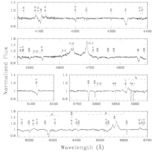
Figure 1: Most important parts of the optical spectrum of LSS 3074 as observed with the EMMI instrument at the NTT on HJD 2 452 355.7, $\phi=0.40$. This spectrum is not corrected for the telluric absorption, and the main telluric bands are shown with dashed lines (Curcio et al. Curcio (1964)).

4 Orbital solution

Since LSS 3074 is a rather faint and heavily reddened object, the accuracy of any radial velocity (RV) determination is mainly limited by the S/N ratio of the data. Therefore, we have concentrated our efforts on the strongest absorption lines that are essentially free from blends with other features. In this way, we have measured the RVs of H$\gamma$, He i $\lambda\lambda$ 4471, 5876, and 7065 and He ii $\lambda\lambda$ 4542, 5412, and 6406 in the spectra. We adopted the effective wavelengths of Underhill (Underhill (1995)), as listed in Table 4.

Table 4: Adopted wavelengths of the lines used to measure the RVs of LSS 3074.

Spectrum	Wavelength (Å)
H i	4340.47
He i	4471.48
He ii	4541.59
He ii	5411.52
He i	5875.62
He ii	6406.44
He i	7065.24

Spectrum	Wavelength (Å)
N iv	4057.80
N v	4603.83
N v	4619.90
N iii	4634.16
N iii	4640.64

For each observation, the RVs of the primary and secondary components were computed as the mean of the corresponding RVs measured for the above listed lines on that observation. Unfortunately, either because of a low S/N or other problems, not all of these lines could be measured on all of our spectra. For instance, while we managed to deblend the primary and secondary components of the He i lines on most of our spectra, the intensity contrast between the two components is much larger for H$\gamma$ and for the He ii lines. Therefore, the secondary component of the latter lines could only be resolved on the spectra with the highest S/N ratio. Another example is He ii $\lambda$ 5412: the proximity of several DIBs of similar strength as the secondary line and the fact that the line develops a P-Cygni type profile (with an emission component at a velocity of $\sim 200$ km s^-1) between phase $\phi=0.35$ and $0.50$ lead to rather complex blends and thus highly uncertain RVs at these specific orbital phases. As a result, not all of the RV data points are based on the same set of lines. Yet, it is well known that in early-type stars featuring relatively strong winds, the systemic velocities of the different spectral lines can be significantly different (Rauw et al. HDE228766 (2002)). Therefore combining different sets of spectral lines for different dates could bias the orbital solution. To circumvent this problem, we tied the RVs of the different lines to a single systemic velocity for each component. To do so, we first noted that the He i $\lambda$ 5876 line is the one for which RVs of both components could be determined on nearly all observations, despite the fact that these absorptions lie on top of a broader emission. We thus selected He i $\lambda$ 5876 as our reference line. The positions of the primary and secondary He i $\lambda$ 5876 lines are shown in Fig. 4. For each of the other lines that we measured, we then determined the mean RV shift compared to He i $\lambda$ 5876, and we subtracted this mean shift from the actual measurements. For each observation, the corrected RVs were then averaged, resulting in a homogeneous set of values, expressed in the rest frame of the He i $\lambda$ 5876 line.

These resulting RVs are listed in Table 1. For most data points, the uncertainties on these RVs are about 10-15 km s^-1. In some cases however (indicated by the colons in Table 1), the uncertainties are larger than 20 km s^-1 and can reach $\sim$40 km s^-1 in one case (HJD 2 452 382.597). To adopt the same notations as previous investigators, we refer to the brightest and hottest component of LSS 3074 as the primary, though its present-day mass appears to be lower than that of its companion (see below).

Owing to the severe aliasing problem, it is extremely difficult to obtain an independent determination of the orbital period of LSS 3074 from our set of RV measurements only. A Fourier analysis of the RV₁ and RV₂ data yields the highest peaks around $\nu=0.46020$ d^-1 ($P{}_{{\rm orb}}=2.1730$ days) and $\nu=0.45762$ d^-1 ($P{}_{{\rm orb}}=2.1852$ days). However, we caution that there are many more aliases that could hide the actual orbital period. It is worth pointing out that the second peak yields almost exactly the same period as found by Niemela et al. (Niemela (1992)). We performed the same Fourier analysis for each of the four bandpasses of the photometric data, $B$, $V$, $R$, and $I$, and obtained a highest peak at $\nu=0.9158$ d^-1, which corresponds to an orbital frequency of $\nu=0.9158/2=0.4579$ d^-1, corresponding to $P{}_{{\rm orb}}=2.184$ days. While the periodogram of the photometric time series allows us to unambiguously identify the correct alias, the natural width of its peaks is much larger than in the case of our spectroscopic time series. In fact, folding the RVs into the photometric period yields an unacceptably large scatter. Therefore, combining the results from periodograms of the photometric and spectroscopic time series, we find that the most likely period of LSS 3074 is 2.1852 $\pm$ 0.0006 days, with the error bars given as 1$\sigma$ deviation.

Also, the $T{}_{0}$ obtained with the photometric curves is HJD 2 452 000.9568, which corresponds to a phase shift of $\sim$0.05 with the $T{}_{0}$ obtained with the RV data. If we lock the RV data to this $T{}_{0}$, we obtain a period of 2.1849 days. Considering that this result is well within the error bars of our previous calculations, we can admit the phase alignment of the RV and photometric data.

As a consistency check, we also combined our measurements in the $V$ band with those taken by Haefner et al. in Haefner (1994) and obtained a highest peak of the periodogram at $\nu=0.9153$ d^-1, which corresponds to an orbital frequency of $\nu=0.9153/2=0.45765$ d^-1, corresponding to $P{}_{{\rm orb}}=2.1851$ days. This result tends to confirm the quality of our determination of the orbital period of the system.

Adopting an orbital period of 2.1852 days, we computed an orbital solution assuming a circular orbit. The RVs were weighted according to their estimated uncertainties. The result is shown in Fig. 2 and the corresponding orbital elements are provided in Table 5.

Table 5: Orbital solution computed from our RV data of LSS 3074 assuming a circular orbit and an orbital period of 2.1852 days.

	Primary	Secondary
$T{}_{0}$ (HJD - 2 450 000)	2000.851 $\pm$ 0.008
$\gamma$ (km s-1)	-66.0 $\pm$ 5.0	-21.7 $\pm$ 4.7
K (km s-1)	228.5 $\pm$ 7.1	196.0 $\pm$ 6.1
a sin i (R⊙)	9.9 $\pm$ 0.3	8.5 $\pm$ 0.3
q = m1/m2	0.86 $\pm$ 0.04
m sin3i (M⊙)	8.0 $\pm$ 0.5	9.3 $\pm$ 0.7
$R{}_{{\rm{RL}}}$/($a{}_{1}+a_{2}$)	0.37 $\pm$ 0.01	0.39 $\pm$ 0.01
$R{}_{{\rm{RL}}}$ sin i (R⊙)	6.7 $\pm$ 0.2	7.2$\pm$ 0.2
$\sigma_{{\rm fit}}$	3.11

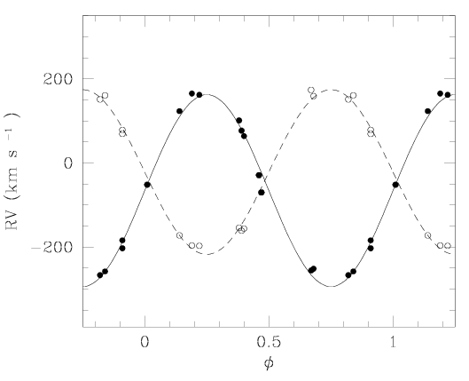
Figure 2: Radial velocities of the components of LSS 3074 assuming a period of 2.1852 days. The RVs of the primary and secondary stars are shown with filled and empty circles, respectively. The solid and dashed lines indicate the orbital solution from Table 5.

The RV amplitudes of our solution are in reasonable agreement with values from the literature ($K{}_{1}=222$ and $K{}_{2}=218$ km s^-1; Niemela et al. Niemela (1992)). Consequently our orbital solution also leads to low minimum masses, similar to those of Niemela et al. ($m$ sin${}^{3}i=9.5$ and 10 M_⊙ for the O4f primary and the secondary, respectively). The apparent systemic velocity of the primary is significantly more negative than that of the secondary. This most likely indicates that the absorption lines of the primary are not entirely formed in the static photosphere, but arise at least partly from an expanding stellar wind.

Figure 3 shows the RVs of the nitrogen emission and absorption lines in the spectrum of LSS 3074. The adopted effective wavelengths of the studied lines are listed in Table 4. All the lines seem to move with the primary, but the scatter of the velocities of the various lines is rather large, especially at phases between the 0.25 quadrature and 0.5 conjunction. During this phase interval, the N iii emission lines yield systematically larger velocities than the N v absorption.

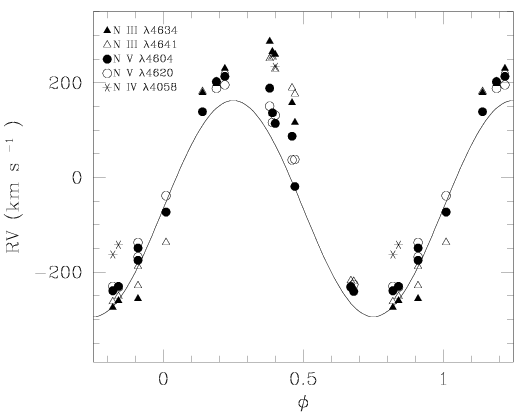
Figure 3: Radial velocities of the N iii and N iv emission lines and the N v absorptions in the spectrum of LSS 3074. The meaning of the various symbols is given in the upper left corner. The solid line yields the orbital solution of the primary from Table 5.

5 Line profile variability

The most prominent emission lines in the optical spectrum of LSS 3074 show strong profile variations (see Fig. 4). For instance, the He ii $\lambda$ 4686 line evolves from a broad and skewed emission (around $\phi=0.0$) into a double-peaked feature with rather narrow individual peaks and the strongest peak closely following the orbital motion of the primary (at phases near 0.5).

On the other hand, the H$\alpha$ emission features a double-peaked profile on most of our spectra and the profiles observed around the two conjunctions are very similar. At phases near quadrature, the peaks are broader and less clear cut. Apart from the moving absorption lines, the He i $\lambda$ 5876 profile has a morphology relatively similar to that of the H$\alpha$ line.

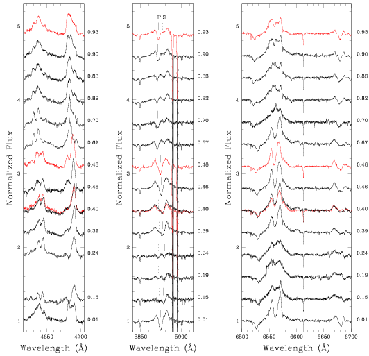
Figure 4: Line profile variations of some important emission lines in the optical spectrum of LSS 3074. N iii $\lambda\lambda$ 4634-4641 and He ii $\lambda$ 4686 are shown in the left panel; He i $\lambda$ 5876 is represented in the central panel; and H$\alpha$ is indicated in the right panel. The orbital phases computed according to the ephemerides in Table 4 are given on the right of each panel. The red spectra correspond to the EMMI observations. The vertical solid (resp. dotted) lines in the middle panel represent the position of the primary (resp. secondary) He i $\lambda$ 5876 line for the given observation.

We measured the equivalent widths (EWs) of the H$\alpha$ line between 6513 and 6604 Å. We find that $\overline{{\rm EW}}=4.09\pm 0.60$ Å. Although the dispersion around the mean is quite large, no obvious phase-locked behaviour is apparent. In particular, we do not see any variations attributable to the modulation of the continuum.

These complex line morphologies make it impossible to assign a single RV to the He ii $\lambda$ 4686 and H$\alpha$ emission lines, and suggest that these lines do not arise in the atmosphere of one of the two stars, but stem from an extended emission region. To further quantify this situation, we used the method of Doppler tomography to map the emitting regions of the He ii $\lambda$ 4686 and H$\alpha$ lines in velocity space. Our method is based on the Fourier-filtered back projection technique (Horne Horne91 (1991), Rauw et al. HDE228766 (2002), Mahy Mahy11 (2011)). The radial velocity of any gas flow that is stationary in the rotating frame of reference of the binary can be expressed as

$$v(\phi)=v_{x}\,\cos{(2\,\pi\,\phi)}-v_{y}\,\sin{(2\,\pi\,\phi)}+v_{z}$$ (5)

where $\phi$ stands for the orbital phase with $\phi=0.0$, corresponding to the primary star being in front. The $(v_{x},v_{y},v_{z})$ are the velocity coordinates of the gas flow. The $x$ and $y$ axes are located in the orbital plane. The $x$-axis runs from the primary to the secondary, whilst the positive $y$-axis points in the direction of the orbital motion of the secondary. The $v_{z}$ component represents the apparent systemic velocity of the line under consideration. The Doppler map consists of a projection of relation given by (5) on the $(v_{x},v_{y})$ plane. For a given value of $v_{z}$, each pixel in a Doppler map, specified by its velocity coordinates, is therefore associated with a particular form of equation (5). All our spectra listed in Table 1 were given equal weights. The Doppler maps, computed adopting $v_{z}=-44$ km s^-1, are shown in Fig. 5. They reveal extended line formation regions in velocity space with different morphologies for the two lines. The He ii $\lambda$ 4686 line features an emission lobe on the negative $v_{x}$ side and mostly with negative $v_{y}$. This emission seems thus mostly associated with the primary star. The H$\alpha$ Doppler map displays two lobes, extending on both sides of the Roche lobes in velocity space, with the strongest one closely matching the emission lobe of the Doppler map of He ii $\lambda$ 4686.

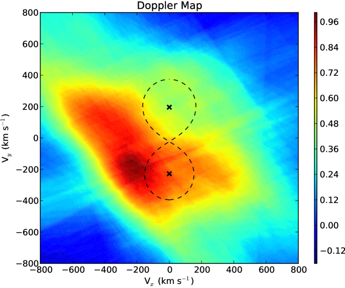
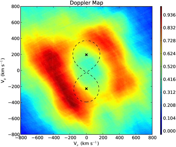
Figure 5: Doppler maps of the He ii $\lambda$ 4686 (left) and H$\alpha$ (right) emission lines in the spectrum of LSS 3074. The crosses correspond to the radial velocity amplitudes of the centre of mass of the primary (negative $v{}_{y}$) and secondary (positive $v_{y}$), whereas the dashed lines indicate the Roche lobe in velocity space for a mass ratio $m_{1}/m_{2}=0.86$. The colour scale indicates the level of the line emissivity relative to its maximum value.

A full interpretation of these Doppler maps in terms of wind-wind interactions is beyond the scope of the present paper. However, it is interesting to compare our Doppler maps with those of Algol-type systems where a cool star fills up its Roche lobe and transfers matter to a hotter companion (Richards et al. Richards14 (2014)). Our maps are clearly different from those presented by Richards et al. (Richards14 (2014)). The structures seen in Fig. 5 neither resemble those produced by gas streams that directly impact the mass gainer nor do they feature the ring-like structure, centred on the mass gainer, that appears for systems with Keplerian accretion disks. These results therefore do not support the presence of an accretion disk or an accretion stream in LSS 3074.

6 Preparatory analysis

6.1 Spectral disentangling

The determination of the orbital solution allowed us to recover the individual spectra of both components through the disentangling of the normalized spectra of the binary system. For this purpose, we used our disentangling routine (Rauw DSc (2007)) based on the method of González & Levato (GL (2006)), previously used by Linder et al. (Linder (2008)) and improved by Mahy et al. (Mahy (2012)). In this procedure, the mean spectra of each binary component are reconstructed in an iterative way by shifting the observed data into the frame of reference of one star and subtracting the best approximation of the spectrum of the other star shifted to its observed radial velocity. In the disentangling carried out in this work, we fixed the RVs of the binary components to those corresponding to the orbital solution of Sect. 4. For a more detailed description of the method, see Raucq et al. (Raucq (2016)).

As for any disentangling method, this technique also has its limitations (González & Levato GL (2006)). An important limitation for our study is that broad spectral features are not recovered with the same accuracy as narrow ones. Indeed, features that are wider than a few times the RV amplitude are barely properly recovered. This is the case of the wings of the Balmer lines, for example. Moreover small residual errors in the normalization of the input spectra can lead to oscillations of the continuum in the resulting disentangled spectra on wavelength scales of several dozen Å, and a reasonable observational sampling of the orbital cycle is needed because the quality of the results depends on the radial velocity ranges covered by the observations. Finally, spectral disentangling works on continuum-normalized spectra and does not yield the brightness ratio of the stars, which must be determined by other techniques (see below).

In the particular case of LSS 3074, we also encountered problems due to the large brightness ratio of the system. Indeed, as shown in Sect. 6.3, the primary star appears much brighter than the secondary star, meaning that the latter is faint in the observed spectra, which induces difficulties in the disentangling procedure, a lower S/N ratio, and thus larger uncertainties on the resulting secondary spectrum.

6.2 Spectral types

We then determined the spectral types of the stars through the measurement of the equivalent width ratio of some spectral lines of the reconstructed individual line spectra of the primary and secondary components. We used the He i $\lambda$ 4471 and He ii $\lambda$ 4542 lines, on the one hand, and Si iv $\lambda$ 4089 and He i $\lambda$ 4143 lines, on the other hand, and applied the Conti quantitative classification criteria for O-type stars (Conti & Alschuler CA (1971), Conti & Frost CF (1977), see also van der Hucht vdHucht (1996)) for both spectral types and luminosity classes. In this way, we obtain O5.5 I and O6.5-7 I classifications for the primary and secondary, respectively. The strong He ii $\lambda$ 4686 and N iii $\lambda\lambda$ 4634-41 emission lines lead to the addition of an f qualifier (see Walborn et al. Walborn02 (2002), Sota et al. Sota11 (2011), Maíz Apellániz et al. Jesus (2016) and references therein) for both components. The primary spectrum further displays emissions of Si iv $\lambda\lambda$ 4089, 4116. Previously these features were indicated by an f⁺ qualifier, but it has been suggested that this notation is obsolete (Sota et al. Sota11 (2011)).

However, the Conti criterion for the luminosity classes is formulated for spectral types from O7 to O9.7 and its application to the spectrum of the primary star is thus an approximation. Moreover, Walborn et al. (Walborn02 (2002)) argued that it would be preferable to use the N iv/N iii emission line ratio for the spectral classification of the earliest O-type stars rather than the ratio of the He i/He ii absorption lines. As shown in Fig. 3, the N iii $\lambda\lambda$ 4634, 4641, and the very weak N iv $\lambda$ 4058 emission line (when present) clearly move along with the primary star. The same holds true for the weak, but definite N v $\lambda\lambda$ 4604 and 4620 absorption lines. As indicated in Sect. 3, the presence of these N v absorption lines points towards a rather hot star with an O3 to O4 spectral type (Walborn et al. Walborn02 (2002), Sota et al. Sota11 (2011)), which is at odds with our above classification based on the helium lines. We have thus compared our disentangled primary spectrum with the spectral atlas of Sota et al. (Sota11 (2011)). The strong He ii $\lambda$ 4686 emission clearly confirms a supergiant luminosity class. The simultaneous presence of strong N iii, very weak N iv, and definite N v lines in the spectrum of the primary is clearly a challenge both for spectral classification and spectral modelling (see Sect. 8.4). The best match, although certainly not perfect, is found with the spectra of HD 14 947 (O4.5 If) and, to a lesser extent, HD 15 570 (O4 If). For a highly deformed star, such as the primary of LSS 3074, gravity darkening leads to a non-uniform surface temperature. Hence, the discrepancy between the O5.5 If spectral type inferred from the relative strengths of the He i and He ii lines and the O4-4.5 If type derived from the nitrogen spectrum could simply reflect the fact that these lines form over different parts of the stellar surface. We come back to this point in Sect. 8.4. For the secondary star, comparison with the atlas of Sota el al. (Sota11 (2011)) yields a spectral classification O6.5-7 If, in agreement with the results from the relative strengths of the helium lines.

Finally, since our classification is based on the disentangled spectra, it is less sensitive to a possible phase dependence of the line strengths and should thus be more robust than a classification based only on spectra collected near quadrature phases.

6.3 Brightness ratio

The spectral disentangling yields the strength of the lines in the primary and secondary stars relative to the combined continuum. But as we mentioned earlier, it does not allow us to establish the relative strengths of the continua. We therefore needed to first establish the brightness ratio of the stars to further analyse the reconstructed spectra.

To estimate the optical brightness ratio of the components of LSS 3074, we measured the equivalent widths, referring to the combined continuum of the two stars, of a number of spectral lines on the reconstructed primary and secondary spectra. The results are listed in Table 6 along with the mean equivalent widths of the same lines in synthetic spectra of stars of the same spectral type, computed with the non-LTE model atmosphere code CMFGEN (Hillier & Miller HM (1998)), which we describe in Sect. 8.2. For comparison, we also list the mean equivalent widths of the same lines in spectra of stars of similar spectral type as measured by Conti (Conti1 (1973, 1974)) and Conti & Alschuler (CA (1971)).

Table 6: Brightness ratio determination from the dilution of prominent lines.

Line	Equivalent Width (Å)						$l{}_{1}/l_{2}$
	Observations		Synthetic spectra		Conti (Conti1 (1973, 1974))
	Primary	Secondary	O5.5	O7	O5.5	O7
He i $\lambda$ 4026	0.42	0.19	0.51	0.69	0.46	0.61	3.00
He ii $\lambda$ 4200	0.41	0.17	0.53	0.45	0.58	0.59	2.00
H$\gamma$	0.90	0.34	1.56	1.75	1.85	2.22	3.00
He i $\lambda$ 4471	0.25	0.26	0.29	0.61	0.29	0.59	2.08
He ii $\lambda$ 4542	0.56	0.19	0.62	0.53	0.75	0.67	2.43

The brightness ratio of the two stars can then be evaluated from

$\frac{l_{1}}{l_{2}}=(\frac{EW_{1}}{EW_{2}})_{{\rm obs}}(\frac{EW_{O7}}{EW_{O5.5}})_{{\rm mean}}$.

By combining our measurements with those from synthetic spectra, we derive an optical brightness ratio of $2.50\pm 0.43$. As a consistency check, we can also determine the brightness ratio through a comparison with the measurements made by Conti, and we obtain $2.61\pm 0.41$.

The disentangled continuum normalized primary and secondary optical spectra are shown in Fig. 8.

7 Light curve

To improve our understanding of the system LSS 3074, and in particular its geometry, we performed an analysis of the photometric light curves by modelling the system using the eclipsing binary star simulator NIGHTFALL, developed by Wichmann, Kuster and Risse. We worked in an iterative way. First of all, we fixed the mass ratio and orbital period to the values obtained from the orbital solution (see Table 5) and the effective temperatures to typical values for stars of similar spectral types (Martins et al. Martins2 (2005)). This permitted us to obtain a first estimation of the photometric solution and of the stellar radii and masses. Based on these approximated parameters, together with the effective temperatures, we calculated the associated surface gravities and stellar luminosities. This first approximation of the stellar fundamental parameters was then used as starting point input in our study of the atmosphere modelling procedure (see Sect. 8.2 and 8.3). This procedure then permitted us to accurately determine the effective temperatures of the stars, giving us a new input for the light curve study with NIGHTFALL.

Inspection of the light curve reveals a lack of a plateau between the minima, indicating important contributions of ellipsoidal variations to the photometric variability. Actually, the shape of the light curve suggests that almost the entire photometric variations could stem from such ellipsoidal variations, thereby implying that at least one of the stars must fill or overflow its Roche lobe.

The only evidence for the existence of genuine eclipses comes from the fact that the secondary minimum seems about 0.02 mag deeper than the primary minimum. The primary minimum corresponds to the occultation of the primary star by the secondary. What is surprising here is that the deeper minimum actually corresponds to the spectroscopically hotter star being in front. Given the level of dispersion in the light curve, it is quite possible that the small difference in depth of the minima is not significant and could arise, for example, from intrinsic variations of the stars. An alternative explanation for this situation could be an atmospheric eclipse produced by the wind of the primary star. Antokhina et al. (Antokhina13 (2013)) studied the impact of free electron scattering in the wind of one star on the light curves of close eclipsing binaries. For a contact binary made of otherwise equal stars, these authors show that the presence of a stellar wind with $\dot{M}=10^{-5}$ M_⊙ yr^-1 around one component deepens the eclipse corresponding to the star with the wind passing in front of its companion by about 0.08 mag. At the same time, the depth of the other eclipse is slightly reduced. In the case of LSS 3074, the fact that most emission lines closely follow the motion of the primary star suggests that this star has the strongest wind, thus lending support to this explanation. However, as pointed out by Antokhina et al. (Antokhina13 (2013)), a quantitative assessment of the impact on the light curve requires some independent determination of the wind parameters (mass-loss rate, asymptotic velocity and exponent of velocity law). In our case, this is difficult to achieve (see Sect. 8). This is because of the lack of UV spectroscopy and the complexity of the line emission regions. Indeed, as revealed by our tomographic analysis, at least parts of the H$\alpha$ and He ii $\lambda$ 4686 emissions arise from an interaction zone and these lines hence do not necessarily reflect the genuine properties of the winds. Yet, our best-fit model atmosphere parameters (see the forthcoming Table 10) yield upper limits on the wind density that could be consistent with the observed difference in eclipse depth. However, these best-fit parameters also suggest that both binary components lose material at a similar rate. Hence, one would expect both eclipses to be affected by stellar wind absorption. We thus conclude that a better knowledge of the wind parameters of LSS 3074 is required before we can attempt a model of the light curve accounting for the effects of the stellar winds. Whatever the origin of the slight difference in depth of the minima, we need to keep in mind that this situation affects the quality of the fits of the light curve.

To explain the shape of the secondary minimum by the sole effect of ellipsoidal variations, we at least need to assume that either both components of the binary system fill up (contact-contact) or even overflow their Roche lobes (overcontact), or that one of the components must be much smaller and much fainter than the other star that fills up its Roche lobe. In the former case, one expects both stars to be of very comparable size and, given their effective temperatures, also of rather comparable brightness. To explain the depth of almost 0.2 mag by the sole effect of ellipsoidal variations is actually not possible here without requiring the presence of true eclipses. In this context, the necessity to invoke a contact-contact or an overcontact configuration remains valid, along with the conclusion that sizes and brightness of both stars should be comparable.

This is precisely the outcome of our fits with the NIGHTFALL code. The best-fit quality ($\chi^{2}_{\nu}=4.4$) is achieved for overcontact configurations with a filling factor of 1.008 ($i\simeq 54.5^{\circ}$), where the corresponding $V$-band brightness ratio is predicted to be 1.09. The corresponding photometric solution is presented in Table 9 and the associated plot is shown in Fig. 6. Yet, our spectroscopic analysis suggests an optical brightness ratio (primary/secondary) near 2.50. This situation is thus clearly at odds with explaining the photometric light curve via a double contact or overcontact configuration. To achieve a brightness ratio of $2.50\pm 0.43$, the ratio between the mean radii of the primary and secondary stars would have to be $1.15\pm 0.10$. This translates into a ratio of the filling factors of $1.23\pm 0.11$, which is only possible for detached or semi-detached configurations. As could be expected, the fact that the hotter star is in front during the deepest minimum leads to difficulties to fit this minimum.

Since the eclipses are only partial, one way to solve this issue would be to postulate the existence of a dark spot on the side of the secondary star facing the primary. Such a spot would then lead to a deeper minimum when the primary star is in front. From a purely numerical point of view this would improve the fit quality significantly with $\chi^{2}_{\nu}$ now approaching 2.9. In addition, it would certainly help to bring the spectroscopic and photometric brightness ratios into better agreement. Yet, aside from the difficulty of explaining the physical origin of such a spot, there is another issue that concerns the fact that the spot size and its dim factor (i.e. the reduction in local temperature) are not fully independent and we lack any objective constraints on these parameters. Test calculations have shown that for some situations, the best-fit model would actually correspond to a spot that covers more than 75 $\%$ of the surface of the secondary, which is clearly not physical.

Table 7: Photometric solution for LSS3074.

Parameters	Primary	Secondary
i (°)	$54.5\pm 1.0$
q = m1/m2

0.86 (fixed)    Filling factor & $1.008\pm 0.010$ $1.008\pm 0.010$ $T_{\rm eff}$ (K) 39 900 (fixed) 34 100 (fixed) $m$ (M_⊙) $14.8\pm 1.1$ $17.2\pm 1.4$ $R_{\rm pole}$ (R_⊙) 7.8 8.4 $\chi^{2}$    1820.7    $N_{{\normalcolor{\rm{dof}}}}$    415

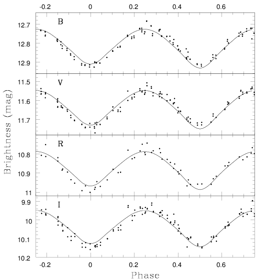
Figure 6: Photometry of LSS 3074. The observational data are presented as black dots, and the solid black line corresponds to the best-fit theoretical light curve fit with NIGHTFALL with the parameters presented in Table 9. The zero phase corresponds to the secondary eclipse, when the primary is occulting the secondary.

As an alternative to the overcontact configuration, one might consider a scenario where the primary star overflows its Roche lobe and transfers matter to a geometrically thick accretion disk around the more massive secondary star. This kind of scenario has been proposed to explain the light curves of $\beta$ Lyrae (Wilson Wilson (1974)), RY Sct (Antokhina & Kumsiashvili RYSct (1999)), and V455 Cyg (Djurašević et al. V455Cyg (2012)), among others. On the positive side of such a scenario, it might help reconcile the photometric and spectroscopic brightness ratios. On the negative side, we have the lack of a clear signature of an accretion disk in the Doppler maps of the H$\alpha$ line and the fact that LSS 3074 is a very compact system, leaving very little room for the formation of a disk, unless the secondary star is very small. To test this scenario, we used the disk option in the NIGHTFALL code. In addition to the effective temperatures that we fixed at the values obtained from our model atmosphere fits (see Sect. 8.3), we set the Roche lobe filling factor of the primary star to unity and that of the secondary star to 0.75. This choice results in a brightness ratio that is consistent with our spectroscopic value. We tested various options for the disk available in the NIGHTFALL code (simple disk with uniform temperature, isothermal disk and reprocessing disk), which correspond to different prescriptions of the variations of the disk height and temperature with radius. Since the disk in our models resembles more an annulus than a genuine disk, these three options actually yield nearly identical results. These models fail to reproduce the width of the secondary minimum. This failure increases the $\chi^{2}$ of the fits. Still, we managed to find fits with $\chi_{\nu}^{2}\sim 4.6$, but this was only possible for a disk temperature exceeding the temperatures of both stars, which is most probably not physical. Better quality fits can be obtained if the Roche lobe filling factor of the secondary is allowed to drop below 0.75: we obtained $\chi_{\nu}^{2}=3.9$ for a secondary filling factor of 0.47 (which would correspond to a secondary radius of only 3.9 R_⊙) and a disk temperature of 51 300 K. Both parameters (secondary radius and disk temperature) are most probably not physical. We thus conclude that a disk model cannot solve the issues raised above any better than the pure Roche potential model.

From a purely phenomenological point of view, we can expand the light curve into a sum of sine functions. We tried a period of 2.1852/2 = 1.0926 days and a mere sine and a period of 2.1852 days and the fundamental sine plus its harmonic. The results are given in Table 8. The photometric observations exhibit a variation with a semi-amplitude of 0.09 mag in all filters. The semi-amplitude associated with the modulation on the orbital period is 0.01 mag reflecting the above-mentioned difference between the depths of the two minima. The corresponding $\chi_{\nu}^{2}$ are lower than for any other fit we tried but still not satisfactory. Including a larger number of harmonics in our expansion does not improve the situation. However, in terms of standard binary models, this fit is unphysical since a modulation with a semi-amplitude as large as 0.09 mag cannot be explained by ellipsoidal variations for such models. The fit of the $B$ light curve corresponds to a larger $\chi_{\nu}^{2}$; the corresponding $\chi_{\nu}^{2}$ would be similar to those found for the data from the other filters provided that the photometric errors used to normalize the $\chi_{\nu}^{2}$ were 0.010 mag instead of 0.007 mag.

Table 8: Fit of the light curves of LSS 3074 by a sine function.

	Filter
	$B$	$V$	$R$	$I$
$P=1.0926$ d
$a(P)$	0.0901	0.0910	0.0964	0.0980
$\sigma{}_{a}$	0.0022	0.0022	0.0039	0.0027
$\chi_{\nu}^{2}$	5.96	2.92	2.65	2.66
$\sigma_{{\rm fit}}$	0.0171	0.0171	0.0212	0.0212
$P=2.1852$ d
$a_{1}(P)$	0.0118	0.0125	0.0107	0.0125
$\sigma{}_{a_{1}}$	0.0020	0.0020	0.0038	0.0020
$a_{2}(P/2)$	0.0896	0.0905	0.0958	0.0905
$\sigma{}_{a_{2}}$	0.0019	0.0019	0.0037	0.0019
$\chi_{\nu}^{2}$	4.60	2.20	2.38	1.30
$\sigma_{{\rm fit}}$	0.0150	0.0148	0.0200	0.0148
$N$	120	122	58	118
$\sigma$	0.007	0.010	0.013	0.013

The $\chi_{\nu}^{2}$ of Table 8 are too large and this anomaly could have several origins. One possibility is that the above-mentioned photometric errors deduced from the comparison stars might not apply to the case of LSS 3074. This could be due to an unfortunate location on the CCDs or for example to strange behaviour due to peculiar stellar colours. This interpretation is however not very likely. Alternatively, the fitted mathematical model might not be correct. Since any periodic function can be expanded into a Fourier series and we found that our sine fits do not require additional terms, the additional, non-periodic component of the model behaves similarly to an observational noise although it must have a different origin. A possible explanation could be an intrinsic variability of the star at high frequencies since no low-frequency variations were previously detected beyond the orbital one. Of course, this additional component has an upper limit. Since the sine fits are our best models, we can consider estimating this upper limit from the corresponding residuals. In the $V$ filter for instance, we would need an additional variability compared to the expected $\sigma=0.010$ mag photometric error that quadratically adds to it to reach $\sigma_{{\rm fit}}=0.0148$ mag for the two periods fit or $\sigma_{{\rm fit}}=0.0171$ mag for the single period fit. Considering that the difference in depth between the two minima is not well established, we can adopt the latter and the relevant value would thus be $\sigma_{{\rm fit}}=0.0171$ mag.

The transition from $\sigma=0.010$ to $0.0171$ mag translates into a change from $\sigma=0.009$ to $\sigma^{{\rm corr}}=0.0185$ mag for the global fit of the data from all four filters. The substitution by these newly estimated errors alleviates the rejection of the NIGHTFALL model, since it reduces the $\chi{}^{2}$. However, this is purely artificial. In addition, the $\chi_{\nu}{}^{2}$ of 4.4 could still be due to a lack of ability of the NIGHTFALL model to fit the light curve, even if it were noiseless. However, under the hypothesis of the fit of the NIGHTFALL model, the errors on the parameters must be modified to remain coherent. Even though this additional dispersion does not stem from the same origin as the genuine photometric errors, impact of this dispersion on the derived parameters is similar to that of photometric errors.

To obtain the 1$\sigma$ error on the parameters of the NIGHTFALL models, we have to consider the dispersion at $\chi_{{\rm min}}^{2}+\Delta\chi_{1\sigma}^{2}$ where $\Delta\chi_{1\sigma}^{2}=2.3$ for the 1$\sigma$ confidence interval of the simultaneous adjustment of two free parameters ($i$ and $fill_{{\rm p}}$ = $fill_{{\rm s}}$ as is the case when we fit the light curve assuming an overcontact configuration with NIGHTFALL). From the values of the $\chi^{2}$ of our best-fit NIGHTFALL model, the 1$\sigma$ error bars on the orbital inclination and the filling factors would be unrealistically small (e.g. about $0.1^{\circ}$ for the error on $i$). However, as pointed out above, the dispersion of the photometric data about the best-fit synthetic light curve exceeds the value of our estimated photometric errors, suggesting that there could be an intrinsic photometric variability in addition to the orbital modulation.

Admitting the impact of the additional dispersion, we have to correct the $\Delta\chi_{1\sigma}^{2}=2.3$ to take this effect into account. Therefore, we have to adopt a corrected $\Delta\chi_{1\sigma,{\rm corr}}^{2}=\Delta\chi_{1\sigma}^{2}\times\left(\frac{\sigma^{{\rm corr}}}{\sigma}\right)^{2}=8.9$. We have then estimated the errors on the NIGHTFALL model parameters by accordingly adopting this new corrected value. In this way, rounding the values uppards, we estimate errors of $1.0^{\circ}$ and of 0.01 for the inclination and the filling factors of both stars, respectively.

8 Spectral analysis

8.1 Rotational velocities and macroturbulence

In order to determine the projected rotational velocities ($v\,\sin{i}$) of the stars of the system, we applied a Fourier transform method (Simón-Díaz & Herrero Simon-Diaz (2007), Gray Gray (2008)). For the primary star, we used the profiles of the He i $\lambda$ 4471, He ii $\lambda\lambda$  4200, 4542, 6118, and N iii $\lambda$ 6075 lines of the reconstructed spectrum. We selected these lines as they are rather well isolated in the spectra and should thus be free of blends. Unfortunately, we could not use the same lines for the secondary star because they are particularly deformed. Indeed, the red wing of these lines is steeper than the blue wing. We then used the He ii $\lambda$ 5412 and Si iv $\lambda$ 4089 lines to determine the projected rotational velocity of the secondary star. The results are presented in Table 9. The mean $v\,\sin{i}$ of the primary star is $(110\pm 13)$ km s^-1, while that of the secondary is $(127\pm 6)$ km s^-1. Owing to the small number of lines usable to study the rotation of the secondary star, we could not use a classical standard deviation method to determine the associated error bars. We thus studied the Fourier transforms for a sample of rotational velocities to estimate these errors. From these values of $v\,\sin{i}$ and considering the inclination of the system from Sect. 7, we found that the stars are in synchronous rotation with a rotational period very close to the orbital period of the system.

Table 9: Projected rotational velocities ($v\,\sin{i}$ expressed in km s^-1) of the components of LSS 3074.

Line	Primary	Secondary
Si iv $\lambda$ 4089	-	126
He ii $\lambda$  4200	115	-
He i $\lambda$ 4471	97	-
He ii $\lambda$  4542	119	-
He ii $\lambda$ 5412	-	128
N iii $\lambda$ 6075	92	-
He ii $\lambda$ 6118	125	-
Mean value	110 $\pm$ 13	127 $\pm$ 6

Macroturbulence is defined as a non-thermal motion in the stellar atmosphere with turbulent cells larger than the mean free-path of the photons. The main effect of macroturbulence is an additional broadening of the spectral lines. An approximation of the macroturbulence velocities was obtained by applying the radial-tangential anisotropic macroturbulent broadening formulation of Gray (Gray (2008)) on the spectra, after the inclusion of rotational velocity broadening. For this purpose, we used the auxiliary program MACTURB of the stellar spectral synthesis program SPECTRUM v2.76 developed by Gray (macturb (2010)). We applied this technique to the lines He i $\lambda\lambda$ 4026, 4471, and 5016, and He ii $\lambda$ 4542 and obtained macroturbulence velocities of 20 and 50 km s^-1, for the primary and secondary stars, respectively.

Both rotational and macroturbulence velocities were applied on the synthetic spectra (see Sect. 8.2) before comparing the latter with the disentangled spectra.

8.2 CMFGEN code

In order to determine the fundamental properties of both components of LSS 3074, we used the non-LTE model atmosphere code CMFGEN (Hillier & Miller HM (1998)). This code solves the equations of radiative transfer and statistical equilibrium in the co-moving frame, is designed to work for both plane-parallel and spherical geometries, and can be used to model Wolf-Rayet stars, O stars, luminous blue variables and supernovae. A super-level approach is adopted for the resolution of the equations of statistical equilibrium. The CMFGEN code also further accounts for line blanketing and its impact on the energy distribution. The hydrodynamical structure of the stellar atmosphere is directly specified as an input to the code, and a $\beta$ law is used to describe the velocity law within the stellar winds. We included the following chemical elements and their ions in our calculations : H, He, C, N, O, Ne, Mg, Al, Si, S, Ca, Fe, and Ni. The solution of the equations of statistical equilibrium is used to compute a new photospheric structure, which is then connected to the same $\beta$ wind velocity law. The radiative transfer equations were solved based on the structure of the atmosphere with a microturbulent velocity varying linearly with wind velocity from 20 km s^-1 in the photosphere to $0.1$ × v_∞ at the outer boundary, and generated synthetic spectra were compared to the reconstructed spectra of the primary and secondary stars.

As a first approximation, the mass-loss rates and $\beta$ parameters were taken from Muijres et al. (Muijres (2012)) for the spectral types of both stars, whilst the wind terminal velocity was assumed equal to the mean value for stars of the same spectral type (Prinja et al. Prinja (1990)). We then estimated the surface gravities, stellar masses, radii, and luminosities from our study of the photometric curves. The relevant parameters were then adjusted via an iterative process, as each adjustment of a given parameter leads to some modifications in the value of other parameters. This process and the results we obtained are presented in subsections 8.3 and 8.4, respectively. As explained in Sect. 6, this iterative process was then coupled with a second iterative process, through the study of the photometric light curve.

8.3 Method

The first step is to adjust the effective temperature in the models of the stars. To do so, we adjusted the relative strengths of the He i $\lambda$ 4471 and He ii $\lambda$ 4542 lines (Martins Martins (2011)). Final values are 39 900 and 34 100 K for the primary and secondary stars, respectively. Once the effective temperatures were determined, we used them, together with the stellar radii obtained in our study of the photometric curves, to constrain the luminosities of the stars. We therefore obtained luminosities of $1.38\times 10^{5}L_{\odot}$ and $8.49\times 10^{4}L_{\odot}$ for the primary and secondary stars.

Subsequently, the binarity of the studied system causes some problems. Indeed, the next step is to adjust the surface gravities in the models, but as we mentioned in Sect. 6.1, the wings of the Balmer lines are too broad to be properly recovered by the spectral disentangling. To circumvent this problem, we recombined the models of the primary and secondary star spectra for several phases and compared the resulting binary spectra directly to the observations. This permitted us to better adjust the gravities, but with larger uncertainties than in the case of a single star.

A second problem arises with the adjustment of the wind parameters. Indeed, the He ii $\lambda$ 4686 and Balmer lines may be polluted by some emission from the wind-wind interaction zone. Therefore, the uncertainties on the terminal velocity, the $\beta$ of the velocity law, the clumping factor, the clumping velocity factor, and the mass-loss rate are quite high. Indeed, considering the possible existence of such additional emission polluting these diagnostic lines, the adjustment of the models onto the reconstructed spectra may lead to an underestimate of the terminal velocity, and an overestimate of the $\beta$ of the velocity law, clumping factor, clumping velocity factor, and mass-loss rate. Therefore, the obtained values can only be considered as lower and upper limits of the real properties of the stellar winds. However, we still adjusted them as well as possible: we obtained for the primary and secondary stars values of 2615 and 3055 kms^-1 for $v{}_{\infty}$, 1.30 and 1.40 for $\beta$ and $3.00\times 10^{-6}$ and $3.51\times 10^{-6}$ M_⊙ yr^-1 for the mass-loss rate, based on the strength of H$\alpha$, the width of the He ii $\lambda$ 4686 and H$\alpha$ lines, and both the strengths of H$\gamma$ and H$\delta$, respectively. The clumping formalism used in the CMFGEN model is

$f(r)=f_{1}+(1\text{\textminus}f_{1})e^{(\text{\textminus}\frac{V(r)}{f_{2}})}$

with a clumping filling factor $f_{1}$ of 0.7, a clumping velocity factor $f_{2}$ of 200 kms^-1 and $V(r)$ the velocity of the wind for both primary and secondary stars, and we adjusted these two clumping factors through the strength and shape of H$\alpha$ and H$\beta$ lines.

Finally, once the fundamental properties of the stars had been established or fixed, we investigated the CNO abundances within their atmosphere through the strengths of associated lines. At that point, we encountered several problems. Indeed, there is no visible O line in both primary and secondary spectra, and the only present C lines are the C iv $\lambda\lambda$ 5801 and 5812 lines, which cannot be considered in the determination of the surface C abundance since they can exhibit complex profiles influenced by various phenomena among which is continuum fluorescence (Conti Conti2 (1974); Bouret et al. Bouret (2012)). We thus were only able to determine upper limits for C and O abundances. We used the N iii $\lambda$ 4379 and N iii $\lambda\lambda$ 4511-15-18-24-30-35 lines to adjust the N abundance for the primary star. The same lines were used for the secondary star except for the N iii $\lambda$ 4530 and N iii $\lambda$ 4535 lines. These N abundance diagnostic lines are taken from Martins et al. (Martins3 (2015)) study of a sample of 74 objects comprising all luminosity classes and spectral types from O4 to O9.7. We selected, from their study, all the suggested lines that were significantly seen in our observations. We performed a normalized $\chi^{2}$ analysis to determine the best fit to these lines (Martins et al. Martins3 (2015)). The normalization consists in dividing the $\chi^{2}$ by its value at minimum, $\chi\text{\texttwosuperior}{}_{{\rm}{min}}$. As a 1$\sigma$ uncertainty on the abundances, we then considered abundances up to a $\chi^{2}$ of 2.0, i.e. an approximation for 1 over $\chi\text{\texttwosuperior}{}_{{\rm{min}}}$, as suggested by Martins et al. (Martins3 (2015)).

8.4 Results

Figure 8 shows the best fit of the optical spectra of the primary and secondary stars obtained with CMFGEN, and we present in Table 10 the associated stellar parameters.

Figure 8 reveals that we encountered a lot of difficulty adjusting the spectra of the components of LSS 3074. First of all, it clearly shows that the noise is strongly enhanced in the reconstructed secondary spectrum, because of the high brightness ratio of the system. This peculiarity makes the adjustment of the secondary spectrum even more difficult. Second, if we can see that the He lines are generally well reproduced for both stars, some of these lines in the observed spectra, especially for the secondary star, feature some emission in their wings that is not reproduced by the models. We can also see that the Balmer and He ii $\lambda$ 4686 lines are not perfectly well recovered, probably owing to the complexity of the winds and the presence of a wind-wind interaction zone, as discussed in Sect. 8.3.

Concerning the N lines, most N iii features are reasonably well reproduced by the models, but a few lines of other nitrogen ions are not, especially in the primary spectrum. Indeed, the model predicts a rather strong N iv $\lambda$ 4058 emission, while the observations clearly show that this is not the case. Another remarkable issue is the presence in the observed primary spectra of the N v $\lambda\lambda$ 4604, 4620 lines, which are not predicted by the model. These N v lines are seen in the spectra of the earliest O supergiants (starting from O4 If Walborn et al. Walborn02 (2002), Sota et al. Sota11 (2011)) and, in some cases, in the spectra of early O main-sequence stars (e.g. Mahy et al. Mahy (2012)), and could suggest that our value of the primary effective temperature (39 900 K) is too low. To test this hypothesis, we computed a set of CMFGEN models with temperatures ranging from 38 000 to 44 000 K. As one can see on Fig. 7, a temperature of about 44 000 K would be needed to reproduce the strength of the N v lines. However, in this case, the model predicts N iii emissions that are much weaker than observed as well as a huge N iv line that is clearly not observed. To reproduce the strength of the observed N iii and N iv lines, a lower temperature of 38 000 K seems more indicative. But this lower temperature is clearly not sufficient to produce the N v lines. The temperature that we determined in our CMFGEN fits is the temperature that properly reproduces the strength of the helium lines and represents a compromise between the contradicting trends of the nitrogen lines.

Figure 7: Evolution of the strength of the N iii $\lambda\lambda$ 4634-41, N iv $\lambda$ 4058, and N v $\lambda\lambda$ 4604, 4620 lines in synthetic CMFGEN spectra as a function of effective temperature. The primary spectrum of LSS 3074 obtained via disentangling is shown at the bottom for comparison.

Our difficulty in reproducing simultaneously the lines of N iii, N iv, and N v in the spectra of O supergiants is actually not new. Crowther et al. (Crowther (2002)) and Rauw et al. (HDE228766 (2002)) encountered similar problems in their attempts to fit the spectra of the O4 Iaf⁺ star HDE 269 698 and of the O7 + O4 If/WN8ha binary HDE 228 766, respectively. More recently, Bouret et al. (Bouret (2012)) applied the CMFGEN code to a sample of early O supergiants. These authors also failed to reproduce consistently the lines of the three nitrogen ions in the spectra of the three O4 If supergiants HD 15 570, HD 16 691, and HD 190 429A for which they derived effective temperatures of 38 000, 41 000, and 39 000 K, respectively. We note that these effective temperatures are very close to our best-fit value for the primary of LSS 3074.

The origin of these difficulties is currently unclear. One possibility could be that the models do not account (correctly) for the Auger effect. X-ray emission arising in the wind and back illuminating the stellar photosphere could lead to an overionization of nitrogen and favour the formation of the N v lines. In the specific case of the primary of LSS 3074, the simultaneous presence of the three ionization stages of nitrogen could also be from a non-uniform surface temperature as a result of gravity darkening. Applying the von Zeipel theorem to the primary, we find that the effective temperature near the poles should be about 15% higher than near the equator. The observed spectrum of the primary results from the combination of the spectra emitted by the various regions, which have their own temperatures (Palate & Rauw Palate12 (2012), Palate et al. Palate13 (2013)). Therefore, gravity darkening could indeed result in a spectrum with an unusual combination of spectral lines.

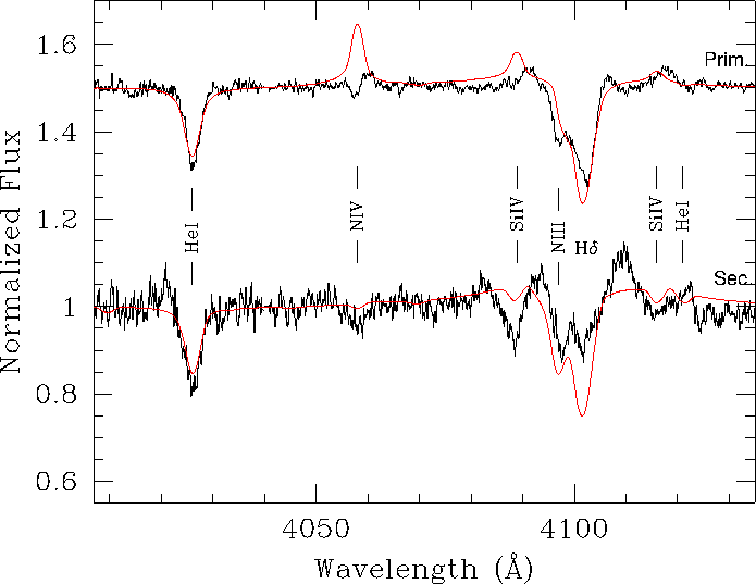
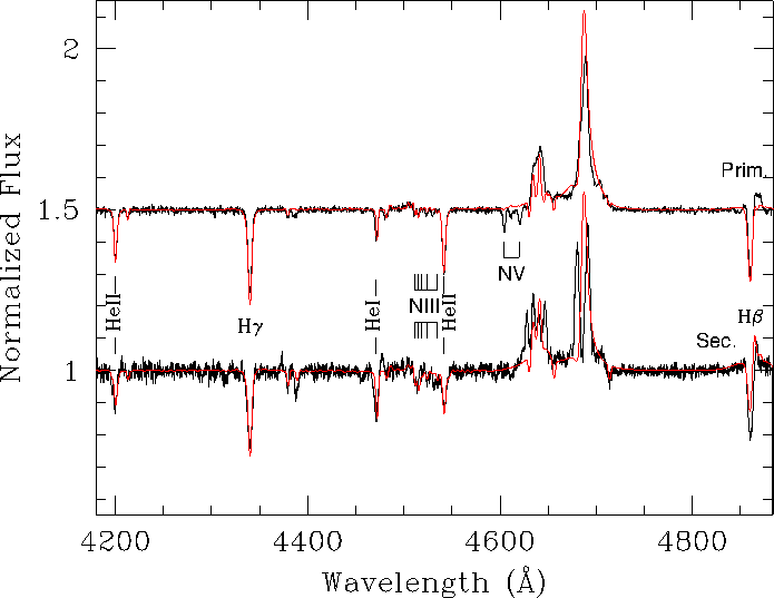
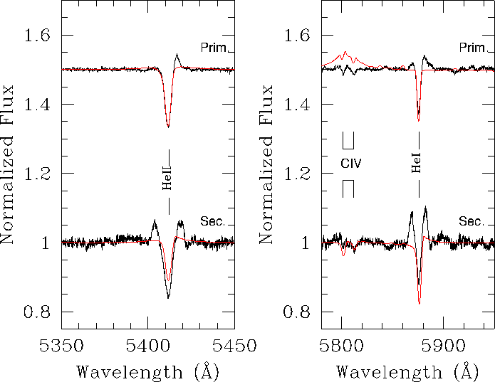
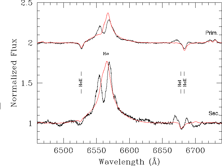
Figure 8: Part of the normalized separated spectra of the primary (top, shifted upwards by 0.5 continuum units in the first three panels, and by 1.0 continuum units for the last panel) and secondary stars (bottom), along with the best-fit CMFGEN model spectra (red).

Table 10: Best-fit CMFGEN model parameters of the primary and secondary stars.

	Prim.	Sec.
$R$ (R⊙)	$7.5\pm 0.6$	$8.2\pm 0.7$
$M$ (M⊙)	$14.6\pm 2.1$	$17.2\pm 3.0$
$T_{{\rm eff}}$ ($10^{4}$ K)	$3.99\pm 0.15$	$3.41\pm 0.15$
log(g) (cgs)	$3.82\pm 0.20$	$3.83\pm 0.20$
log ($\frac{L}{L_{\odot}}$)	$5.14\pm 0.07$	$4.93\pm 0.08$
$\beta$	$\leq$1.30	$\leq$1.40
$v_{\infty}$ (km s-1)	$\geq$2615	$\geq$3055
$\dot{M}/\sqrt{f_{1}}$ (M⊙ yr-1)	$\leq$$3.00\times 10^{-6}$	$\leq$$3.51\times 10^{-6}$

Table 11: Chemical abundances of the components of LSS 3074.

	Primary	Secondary	Sun
He/H	0.25	0.09	0.089
C/H	$\leq 6.45\times 10^{-5}$	$\leq 2.05\times 10^{-5}$	$2.69\times 10^{-4}$
N/H	$5.65{}_{-3.02}^{+4.07}\times 10^{-4}$	$3.69_{-0.91}^{+0.83}\times 10^{-4}$	$6.76\times 10^{-5}$
O/H	$\leq 2.67\times 10^{-5}$	$\leq 1.00\times 10^{-5}$	$4.90\times 10^{-4}$

However, we can stress three very interesting results from our spectral analysis. First of all, as we can see in Table 10, we confirm the very low masses and radii predicted by Morrell & Niemela (Morrell (1990)), which is unusual for stars with such spectral types. We can also see that the system seems to display strong winds, even though these winds are not perfectly constrained. Finally, we found a strong overabundance in N and a strong depletion in C and O in both stars of the system, together with a strong He enrichment of the primary atmosphere.

9 Discussion and conclusions

Our analysis of the light curve of LSS 3074 indicates that this system is a candidate for an overcontact binary. Massive overcontact binaries are important objects as they could be progenitors of merger events or of binary black hole systems (Lorenzo et al. MYCam (2014), Almeida et al. Almeida (2015)). Yet, only a handful of such systems are known and sometimes the exact configuration (double contact versus semi-detached) is controversial (e.g. Yaşarsoy & Yakut V382Cyg (2013) and Zhao et al. LYAur (2014), respectively). Among the best-studied systems hosting O-type stars are HD 100 213 (= TU Mus, Linder et al. Linder07 (2007)), VFTS 352 (Almeida et al. Almeida (2015)), and MY Cam (= BD+56°864, Lorenzo et al. MYCam (2014)). Lorenzo et al. (MYCam (2014)) and Almeida et al. (Almeida (2015)) note that the components of MY Cam and VFTS 352 appear hotter than one would expect from their masses. This discrepancy also exists for LSS 3074 and is even worse than in the other systems. Lorenzo et al. (MYCam (2014)) interpret this result as a consequence of the highly elongated shape of the stars. In the case of VFTS 352, Almeida et al. (Almeida (2015)) further report an enhanced He abundance. These authors interpret this situation as the result of enhanced mixing in a tidally locked binary (de Mink et al. deMink (2009)) and suggest that the system is currently in a long-lived overcontact phase of case A mass transfer. Again LSS 3074 also shows abundance anomalies indicating that both stars are evolved (enhanced N abundance) and the primary is the more evolved star (enhanced He abundance).

9.1 Evolutionary status

We first remark that we did not consider the possibility of quasi-chemically homogeneous evolution as described in Heger et al. (Heger (2000)), because the observed rotational velocities of both components are too small.

The altered CNO abundances in the atmosphere of the primary, the luminosity of primary, and the increased helium abundance are strong arguments that the star is in the slow phase of case B RLOF. If the star were post-RLOF, accounting for the present mass, its luminosity would have to be log ($\frac{L}{L_{\odot}}$) = 5.5 rather than the observed 5.14 (e.g. Vanbeveren et al. VDLVR (1998), formula 5.4). Moreover, the observed CNO abundances of the secondary seem to indicate that at least some mass lost by the primary was accreted by the secondary. The normal (solar) helium abundance, on the other hand, lead us to conclude that not all the helium enhanced layers lost by the primary were accreted by the secondary. Accounting for these facts a theoretical study can be undertaken to attempt to identify its possible progenitors. For this purpose, the Brussels binary population synthesis code is used. This code uses as input thousands of detailed evolutionary calculations performed with the Brussels binary evolution code. Both codes are described in detail in De Donder & Vanbeveren (DeDonder (2004)). However, the theoretical treatment of binary evolution is still subject to a number of uncertainties, which are typically implemented by means of parameters. For the present discussion, two uncertain aspects of binary mass transfer, characterized in population synthesis by two parameters, are of interest. The first is the fraction of the mass lost by the donor star that is actually accreted by the gainer star. This fraction necessarily lies between zero (i.e. totally non-conservative mass transfer) and one (i.e. totally conservative mass transfer), and is characterized in population synthesis by the parameter $\beta_{{\rm RLOF}}$ (hence $0\leq\beta_{{\rm RLOF}}\leq 1$). If $\beta_{{\rm RLOF}}<1$, and thus mass is lost from the system, a second critical assumption concerns how much angular momentum is taken along from the system by this lost mass. This is determined by a parameter $\eta$ (for a formal definition, see De Donder & Vanbeveren DeDonder (2004)). For the present discussion, it suffices to know that the larger $\eta$, the more angular momentum is removed from the binary by a given amount of mass loss. A common assumption made in many population synthesis studies is that the mass lost takes along only the specific orbital angular momentum of the gainer star (and thus leaves this star in a spherically symmetric way). This results in a low angular momentum loss, characterized by a low value of $\eta\sim 0.05$. An alternative assumption is that mass is lost through the second Lagrangian point and forms a circumbinary ring, taking along some of the orbital angular momentum of this ring. This entails a much larger angular momentum loss, and has been shown to result in $\eta=2.3$. Various other, less common assumptions are also possible (e.g. gainer orbital plus spin angular momentum and specific binary angular momentum), which all result in intermediate cases and can be approximated by taking $\eta=1$. The purpose of this paragraph is to investigate, for various combinations of the parameters $\beta_{{\rm RLOF}}$ and $\eta$, whether they can indeed result in the formation of a binary in the slow phase of case B RLOF with the physical parameters (masses and orbital period) of LSS3074, and if so, originating from which initial conditions. All calculations are performed for Solar-like metallicity.

Table 12 shows the initial masses and orbital period, depending on the assumed values of $\beta_{{\rm RLOF}}$ and $\eta$, which produce a 14.8+17.2 M_⊙ binary in the slow phase of case B RLOF and with an orbital period of 2.2 days.

Table 12: Initial masses and orbital period, leading to a 14.8+17.2 M_⊙, 2.2 d post-RLOF binary for different combinations of $\beta_{\rm{RLOF}}$ and $\eta$.

	$\beta_{\rm{RLOF}}=1$	$\beta_{\rm{RLOF}}=0.5$	$\beta_{\rm{RLOF}}=0.1$
$\eta=2.3$	no solution	34+7.9 M⊙, 560 d	34+15 M⊙, 1000 d
$\eta=1$	no solution	34+7.9 M⊙, 90 d	34+15 M⊙, 80 d
$\eta\sim 0.05$	no solution	34+7.9 M⊙, 5.3 d	34+15 M⊙, 1.4 d

Our simulations reveal that the primary progenitor was a star with initial mass 30-35 M_⊙. We find no physically realistic solution if the RLOF is treated conservatively. If it is assumed that $\beta_{\rm{RLOF}}=0.5$, we have to start with an initial 34+7.9 M_⊙ binary. It is however doubtful that a binary with such an extreme initial mass ratio would avoid merging. Our best guess is then a model with $\beta_{\rm{RLOF}}<0.5$, such as the $\beta_{\rm{RLOF}}=0.1$ model of Table 12. If the matter that leaves the binary takes with it the specific angular momentum of the gainer ($\eta=0.05$), the initial period of the binary had to be very small (of the order of 1 or 2 days) and this means that the progenitor binary first went through a case A RLOF phase followed by case B. Interestingly, our simulations show that the slow case B RLOF will stop after some 10000 yrs. The primary star then will be a 11-12 M_⊙ WR star, i.e. the binary will be very similar to the WR binary CQ Cep.

9.2 Summary and conclusions

From what we have seen above, LSS 3074 is clearly a very peculiar binary system that challenges our current methods of binary spectral analysis. In this paper, we have tried to get a deeper understanding of this system, but we encountered a number of problems that prevent us from establishing a fully consistent explanation of all the properties of the system. Here we discuss these problems and try to highlight some avenues for possible solutions.

The properties of the components of LSS 3074 that we determined from our spectral and photometric analysis do not concur with those of genuine early O-type supergiants as determined, for instance, by Bouret et al. (Bouret (2012)). Indeed, these latter authors used the CMFGEN code to analyse UV and optical spectra of typical early and mid-O supergiants. They found that O4-4.5 supergiants have radii between 18.5 and 21.6 R_⊙, $\log{g}$ in the range 3.51 to 3.66 and $\log{L/L_{\odot}}$ between 5.83 and 5.96. For O6-7.5 supergiants, Bouret et al. (Bouret (2012)) determined radii between 20.5 and 21.3 R_⊙, $\log{g}$ between 3.41 and 3.54, and $\log{L/L_{\odot}}$ in the range 5.68 to 5.80. The components of LSS 3074 have significantly smaller radii, which are actually even smaller than the typical radii of early-O main-sequence stars. Stars as big as the supergiants analysed by Bouret et al. (Bouret (2012)) would not fit into such a short-period binary system as LSS 3074, even considering, as we have here, the possibility of an overcontact configuration. The luminosities of the components of LSS 3074 are also far from those determined by Bouret et al. (Bouret (2012)), and are again lower than those of main-sequence stars of the same spectral type. As for the $\log{g}$ of the stars in LSS 3074, their values are higher than those of genuine supergiants, indicating a more compact stellar atmosphere than for supergiants. The values we found are intermediate between those of giants and main-sequence stars. Last but not least, the masses of the components (14.6 and 17.2 M_⊙ for the primary and secondary, respectively) are considerably lower than the spectroscopic or evolutionary masses of genuine O supergiants, which are around 50 M_⊙ for early-O supergiants and around 40 M_⊙ for mid-O supergiants (Bouret et al. Bouret (2012)). In fact, the masses that we determined are more compatible with those of O9-B0 main-sequence stars.

Yet, despite these very discrepant stellar properties, the spectrum of the primary star of LSS 3074 is very similar to the spectrum of HD 16 691 (O4 If) analysed by Bouret et al. (Bouret (2012)), including the presence of N v $\lambda\lambda$ 4605-4620 in absorption and the weakness of N iv $\lambda$ 4058. This situation suggests that the spectra of the LSS 3074 could be biased in some way. Our spectral analysis relies on the individual spectra reconstructed via spectral disentangling. Such a reconstructed spectrum is a brightness-weighted mean over the various parts of the stellar surface that can be observed given the inclination of the system. Owing to the effect of gravity darkening, the temperature at the surface of a rotating star is not uniform: the polar regions that have the higher value of $\log{g}$ are hotter than the equatorial regions where $\log{g}$ is lower. Things are even more complicated in a close binary system, where the local acceleration of gravity is determined by the gradient of the Roche potential $\nabla\,\Omega$ (e.g. Palate & Rauw Palate12 (2012), Palate et al. Palate13 (2013)). To evaluate whether or not this situation leads to a surface gravity that comes close to that of a supergiant, we computed $|\nabla\,\Omega|$ over the surface of the primary star, adopting a Roche lobe filling factor of 1.008. We then compared this value to the acceleration of gravity one would have for a single star of same mass and radius. Except for a small region near the bridge of material that connects both stars, $|\nabla\,\Omega|$ is typically between 3 and 9 times larger than the $g$ value for a single star. Therefore, the Roche potential should lead to an increase of $\log{g}$ compared to its value if binarity is neglected. Hence, this situation cannot explain the discrepancy between the stellar properties and the observed spectrum. A possible way out could be the effect of the radiation pressure on the potential. Howarth (Howarth (1997)) has shown that radiation pressure leads to a scaling of the potential and a reduction of the local gravity by a factor $1-\Gamma$, where $\Gamma$ is a measure of the relative importance of radiation pressure over gravity. The primary star of LSS 3074 could have lost a substantial fraction of its initial mass to the surroundings and, as a result, appears now as a very hot object, significantly hotter than expected from its mass. This assumption is strengthened by the He and CNO primary surface abundances, as shown in Sect. 9.1. Given the high temperature of the components of LSS 3074, the resulting strong radiation pressure appears then to be the best candidate to explain why the stars display unusual spectra.

Another odd feature of LSS 3074 is the discrepancy between the brightness ratios inferred from spectroscopy and photometry. The spectroscopic brightness ratio mainly stems from the weakness of the secondary spectral lines. One possibility could be that these lines are filled in by emission either from the primary star or from circumstellar material. Some evidence for circumstellar emission can be seen in the He i $\lambda$ 5876 and He ii $\lambda$ 5412 lines of the recontructed spectra, which are flanked by emission wings in the case of the secondary. Yet, it seems unclear whether this effect applies to all spectral lines and would be sufficient to explain the discrepancy between photometry and spectroscopy.

The fact that the light curve of LSS 3074 is actually better fitted by a simple sine function than by the NIGHTFALL model suggests that the components of the binary system might actually be more elongated than expected from the Roche potential. The inclusion of radiation pressure in the calculation of the surface shape can actually lead to systems that are detached whilst they would be in a contact configuration based only on the Roche potential (Drechsel et al. Drechsel95 (1995), Palate et al. Palate13 (2013)). Radiation pressure also changes the ellipticity of the stars, making them appear less elongated for a given value of the polar radius (e.g. Fig. 3 Palate et al. Palate13 (2013)), although a further increase in the polar radius could lead to a higher ellipticity whilst preserving a detached configuration (Drechsel et al. Drechsel95 (1995)). Whilst a detailed modelling of the light curve of LSS 3074, including the effect of radiation pressure, is beyond the scope of the present study, we note that the temperature distribution at the surface of the stars will also be altered and this could possibly help explain the observed light curve. A detached configuration resulting from the effect of radiation pressure could in principle also help bring the photometric and spectroscopic brightness ratios into better agreement.

Appendix A

During the above-mentioned iterative process to derive the equivalent of global differential magnitudes (see Sect. 2.2), a few stars were rejected owing to suspected variability. Two stars turned out to be significantly variable: they are analysed here below.

A.1. HD 116827 $\equiv$ CPD -61$\degr$3706

HD 116827 is known to have H$\alpha$ in emission and is thus classified as a Be star (MacConnell maco81 (1981)). The H$\beta$ line also presents a weak emission within the absorption profile; the spectral type is B2Ve-B5Ve as derived by Houk & Cowley (hoco75 (1975)). Pigulski & Pojmański (pipo08 (2008)) observed it in photometry as part of the ASAS-3 endeavour and reported the presence of two pulsation modes with periods 0.22429 d and 0.45217 d; they concluded to a $\beta$ Cep nature for this object. We confirm the variable nature of this star and the magnitudes measured in the framework of the present work are given in Table A2, available at the CDS. These magnitudes have been analysed using the same multi-frequency Fourier methods as referred to in the main text. For each filter, we decomposed the light curve into deterministic processes considering up to three frequencies and an additional white-noise process. The dominant frequency peaks are $\nu$ = 2.312, 4.455, 3.349 d^-1 for the $B$ bandpass (semi-amplitudes 0.013, 0.012, and 0.012, respectively), $\nu$ = 1.210, 2.213, and 4.458 d^-1 for the $V$ bandpass (semi-amplitudes 0.012, 0.011, and 0.010, respectively), $\nu$ = 4.761, 2.236, and 1.235 d^-1 for the $R$ bandpass (semi-amplitudes 0.012, 0.011, and 0.010, respectively), and, finally, $\nu$ = 1.288, 2.287, and 4.492 d^-1 for the $I$ bandpass (semi-amplitudes 0.020, 0.019, and 0.018, respectively). Considering that the one-day aliasing remains strong in the sample, we conclude that the dominant frequencies for the different bandpasses could in some cases share the same single origin. No frequency other than the dominant frequencies seems to present some ubiquity among the various filters, indicating that we are nearing the noise level. We removed the mean magnitude from each dataset and merged the four light curves aiming at decreasing the noise. The corresponding Fourier (semi-amplitude) periodogram is given in Fig. A1. Four main frequency peaks can be spotted at $\nu$ = 2.286 d^-1 (semi-amplitude 0.013), $\nu$ = 1.286 d^-1 (semi-amplitude 0.011), $\nu$ = 3.319 d^-1 (semi-amplitude 0.011), and $\nu$ = 4.355 d^-1 (semi-amplitude 0.010). The one-day alias makes no doubt and we should be careful while making such a list. We also analysed the global data with the multi-frequency method introduced by Gosset et al. (Gosset01 (2001)). Two independent frequencies were found to be $\nu$ = 2.286 d^-1 (semi-amplitude 0.014) and $\nu$ = 4.493 d^-1 (semi-amplitude 0.014), but no other significant frequency can be spotted. The two derived independent frequencies are strongly reminiscent of those reported on the basis of the ASAS-3 photometry ($\nu$ = 4.459 d^-1 and $\nu$ = 2.212 d^-1), particularly taking into account the 0.03 d^-1 aliasing.

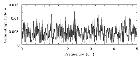
Figure A1: Fourier (semi-amplitude) periodogram for HD 116827.

A.2. LSS3072 $\equiv$ CPD -61$\degr$3692

This object appears in the catalogue of OB stars of Reed (Reed (2003)) and is classified as O9. The magnitudes measured in the framework of the present work are given in Table A3, available at the CDS. It is clearly variable and the light curve is plotted against time in Fig. A2. A search for periods results in the detection of the possible frequency $\nu$ = 0.1092 d^-1 ($P$ = 9.16 d) for each of the four bandpasses and for the combined data (semi-amplitude 0.023 mag in $B$, 0.023 in $V$, 0.024 in $R$ and 0.023 in $I$). Two bumps are clearly present in Fig. A2. A few discrepant data points are present at HJD 2 451 999.71 and at HJD 2 452 027.54. The deletion of these data points does not change the result of the period search. However, it is worth noticing that they are separated by some three entire cycles and could thus be related to the possible main period. We have no particular reason to reject these possible outliers.

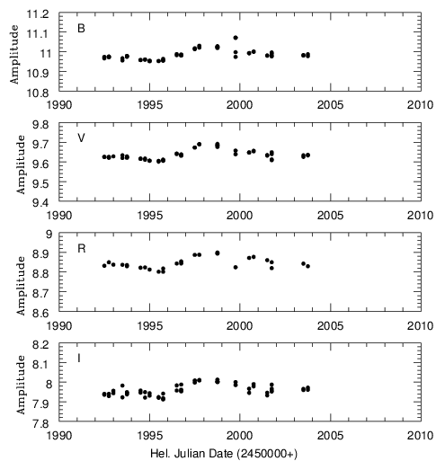
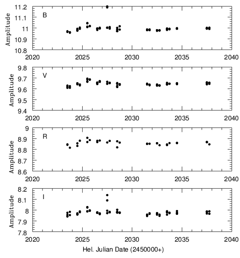
Figure A2: Light curve of LSS 3072.