Orbital selective pairing and superconductivity in iron selenides

Abstract

An important challenge in condensed matter physics is understanding iron-based superconductors. Among these systems, the iron selenides hold the record for highest superconducting transition temperature and pose especially striking puzzles regarding the nature of superconductivity. The pairing state of the alkaline iron selenides appears to be of $d$-wave type based on the observation of a resonance mode in neutron scattering, while it seems to be of $s$-wave type from the nodeless gaps observed everywhere on the Fermi surface (FS). Here we propose an orbital-selective pairing state, dubbed $s\tau_{3}$, as a natural explanation of these disparate properties. The pairing function, containing a matrix $\tau_{3}$ in the basis of $3d$-electron orbitals, does not commute with the kinetic part of the Hamiltonian. This dictates the existence of both intraband and interband pairing terms in the band basis. A spin resonance arises from a $d$-wave-type sign change in the intraband pairing component whereas the quasiparticle excitation is fully gapped on the FS due to an $s$-wave-like form factor associated with the addition in quadrature of the intraband and interband pairing terms. We demonstrate that this pairing state is energetically favored when the electron correlation effects are orbitally selective. More generally, our results illustrate how the multiband nature of correlated electrons affords unusual types of superconducting states, thereby shedding new light not only on the iron-based materials but also on a broad range of other unconventional superconductors such as heavy fermion and organic systems.

I Introducton

Unconventional superconductivity is driven by electron-electron interactions, instead of electron-phonon couplings Anderson (2007). It occurs in a variety of strongly correlated electron systems, with the iron-based superconductors (FeSCs) representing a prototype case  Kamihara et al. (2008); Johnston (2010); Si et al. (2016); Wang and Lee (2011); Hosono and Kuroki (2015); Hirschfeld (2016). The field of FeSC started with most of the efforts being directed toward the iron pnictide class. The normal state was found to be a bad metal, with room-temperature resistivity reaching the Mott-Ioffe-Regel limit Johnston (2010); Qazilbash et al. (2009), suggesting the importance of electron correlations Si and Abrahams (2008); Yin et al. (2011). More recently, the focus has been shifted to iron selenide systems. The reasons are manifold. They have the highest $T_{c}$ Wang et al. (2012a); Lee et al. (2014), they show even stronger electron correlations, and, as we discuss here, their superconductivity is highly unusual.

The puzzle of the superconducting pairing state is highlighted by the “122” alkaline iron selenides. These systems have a $T_{c}$ of about $31$ K at ambient pressure. They have only electron Fermi pockets, lacking the hole pockets that exist in the iron pnictides at the center of the Brillouin Zone (BZ) Mou et al. (2011); Zhang et al. (2013); Wang et al. (2011). Angle-resolved photoemission spectroscopy (ARPES) experiments show that the quasiparticle dispersion is fully gapped on all the parts of the FS Mou et al. (2011); Zhang et al. (2013); Wang et al. (2011), including a small electron Fermi pocket at the center of the BZ Xu et al. (2012); Wang et al. (2012b). This is compatible with the usual $s$-wave $A_{1g}$ pairing state, but not with the usual $d$-wave $B_{1g}$ state (which would produce nodes on the small electron Fermi pocket near the center of the BZ). On the other hand, inelastic neutron scattering experiments Park et al. (2011); Friemel et al. (2012) observe a sharp resonance peak around the wavevector $(\pi,\pi/2)$. It is consistent with a pairing function that changes sign Eschrig (2006) between the two Fermi pockets at the edge of the BZ, such as would occur in a $d$-wave $B_{1g}$ state, but not in the usual $s$-wave $A_{1g}$ case.

In this work, we demonstrate how an orbital-selective pairing state, dubbed $s\tau_{3}$, exhibits properties that are commonly associated with a $d$-wave $B_{1g}$ state or a $s$-wave $A_{1g}$ state. The key to the emergence of this superconducting state is the multiband nature of the FeSCs. This is associated with the multiplicity of $3d$ electron orbitals, whose conceptual importance follows the tradition wherein new physics develops out of extra degrees of freedom, similar, for instance, to the way the so-called valley quantum number in the electronic structure introduces new topological properties Schaibley et al. (2016). It is important for the FeSCs that there are multiple orbitals at play in the neighborhood of the Fermi level. Thus there is reason to expect that correlation effects will be different for different orbitals. In fact, there is evidence for orbitally-selective Mott behavior in the iron selenides  Yi et al. (2015, 2013); Wang et al. (2014); Ding et al. (2014); Li et al. (2014) and, thus, orbital selectivity is to be expected for pairing as well.

For strongly correlated superconductivity, Cooper pairing is naturally considered in an orbital basis due to the tendency of the electrons to avoid the dominating Coulomb repulsions. Considering a basis formed from all five $3d$-orbitals, the $s\tau_{3}$ state has an $s$-wave form factor, but transforms as a $d$-wave $B_{1g}$ state. As such, it represents an energetically-favored reconstruction of the conventional $s$-wave and $d$-wave pairing states when they are quasi-degenerate, due to frustrated antiferromagnetic interactions Yu et al. (2013). The pairing function incorporates a matrix $\tau_{3}$ in the $3d_{xz},3d_{yz}$ subspace, which does not commute with the kinetic term of the Hamiltonian. Consequently, in the band basis, it must also have a matrix structure, which contains both intraband and interband terms. This allows the intraband pairing component to have a $d$-wave sign change, while the addition in quadrature of the intraband and interband pairing terms is nonzero everywhere on the FS. Thereby, the spin excitations show a $(\pi,\pi/2)$ resonance while the quasiparticle excitations as measured by ARPES are fully gapped on the Fermi surface.

II Result

Orbital selectivity in the normal state of iron selenides:   In the normal state, ARPES has provided evidence not only for the existence of the orbital degree of freedom but also for strong orbital-selective correlation effects in the iron selenides. These materials include the alkaline iron selenides, the Te-doped “11” iron selenides FeSe, and the monolayer FeSe on the SrTiO₃ substrate Yi et al. (2015, 2013); Wang et al. (2014); Ding et al. (2014); Li et al. (2014). The effective quasiparticle mass normalized by its non-interacting counterpart, $m^{*}/m_{band}$ is on the order of $3-4$ for the $3d_{xz,yz}$ orbitals, but is as large as $20$ for the $3d_{xy}$ orbital Yi et al. (2015, 2013); Liu et al. (2015). Such orbital selectivity has also been the subject of extensive recent theoretical studies  Yu and Si (2011, 2013); de’ Medici et al. (2014). All of these aspects make it natural to study orbital dependent  R.Yu et al. (2014); Yin et al. (2014); Ong et al. (2016) and related  Hao and Hu (2014) superconducting pairing. We are thus motivated to address the hitherto unexplored question, viz. whether there exists an orbital-selective pairing state which can reconcile the seemingly contradictory properties observed in the iron-selenide superconductors. We also examine the stability of such a pairing state at the level of an effective Hamiltonian for studying superconductivity, in which we incorporate the orbital-selectivity in the short-range exchange interactions (see Supplementary Information (SI)).

Orbital-selective $s\tau_{3}$ pairing state – a simplified case:   We first discuss the structure and properties of the $s\tau_{3}$ pairing state in a simplified two-orbital $d_{xz},d_{yz}$ system. This illustrates how features typically associated with both standard structure-less $s$- and $d$-wave states can simultaneously arise. The salient features of the two-orbital model are illustrated in Fig. 1.

We consider spin-singlet pairing in the orbital basis, in the case of two orbitals $3d_{xz}$, $3d_{yz}$  Raghu et al. (2008). The Hamiltonian, incorporating the $s\tau_{3}$ pairing term, is given by

$$\hat{H}= \sum_{\boldsymbol{k}}\psi^{\dagger}_{\boldsymbol{k}}\big{(}\hat{H}_{\text{Kinetic}}(\boldsymbol{k})+\hat{H}_{\text{Pair}}(\boldsymbol{k})\big{)}\psi_{\boldsymbol{k}}$$

$$\hat{H}_{\text{Kinetic}}= \big{(}\xi_{+}(\boldsymbol{k})\otimes\tau_{0}+\xi_{-}(\boldsymbol{k})\otimes\tau_{3}+\xi_{xy}(\boldsymbol{k})\otimes\tau_{1}\big{)}\otimes\sigma_{0}\otimes\gamma_{3}$$

$$\hat{H}_{\text{Pair}}= \Delta_{0}g_{x^{2}y^{2}}(\boldsymbol{k})\otimes\tau_{3}\otimes\sigma_{0}\otimes\gamma_{1},$$ (1)

where $\psi^{\dagger}_{\boldsymbol{k}}=(c^{\dagger}_{\boldsymbol{k}i\sigma},c_{-\boldsymbol{k}j\sigma^{\prime}}(i\sigma_{2})_{\sigma^{\prime}\sigma})$ is equivalent to a Nambu spinor where $i,j$ are orbital indices (SI Section). The $\tau_{i},\sigma_{i}$, and $\gamma_{i},(i=0,\ldots,4)$ 2 x 2 Pauli matrices represent orbital iso-spin, spin, and Nambu indices, respectively. The $\xi_{+},\xi_{-}$, and $\xi_{xy}$ factors appearing in the kinetic part belong to the $A_{1g},B_{1g}$, and $B_{2g}$ irreducible representations of the $D_{4h}$ point-group. Their exact forms, as well as the resulting electron bands are given in the SI.

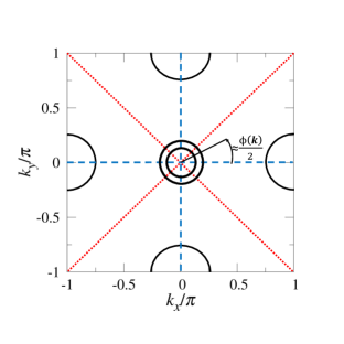
Figure 1: Schematic illustration of the two-orbital $s\tau_{3}$ pairing in a 1-Fe Brillouin Zone (BZ), which is obtained by unfolding the 2D crystallographic BZ cell in the conventional fashion Nica et al. (2015). The solid lines indicate typical Fermi pockets for the Fe-based superconductors. The dotted, red lines indicate the zeroes specific to the intraband pairing ( $\xi_{-}$) while the dashed, blue lines mark the zeroes specific to the interband pairing ( $\xi_{xy}$). The intra- and inter- band components do not vanish at the same subset of $\boldsymbol{k}$, ensuring there is always a non-zero pairing given by either of the two components on the entire Fermi surface. For $\text{max}(\xi_{-})\approx\text{max}(\xi_{xy})$ the angle $\phi(\boldsymbol{k})$ (Eqs. 5-7) can be roughly identified with twice the winding angle shown for fixed $|\boldsymbol{k}|$. In addition, there is a sign change between the intraband pairing along the two pockets at the edge of the BZ, a condition necessary to the formation of a resonance in the spin excitation spectrum at the wavevector $\boldsymbol{q}=(\pi,\pi/2)$ observed in experiment Dai (2015).

The even-parity, spin-singlet candidate $s\tau_{3}$ pairing function with non-trivial orbital structure is included in the $\hat{H}_{\text{Pair}}$ term in Eq. II. While $\Delta_{0}$ is a (generally) complex number, we choose a real amplitude for convenience. The form factor $g_{x^{2}y^{2}}(\boldsymbol{k})$ is parity-even and belongs to the $A_{1g}$ representation of the $D_{4h}$ point group. In the absence of spin-orbit coupling, the rotational properties of the $s\tau_{3}$ pairing are of $B_{1g}$ symmetry. The latter is entirely determined by the tensor product of the $g_{x^{2}y^{2}}(\boldsymbol{k})$ (s-wave) form factor and the $\tau_{3}$ orbital matrix. To illustrate, under a $C_{4z}$ rotation, the form-factor is invariant, while the $\tau_{3}$ matrix transforms as a rank-two $B_{1g}$ tensor representation of the point-group, i.e. it changes sign. We note that the anti-symmetry under exchange is guaranteed by the spin-singlet nature, together with the even-parity of the form factor. Since the spin-structure is not essential for the following arguments, we shall henceforth omit the explicit $\sigma_{0}$ matrix.

The non-trivial characteristics of this pairing are consequences of the commutator $\left[\hat{H}_{\text{Kinetic}},\hat{H}_{\text{Pair}}\right]\neq 0$ for general momentum $\boldsymbol{k}$. We use the notation of Ref. 34, and rewrite the Hamiltonian Eq. II as follows

$$\hat{H}= \sum_{\boldsymbol{k}}\psi^{\dagger}({\boldsymbol{k}})\big{[}\left(\xi_{+}(\boldsymbol{k})\tau_{0}+\vec{B}({\boldsymbol{k}})\cdot\vec{\tau}\right)\otimes\gamma_{3}$$

$$+\left(\vec{d}({\boldsymbol{k}})\cdot\vec{\tau}\right)\otimes\gamma_{1}\big{]}\psi({\boldsymbol{k}}),$$ (2)

where

$$\vec{B}(\boldsymbol{k})= \left(\xi_{xy}(\boldsymbol{k}),0,\xi_{-}(\boldsymbol{k})\right)$$

$$\vec{d}(\boldsymbol{k})= \left(0,0,\Delta_{0}g_{x^{2}y^{2}}(\boldsymbol{k})\right).$$ (3)

This is formally similar to a Balian-Werthamer form  Balian and Werthamer (1963); Leggett (1975); Sigrist and Ueda (1991) (see SI for more details), with the $\vec{B}(\boldsymbol{k})$ factor being analogous to a $\boldsymbol{k}$-dependent spin-orbit coupling. To account for the non-commuting $\hat{H}_{\text{Kinetic}}$ and $\hat{H}_{\text{Pair}}$, we write the square of the Hamiltonian matrix:

$$\hat{H}^{2}= \sum_{\boldsymbol{k}}\left[\xi_{+}(\boldsymbol{k})\tau_{0}+\left(\vec{B}_{\boldsymbol{k}}\cdot\vec{\tau}\right)\right]^{2}\otimes\gamma_{0}+\left|\vec{d}(\boldsymbol{k})\right|^{2}\tau_{0}\otimes\gamma_{0}$$

$$+2i\left(\vec{B}(\boldsymbol{k})\times\vec{d}(\boldsymbol{k})\right)\cdot\vec{\tau}\otimes i\gamma_{2}.$$ (4)

where the well-known relation $\big{(}\vec{a}\cdot\vec{\tau}\big{)}\big{(}\vec{b}\cdot\vec{\tau}\big{)}=\vec{a}\cdot\vec{b}+i\big{(}\vec{a}\times\vec{b}\big{)}\cdot\vec{\tau}$ was used. The first two terms, proportional to the $\gamma_{0}$ Nambu matrix, are the squares of the kinetic Hamiltonian and of a pairing contribution with no essential structure in orbital space, given by $\left|\vec{d}(\boldsymbol{k})\right|^{2}$. The latter is an effective amplitude of the pairing interactions and, as such, is proportional to the square of the s-wave like $g_{x^{2}y^{2}}$ form factor, as can be seen from Eq. 3. Together with the kinetic part, it amounts to the usual (and sole) contribution to the Bogoliubov-de Gennes (BdG) quasiparticle spectrum, whenever $\left[\hat{H}_{\text{Kinetic}},\hat{H}_{\text{Pair}}\right]=0$ for all $\boldsymbol{k}$. The last term in Eq. II reflects the non-commuting $\hat{H}_{\text{Kinetic}}$ and $\hat{H}_{\text{Pair}}$. Since the Nambu matrices $\gamma_{0}$ and $i\gamma_{2}$ commute, $\hat{H}^{2}$ in Eq. II can be easily expressed in block diagonal form (SI). The resulting Bogoliubov-de Gennes (BdG) bands are given by

$$E_{\pm}(\boldsymbol{k})=\sqrt{\left(\sqrt{\xi^{2}_{+}(\boldsymbol{k})+\left|\vec{d}(\boldsymbol{k})\right|^{2}\text{sin}^{2}\phi(\boldsymbol{k})}\pm\left|\vec{B}(\boldsymbol{k})\right|\right)^{2}+\left|\vec{d}(\boldsymbol{k})\right|^{2}\left(1-\text{sin}^{2}\phi(\boldsymbol{k})\right)}$$ (5)

where

$$\text{sin}\phi(\boldsymbol{k})=\frac{\xi_{xy}(\boldsymbol{k})}{\left|\vec{B}(\boldsymbol{k})\right|}=\frac{\xi_{xy}(\boldsymbol{k})}{\sqrt{\xi^{2}_{-}(\boldsymbol{k})+\xi^{2}_{xy}(\boldsymbol{k})}}.$$ (6)

The terms proportional to $\sin\phi(\boldsymbol{k})$ reflects the non-Abelian aspect of the pairing state. Note that Eq. 5 corresponds to the sum of two positive semi-definite terms. For general $\vec{d}(\boldsymbol{k})$ we see that nodes can appear only when both terms in the square root vanish. The second of these goes to zero when either $\text{sin}\phi(\boldsymbol{k})=1$ or, trivially, when $\left|\vec{d}(\boldsymbol{k})\right|=0$. This latter case occurs when the FS intersects the lines of zeros of the $g_{x^{2}y^{2}}$ form factor. With the FeSCs in mind, we ignore this simple case in the following. Alternately, when $\text{sin}\phi(\boldsymbol{k})=1$, the dispersion reduces to

$$E_{\pm}(\boldsymbol{k})=\left|\sqrt{\xi^{2}_{+}(\boldsymbol{k})+\left|\vec{d}(\boldsymbol{k})\right|^{2}}\pm\left|\vec{B}(\boldsymbol{k})\right|\right|.$$ (7)

On the FS, we have $\xi^{2}_{+}(\boldsymbol{k})=\left|\vec{B}(\boldsymbol{k})\right|^{2}$ (see SI). Thus, there are no nodes on the FS.

We note that away from the FS, Eq. 7 does not in general guarantee the absence of nodes. However, because the lifetime of quasiparticles away from the FS will be finite, the corresponding contributions to thermodynamical properties will be much weaker compared to the case of nodes on the FS.

In the band basis, the kinetic part of the Hamiltonian is diagonalized. Given that the kinetic and pairing parts do not commute with each other, the two cannot be simultaneously diagonalized. Thus, the pairing part must contain an interband component. To see this, we apply a canonical transformation which diagonalizes the kinetic part (see the SI), but which also transforms the pairing into

$$\hat{H}_{\text{Pair}}(\boldsymbol{k})=\Delta_{1}(\boldsymbol{k})\alpha_{3}+\Delta_{2}(\boldsymbol{k})\alpha_{1}$$ (8)

where $\alpha_{1,3}$ are Pauli matrices corresponding to inter- and intra-band pairing terms. The two components are given by

$$\Delta_{1}(\boldsymbol{k})= -\Delta_{0}g_{x^{2}y^{2}}(\boldsymbol{k})\frac{\xi_{-}(\boldsymbol{k})}{\sqrt{\xi^{2}_{-}(\boldsymbol{k})+\xi^{2}_{xy}(\boldsymbol{k})}}$$

$$\Delta_{2}(\boldsymbol{k})= -\Delta_{0}g_{x^{2}y^{2}}(\boldsymbol{k})\frac{\xi_{xy}(\boldsymbol{k})}{\sqrt{\xi^{2}_{-}(\boldsymbol{k})+\xi^{2}_{xy}(\boldsymbol{k})}}.$$ (9)

The band-diagonal $\alpha_{3}$ and band off-diagonal $\alpha_{1}$ pairing components have $d(x^{2}-y^{2})$ and $d(xy)$ form factors, respectively. As illustrated in Fig. 1, these have nodes along the diagonals and axes of the BZ, respectively. Because the two matrices $\alpha_{1,3}$ anti-commute, the single-particle excitation energy depends on the addition in quadrature of the two pairing amplitudes $\Delta_{1}(\boldsymbol{k})$ and $\Delta_{2}(\boldsymbol{k})$. This ensures that the excitation gap is nodeless on the entire Fermi surface.

As can be seen from Eqs. 8, 9, the band-index diagonal term changes sign about the diagonals ($k_{x}=\pm k_{y}$) of the BZ, as dictated by the $d(x^{2}-y^{2})$ nature of the intraband component. Thus, the intraband pairing component does indeed change sign between the two electron Fermi pockets at the BZ boundaries. It ensures that this type of pairing is conducive to the formation of a resonance with a wavevector that connects the two electron Fermi pockets.

We stress that the two main features of the $s\tau_{3}$ pairing, i.e. the formation of a gap on the FS and the sign-change in the intraband component, cannot be reconciled by the more typical pairing candidates, which lack an orbital structure. In the context of our two-orbital model, the $s\otimes\tau_{0}$ and $d\otimes\tau_{0}$ candidate states, corresponding to the typical orbitally-trivial s and d-wave pairings, commute with $\hat{H}_{\text{Kinetic}}$. Consequently, they are associated with intraband pairing only. As such, neither of the two types can induce a nodeless gap and account for the sign change required for the spin-resonance.

Orbital-selective $s\tau_{3}$ pairing state – the case of iron selenides:   Superconductivity in the alkaline iron selenides, like in the related case of the iron pnictides, involves all five Fe-$3d$ orbitals. Thus, it is important to consider the five-orbital case to address i) whether the $s\tau_{3}$ pairing state is energetically favored compared to the more conventional pairing states and ii) whether it captures the essential properties of this pairing state as they pertain to the iron selenide superconductors.

To study the stability of the $s\tau_{3}$ pairing state, we start from two previously discussed aspects of the FeSCs. We do so in terms of a strong-coupling approach to superconductivity, in light of the strong correlation effects  Si and Abrahams (2008); Yin et al. (2011); Fang et al. (2008); Xu et al. (2008); Seo et al. (2008); Moreo et al. (2009); Chen et al. (2009); Yang et al. (2013); Berg et al. (2009); Lv et al. (2010); Bascones et al. (2012); de’ Medici et al. (2014) that are especially clear-cut for the iron selenides  Yi et al. (2015, 2013); Liu et al. (2015). This approach is described in the SI, with superconductivity driven by short-range interactions. The latter include the antiferromagnetic interactions between the nearest-neighbor (NN, $J_{1}^{\alpha}$) and next-nearest-neighbor (NNN,$J_{2}^{\alpha}$) Fe sites on their square lattice, for the three most relevant orbitals, $\alpha=$ $3d_{xz}$, $3d_{yz}$, and $3d_{xy}$. We reiterate that we will analyze the model in the 1-Fe unit cell and the corresponding BZ.

One of the known aspects of the FeSCs is the large parameter regime where the conventional $d$-wave $B_{1g}$ and $s$-wave $A_{1g}$ pairing states are quasi-degenerate  Yu et al. (2013); Graser et al. (2009). In terms of a model with short-range antiferromagnetic interactions, this occurs in the regime of magnetic frustration with $J_{2}$ being comparable to $J_{1}$ Yu et al. (2013), a condition that is evidenced by both theoretical considerations and experimental measurements  Si et al. (2016); Dai (2015). To quantify this effect, we introduce the ratio $A_{L}\equiv J_{2}/J_{1}$ to describe the relative strength of these two interactions. For a proof-of-concept demonstration, we analyze the phase diagram by taking the $J_{2}/J_{1}$ axis to be a cut in the parameter space along which $A_{L}$ is the same for the different $3d$ orbitals. The quasi-degeneracy arises when $A_{L}\sim 1$.

The second well-known property of the FeSCs is orbital selectivity, as described above. Our effective model incorporates an exchange orbital-anisotropy factor $A_{O}=J_{1}^{xy}/J_{1}^{xz/yz}=J_{2}^{xy}/J_{2}^{xz/yz}$, and reflects the orbital selectivity by $A_{O}$’s deviation from $1$. For the iron selenides, $A_{O}$ is expected to be considerably smaller than $1$ (see SI).

We are now in position to discuss how the $s\tau_{3}$ pairing state emerges in a range of parameters where the $s-$ and $d-$wave pairing channels are quasi-degenerate. Within the 5-orbital $t-J_{1}-J_{2}$ model, we focus on the case with a kinetic part appropriate for the alkaline iron selenides K_yFe_2-xSe₂ although similar behavior emerges in the cases appropriate for the iron pnictides and single-layer FeSe (see SI). We present our results for the case of orbital-diagonal exchange interactions. The inter-orbital exchange interactions have only negligible effects on the pairing amplitudes, as demonstrated in the SI.

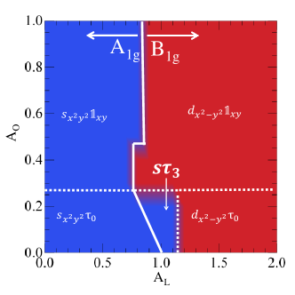
(a)

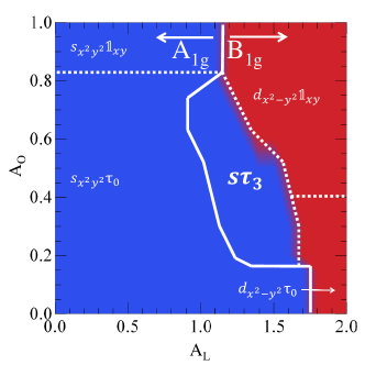
(b)

Figure 2: Phase diagrams based on the leading pairing amplitudes given by self-consistent calculations with fixed $J_{2}=1$ and tight-binding parameters appropriate to (a) alkaline iron selenides, and (b) iron pnictides. The tight-binding parameters used can be found in Ref. 27. The blue shaded areas correspond to dominant pairing channels with an $s_{x^{2}y^{2}}$ form factor while the red shading covers those with a $d_{x^{2}-y^{2}}$ form factor. The continuous line separates regions where the pairing belongs to the $A_{1g}$ and the $B_{1g}$ representations respectively. The $1\times 1$ matrix in the $d_{xy}$ subspace is represented by $\boldsymbol{1}_{xy}$. The orbital-selective $s\tau_{3}$ pairing occurs for $A_{O}<1$, $A_{L}$ near 1 in all cases.

The phase diagram for the alkaline iron selenides is shown in Fig. 2 (a). In the absence of orbital selectivity, $A_{O}=1$, it is known that small and large $A_{L}$ promote the $s_{x^{2}y^{2}}\otimes\tau_{0},{A_{1g}}$ and $d_{x^{2}-y^{2}}\otimes\tau_{0},B_{1g}$, both defined in the $d_{xz}$, $d_{yz}$ subspace Yu et al. (2013). Increasing the orbital selectivity, with $A_{O}$ decreasing from $1$, these two limiting regimes remain essentially unchanged. However, in the magnetically frustrated regime $A_{L}\sim 1$, the $s_{x^{2}y^{2}}\otimes\tau_{0},{A_{1g}}$ and $d_{x^{2}-y^{2}}\otimes\tau_{0},B_{1g}$ become quasi-degenerate. When $A_{O}$ is sufficiently smaller than $1$, the $s\tau_{3}$ pairing state becomes the dominant channel in the intermediate regime. Similar phase diagrams are obtained for the iron pnictides and single-layer FeSe shown in Figs. 2 (b) and S1 (SI), respectively. A typical dominant $s\tau_{3}$ pairing case is shown in Fig. S2 in the SI for a number of subleading symmetry-allowed channels Goswami et al. (2010) for alkaline iron selenide dispersion with fixed $J_{2}/J_{1}=1.5$, $A_{O}=0.3$ and varying $A_{L}$ (horizontal axis).

Having established the stability of the $s\tau_{3}$ pairing state, we now address its salient properties. We first consider the spin-excitation spectrum. In Fig. 3 we show the dynamical spin susceptibility at wave-vector $\boldsymbol{q}=(\pi,\pi/2)$ for $J_{2}=1.5$. We note the complicated frequency behavior which can be traced to the anisotropy in the effective gap affecting both the coherence factors and the position of minimum in quasi-particle energy. We show the minimum and maximum particle-hole (p-h) thresholds corresponding to twice the minimum and twice the maximum gaps. As suggested by Figs. 4 (a) and (b), states connected by $\boldsymbol{q}=(\pi,\pi/2)$ would correspond to a p-h threshold given roughly by the sum of the minimum and maximum gap. A sharp feature appears below this threshold, confirming the existence of the resonance for $\boldsymbol{q}=(\pi,\pi/2)$ as found in experiments on the alkaline iron selenides Park et al. (2011); Friemel et al. (2012); Dai (2015). The resonance at this wavevector originates from the sign change of the intraband pairing component across the two Fermi pockets at the edge of the BZ, around $(\pm\pi,0)$ ($\delta$) and $(0,\pm\pi)$, as illustrated in Fig. 4 (a), and further discussed in the SI. Without such a sign change, there cannot be a sharp resonance below the p-h threshold energy.

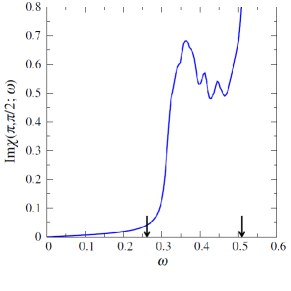
Figure 3: The imaginary part of the dynamical spin susceptibility for the alkaline iron selenides at wave-vector $\boldsymbol{q}=(\pi,\pi/2)$, for a dominant $s\tau_{3}$ pairing for parameters $J_{2}=1.5$, $A_{O}=0.3,A_{L}=0.9$. The arrows show twice the minimum and maximum gaps (see Fig. 4 (b)). There is a sharp feature ar $\omega\approx 0.36$ within the bounds of twice the effective gap and below the p-h threshold of roughly 0.41 associated with this wavevector.

We next turn to the quasiparticle excitation spectrum. Fig. 4 (b) shows the gap at the FS as a function of winding angle $\theta$. It clearly illustrates the node-less dispersion as the gap is nonzero for all $\theta$.

The electron dispersion considered here does not produce any Fermi pockets close to $\Gamma$ in the BZ. This is in contrast to ARPES experiments on K_yFe_2-xSe₂ Zhang et al. (2011); Liu et al. (2012) which show a small electron pocket near $\Gamma$. Because this electron pocket has very small spectral weight, it is to be expected that even if such a pocket were included, the dominant $s\tau_{3}$ pairing will still arise; moreover, the gap on this Fermi pocket will be node-less as discussed in the two-orbital case. To substantiate this, we consider the results for the iron pnictides class, which do have significant (albeit hole) Fermi pockets at the zone center yet exhibit a full gap. In Figs. 5 (a), (b) we show the FS and the gaps as functions of winding angle $\theta$ for $A_{O}=0.5$ and $A_{L}=1.3$ corresponding to a dominant $s\tau_{3}$ pairing. The gap along $\beta$ is finite and exhibits an anisotropy consistent with the two orbital results in Eq. 5. In the latter case, at winding angle $\theta=0$, $\text{sin}\phi=0$ and the spectrum has a minimum/maximum gap for $E_{+/-}$. As $\theta$ is increased the $\left|\vec{B}(\boldsymbol{k})\times\vec{d}(\boldsymbol{k})\right|^{2}$ term increases reaching a maximum at $\theta=\pi/4$. Here the gap is maximum/minimum for $E_{+/-}$. This is consistent with the anisotropy in the gap shown in Fig. 5.

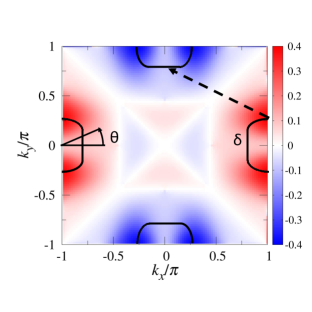
(a)

(b)

Figure 4: (a) The FS (solid line) and the real intra-band pairing for the band generating the $\delta$ pockets at the edge of the BZ for a dispersion typical of the alkaline iron selenides. Note the clear change in sign between pockets separated by the BZ diagonal. The dashed arrow indicates the $\boldsymbol{q}=(\pi,\pi/2)$ wave-vector associated with the resonance in the spin spectrum found in experiment Dai (2015). (b) The size of the gap along the $\delta$ pocket. Both figures are for $J_{2}=1.5$, $A_{O}=0.3,A_{L}=0.9$ with dominant $s\tau_{3}$ pairing.

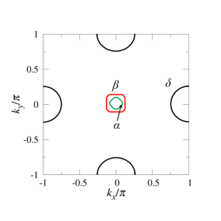
(a)

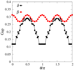
(b)

Figure 5: (a) FS for the iron pnictides which includes hole pockets around the $\Gamma$ point with dominant $s\tau_{3},B_{1g}$ for $J_{2}=1,A_{L}=1.3,A_{O}=0.5$.The tight-binding parameterscan be found in Ref. 27. (b) The gaps along the $\beta$ and $\delta$ pockets close to the center and edge of the BZ. A similar gap forms around the $\alpha$ pocket.

III Discussion

Several remarks are in order. First, the full gap and the sign change of the intraband pairing component discussed above provide evidence that, with strong orbital selectivity, the $s\tau_{3}$ pairing in a realistic five-orbital model has a behavior very similar to that of the two-orbital case.

Second, with the short-range $J_{1}-J_{2}$ interactions driving superconductivity, pairing involves the electronic states over an extended range of energy about the Fermi energy. The energy window can be determined from the zone-boundary spin excitation energies, which are on the order of $200$ meV for most iron selenides (and pnictides) Dai (2015). This is important for the consideration of the quasiparticle excitation gap at the small electron pocket of K_yFe_2-xSe₂ near the origin of the Brillouin zone. According to the ARPES experiments Zhang et al. (2011); Liu et al. (2012) this Fermi pocket contains Fe $3d_{xy}$ and Se $4p_{z}$ orbitals ($\alpha$ band), while the hole ($\beta$) bands containing both $3d_{xz}$ and $3d_{yz}$ orbitals and are only about $60$-$80$ meV below the Fermi energy. We therefore expect that both the intraband and interband pairing components will be significant for this part of the Brillouin zone and the mechanism advanced here will make the quasiparticle excitations to be fully gapped for this small electron pocket.

Third, within our approach both the iron selenides and pnictides are bad metals in the regime of quasi-degenerate $s-$ and $d-$wave pairings. However, the iron selenides have stronger correlations, which will lead to a larger ratio of the exchange interaction to renormalized kinetic energy (note that the renormalized bandwidth goes to zero when a bad metal approaches the electron localization transition) and, correspondingly Yu et al. (2013), larger pairing amplitudes. We expect this will contribute to the larger maximum $T_{c}$ observed in the iron selenides than in the iron pnictides. Relatedly, the alkaline iron selenides have a stronger orbital selectivity than the iron pnictides, and we thus expect that the $s\tau_{3}$ pairing is more likely realized in the former than in the latter.

Fourth, it is instructive to compare the mechanism advanced here with a conventional means of relieving quasi-degenerate $s-$ and $d-$wave pairing states with trivial orbital structure, which consists in linearly superposing the two into an $s+id$ state. The latter, breaking the time-reversal symmetry, would be stabilized at temperatures sufficiently below the superconducting transition temperature. By contrast, the $s\tau_{3}$ pairing state preserves the time-reversal symmetry. It is an irreducible representation of the point group, and is therefore stabilized as the temperature is lowered immediately below the superconducting transition. Thus, the emergence of the intermediate $s\tau_{3}$ pairing state represents a new means to relieve the quasi-degeneracy through the development of orbital selectivity.

Finally, the nodeless $d$-wave nature of $s\tau_{3}$ may shed new light on other strongly correlated multi-band superconductors. For instance, one of the striking puzzles emerging in heavy fermion superconductors is the simultaneous exhibition of a variety of $d-$wave characteristics and of a gap in the lowest-energy excitation spectrum Kittaka et al. (2014). Whether a multiband pairing state such as $s\tau_{3}$ provides a systematic understanding of such properties is an intriguing open question for future studies.

To summarize, we have demonstrated that an orbital-selective $s\tau_{3}$ pairing state exhibits properties that would appear mutually exclusive from the conventional perspective where the orbital degrees of freedom are ignored. It provides a natural understanding of the enigmatic properties observed in the alkaline iron selenides. These include the single-particle excitations which are fully gapped on the entire Fermi surface, as observed in ARPES experiments, and a pairing function which changes sign across the electron Fermi pockets at the Brillouin-zone boundary, as indicated by the resonance peak seen near $(\pi,\pi/2)$ in the inelastic neutron scattering experiments. In addition, we have shown that the pairing state is energetically competitive in an orbital-selective model of short-range antiferromagnetic exchange interactions, in the regime where the conventional $s-$ and $d-$wave pairing channels are quasi-degenerate. As such, our understanding of the properties of the iron-selenide superconductors provides evidence that the high-T_c superconductivity in the iron-based materials originates from the antiferromagnetic correlations of strongly correlated electrons. More generally, our work highlights how new classes of unconventional superconducting pairing state emerge in the presence of additional internal degrees of freedom, with properties that cannot otherwise be expected. This new insight may well be important for the understanding of a variety of other strongly correlated superconductors, including the heavy fermion and organic systems.

IV Acknowledgments

We acknowledge useful discussions with E. Abrahams, A. V. Chubukov, G. Kotliar and P. J. Hirschfeld. The authors declare that they have no competing interests. All authors contributed to the research of the work and the writing of the paper. The work has been supported in part by the NSF Grant No. DMR-1611392 and the Robert A. Welch Foundation Grant No. C-1411 (E.M.N. & Q.S.). R.Y. was partially supported by the National Science Foundation of China Grant number 11374361, and the Fundamental Research Funds for the Central Universities and the Research Funds of Renmin University of China. All of us acknowledge the support provided in part by the NSF Grant No. NSF PHY11-25915 at KITP, UCSB. Correspondence and requests for materials should be addressed to E.M.N. (enica@qmi.ubc.ca) or Q.S. (qmsi@rice.edu).

Orbital selective pairing and superconductivity in iron selenides - Supporting Information Emilian M. Nica, Rong Yu, and Qimiao Si

I Two-orbital model

A Tight-binding details

The components of the tight-binding part of the two-orbital Hamiltonian discussed in the main text are given by

$$\xi_{\boldsymbol{k}+}= -(t_{1}+t_{2})(\cos k_{x}+\cos k_{y})$$

$$-4t_{3}\cos k_{x}\cos k_{y},$$ (S1)

$$\xi_{\boldsymbol{k}-}= -(t_{1}-t_{2})(\cos k_{x}-\cos k_{y}),$$ (S2)

$$\xi_{\boldsymbol{k}xy}= -4t_{4}\sin k_{x}\sin k_{y},$$ (S3)

where $t_{1}$,$t_{2}$ and $t_{3}$ are tight-binding parameters. Details can be found in Ref. Raghu et al. (2008). The corresponding band dispersion is in general given by

$$\epsilon_{\pm}(\boldsymbol{k})= \xi_{+}(\boldsymbol{k})\pm\sqrt{\xi^{2}_{-}(\boldsymbol{k})+\xi^{2}_{xy}(\boldsymbol{k})}$$

$$= \xi_{+}(\boldsymbol{k})\pm\left|\vec{B}(\boldsymbol{k})\right|$$ (S4)

The Fermi surface is determined by the condition

$$\epsilon_{\pm}(\boldsymbol{k}_{FS})=0,$$ (S5)

which is equivalent to

$$\xi_{+}(\boldsymbol{k}_{FS})=\mp\left|\vec{B}(\boldsymbol{k}_{FS})\right|.$$ (S6)

B Nambu form

The pairing part written as $\hat{H}_{\text{Pair}}\sim\vec{d}\cdot\vec{\tau}$ is equivalent to a more-conventional Balian-Werthamer form $\left(\tilde{\boldsymbol{d}}\cdot\vec{\tau}\right)\left(i\tau_{2}\right)$ which is conventionally used for pairing functions with non-trivial spin structure. This is so provided that $d_{2}=\tilde{d}_{2}=0$, which is the case for $s\otimes\tau_{3}$ pairing, together with ${d}_{1}\rightarrow\tilde{d}_{3},{d}_{3}\rightarrow-\tilde{d}_{1}$. Formally, this transforms $2i\left(\vec{B}\times\vec{d}\right)\cdot\vec{\tau}$ in the expression for $\hat{H}^{2}$ (Eq. 4 in the main text) to $2\left(\vec{B}\cdot\boldsymbol{\tilde{d}}\right)i\tau_{2}$. The resulting BdG bands are identical, as can be seen by expanding the direct products. Note that, in contrast to the typical spin-triplet pairing, both $\vec{d}$ and $\tilde{d}$ orbital iso-spin vectors are parity-even $\left(\vec{d}(-\boldsymbol{k})=\vec{d}(\boldsymbol{k})\right)$. Together with the spin-singlet nature, this ensures that the Cooper pairs are anti-symmetric under exchange.

In order to better illustrate the effects of the non-trivial orbital structure, we incorporate the spin-singlet nature of the pairing Hamiltonian into a transformed Nambu spinor:

$$\psi^{\dagger}(\boldsymbol{k})=\psi^{\dagger}_{\text{Nambu}}~{}U^{\dagger}$$ (S7)

where

$$\psi^{\dagger}_{\text{Nambu}}(\boldsymbol{k})=(c^{\dagger}_{\boldsymbol{k}i\sigma},c_{-\boldsymbol{k}j\sigma}),$$ (S8)

is the canonical Nambu spinor and

$$U=\frac{1}{2}\big{(}\sigma_{0}\otimes(\gamma_{0}+\gamma_{3})+i\sigma_{2}\otimes(\gamma_{0}-\gamma_{3})\big{)}\otimes\tau_{0}.$$ (S9)

C BdG spectrum

$\hat{H}^{2}$ in Eq. 4 in the main text

$$\hat{H}^{2}= \sum_{\boldsymbol{k}}\left[\xi_{+}(\boldsymbol{k})\tau_{0}+\left(\vec{B}_{\boldsymbol{k}}\cdot\vec{\tau}\right)\right]^{2}\otimes\gamma_{0}+\left|\vec{d}(\boldsymbol{k})\right|^{2}\tau_{0}\otimes\gamma_{0}$$

$$+2i\left(\vec{B}(\boldsymbol{k})\times\vec{d}(\boldsymbol{k})\right)\cdot\vec{\tau}\otimes i\gamma_{2}.$$ (S10)

can be brought to a block-diagonal form in the Nambu indices by applying the transformation

$$\tilde{U}=e^{-i\gamma_{1}(\pi/4)}\otimes\tau_{0}\times\sigma_{0}$$ (S11)

such that

$$\tilde{U}\left(\hat{H}^{2}\right)\tilde{U}^{\dagger}=\begin{pmatrix}\tilde{H}&0\\ 0&\tilde{H}^{T}\end{pmatrix}$$ (S12)

where

$$\tilde{H}=\begin{pmatrix}\xi^{2}_{+}+|\vec{B}|^{2}+\left|d\right|^{2}+2B_{3}\xi_{+}&2B_{1}(\xi_{+}-id_{3})\\ 2B_{1}(\xi_{+}+id_{3})&\xi^{2}_{+}+|\vec{B}|^{2}+\left|d\right|^{2}-2B_{3}\xi_{+}.\end{pmatrix}$$ (S13)

From this expression, one can easily check that the eigenvalues of $\hat{H}$ are given by

$$E_{\pm}(\boldsymbol{k})=\sqrt{\xi^{2}_{+}(\boldsymbol{k})+\left|\vec{B}(\boldsymbol{k})\right|^{2}+\left|\vec{d}(\boldsymbol{k})\right|^{2}\pm\sqrt{4\xi^{2}_{+}(\boldsymbol{k})\left|\vec{B}(\boldsymbol{k})\right|^{2}+4\left|\vec{B}(\boldsymbol{k})\times\vec{d}(\boldsymbol{k})\right|^{2}}.}$$ (S14)

The explicitly positive semi-definite form of Eq. 5 in the main text was obtained by writing

$$\sqrt{4\xi^{2}_{+}(\boldsymbol{k})\left|\vec{B}(\boldsymbol{k})\right|^{2}+4\left|\vec{B}(\boldsymbol{k})\times\vec{d}(\boldsymbol{k})\right|^{2}}= \sqrt{4\xi^{2}_{+}(\boldsymbol{k})\left|\vec{B}(\boldsymbol{k})\right|^{2}+4B^{2}_{1}(\boldsymbol{k})d^{2}_{3}(\boldsymbol{k})}$$

$$= 2\left|\vec{B}(\boldsymbol{k})\right|\sqrt{\xi^{2}_{+}(\boldsymbol{k})+\frac{B^{2}_{1}(\boldsymbol{k})}{\left|\vec{B}(\boldsymbol{k})\right|^{2}}d^{2}_{3}(\boldsymbol{k})}$$

$$= 2\left|\vec{B}(\boldsymbol{k})\right|\sqrt{\xi^{2}_{+}(\boldsymbol{k})+\sin^{2}\phi(\boldsymbol{k})\left|\vec{d}(\boldsymbol{k})\right|^{2}}.$$ (S15)

The square can be completed by adding and subtracting $\sin^{2}\phi(\boldsymbol{k})\left|\vec{d}(\boldsymbol{k})\right|^{2}$.

Alternately, a more conventional form for the BdG dispersion can be obtained from Eq. S14 by adding and subtracting $2\xi_{+}(\boldsymbol{k})\left|\vec{B}(\boldsymbol{k})\right|$ to Eq. I C, and completing the square for the non-interacting bands $\epsilon^{2}_{\pm}$. The result is:

$$E_{\pm}(\boldsymbol{k})=\sqrt{\epsilon^{2}_{\pm}(\boldsymbol{k})+|\vec{d}|^{2}(\boldsymbol{k})\pm|Q|(\boldsymbol{k})},$$ (S16)

where

$$\epsilon_{\pm}(\boldsymbol{k})= \xi_{+}(\boldsymbol{k})\pm|\vec{B}|(\boldsymbol{k})$$

$$= \xi_{+}(\boldsymbol{k})\pm\sqrt{\xi_{-}^{2}(\boldsymbol{k})+\xi^{2}_{xy}(\boldsymbol{k})},$$ (S17)

are the electron bands, and the additional $|Q|$ factor is given by

$$|Q|(\boldsymbol{k})=2|\vec{B}|(\boldsymbol{k})\left(\sqrt{\xi^{2}_{+}(\boldsymbol{k})+\left|\vec{d}(\boldsymbol{k})\right|^{2}\text{sin}^{2}\phi(\boldsymbol{k})}-\xi_{+}(\boldsymbol{k})\right).$$ (S18)

The presence of this additional contribution, due to the non-commuting aspect discussed in the main text, induces a splitting between the two conventionally-gapped BdG bands.

Indeed, if $\left[\hat{H}_{\text{Kinetic}},\hat{H}_{\text{Pair}}\right]\sim\vec{B}\times\vec{d}$ (Eq. 4 in the main text) were to vanish for all $\boldsymbol{k}\in BZ$, the splitting given by $|Q|$ term would be absent as well. This can occur for a $\vec{B}$ vector which is either identically zero or aligned parallel/anti-parallel to $\vec{d}$ for all momenta. In such cases, the remaining first two terms in Eq. S16 would correspond to a quasiparticle spectrum with gaps determined by the amplitude of the pairing, or by the square of the $g_{x^{2}y^{2}}$ form factor in our case. The resulting BdG bands would be identical to those for a simpler $s_{x^{2}y^{2}}\otimes\tau_{0}$ state, which is an example of the $s\pm$ pairing. As in this latter case, nodes would appear only when the form factor vanishes along the $\{\pm\pi/2,k_{y}\},\{k_{x},\pm\pi/2\}$ lines. A FS which does not intersect these lines would consequently be completely gapped. The presence of the last term in Eq. 4 in the main text modifies this simple picture, by introducing the additional splitting of the two conventionally-gapped BdG bands. Furthermore, it is possible that this splitting can be sufficiently strong to induce nodes for the $\epsilon_{-}$ band. As shown by Eq. 5 in the main text, these can emerge along the diagonals $|k_{x}|=|k_{y}|$ of the BZ. However, we stress that, along the FS, this cannot occur, as explained above. We also briefly mention that terms similar to $|\vec{Q}|$ are also known in the context of non-unitary, spin-triplet, time-reversal-symmetry breaking pairings Sigrist and Ueda (1991).

D Band basis

The pairing Hamiltonian ($\hat{H}_{\text{pair}}$) in the band-basis (Eq. 8 in the main text) was obtained from

$$\left(V(\boldsymbol{k})\otimes\sigma_{\sigma_{0}}\right)\hat{H}_{\text{pair}}(\boldsymbol{k})\left(V^{T}(\boldsymbol{k})\otimes\sigma_{0}\right),$$ (S19)

where

$$V(\boldsymbol{k})=\begin{pmatrix}\frac{\xi_{-}-\sqrt{\xi_{-}^{2}+\xi_{xy}^{2}}}{\sqrt{\xi^{2}_{xy}+\left(\xi_{-}-\sqrt{\xi_{-}^{2}+\xi_{xy}^{2}}\right)^{2}}}&\frac{\xi_{-}+\sqrt{\xi_{-}^{2}+\xi_{xy}^{2}}}{\sqrt{\xi^{2}_{xy}+\left(\xi_{-}+\sqrt{\xi_{-}^{2}+\xi_{xy}^{2}}\right)^{2}}}\\ \frac{\xi_{xy}}{\sqrt{\xi^{2}_{xy}+\left(\xi_{-}-\sqrt{\xi_{-}^{2}+\xi_{xy}^{2}}\right)^{2}}}&\frac{\xi_{xy}}{\sqrt{\xi^{2}_{xy}+\left(\xi_{-}+\sqrt{\xi_{-}^{2}+\xi_{xy}^{2}}\right)^{2}}}.\end{pmatrix}.$$ (S20)

is chosen such that $V\hat{H}_{\text{Kinetic}}V^{\dagger}$ is diagonal. It can be recast as

$$V(\boldsymbol{k})=\frac{1}{\sqrt{2}}\begin{pmatrix}-\sqrt{1-\cos{\phi(\boldsymbol{k})}}&\sqrt{1+\cos{\phi(\boldsymbol{k})}}\\ \sqrt{1+\cos{\phi(\boldsymbol{k})}}&\sqrt{1-\cos{\phi(\boldsymbol{k})}}\end{pmatrix},$$ (S21)

where

$$\cos\phi(\boldsymbol{k})=\frac{\xi_{-}(\boldsymbol{k})}{\sqrt{\xi_{-}^{2}+\xi_{xy}^{2}}}.$$ (S22)

The transformation on $\hat{H}_{\text{Pair}}$ is formally equivalent to the improper rotation

$$\vec{d}^{\prime}(\boldsymbol{k})=\begin{pmatrix}-\cos(\theta)&0&\sin(\theta)\\ 0&-1&0\\ \sin(\theta)&0&\cos{\theta}\end{pmatrix}\begin{pmatrix}0\\ 0\\ d\end{pmatrix}$$ (S23)

of $\vec{d}(\boldsymbol{k})$ provided that $\theta(\boldsymbol{k})=\phi(\boldsymbol{k})+\pi$.

II The five-orbital model and its solution

A Model

We proceed to describe the effective $t-J_{1}-J_{2}$ model we used in our calculations. These were done for an effective 1-Fe unit cell or equivalently in an unfolded BZ Nica et al. (2015). To simplify our analysis, we consider the kinetic part for all $d$ orbitals but restrict the exchange couplings and hence the pairing interactions to $d_{xz},d_{yz}$, and $d_{xy}$ orbitals only. Specifically, the Hamiltonian in the orbital basis is given by

$$H=- \sum_{i<j}(t_{ij}^{\alpha\beta}c_{\alpha}^{\dagger}c_{\beta}+H.C.)+\sum_{i,\alpha}\left(\epsilon_{i\alpha}-\mu\right)n_{i}+\sum_{<ij>,\alpha,\beta}J_{1}^{\alpha\beta}\left(\boldsymbol{S}_{i\alpha}\cdot\boldsymbol{S_{j\beta}}-\frac{1}{4}n_{i\alpha}n_{j\beta}\right)+$$

$$+\sum_{<<ij>>,\alpha,\beta}J_{2}^{\alpha\beta}\left(\boldsymbol{S}_{i\alpha}\cdot\boldsymbol{S_{j\beta}}-\frac{1}{4}n_{i\alpha}n_{j\beta}\right)$$ (S24)

$$J^{xz/yz}_{1,2}\neq J^{xy}_{1,2}$$ (S25)

where $\alpha,\beta\in\{1,2,3,4,5\}$ are orbital indices representing all five $d_{xz}$, $d_{yz}$, $d_{x^{2}-y^{2}}$, $d_{xy}$, and $d_{3z^{2}-r^{2}}$ orbitals, $\epsilon_{i}$ are the on-site energies, and $\mu$ is the chemical potential. The local moments can be written as $\boldsymbol{S}_{i\alpha}=\sum_{ss^{\prime}}\frac{1}{2}c_{i\alpha s}^{\dagger}\boldsymbol{\sigma}_{ss^{\prime}}c_{i\alpha s^{\prime}}$ in terms of the conduction electrons. We first consider only intra-orbital exchange ($\alpha=\beta$) and set $J^{x^{2}-y^{2}}_{1(2)}=J^{3z^{2}-r^{2}}_{1(2)}=0$. We consider general exchange couplings which reflect the possible orbital selectivity by allowing $J_{xz,xz}=J_{yz,yz}\neq J_{xy,xy}$ (Eq. S25). The density of states projected onto the $3d_{xy}$ orbital is considerably narrower than that projected onto the $3d_{xz}/3d_{yz}$ orbitals (with a ratio of about $0.6$ for the alkaline iron selenides)  Yu and Si (2013). Using the square of this ratio as a rough guide, we can expect $A_{O}=J_{1}^{xy}/J_{1}^{xz/yz}=J_{2}^{xy}/J_{2}^{xz/yz}$ to be significantly smaller than $1$ in the iron selenides.

B Solution method and superconducting pairing phase diagram

The interactions in Eq. II A can be decomposed into nearest-neighbor (NN) and next-nearest neighbor (NNN) singlet pairing terms. The double occupancy constraint can be incorporated in practice through a band renormalization by the doping factor $\delta=\left|\sum_{i,s}n_{i\alpha s}-2\right|$. The pairing Hamiltonian can be solved numerically in a 1-Fe unit cell calculation by varying the exchange couplings. For more details on the method, we refer the reader to Refs. Yu et al. (2013); R.Yu et al. (2014). As specified above, an exchange orbital anisotropy factor is defined as $A_{O}=J_{1}^{xy}/J_{1}^{xz/yz}=J_{2}^{xy}/J_{2}^{xz/yz}$ and an orbital-independent NN-NNN exchange anisotropy factor $A_{L}=J_{1}^{\alpha}/J_{2}^{\alpha}$ for all three non-zero intra-orbital exchange couplings for $d_{xz}$, $d_{yz}$, and $d_{xy}$.

To explore the zero-temperature superconducting phases corresponding to different classes of Fe-based materials we consider the associated electron dispersions for $\textnormal{K}_{\textnormal{y}}\textnormal{Fe}_{\textnormal{2-x}}\textnormal{Se}_{\textnormal{2}}$, iron pnictides and single-layer FeSe. We subsequently tune the exchange couplings for various NN-NNN and orbital anisotropy ratios ($A_{L}$ and $A_{O}$) and determine the real-space pairing functions. This leads to the pairing phase diagram in the $A_{L}-A_{O}$ parameter space. The results for the electronic dispersions of the alkaline iron selenides and iron pnictides are shown in the main text as Figs. 2 (a) and (b), respectively. Those for the case of the single-layer FeSe is shown here, in Fig. S1. For the case of the alkaline iron selenides, a cut along the $A_{L}$ axis for a fixed $A_{O}=0.3$ is shown in Fig. S2.

C Effects of inter-orbital exchange interactions

Throughout the main text, the discussion has been centered on cases with only intra-orbital $J$’s and their consequence on the pairing amplitudes. To analyze the robustness of our results, we turn to calculations which allow for inter-orbital NN and NNN ($J_{1}$ and $J_{2}$, respectively) exchange interactions between the dominant $d_{xz},d_{yz}$, and $d_{xy}$ orbitals, in addition to the intra-orbital interactions considered in Eq. II A. More specifically, we introduce

$$J^{xz/yz}_{1}= J^{yz/xz}_{1}=0$$

$$J^{xz/xy}_{1}= \sqrt{J^{xz/xz}_{1}\times J^{xy/xy}_{1}}$$

$$J^{yz/xy}_{1}= J^{xz/xy}_{1}$$ (S26)

and

$$J^{xz/yz}_{2}= J^{xz/xz}_{2}=J^{yz/yz}_{2}$$

$$J^{xz/xy}_{2}= \sqrt{J^{xz/xz}_{2}\times J^{xy/xy}_{2}}$$

$$J^{yz/xy}_{2}= J^{xz/xy}_{2}$$ (S27)

Crucially, these conditions allow the inter-orbital coupling constants to be consistent with the underlying super-exchange mechanism. Thus, the absence of NN hopping between $d_{xz}$ and $d_{yz}$ orbitals Yu et al. (2013); R.Yu et al. (2014) implies vanishing $J^{xz/yz}_{1},J^{yz/xz}_{1}$. Similarly, the $xz-xy$ and $yz-xy$ super-exchange coupling constants, involving the square-root terms, reflect the influence of orbitally-selective correlations.

In Figs. S3 (a) and (b), we show the amplitudes for the leading intra-orbital pairing channels in the case of the alkaline iron selenides, for $A_{O}=0.2$ and $J_{2}=1$, with and without inter-orbital exchange interactions. As these figures clearly show, no significant changes occur. Similar pictures emerge for virtually all values of $A_{O}$ and $A_{L}$ shown in the phase diagram in Fig. 2 (a) in the main text.

In Figs. S4 (a) and (b), we plot one of the leading inter-orbital pairing amplitudes for the alkaline iron selenides, in the $d_{xy}\otimes\tau_{1},A_{1g}$ channel, with and without inter-orbital exchange couplings. In either case, the leading inter-orbital pairing amplitude is roughly two orders of magnitude smaller than the leading intra-orbital amplitude. (The numerical accuracy of our calculation for the pairing amplitudes is about $10^{-4}$.) The same conclusion is drawn throughout the phase diagram.

Based on these results and similar ones for the Fe-pnictide cases, we conclude that the inter-orbital exchange interactions have a negligible effect on the pairing amplitudes within our model.

III Dynamical spin susceptibility and neutron resonance

A General formulation

In the single-band BCS case, the bare contribution to the dynamical spin susceptibility (see Eq. S29 for the multi-orbital case) depends Eschrig (2006); Fong et al. (1995) on terms like

$$\chi_{0}(\boldsymbol{q},\omega)=\frac{1}{N}\sum_{\boldsymbol{k}}\bigg{[}\frac{1}{2}\bigg{(}1-\frac{\epsilon_{\boldsymbol{k}+\boldsymbol{q}}\epsilon_{\boldsymbol{k}}+\Delta_{\boldsymbol{k}+\boldsymbol{q}}\Delta_{\boldsymbol{k}}}{E_{\boldsymbol{k}+\boldsymbol{q}}E_{\boldsymbol{k}}}\bigg{)}\frac{f(E_{\boldsymbol{k}+\boldsymbol{q}})+f(E_{\boldsymbol{k}})-1}{\omega-(E_{\boldsymbol{k}+\boldsymbol{q}}+E_{\boldsymbol{k}})+i0^{+}}+...\bigg{]},$$ (S28)

where $\epsilon$’s and $E$’s are the free particle and the BdG quasi-particle dispersions respectively. The existence of a sharp feature in the RPA dynamical spin susceptibility below the particle-hole threshold (given roughly by twice the characteristic gap magnitude $2\Delta$) is related to the sign of the $\Delta_{\boldsymbol{k}+\boldsymbol{q}}\Delta_{\boldsymbol{k}}$ term in the spin (time-reversal-odd) coherence factor in Eq. S28. Close to the Fermi surface, when the sign is positive, the coherence factor suppresses $\chi_{0}(\boldsymbol{q},\omega)$ and, consequently, inhibits the appearance of a resonance. By contrast, when $\Delta_{\boldsymbol{k}+\boldsymbol{q}}$ and $\Delta_{\boldsymbol{k}}$ have opposite signs, the resonance can form at an energy below $2\Delta$.

In the present multi-orbital model, the bare dynamical spin susceptibility is defined as

$$\chi_{0}(\boldsymbol{q},i\omega_{n})=\sum_{\alpha\beta}\chi_{0\alpha\beta}(\boldsymbol{q},i\omega_{n}),$$ (S29)

where

$$\chi_{0,\alpha\beta}(\boldsymbol{q},i\omega_{n})=\int_{1}^{1/T}d\tau e^{i\omega_{n}\tau}\left<\mathcal{T}_{\tau}\left[S^{-}_{\boldsymbol{q}\alpha}(\tau)S^{+}_{\boldsymbol{-q}\beta}(0)\right]\right>.$$ (S30)

The interaction corrected susceptibility is then

$$\chi_{\alpha\beta}(\boldsymbol{q},i\omega_{n})=\sum_{\gamma} \left[\textbf{I}+J(\boldsymbol{q})\sum_{\delta\mu}\chi_{0,\delta\mu}(\boldsymbol{q},i\omega_{n})\right]^{-1}_{\alpha\gamma}\times$$

$$\times\chi_{0,\gamma\beta}(\boldsymbol{q},i\omega_{n}),$$ (S31)

where

$$J(\boldsymbol{q})=\frac{J_{1}}{2}\left(\text{cos}q_{x}+\text{cos}q_{y}\right)+J_{2}\text{cos}q_{x}\text{cos}q_{y}.$$ (S32)

In our case, the intraband pairing component has a sign change across the electron Fermi pockets at the BZ edges. This implies that the corresponding component of the bare susceptibility $\chi_{0}$ will dominate the final contribution to the imaginary part of the renormalized spin susceptibility, ${\rm Im}\chi$, at the wavevector $(\pi,\pi/2)$, which spans across the two electron Fermi pockets. We discuss this issue further in the next subsection.

B Spin resonance in the alkaline iron selenides

Here the dynamical spin susceptibility of interest is near the wave vector $\boldsymbol{q}$ which connects the two electron pockets near the BZ boundaries $(\pi,0)$ and $(0,\pi)$ [Fig. 4a, main text]. While both the intraband and interband components of the pairing function are crucial for the overall properties of the $s\tau_{3}$ pairing state, as far as the spin resonance is concerned, the involved electron Fermi pockets near $(\pi,0)$ and $(0,\pi)$ belong to only one band. We can then treat the ratio of the interband pairing amplitude to the separation of the energies between the neighboring (normal state) energy bands as a perturbation. In this way, we obtain a simplified expression for the leading term of the dynamical susceptibility, which links the spin resonance with the sign change of the intraband component of the pairing function.

In the band basis, the bare dynamical spin susceptibility is written as

$$\chi_{0}(\boldsymbol{q},i\omega_{n})=\frac{1}{N}\sum_{\boldsymbol{k}}\sum_{a,b}\mathfrak{F}_{\boldsymbol{k},\boldsymbol{q},a,b}\frac{f(E_{\boldsymbol{k},a})+f(E_{\boldsymbol{k+q},b})-1}{i\omega_{n}-E_{\boldsymbol{k},a}-E_{\boldsymbol{k}+\boldsymbol{q},b}},$$ (S33)

where $a$ and $b$ run over all the BdG quasiparticle bands, and $\mathfrak{F}_{\boldsymbol{k},\boldsymbol{q},a,b}$ is a prefactor with the following generic expression,

$$\mathfrak{F}_{\boldsymbol{k},\boldsymbol{q},a,b}=\left[\sum_{B,D}\tilde{V}_{BD,\boldsymbol{k},\boldsymbol{q}}\bar{U}^{\star}_{\boldsymbol{k}(B\downarrow,a)}\bar{U}^{\star}_{\boldsymbol{k+q}(D\uparrow,b)}\right]\left[\sum_{A,C}\tilde{V}_{AC,\boldsymbol{k},\boldsymbol{q}}\bar{U}_{\boldsymbol{k}(A\downarrow,a)}\bar{U}_{\boldsymbol{k+q}(C\uparrow,b)}-\tilde{V}^{\star}_{AC,\boldsymbol{k},\boldsymbol{q}}\bar{U}_{\boldsymbol{k}(A\uparrow,a)}\bar{U}_{\boldsymbol{k+q}(C\downarrow,b)}\right].$$ (S34)

Here $A$-$D$ are the indices of the bands in the normal state. $\tilde{V}_{AC,\boldsymbol{k},\boldsymbol{q}}=\sum_{\alpha}V_{\alpha A}(\boldsymbol{k})V^{\star}_{\alpha C}(\boldsymbol{k+q})$ is a factor associated with the canonical transformation $V(\boldsymbol{k})$ from the orbital basis to the band basis. This factor describes the band-dependent contribution to the spin operator and have the same form in the normal and superconducting states. $\bar{U}_{\boldsymbol{k}(A\sigma,a)}$ is a matrix element of the Bogoliubov transformation that diagonalizes the pairing Hamiltonian in the band basis (see below).

We denote by “$+$” the (normal state) band that crosses the Fermi energy near $(\pi,0)$ and $(0,\pi)$ [cf. Fig. 4a, main text]. In general, the interband pairing amplitude will be small compared to the separations of this band from the other bands near that part of the 1-Fe BZ. We can then simplify the analysis by considering the $+$ band along with only a second band, denoted by “$-$”. The effective Hamiltonian reads

$$\hat{H}=\begin{pmatrix}\epsilon_{+}&0&\Delta_{++}&\Delta_{+-}\\ 0&\epsilon_{-}&\Delta_{+-}&\Delta_{--}\\ \Delta_{++}&\Delta_{+-}&-\epsilon_{+}&0\\ \Delta_{+-}&\Delta_{--}&0&-\epsilon_{-}\end{pmatrix},$$ (S35)

where $\epsilon_{+/-}$ are the energies of the bands in the normal state; $\Delta_{++}$ and $\Delta_{--}$ are the intraband pairing components; $\Delta_{+-}$ is the interband pairing component, satisfying the condition $|\Delta_{+-}|\ll|\epsilon_{+}-\epsilon_{-}|$. The Hamiltonian can be diagonalized by a Bogoliubov transformation $\bar{U}_{\boldsymbol{k}}$, and we obtain the excitation energies of the BdG energy dispersion

$$E_{\pm}(\boldsymbol{k})=\sqrt{\frac{1}{2}\left\{\epsilon_{+}^{2}+\epsilon_{-}^{2}+\Delta_{++}^{2}+\Delta_{--}^{2}+2\Delta_{+-}^{2}\pm\sqrt{\left[\epsilon_{+}^{2}-\epsilon_{-}^{2}+\Delta_{++}^{2}-\Delta_{--}^{2}\right]^{2}+4\Delta_{+-}^{2}\left[(\epsilon_{+}-\epsilon_{-})^{2}+(\Delta_{++}-\Delta_{--})^{2}\right]}\right\}}.$$ (S36)

We stress again that we are focusing on the pairing near the electron pockets centered at $(\pi,0)$ and $(0,\pi)$ only. Because, in the 1-Fe BZ, only one band crosses the Fermi level at these electron Fermi pockets Yu et al. (2013) and the energy separation between this band and nearby hole band is about $100$ meV,Yi et al. (2015) which is much larger than the pairing functions, there is a strong constraint to the summations in Eqs. S33 and S34: In Eq. S33, the relevant term of the dynamical spin susceptibility is now the one with $a=b=+$, and in Eq. S34 the term with $A=B=C=D=+$ contributes the most to the prefactor because the energy separation of the bands $|\epsilon_{+}-\epsilon_{-}|$ is much larger than the pairing components. As a result, the leading term of the bare dynamical spin susceptibility reads

$$\chi_{0}(\boldsymbol{q},i\omega_{n})\sim\frac{1}{N}\sum_{\boldsymbol{k}}\tilde{V}^{2}_{++,\boldsymbol{k},\boldsymbol{q}}\bar{U}^{\star}_{\boldsymbol{k}(+\downarrow,+)}\bar{U}^{\star}_{\boldsymbol{k+q}(+\uparrow,+)}\left[\bar{U}_{\boldsymbol{k}(+\downarrow,+)}\bar{U}_{\boldsymbol{k+q}(+\uparrow,+)}-\bar{U}_{\boldsymbol{k}(+\uparrow,+)}\bar{U}_{\boldsymbol{k+q}(+\downarrow,+)}\right]\frac{f(E_{+}(\boldsymbol{k}))+f(E_{+}(\boldsymbol{k+q}))-1}{i\omega_{n}-E_{+}(\boldsymbol{k})-E_{+}(\boldsymbol{k}+\boldsymbol{q})}.$$ (S37)

We define the small parameter $\eta\equiv\Delta_{+-}/\sqrt{\epsilon^{2}_{-}-\epsilon^{2}_{+}+\Delta_{--}^{2}-\Delta_{++}^{2}}$, and expand the BdG energy dispersion $E_{\pm}(\boldsymbol{k})$ and the matrix elements of the Bogoliubov transformation $\bar{U}_{\boldsymbol{k}(A\sigma,a)}$ in terms of $\eta$. We obtain,

$$E_{+}(\boldsymbol{k})=E_{+0}+\frac{\eta^{2}\left[(\epsilon^{2}_{+}+\Delta^{2}_{++})-(\epsilon^{2}_{-}+\Delta^{2}_{--})+(\epsilon_{+}-\epsilon_{-})^{2}+(\Delta_{++}-\Delta_{--})^{2}\right]}{2E_{+0}}+O(\eta^{3})$$ (S38)

$$\bar{U}_{\boldsymbol{k}(+\uparrow,+)}=\sqrt{\frac{E_{+0}+\epsilon_{+}}{2E_{+0}}}+O(\eta^{2})$$ (S39)

$$\bar{U}_{\boldsymbol{k}(+\downarrow,+)}=\sqrt{\frac{E_{+0}-\epsilon_{+}}{2E_{+0}}}+O(\eta^{2})$$ (S40)

$$\bar{U}_{\boldsymbol{k}(-\uparrow,+)}=\frac{\eta}{\sqrt{\epsilon^{2}_{-}-\epsilon^{2}_{+}+\Delta_{--}^{2}-\Delta_{++}^{2}}}\left[(\epsilon_{-}-E_{+0})\sqrt{\frac{E_{+0}-\epsilon_{+}}{2E_{+0}}}-\Delta_{--}\sqrt{\frac{E_{+0}+\epsilon_{+}}{2E_{+0}}}\right]+O(\eta^{2})$$ (S41)

$$\bar{U}_{\boldsymbol{k}(-\downarrow,+)}=\frac{\eta}{\sqrt{\epsilon^{2}_{-}-\epsilon^{2}_{+}+\Delta_{--}^{2}-\Delta_{++}^{2}}}\left[-\Delta_{--}\sqrt{\frac{E_{+0}-\epsilon_{+}}{2E_{+0}}}-(\epsilon_{-}+E_{+0})\sqrt{\frac{E_{+0}+\epsilon_{+}}{2E_{+0}}}\right]+O(\eta^{2}),$$ (S42)

where $E_{+0}(\boldsymbol{k})=\sqrt{\epsilon_{+}^{2}(\boldsymbol{k})+\Delta_{++}^{2}(\boldsymbol{k})}$.

This leads to the following form for the leading term of $\chi_{0}$:

$$\chi_{0}(\boldsymbol{q},i\omega_{n})\sim\frac{1}{N}\sum_{\boldsymbol{k}}\tilde{V}^{2}_{++,\boldsymbol{k},\boldsymbol{q}}\frac{1}{2}\bigg{(}1-\frac{\epsilon_{+,\boldsymbol{k}+\boldsymbol{q}}\epsilon_{+,\boldsymbol{k}}+\Delta_{++,\boldsymbol{k}+\boldsymbol{q}}\Delta_{++,\boldsymbol{k}}}{E_{+0,\boldsymbol{k}+\boldsymbol{q}}E_{+0,\boldsymbol{k}}}\bigg{)}\frac{f(E_{+0}(\boldsymbol{k}))+f(E_{+0}(\boldsymbol{k+q}))-1}{i\omega_{n}-E_{+0}(\boldsymbol{k})-E_{+0}(\boldsymbol{k}+\boldsymbol{q})}+O(\eta).$$ (S43)

Here, the prefactor $\tilde{V}^{2}_{++,\boldsymbol{k},\boldsymbol{q}}$ is the same as in the normal state; it simply weighs the contribution of this particular band to the p-h excitation in the spin channel at these wave vectors.

In Eq. S43, the effect of superconductivity appears through the factor in the big brackets, which is essentially the same as the spin coherence factor of the 1-band case, given in Eq. S28 (an analytical continuation $i\omega_{n}\to\omega+i0^{+}$ is needed to compare the two equations).

Similar to the usual case  Eschrig (2006), a sharp resonance appears in the imaginary part of the dynamical spin susceptibility $\chi^{\prime\prime}(\boldsymbol{q},\omega)$ when there is a sign change in the intraband pairing components $\Delta_{++}(\boldsymbol{k})$ between the two electron pockets. This conclusion is consistent with our numerical result for $\chi^{\prime\prime}(\boldsymbol{q},\omega)$, shown in Fig. 3 of the main text.

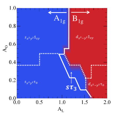
FIG. S1.: Phase diagram based on the leading pairing amplitudes given by self-consistent calculations using tight-binding parameters appropriate to single-layer FeSe. The tight-binding parameters used can be found in Ref. Yu et al. (2013). The blue shaded areas correspond to dominant pairing channels with an $s_{x^{2}y^{2}}$ form factor while the red shading covers those with a $d_{x^{2}-y^{2}}$ form factor. The continuous line separates regions where the pairing belongs to the $A_{1g}$ and the $B_{1g}$ representations respectively. The $1\times 1$ matrix in the $d_{xy}$ subspace is represented by $\boldsymbol{1}_{xy}$.

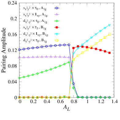
FIG. S2.: Leading pairing amplitudes (vertical axis) for a dispersion typical of alkaline iron selenides for fixed $J_{2}=1.5,A_{O}=0.3$ and varying NN-NNN ratio $A_{L}$ (horizontal axis). The $\tau$ label indicates a dominant $d_{xz},d_{yz}$ sector while $\mathbf{1}_{xy}$ marks a $d_{xy}$ dominant pairing. For $0.8\leq A_{L}\leq 0.94$ the leading pairing is in the $s\tau_{3}$ channel shown in dark filled squares. Note that the reduced parameter space for the $s\tau_{3}$ is due to the proximity to the phase boundary and for lower values of $A_{O}$ the range over which this pairing leads is increased.

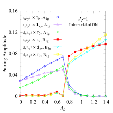
(a)

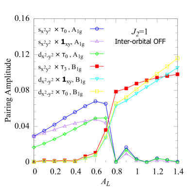
(b)

FIG. S3.: Leading intra-orbital pairing amplitudes (vertical axis) for a dispersion typical of alkaline iron selenides for fixed $J_{2}=1,A_{O}=0.2$ and varying NN-NNN ratio $A_{L}$ (horizontal axis) with (a) and without (b) inter-orbital exchange interactions. As mentioned in the discussion above, no significant changes are observed.

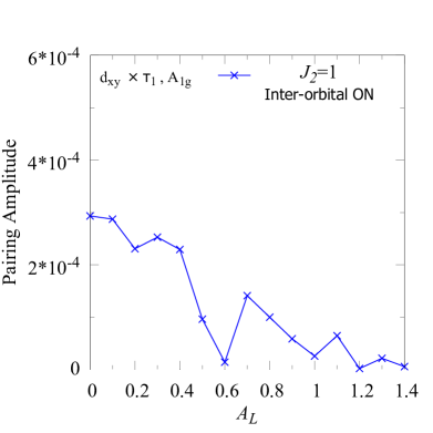
(a)

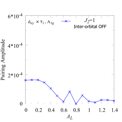
(b)

FIG. S4.: Leading inter-orbital pairing amplitude (vertical axis) for a dispersion typical of alkaline iron selenides for fixed $J_{2}=1,A_{O}=0.2$ and varying NN-NNN ratio $A_{L}$ (horizontal axis) with (a) and without (b) inter-orbital exchange interactions. As mentioned in the discussion above, no significant changes are observed.

References

- Anderson (2007) P. W. Anderson, “Is there glue in cuprate superconductors?” Science 316, 1705–1707 (2007).
- Kamihara et al. (2008) Y. Kamihara, T. Watanabe, M. Hirano, and H. Hosono, “Iron-based layered superconductor La[O1-xFx]FeAs () with K,” J. Am. Chem. Soc. 130, 3296–3297 (2008).
- Johnston (2010) D. C. Johnston, “The puzzle of high temperature superconductivity in layered iron pnictides and chalcogenides,” Adv. Phys. 59, 803–1061 (2010).
- Si et al. (2016) Q. Si, R. Yu, and E. Abrahams, “High-temperature superconductivity in iron pnictides and chalcogenides,” Nature Rev. Mater. 1, 16017 (2016).
- Wang and Lee (2011) F. Wang and D.-H. Lee, “The electron-pairing mechanism of iron-based superconductors,” Science 332, 200–204 (2011).
- Hosono and Kuroki (2015) H. Hosono and K. Kuroki, “Iron-based superconductors: Current status of materials and pairing mechanism,” Physica C 514, 399–422 (2015).
- Hirschfeld (2016) Peter J. Hirschfeld, “Using gap symmetry and structure to reveal the pairing mechanism in Fe-based superconductors,” C. R. Physique 17, 197–231 (2016).
- Qazilbash et al. (2009) M. M. Qazilbash, J. J. Hamlin, R. E. Baumbach, Lijun Zhang, M. B. Maple, and D. N. Basov, “Electronic correlations in the iron pnictides,” Nat. Phys. 5, 647–650 (2009).
- Si and Abrahams (2008) Q. Si and E. Abrahams, “Strong correlations and magnetic frustration in the high iron pnictides,” Phys. Rev. Lett. 101, 076401 (2008).
- Yin et al. (2011) Z. P. Yin, K. Haule, and G. Kotliar, “Magnetism and charge dynamics in iron pnictides,” Nat. Phys. 7, 294–297 (2011).
- Wang et al. (2012a) Q.-Y. Wang, Z. Li, W.-H. Zhang, Z.-C. Zhang, J.-S. Zhang, L. Wei, D. Hao, O. Yun-Bo, D. Peng, C. Kai, W. Jing, S. Can-Li, H. Ke, J. Jin-Feng, J. Shuai-Hua, W. Ya-Yu, W. Li-Li, C. Xi, M Xa-Cun, and X. Qi-Kun, “Interface-induced high-temperature superconductivity in single unit-cell FeSe films on SrTiO3,” Chin. Phys. Lett. 29, 037402 (2012a).
- Lee et al. (2014) J. J. Lee, F. T. Schmitt, R. G. Moore, S. Johnston, Y.-T. Cui, W. Li, M. Li, Z. K. Liu, M. Hashimoto, Y. Zhang, D. H. Lu, T. P. Devereaux, D.-H. Lee, and Z.-X. Shen, “Interfacial mode coupling as the origin of the enhancement of Tc in FeSe films on SrTiO3,” Nature 515, 245–248 (2014).
- Mou et al. (2011) D. Mou, S. Liu, X. Jia, J. He, Y. Peng, L. Zhao, L. Yu, G. Liu, S. He, and X. Dong, “Distinct fermi surface topology and nodeless superconducting gap in a (Tl0.58Rb0.42)Fe1.72Se2 superconductor,” Phys Rev Lett. 106, 107001 (2011).
- Zhang et al. (2013) C. Zhang, L. W. Harriger, Z. Yin, W. Lv, M. Wang, G. Tan, Y. Song, D. L. Abernathy, W. Tian, and T. Egami, “Measurement of a double neutron-spin resonance and an anisotropic energy gap for underdoped superconducting NaFe0.985Co0.015As using inelastic neutron scattering,” Phys. Rev. Lett. 111, 207002 (2013).
- Wang et al. (2011) X.-P. Wang, T. Qian, P. Richard, P. Zhang, J. Dong, H.-D. Wang, C.-H. Dong, M.-H. Fang, and H. Ding, “Strong nodeless pairing on separate electron Fermi surface sheets in (Tl, K)Fe1.78Se2 probed by ARPES,” Europhys. Lett. 93, 57001 (2011).
- Xu et al. (2012) M. Xu, Q. Q. Ge, R. Peng, Z. R. Ye, J. Jiang, F. Chen, X. P. Shen, B. P. Xie, Y. Zhang, A. F. Wang, X. F. Wang, X. H. Chen, and D. L. Feng, “Evidence for an s-wave superconducting gap in KxFe2-ySe2 from angle-resolved photoemission,” Phys. Rev. B 85, 220504 (2012).
- Wang et al. (2012b) X.-P. Wang, P. Richard, X. Shi, A. Roekeghem, Y.-B. Huang, E. Razzoli, T. Qian, E. Rienks, S. Thirupathaiah, H.-D. Wang, C.-H. Dong, M.-H. Fang, M. Shi, and H. Ding, “Observation of an isotropic superconducting gap at the Brillouin zone center of Tl0.63K0.37Fe1.78Se2,” Europhys. Lett. 99, 67001 (2012b).
- Park et al. (2011) J. T. Park, G. Friemel, Yuan Li, J.-H. Kim, V. Tsurkan, J. Deisenhofer, H.-A. Krug von Nidda, A. Loidl, A. Ivanov, B. Keimer, and D. S. Inosov, “Magnetic resonant mode in the low-energy spin-excitation spectrum of superconducting Rb2Fe4Se5 single crystals,” Phys. Rev. Lett. 107, 177005 (2011).
- Friemel et al. (2012) G. Friemel, J. T. Park, T. A. Maier, V. Tsurkan, Yuan Li, J. Deisenhofer, H.-A. Krug von Nidda, A. Loidl, A. Ivanov, B. Keimer, and D. S. Inosov, “Reciprocal-space structure and dispersion of the magnetic resonant mode in the superconducting phase of RbxFe2-ySe2 single crystals,” Phys. Rev. B 85, 140511(R) (2012).
- Eschrig (2006) M. Eschrig, “The effect of collective spin-1 excitations on electronic spectra in high- superconductors,” Adv. Phys. 55, 47 (2006).
- Schaibley et al. (2016) J. R. Schaibley, H. Yu, G. Clark, P. Rivera, J. S. Ross, K. L. Seyler, W. Yao, and X. Xul, “Valleytronics in 2D materials?” Nature Rev. Mater. 1, 16055 (2016).
- Yi et al. (2015) M. Yi, Z.-K. Liu, Y. Zhang, R. Yu, J. X. Zhu, J. J. Lee, R. G Moore, F. T. Schmitt, W. Li, S. C. Riggs, J.-H. Chu, B. Lv, J. Hu, M. Hashimoto, S.-K. Mo, Z. Hussain, Z. Q. Mao, C. W. Chu, I. R. Gisher, Q. Si, Z.-X. Shen, and D. H. Lu, “Observation of universal strong orbital-dependent correlation effects in iron chalcogenides,” Nat. Comm. 6, 7777 (2015).
- Yi et al. (2013) M. Yi, D. H. Lu, R. Yu, S. C. Riggs, J.-H. Chu, B. Lv, Z. K. Liu, M. Lu, Y.-T. Cui, M. Hashimoto, S.-K. Mo, Z. Hussain, C. W. Chu, I. R. Fisher, Q. Si, and Z.-X. Shen, “Observation of temperature-induced crossover to an orbital-selective Mott phase in AxFe2-ySe2 (A = K, Rb) superconductors,” Phys. Rev. Lett. 110, 067003 (2013).
- Wang et al. (2014) Zhe Wang, M. Schmidt, J. Fischer, V. Tsurkan, M. Greger, D. Vollhardt, A. Loidl, and J. Deisenhofer, “Orbital-selective metal–insulator transition and gap formation above in superconducting Rb1-xFe2-ySe2,” Nat. Comm. 5, 3202 (2014).
- Ding et al. (2014) Xiaxin Ding, Yiming Pan, Huan Yang, and Hai-Hu Wen, “Strong and nonmonotonic temperature dependence of Hall coefficient in superconducting KxFe2-ySe2,” Phys. Rev. B 89, 224515 (2014).
- Li et al. (2014) Wei Li, Chunfeng Zhang, Shenghua Liu, Xiaxin Ding, Xuewei Wu, Xiaoyong Wang, Hai-Hu Wen, and Min Xiao, “Mott behavior in KxFe2-ySe2 superconductors studied by pump-probe spectroscopy,” Phys. Rev. B 89, 134515 (2014).
- Yu et al. (2013) R. Yu, P. Goswami, Q. Si, P. Nikolic, and J.-X. Zhu, “Superconductivity at the border of electron localization and itinerancy,” Nat. Commun. 4, 2783 (2013).
- Liu et al. (2015) Z. K. Liu, M. Yi, Y. Zhang, J. Hu, R. Yu, J.-X. Zhu, R.-H. He, Y. L. Chen, M. Hashimoto, R. G. Moore, S.-K. Mo, Z. Hussain, Q. Si, Z. Q. Mao, D. H. Lu, and Z.-X. Shen, “Experimental observation of incoherent-coherent crossover and orbital-dependent band renormalization in iron chalcogenide superconductors,” Phys. Rev. B 92, 235138 (2015).
- Yu and Si (2011) R. Yu and Q. Si, “Mott transition in multiorbital models for iron pnictides,” Phys. Rev. B 84, 235115 (2011).
- Yu and Si (2013) R. Yu and Q. Si, “Orbital-selective Mott phase in multiorbital models for alkaline iron selenides K1-xFe2-ySe2,” Phys. Rev. Lett. 110, 146402 (2013).
- de’ Medici et al. (2014) L. de’ Medici, G. Giovannetti, and M. Capone, “Selective Mott physics as a key to iron superconductors,” Phys. Rev. Lett. 112, 177001 (2014).
- R.Yu et al. (2014) R.Yu, J.-X. Zhu, and Q. Si, “Orbital-selective superconductivity, gap anisotropy, and spin resonance excitations in a multiorbital model for iron pnictides,” Phys. Rev. B 89, 024509 (2014).
- Yin et al. (2014) Z. P. Yin, K. Haule, and G. Kotliar, “Spin dynamics and orbital-antiphase pairing symmetry in iron-based superconductors,” Nat. Phys. 10, 845–850 (2014).
- Ong et al. (2016) Tzen Ong, Piers Coleman, and Jörg Schmalian, “Concealed d-wave pairs in the condensate of iron-based superconductors,” Proc. Natl. Acad. Sci. U.S.A. 113, 5486–5491 (2016).
- Hao and Hu (2014) N. Hao and J. Hu, “Odd parity pairing and nodeless antiphase in iron-based superconductors,” Phys. Rev. B 89, 045144 (2014).
- Raghu et al. (2008) S. Raghu, Xiao-Liang Qi, Chao-Xing Liu, D. J. Scalapino, and Shou-Cheng Zhang, “Minimal two-band model of the superconducting iron oxypnictides,” Phys. Rev. B 77, 220503(R) (2008).
- Nica et al. (2015) E. M. Nica, R. Yu, and Q. Si, “Glide reflection symmetry, Brillouin zone folding and superconducting pairing for space group,” Phys. Rev. B 92, 174520 (2015).
- Dai (2015) P. Dai, “Antiferromagnetic order and spin dynamics in iron-based superconductors,” Rev. Mod. Phys. 87, 855–896 (2015).
- Balian and Werthamer (1963) R. Balian and N. R. Werthamer, “Superconductivity with pairs in a relative p wave,” Phys. Rev. 131, 1553–1564 (1963).
- Leggett (1975) Anthony J. Leggett, “A theoretical description of the new phase of 3He,” Rev. Mod. Phys. 47, 331–414 (1975).
- Sigrist and Ueda (1991) M. Sigrist and K. Ueda, “Phenomenological theory of unconventional superconductivity,” Rev. Mod. Phys. 63, 239–311 (1991).
- Fang et al. (2008) C. Fang, H. Yao, W.-F. Tsai, J. P. Hu, and S. A. Kivelson, “Theory of electron nematic order in LaFeAsO,” Phys. Rev. B 77, 224509 (2008).
- Xu et al. (2008) C. Xu, M. Müller, and S. Sachdev, “Ising and spin orders in the iron-based superconductors,” Phys. Rev. B 78, 020501(R) (2008).
- Seo et al. (2008) K. Seo, B. Andrei Bernevig, and J. Hu, “Pairing symmetry in a two-orbital exchange coupling model of oxypnictides,” Phys. Rev. Lett. 101, 206404 (2008).
- Moreo et al. (2009) A. Moreo, M. Daghofer, J. A. Riera, and E. Dagotto, “Properties of a two-orbital model for oxypnictide superconductors: Magnetic order, spin-singlet pairing channel, and its nodal structure,” Phys. Rev. B 79, 134502 (2009).
- Chen et al. (2009) W.-Q. Chen, K.-Y. Yang, Y. Zhou, and F.-C. Zhang, “Strong coupling theory for superconducting iron pnictides,” Phys. Rev. Lett. 102, 047006 (2009).
- Yang et al. (2013) F. Yang, F. Wang, and D.-H. Lee, “Fermiology, orbital order, orbital fluctuations, and Cooper pairing in iron-based superconductors,” Phys. Rev. B 88, 100504(R) (2013).
- Berg et al. (2009) E. Berg, S. A. Kivelson, and D. J. Scalapino, “A twisted ladder: relating the Fe superconductors to the high- cuprates,” New J. Phys. 11, 085007 (2009).
- Lv et al. (2010) W. Lv, F. Krüger, and P. Phillips, “Orbital ordering and unfrustrated (,0) magnetism from degenerate double exchange in the iron pnictides,” Phys. Rev. B 82, 045125 (2010).
- Bascones et al. (2012) E. Bascones, B. Valenzuela, and M. J. Calderón, “Orbital differentiation and the role of orbital ordering in the magnetic state of fe superconductors,” Phys. Rev. B 86, 174508 (2012).
- Graser et al. (2009) S. Graser, T. A. Maier, P. J. Hirschfeld, and D. J. Scalapino, “Near-degeneracy of several pairing channels in multiorbital models for the Fe pnictides,” New J. Phys. 11, 025016 (2009).
- Goswami et al. (2010) P. Goswami, P. Nikolic, and Q. Si, “Superconductivity in multi-orbital model and its implications for iron pnictides,” Europhys. Lett. 91, 37006 (2010).
- Zhang et al. (2011) Y. Zhang, L. X. Yang, M. Xu, Z. R. Ye, F. Chen, C. He, H. C. Xu, J. Jiang, B. P. Xie, J. J. Ying, X. F. Wang, X. H. Chen, J. P. Hu, M. Matsunani, S. Kimura, and D. L. Feng, “Nodeless superconducting gap in AxFe2Se2(A=K, Cs) revealed by angle-resolved photoemission spectroscopy,” Nat. Mater. 10, 273–277 (2011).
- Liu et al. (2012) Z.-H. Liu, P. Richard, N. Xu, G. Xu, Y. Li, X.-C. Fang, L.-L. Jia, and et al, “Three dimensionality and orbital characters of the Fermi surface in (Tl, Rb)yFe2-xSe2,” Phys. Rev. Lett. 109, 037003 (2012).
- Kittaka et al. (2014) S. Kittaka, Y. Aoki, Y. Shimura, T. Sakakibara, S. Seiro, and et al, “Multiband superconductivity in unexpected deficiency of nodal quasiparticles in CeCu2Si2,” Phys. Rev. Lett. 112, 067002 (2014).

REFERENCES

- Raghu et al. (2008) S. Raghu, Xiao-Liang Qi, Chao-Xing Liu, D. J. Scalapino, and Shou-Cheng Zhang, “Minimal two-band model of the superconducting iron oxypnictides,” Phys. Rev. B 77, 220503(R) (2008).
- Sigrist and Ueda (1991) M. Sigrist and K. Ueda, “Phenomenological theory of unconventional superconductivity,” Rev. Mod. Phys. 63, 239–311 (1991).
- Nica et al. (2015) E. M. Nica, R. Yu, and Q. Si, “Glide reflection symmetry, Brillouin zone folding and superconducting pairing for space group,” Phys. Rev. B 92, 174520 (2015).
- Yu and Si (2013) R. Yu and Q. Si, “Orbital-selective Mott phase in multiorbital models for alkaline iron selenides K1-xFe2-ySe2,” Phys. Rev. Lett. 110, 146402 (2013).
- Yu et al. (2013) R. Yu, P. Goswami, Q. Si, P. Nikolic, and J.-X. Zhu, “Superconductivity at the border of electron localization and itinerancy,” Nat. Commun. 4, 2783 (2013).
- R.Yu et al. (2014) R.Yu, J.-X. Zhu, and Q. Si, “Orbital-selective superconductivity, gap anisotropy, and spin resonance excitations in a multiorbital model for iron pnictides,” Phys. Rev. B 89, 024509 (2014).
- Eschrig (2006) M. Eschrig, “The effect of collective spin-1 excitations on electronic spectra in high- superconductors,” Adv. Phys. 55, 47 (2006).
- Fong et al. (1995) H. F. Fong, B. Keimer, P. W. Anderson, D. Reznik, F. Doğan, and I. A. Aksay, “Phonon and magnetic neutron scattering at 41 mev in YBa2Cu3O7,” Phys. Rev. Lett. 75, 316 (1995).
- Yi et al. (2015) M. Yi, Z.-K. Liu, Y. Zhang, R. Yu, J. X. Zhu, J. J. Lee, R. G Moore, F. T. Schmitt, W. Li, S. C. Riggs, J.-H. Chu, B. Lv, J. Hu, M. Hashimoto, S.-K. Mo, Z. Hussain, Z. Q. Mao, C. W. Chu, I. R. Gisher, Q. Si, Z.-X. Shen, and D. H. Lu, “Observation of universal strong orbital-dependent correlation effects in iron chalcogenides,” Nat. Comm. 6, 7777 (2015).