Historic behaviour for nonautonomous contraction mappings

Abstract.

We consider a parametrised perturbation of a $\mathscr{C}^{r}$ diffeomorphism on a closed smooth Riemannian manifold with $r\geq 1$, modeled by nonautonomous dynamical systems. A point without time averages for a (nonautonomous) dynamical system is said to have historic behaviour. It is known that for any $\mathscr{C}^{r}$ diffeomorphism, the observability of historic behaviour, in the sense of the existence of a positive Lebesgue measure set consisting of points with historic behaviour, disappears under absolutely continuous, independent and identically distributed (i.i.d.) noise. On contrast, we show that the observability of historic behaviour can appear by a non-i.i.d. noise: we consider a contraction mapping for which the set of points with historic behaviour is of zero Lebesgue measure and provide an absolutely continuous, non-i.i.d. noise under which the set of points with historic behaviour is of positive Lebesgue measure.

1. Introduction

This paper concerns nonautonomous dynamical systems on a parametrised family of $\mathscr{C}^{r}$ diffeomorphisms on a closed smooth Riemannian manifold $M$ with $r\geq 1$. Given a mapping $\theta:\Omega\to\Omega$ on base set $\Omega$, a nonautonomous dynamical system (abbreviated NDS henceforth) on $M$ over $\theta$ is given as a mapping $F:\mathbb{N}_{0}\times\Omega\times M\to M$ satisfying $F(0,\omega,\cdot)=\mathrm{id}_{M}$ for each $\omega\in\Omega$ and the cocycle property

$$F(n+m,\omega,x)=F(n,\theta^{m}\omega,F(m,\omega,x)),\quad n,m\in\mathbb{N}_{0},\quad\omega\in\Omega,\quad x\in M.$$

Here $\theta\omega$ denotes the value $\theta(\omega)$, and $\theta$ is called a driving system. The notation of nonautonomous dynamical systems has emerged as an abstraction of random dynamical systems (see Remark 2 for the precise definition of random dynamical systems; a standard reference is the monograph by Arnold [4], see also [6, 8] for representation of Markov chains of random perturbations by random maps). For general properties of NDS, we refer to Kloeden and Rasmussen [9]. Here it is merely stated that if we denote $F(n,\omega,\cdot)$ and $F(1,\omega,\cdot)$ by $f^{(n)}_{\omega}$ and $f_{\omega}$, respectively, then we have

(1.1) $$F(n,\omega,\cdot)\equiv f^{(n)}_{\omega}=f_{\theta^{n-1}\omega}\circ f_{\theta^{n-2}\omega}\circ\cdots\circ f_{\omega}.$$

Conversely, it is straightforward to see that given a mapping $f:\Omega\times M\to M$: $(\omega,x)\mapsto f_{\omega}(x)$, a mapping $F:\mathbb{N}_{0}\times\Omega\times M\to M$ defined by (1.1) is an NDS over $\theta$. We call it the NDS induced by $f$ over $\theta$.

A naive expectation from (1.1) is that once we impose an appropriate condition on $\omega\mapsto f_{\omega}$, the statistical properties of the driving system $\theta$ (with respect to a given probability measure $\mathbb{P}$ on $\Omega$) will be transmitted to those of $\{f^{(n)}_{\omega}\}_{n\geq 0}$ ($\mathbb{P}$-almost surely). A celebrated result in the direction is established by Araújo [1] for historic behaviour in the i.i.d. case, which inspires the work in this paper. (For another result in the direction from the viewpoint of mixing property or limit theorems, refer to [12, 14, 2] and the references therein.) To state his and our result, we define historic behaviour for $F$.

Definition 1.

For given $\omega\in\Omega$, we say that the forward orbit of $x\in M$ at $\omega$ has historic behaviour if there exists a continuous function $\varphi:M\to\mathbb{R}$ for which the time average

(1.2) $$\lim_{n\to\infty}\frac{1}{n}\sum_{j=0}^{n-1}\varphi(f^{(j)}_{\omega}(x))$$

does not exist. For short, we call $x$ a point with historic behaviour at $\omega$.

The concept of historic behaviour was introduced by Ruelle [16] for autonomous dynamical systems: Let $f_{0}:M\to M$ be a $\mathscr{C}^{r}$ diffeomorphism on $M$ and $f_{0}^{n}$ the usual $n$-th iteration of $f_{0}$ with $n\geq 0$. Then, $\mathbb{N}_{0}\times M\ni(n,x)\mapsto f_{0}^{n}(x)$ is an (autonomous) dynamical system, and a point $x\in M$ is said to have historic behaviour if there exists a continuous function $\varphi:M\to\mathbb{R}$ for which the time average $\lim_{n\to\infty}\frac{1}{n}\sum_{j=0}^{n-1}\varphi(f_{0}^{j}(x))$ does not exist. Since several statistical quantities are given as the time average of some function $\varphi$, it is natural to investigate the observability of historic behaviour in the sense of the existence of a positive Lebesgue measure set consisting of point with historic behaviour. In the autonomous situation, Bowen’s famous folklore example [17] tells that there is a $\mathscr{C}^{\infty}$ diffeomorphism on a compact surface for which the set of points with historic behaviour is of positive Lebesgue measure. However, his example was not stable under small perturbations. Hence, Takens asked in [18] whether there is a persistent class of $\mathscr{C}^{r}$ diffeomorphisms for which the set of points with historic behaviour is of positive Lebesgue measure (called Takens’ Last Problem): Very recently it was affirmatively answered by the first and third authors in [10], that will be briefly restated (in a slightly stronger form) in Theorem C. Furthermore, this was applied to detect a persistent class of 3-dimensional flows having a positive Lebesgue measure set consisting of points with historic behaviour in [11]. The reader is asked to see [17, 16, 18, 6] for the background of historic behaviour in the autonomous situation.

In the nonautonomous situation, the first result about historic behaviour was obtained by Araújo for parametrised perturbations of $\mathscr{C}^{r}$ diffeomorphisms under i.i.d. noise: if a parametrised perturbation of a $\mathscr{C}^{r}$ diffeomorphism $f_{0}$ given as an i.i.d. NDS $F$ is absolutely continuous, then the set of points with historic behaviour is a zero Lebesgue measure set (see Appendix A for the definition of absolute continuous i.i.d. NDS’s and the precise statement of Araújo’s theorem). We can choose the unperturbed system $f_{0}$ as a $\mathscr{C}^{r}$ diffeomorphism for which the set of points with historic behaviour is persistently of positive Lebesgue measure, that means the disappearance of historic behaviour under i.i.d. noise (although the existence of a residual set consisting of points with historic behaviour for expanding maps is preserved under any random perturbations, refer to [13]). Our purpose in this paper is to show the appearance of historic behaviour under some “historic” noise.

1.1. Setting and result

Let $M$ be the circle given by $M=\mathbb{R}/\mathbb{Z}$. We endow $M$ with a metric $d_{M}(\cdot,\cdot)$, where $d_{M}(x,y)$ is the infimum of $|\tilde{x}-\tilde{y}|$ over all representatives $\tilde{x},\tilde{y}$ of $x,y\in M$, respectively. Let $\pi_{M}:\mathbb{R}\to M$ be the canonical projection on the circle, i.e., $\pi_{M}(\tilde{x})$ is the equivalent class of $\tilde{x}\in\mathbb{R}$. We write $I_{0}$ for $\pi_{M}\left([\frac{1}{4},\frac{3}{4}]\right)$. Let $f_{0}$ be a $\mathscr{C}^{r}$ diffeomorphism on $M$ such that

(1.3) $$f_{0}(x)=\frac{1}{2}x+\frac{1}{4}\mod 1,\quad x\in I_{0},$$

and that $\inf_{x\in M}Df_{0}(x)>0$ (see Figure 2). We also assume that $f_{0}$ has exactly one source. Then, it is not difficult to see that the set of points with historic behaviour for $f_{0}$ is an empty set, in particular, a zero Lebesgue measure set. (Note that basin of attraction of $\pi_{M}(\frac{1}{2})$ is the whole space $M$ except the source.)

Next we introduce our main hypothesis for driving systems. Let $\Omega$ be a metric space equipped with the Borel $\sigma$-field, and $\mathbb{P}$ a probability measure on $\Omega$. Let $\theta:\Omega\to\Omega$ be a continuous mapping. Given an integer $\nu\geq 0$, $\omega\in\Omega$ and an open set $U\subset\Omega$, we say that an integer $j$ is in a $\nu$-trapped period of $\omega$ for $U$ if $j\geq\nu$ and $\theta^{j-i}\omega\in U$ for all $i\in[0,\nu]$. For $n\geq 1$, we set

$$N_{\nu}(\omega,U;n)=\#\{j\in[0,n-1]\;:\;\text{$j$ is in a $\nu$-trapped period of $\omega$ for $U$}\}.$$

Let $U_{\delta}(\omega)$ be the ball of $\omega\in\Omega$ with radius $\delta>0$. We will assume the following condition:

• There is a $\mathbb{P}$-positive measure set $\Gamma\subset\Omega$ and distinct points $p$ and $\hat{p}$ such that for any integer $\nu\geq 0$ and positive number $\delta$, one can find two distinct real numbers $\lambda_{1}$ and $\lambda_{2}$ in $[0,1]$ and subsequences $\{n_{1}(J)\}_{J\geq 1}$ and $\{n_{2}(J)\}_{J\geq 1}$ of $\mathbb{N}$ such that

  $$\lim_{J\to\infty}\frac{N_{\nu}(\omega,U_{\delta}(p);n_{i}(J))}{n_{i}(J)}=1-\lambda_{i},\quad\lim_{J\to\infty}\frac{N_{\nu}(\omega,U_{\delta}(\hat{p});n_{i}(J))}{n_{i}(J)}=\lambda_{i}$$

  for $i=1,2$.

Let $\kappa:\Omega\to[-1,1]$ be a surjective continuous function such that $\kappa(p)\neq\kappa(\hat{p})$ and that the pushforward $\kappa_{*}\mathbb{P}$ of $\mathbb{P}$ by $\kappa$ is absolutely continuous with respect to $\mathrm{Leb}_{\mathbb{R}}$. Fix a noise level $0<\epsilon<\frac{1}{8}$. We define a parametrised perturbation $f:\Omega\times M\to M$ of $f_{0}$ by

(1.4) $$f_{\omega}(x)\equiv f(\omega,x)=f_{0}(x)+\epsilon\kappa(\omega)\mod 1,\quad(\omega,x)\in\Omega\times M.$$

Now we can provide our main theorems:

Theorem A.

Suppose that $\theta$ satisfies the condition (H). Let $F$ be the NDS induced by $f$ in (1.4) over $\theta$. Then for any $\omega\in\Gamma$, there exists a positive Lebesgue measure set (including $I_{0}$) consisting of points with historic behaviour at $\omega$.

For an application of Theorem A, we will show that the condition (H) can be satisfied by the classical Bowen example. Let $\Omega$ be a compact surface and $\mathbb{P}$ the normalised Lebesgue measure of $\Omega$.

Theorem B.

The time-one map $\theta$ of the Bowen flow (definition given in Subsection 2.2) on $\Omega$ satisfies the condition (H).

We will also show that the persistent driving systems in [10] satisfy the condition (H). Let $\mathrm{Diff}^{\tilde{r}}(\Omega,\Omega)$ be the set of all $\mathscr{C}^{\tilde{r}}$ diffeomorphisms on $\Omega$ endowed with the usual $\mathscr{C}^{\tilde{r}}$ metric with $2\leq\tilde{r}<\infty$, and let $\mathcal{N}\subset\mathrm{Diff}^{\tilde{r}}(\Omega,\Omega)$ be a Newhouse open set.

Theorem C.

There exists a dense subset $\mathcal{D}$ of $\mathcal{N}$ such that all $\theta\in\mathcal{D}$ satisfies the condition (H).

1.2. Problem

Before starting the proofs of main theorems, we briefly consider historic behaviour for nonautonomous contraction mappings in more general setting. Let $f_{0}$ be as in (1.3). Let $(\Omega,\mathcal{F},\mathbb{P})$ be a probability space. Let $\kappa$ be a measurable function on $\Omega$ with values in $[-1,1]$ $\mathbb{P}$-almost surely. We define $f:\Omega\times M\to M$ by

(1.5) $$f_{\omega}(x)\equiv f(\omega,x)=f_{0}(x)+\epsilon\kappa(\omega),\quad(\omega,x)\in\Omega\times M.$$

Furthermore, we assume that $\theta$ is nonsingular with respect to $\mathbb{P}$ (i.e., $\mathbb{P}(\theta^{-1}\Gamma)=1$ if $\Gamma$ is measurable and $\mathbb{P}(\Gamma)=1$).

We say that the driving system $\theta$ is historic if there exists a positive measure set $\Gamma$ with respect to $\mathbb{P}$ such that for each $\omega\in\Gamma$, one can find an integrable function $b:\Omega\to\mathbb{R}$ whose time average $\lim_{n\to\infty}\frac{1}{n}\sum_{j=0}^{n-1}b(\theta^{j}\omega)$ does not exist. Otherwise, we say that $\theta$ is non-historic.

Remark 2.

A measurable NDS $F$ over a measurable driving system $\theta$ is said to be a random dynamical system (abbreviated RDS) if $\theta$ is measure-preserving (refer to [4]; important examples of random dynamical systems are i.i.d. NDS’s, see Appendix A). It follows from Birkhoff’s ergodic theorem that any measure-preserving driving system is non-historic. That is, any random dynamical system is an NDS over a non-historic driving system. See Figure 1.

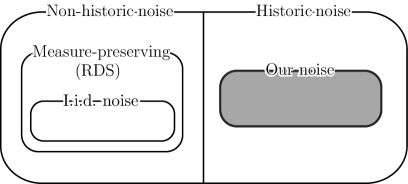
Figure 1. Classification of nonautonomous dynamical systems.

The following proposition can be shown by a standard graph-transformation argument, but might be suggestive for historic behaviour of nonautonomous contraction mappings. See Appendix B for the proof.

Proposition 3.

Let $\theta$ be measurably invertible. Let $f$ be as in (1.5) and $F$ the NDS induced by $f$ over a driving system $\theta$. Suppose that $\theta$ is non-historic. Then for $\mathbb{P}$-almost every $\omega$, the set of points in $I_{0}$ with historic behaviour at $\omega$ is an empty set, in particular, a Lebesgue zero measure set.

Comparing Theorem A with proposition 3, one may naturally ask the following problem.

Problem 4.

Let $f$ be as in (1.5) and $F$ the NDS induced by $f$ over a driving system $\theta$. Suppose that $\theta$ is historic. Then under some mild condition on $\kappa$, can one find a positive measure set $\Gamma$ with respect to $\mathbb{P}$ such that there exists a positive Lebesgue measure set (including $I_{0}$) consisting of points with historic behaviour at $\omega$ for any $\omega\in\Gamma$?

Remark 5.

Apart from driving systems, one can consider generalisations of Theorem A to other unperturbed systems $f_{0}$: It is highly likely that the existence of a positive Lebesgue measure set consisting of points with historic behaviour remains true for any $\mathscr{C}^{r}$ diffeomorphism on any closed smooth Riemannian manifold $M$, only by requiring that $f_{0}$ has a sink (with an appropriate modification on the formulation of small perturbation $f$ in higher dimension; see Example 2 in [1]). It might also be possible (and of great interest) to explore generalisation to hyperbolic mappings $f_{0}$ by considering their transfer operators, refer to [5]. However, in order to keep our presentation as transparent as possible, we restricted ourselves to the concrete example given in (1.3).

2. Proofs

2.1. Proof of Theorem A

We start the proof of Theorem A by noting that $f_{\omega}(I_{0})\subset I_{0}$ and $f_{\omega}|_{I_{0}}:I_{0}\to I_{0}$ has a unique fixed point, denoted by $X_{\omega}$, for each $\omega\in\Omega$. In particular, for $\omega=p,\hat{p}$,

(2.1) $$X_{p}=\frac{1}{2}+2\epsilon\kappa(p),\quad X_{\hat{p}}=\frac{1}{2}+2\epsilon\kappa(\hat{p}).$$

See Figure 2.

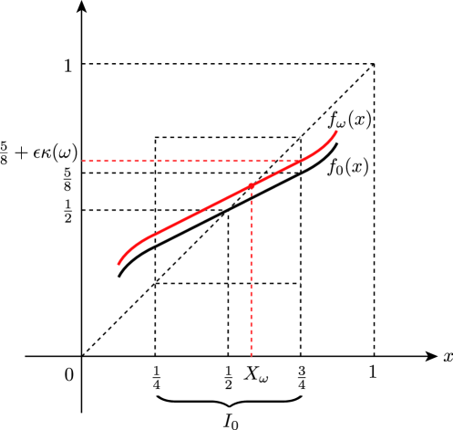
Figure 2. Locally contraction mappings $f_{0}$ and $f_{\omega}$.

We need the following elementary lemma.

Lemma 6.

For any $n\in\mathbb{N}_{0}$, $x\in I_{0}$ and $\omega,\omega^{\prime}\in\Omega$, we have

(2.2) $$d_{M}\left(f^{(n)}_{\omega}(x),X_{\omega^{\prime}}\right)\leq\frac{1}{2^{n}}+6\epsilon\max_{0\leq j\leq n-1}\left|\kappa(\theta^{j}\omega)-\kappa(\omega^{\prime})\right|.$$

Proof.

Fix $n\in\mathbb{N}_{0}$, $x\in I_{0}$ and $\omega,\omega^{\prime}\in\Omega$. Noting that $X_{\omega^{\prime}}=\pi_{M}(\frac{1}{2}+2\epsilon\kappa(\omega^{\prime}))$ together with (1.1), we have

$$d_{M}\left(f^{(n)}_{\omega}(x),X_{\omega^{\prime}}\right) \leq d_{M}\left(f_{\theta^{n-1}\omega}(f^{(n-1)}_{\omega}(x)),f_{\theta^{n-1}\omega}(X_{\theta^{n-1}\omega})\right)+d_{M}\left(X_{\theta^{n-1}\omega},X_{\omega^{\prime}}\right)$$

$$\leq\frac{1}{2}d_{M}\left(f^{(n-1)}_{\omega}(x),X_{\theta^{n-1}\omega}\right)+2\epsilon\left|\kappa(\theta^{n-1}\omega)-\kappa(\omega^{\prime})\right|.$$

Reiterating this argument, we finally get that $d_{M}\left(f^{(n)}_{\omega}(x),X_{\omega^{\prime}}\right)$ is bounded by

$$\frac{1}{2^{n}}d_{M}\left(x,X_{\omega}\right)+2\epsilon\left(\sum_{j=1}^{n-1}\frac{|\kappa(\theta^{n-j-1}\omega)-\kappa(\theta^{n-j}\omega)|}{2^{j}}+\left|\kappa(\theta^{n-1}\omega)-\kappa(\omega^{\prime})\right|\right).$$

Hence, the conclusion follows from the triangle inequality

$$|\kappa(\theta^{n-j-1}\omega)-\kappa(\theta^{n-j}\omega)|\leq|\kappa(\theta^{n-j-1}\omega)-\kappa(\omega^{\prime})|+|\kappa(\omega^{\prime})-\kappa(\theta^{n-j}\omega)|.$$

This completes the proof. ∎

We continue the proof of Theorem A. We let $V(X_{p})$ and $V(X_{\hat{p}})$ be the $\rho_{0}$-neighbourhoods of $X_{p}$, $X_{\hat{p}}$ in $M$, respectively, with $\rho_{0}=\frac{\epsilon|\kappa(p)-\kappa(\hat{p})|}{2}$. By (2.1), $V(X_{p})\cap V(X_{\hat{p}})=\emptyset$. Fix a positive integer $\nu_{0}$ satisfying

(2.3) $$\frac{1}{2^{\nu_{0}}}\leq\frac{\rho_{0}}{3}.$$

Furthermore, we let $\delta_{0}^{\prime}$ be a positive number such that $d_{\Omega}(\omega,p_{1})<\delta_{0}^{\prime}$ implies $|\kappa(\omega)-\kappa(p_{1})|\leq\frac{\rho_{0}}{18}$ with $p_{1}=p$ and $\hat{p}$, and set

(2.4) $$\delta_{0}=\min\left\{\delta_{0}^{\prime},\frac{\mathrm{dist}_{\Omega}(p,\partial\Omega)}{2},\frac{\mathrm{dist}_{\Omega}(\hat{p},\partial\Omega)}{2}\right\},$$

so that $U_{\delta_{0}}(p)\cap U_{\delta_{0}}(\hat{p})=\emptyset$ and $(U_{\delta_{0}}(p)\cup U_{\delta_{0}}(\hat{p}))\cap\partial\Omega=\emptyset$.

Let $j$ be in a $\nu_{0}$-trapped period of $\omega\in\Omega$ for $U_{\delta_{0}}(p)$. Then, we have

(2.5) $$\max_{0\leq i\leq\nu_{0}}d_{\Omega}(\theta^{j-i}\omega,p)\leq\delta_{0}.$$

On the other hand, applying (2.2) with $n,x,\omega$ and $\omega^{\prime}$ replaced by $\nu_{0}$, $f^{(j-\nu_{0})}_{\omega}(x)$, $\theta^{j-\nu_{0}}\omega$ and $p$ together with (1.1), we have

$$d_{M}(f_{\omega}^{(j)}(x),X_{p})\leq\frac{1}{2^{\nu_{0}}}+6\epsilon\max_{0\leq i\leq\nu_{0}}\left|\kappa(\theta^{j-i}\omega)-\kappa(p)\right|$$

for all $x\in I_{0}$. Therefore, it follows from (2.3), (2.4) and (2.5) that

$$d_{M}(f_{\omega}^{(j)}(x),X_{p})\leq\frac{2}{3}\rho_{0},$$

that is, $f_{\omega}^{(j)}(x)\in V(X_{p})$. A similar argument implies that if $j$ is in a $\nu_{0}$-trapped period of $\omega\in\Omega$ for $U_{\delta_{0}}(\hat{p})$, then $f_{\omega}^{(j)}(x)\in V(X_{\hat{p}})$ for any $x\in I_{0}$.

We assume that $\lambda_{1}<\lambda_{2}$ without loss of generality. Let $\varphi_{0}:M\to[0,1]\subset\mathbb{R}$ be a nonnegative-valued continuous function such that $\varphi_{0}(x)=1$ if $x$ is in $V(X_{p})$ and $\varphi_{0}(x)=0$ if $x$ is in $V(X_{\hat{p}})$. For each $x\in I_{0}$ and $\omega\in\Gamma$, by the condition (H) together with observation in the previous paragraph, we have

$$\frac{1}{n_{1}(J)}\sum_{j=0}^{n_{1}(J)}\varphi_{0}(f_{\omega}^{(j)}(x))\geq\frac{\#\{0\leq j\leq n_{1}(J)\mid f^{(j)}_{\omega}(x)\in V(X_{p})\}}{n_{1}(J)}\to 1-\lambda_{1}$$

and

$$\frac{1}{n_{2}(J)}\sum_{j=0}^{n_{2}(J)}\varphi_{0}(f_{\omega}^{(j)}(x))\leq 1-\frac{\#\{0\leq j\leq n_{2}(J)\mid f^{(j)}_{\omega}(x)\in V(X_{\hat{p}})\}}{n_{2}(J)}\to 1-\lambda_{2}$$

as $J\to\infty$. Therefore, we get

$$\liminf_{n\to\infty}\frac{1}{n}\sum^{n}_{j=0}\varphi_{0}(f_{\omega}^{(j)}(x))\leq 1-\lambda_{2}<1-\lambda_{1}\leq\limsup_{n\to\infty}\frac{1}{n}\sum^{n}_{j=0}\varphi_{0}(f_{\omega}^{(j)}(x))$$

for all $(\omega,x)$ in $\Gamma\times I_{0}$. This completes the proof of Theorem A.

2.2. Proof of Theorem B

It is mentioned in [17] that Bowen considered a surface flow $\{\theta^{t}\}_{t\in\mathbb{R}}$ generated by a smooth (at least $\mathscr{C}^{3}$) vector field with two saddle points $p$ and $\hat{p}$ and two heteroclinic orbits $\gamma$ and $\hat{\gamma}$ connecting the points, which are included in the unstable and stable manifolds of $p$ respectively, such that the closed curve $\gamma:=p\sqcup\hat{p}\sqcup\gamma\sqcup\hat{\gamma}$ is attracting in the following sense: if we denote the expanding and contracting eigenvalues of the linearised vector field around $p$ by $\alpha_{+}$ and $-\alpha_{-}$, and the ones around $\hat{p}$ by $\beta_{+}$ and $-\beta_{-}$, then $\alpha_{-}\beta_{-}>\alpha_{+}\beta_{+}$. Let $\Gamma$ be the intersection of the basin of attraction of $\gamma$ and the open set surrounded by $\gamma$, which is a nonempty open set of $\Omega$. Furthermore, we take sections $\Sigma$ and $\hat{\Sigma}$ transversally intersecting $\gamma$ and $\hat{\gamma}$, respectively. See Figure 3 for configuration.

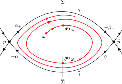
Figure 3. The Bowen flow.

Fix $\omega\in\Gamma$. Let $\{t_{j}\}_{j\geq 1}$ be successive times at which the forward orbit of $\omega$ by $\{\theta^{t}\}_{t\in\mathbb{R}}$ intersects $\Sigma$ and $\hat{\Sigma}$. By taking the sections smaller, one can assume that $\theta^{t_{j}}\omega\in\Sigma$ if $j$ is odd and $\theta^{t_{j}}\omega\in\hat{\Sigma}$ if $j$ is even. Let $T^{(p)}_{j}=t_{2j+1}-t_{2j}$ and $T^{(\hat{p})}_{j}=t_{2j}-t_{2j-1}$. It was shown in [17] that

(2.6) $$\lim_{j\to\infty}\frac{T^{(p)}_{j}}{T^{(\hat{p})}_{j}}=\sigma_{1},\quad\lim_{j\to\infty}\frac{T^{(\hat{p})}_{j+1}}{T^{(p)}_{j}}=\sigma_{2}$$

with $\sigma_{1}=\frac{\beta_{-}}{\alpha_{+}}$ and $\sigma_{2}=\frac{\alpha_{-}}{\beta_{+}}$, and

(2.7) $$\lim_{j\to\infty}\frac{T^{(p)}_{\delta,j}}{T^{(p)}_{j}}=\lim_{j\to\infty}\frac{T^{(\hat{p})}_{\delta,j}}{T^{(\hat{p})}_{j}}=1$$

for each $\delta>0$, where $T^{(p)}_{\delta,j}$ and $T^{(\hat{p})}_{\delta,j}$ are the lengths of $\{t_{2j}\leq t\leq t_{2j+1}\mid\theta^{t}\omega\in U_{\delta}(p)\}$ and $\{t_{2j-1}\leq t\leq t_{2j}\mid\theta^{t}\omega\in U_{\delta}(\hat{p})\}$, respectively, when the lengths are well-defined (in particular, for each sufficiently large $j$).

Let $n_{1}(J)=[\hat{T}_{2J-1}]$ and $n_{2}(J)=[\hat{T}_{2J}]$ with the notation $[t]$ for the integer part of $t\in\mathbb{R}$. Given $\delta>0$ and $\nu\geq 0$, let $J_{0}$ be an integer such that $\min\{T_{\delta,J_{0}}^{(p)},T_{\delta,J_{0}}^{(\hat{p})}\}\geq\nu+2$. Then, for any $J\geq J^{\prime}\geq J_{0}$, we have

$$\frac{N_{\nu}(\omega,U_{\delta}(p);n_{1}(J))}{n_{1}(J)} \geq\frac{\sum_{j=J^{\prime}}^{J}(T_{\delta,j}^{(p)}-2-\nu)}{\sum_{j=1}^{J}(T_{j}^{(p)}+T_{j}^{(\hat{p})})}$$

$$=(1-Z_{1})\cdot\frac{\sum_{j=J^{\prime}}^{J}T_{\delta,j}^{(p)}}{\sum_{j=J^{\prime}}^{J}(T_{j}^{(p)}+T_{j}^{(\hat{p})})}-Z_{2},$$

where $Z_{1}=\sum_{j=1}^{J^{\prime}-1}(T_{j}^{(p)}+T^{(\hat{p})}_{j})/\sum_{j=1}^{J}(T_{j}^{(p)}+T^{(\hat{p})}_{j})$ and $Z_{2}=(2+\nu)/\sum_{j=1}^{J}(T_{j}^{(p)}+T^{(\hat{p})}_{j})$, both of which go to $0$ as $J\to\infty$ for any fixed $J^{\prime}$. Hence, by (2.6) and (2.7), it is straightforward to see that for any $\tilde{\epsilon}>0$, there is an integer $J_{\tilde{\epsilon}}\geq J_{0}$ such that for each $J\geq J_{\tilde{\epsilon}}$,

$$\frac{N_{\nu}(\omega,U_{\delta}(p);n_{1}(J))}{n_{1}(J)}\geq(1-\tilde{\epsilon})\cdot\frac{(\sigma_{1}-\tilde{\epsilon})T_{J}^{(\hat{p})}\sum_{j=0}^{J-J_{\tilde{\epsilon}}}\{(\sigma_{1}-\tilde{\epsilon})(\sigma_{2}-\tilde{\epsilon})\}^{-j}}{(1+(\sigma_{1}+\tilde{\epsilon}))T_{J}^{(\hat{p})}\sum_{j=0}^{J-J_{\tilde{\epsilon}}}\{(\sigma_{1}+\tilde{\epsilon})(\sigma_{2}+\tilde{\epsilon})\}^{-j}}-\tilde{\epsilon}.$$

Since $\tilde{\epsilon}$ is arbitrary, we have

$$\liminf_{J\to\infty}\frac{N_{\nu}(\omega,U_{\delta}(p);n_{1}(J))}{n_{1}(J)}\geq\frac{\sigma_{1}}{1+\sigma_{1}}.$$

In a similar manner we can show that

$$\liminf_{J\to\infty}\frac{N_{\nu}(\omega,U_{\delta}(\hat{p});n_{1}(J))}{n_{1}(J)}\geq\frac{1}{1+\sigma_{1}}.$$

and that

$$\liminf_{J\to\infty}\frac{N_{\nu}(\omega,U_{\delta}(p);n_{2}(J))}{n_{2}(J)}\geq\frac{1}{1+\sigma_{2}},\quad\liminf_{J\to\infty}\frac{N_{\nu}(\omega,U_{\delta}(\hat{p});n_{2}(J))}{n_{2}(J)}\geq\frac{\sigma_{2}}{1+\sigma_{2}}.$$

This completes the proof of Theorem B with $\lambda_{1}=\frac{1}{1+\sigma_{1}}$ and $\lambda_{2}=\frac{\sigma_{2}}{1+\sigma_{2}}$.

2.3. Proof of Theorem C

In [10], we have actually shown that, for sufficiently large positive integers $z_{0}$, $n_{0}$, $k_{0}$, there exists an element $\theta=\theta_{\boldsymbol{z}}$ in any small neighbourhood of any $\mathscr{C}^{\tilde{r}}$ diffeomorphism in the Newhouse open set $\mathcal{N}$ associated with any sequence $\boldsymbol{z}=\{z_{k}\}_{k=k_{0}}^{\infty}$ of integers each entry of which is either $z_{0}$ or $z_{0}+1$ and there exists a sequence $\{R_{k}\}_{k=k_{0}}^{\infty}$ of mutually disjoint rectangles in $\Omega$ with $\mathrm{Int}R_{k_{0}}=\Gamma$ and satisfying the following conditions.

1. $\lim_{k\to\infty}\mathrm{diam}\,(R_{k})=0$.

2. There are sequences $\{a_{k}\}_{k=k_{0}}^{\infty}$, $\{b_{k}\}_{k=k_{0}}^{\infty}$ of positive integers with

   $$\limsup_{k\to\infty}\dfrac{a_{k}}{k}<\infty\quad\text{and}\quad\limsup_{k\to\infty}\dfrac{b_{k}}{k}<\infty$$

   and such that, for any $\delta>0$ and $\omega\color[rgb]{0,0,0}\in R_{k}$ with sufficiently large $k\geq k_{0}$,

   • $\theta^{a_{k}+n_{0}+j}\color[rgb]{0,0,0}\omega\color[rgb]{0,0,0}\in U_{\delta}(p)$ if $j\in\{0,\dots,z_{k}k^{2}-2n_{0}\}$,

   • $\theta^{a_{k}+n_{0}+z_{k}k^{2}+j}\color[rgb]{0,0,0}\omega\color[rgb]{0,0,0}\in U_{\delta}(\hat{p})$ if $j\in\{0,\dots,k^{2}-2n_{0}\}$,

   • $\theta^{m_{k}}\color[rgb]{0,0,0}\omega\color[rgb]{0,0,0}\in\mathrm{Int}R_{k+1}$ for $m_{k}=(z_{k}+1)k^{2}+a_{k}+b_{k}$.

Furthermore, $n_{0}$, $k_{0}$, $\{a_{k}\}_{k=k_{0}}^{\infty}$ and $\{b_{k}\}_{k=k_{0}}^{\infty}$ can be taken independently of $\boldsymbol{z}=\{z_{k}\}_{k=k_{0}}^{\infty}$. See Figure 4 for the situation.

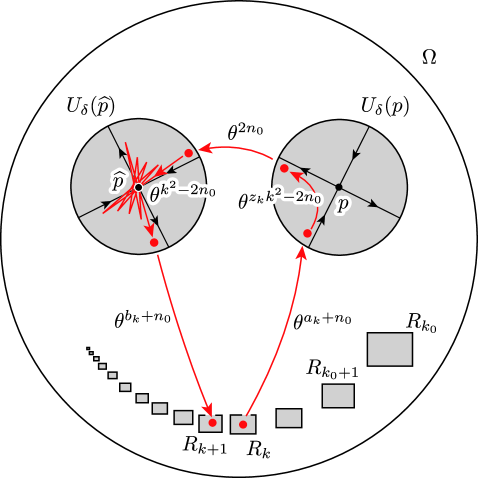
Figure 4. Travel from $R_{k}$ to $\mathrm{Int}R_{k+1}$ via $\theta^{m_{k}}$. The case where the eigenvalues of $D\theta(p)$ are positive and those of $D\theta(\hat{p})$ are negative.

For a given monotone increasing sequence $\{k(J^{\prime})\}_{J^{\prime}=1}^{\infty}$ of integers with $k(1)>k_{0}$, the sequence $\boldsymbol{z}=\{z_{k}\}_{k=k_{0}}^{\infty}$ is constructed to satisfy

$$z_{k}=z_{0}\quad\text{if $J^{\prime}$ is odd\quad and}\quad z_{k}=z_{0}+1\quad\text{if $J^{\prime}$ is even}$$

for any $k(J^{\prime}-1)<k\leq k(J^{\prime})$.

Now we will show that the sequence $\{k(J^{\prime})\}_{J^{\prime}=1}^{\infty}$ can be taken so that the following inequality holds: For any $\nu\geq 0$ and $\delta>0$, there is an integer $J^{\prime}_{0}\geq 1$ such that if $J^{\prime}\geq J^{\prime}_{0}$, then

(2.8) $$\frac{N_{\nu}(\omega,U_{\delta}(p);\hat{m}_{k(J^{\prime})})}{\hat{m}_{k(J^{\prime})}}\geq\frac{z_{*}}{z_{*}+1}-2^{-J^{\prime}},$$

where $z_{*}=z_{0}$ if $J^{\prime}$ is odd and $z_{*}=z_{0}+1$ if $J^{\prime}$ is even. It follows from (C2) that

$$\frac{N_{\nu}(\omega,U_{\delta}(p);\hat{m}_{k(J^{\prime})})}{\hat{m}_{k(J^{\prime})}} \geq\frac{\sum_{k=k(J^{\prime}-1)+1}^{k(J^{\prime})}(z_{k}k^{2}-2n_{0}-\nu)}{\hat{m}_{k(J^{\prime})}}$$

$$=\frac{\sum_{k=k(J^{\prime}-1)+1}^{k(J^{\prime})}(z_{k}k^{2}-2n_{0}-\nu)}{\sum_{k=k(J^{\prime}-1)+1}^{k(J^{\prime})}((z_{k}+1)k^{2}+a_{k}+b_{k})}\left(1-\frac{\hat{m}_{k(J^{\prime}-1)}}{\hat{m}_{k(J^{\prime})}}\right),$$

for each $\nu\geq 0$, $\delta>0$ and sufficiently large $J^{\prime}\geq 1$. On the other hand, it is easy to check that

$$\frac{\sum_{k=k(J^{\prime}-1)+1}^{k(J^{\prime})}(z_{k}k^{2}-2n_{0}-\nu)}{\sum_{k=k(J^{\prime}-1)+1}^{k(J^{\prime})}((z_{k}+1)k^{2}+a_{k}+b_{k})}=\frac{z_{*}-Z_{1}}{z_{*}+1+Z_{2}},$$

where $Z_{1}=\sum_{k=k(J^{\prime}-1)+1}^{k(J^{\prime})}(2n_{0}+\nu)/\sum_{k=k(J^{\prime}-1)+1}^{k(J^{\prime})}k^{2}$ and $Z_{2}=\sum_{k=k(J^{\prime}-1)+1}^{k(J^{\prime})}(a_{k}+b_{k})/\sum_{k=k(J^{\prime}-1)+1}^{k(J^{\prime})}k^{2}$. By taking $k(J^{\prime})$ sufficiently larger than $k(J^{\prime}-1)$, one can suppose that all of $\hat{m}_{k(J^{\prime}-1)}/\hat{m}_{k(J^{\prime})}$, $Z_{1}$ and $Z_{2}$ are arbitrarily close to zero. Thus there exists a sequence $\{k(J^{\prime})\}_{J^{\prime}=1}^{\infty}$ satisfying (2.8).

In a similar manner, we also can get that

(2.9) $$\frac{N_{\nu}(\omega,U_{\delta}(\hat{p});\hat{m}_{k(J^{\prime})})}{\hat{m}_{k(J^{\prime})}}\geq\frac{\sum_{k=k(J^{\prime}-1)+1}^{k(J^{\prime})}\left({k}^{2}-2n_{0}-n_{1}\right)}{\hat{m}_{k(J^{\prime})}}\geq\frac{1}{z_{*}+1}-2^{-J^{\prime}}.$$

Since $\frac{z_{*}}{z_{*}+1}+\frac{1}{z_{*}+1}=1$, (2.8) and (2.9) completes the proof of Theorem C with $\lambda_{1}=\frac{1}{z_{0}+1}$, $\lambda_{2}=\frac{1}{z_{0}+2}$ and $n_{1}(J)=\hat{m}_{k(2J-1)}$, $n_{2}(J)=\hat{m}_{k(2J)}$.

Appendix A The definition of absolute continuity

In this appendix, we compare Theorem A with Araújo’s result in [1] from the viewpoint of absolute continuity of a parametrised family of $\mathscr{C}^{r}$ diffeomorphisms. A parametrised family $\tilde{f}$ of $\mathscr{C}^{r}$ diffeomorphisms on a closed smooth Riemannian manifold $M$ is a differential mapping from $B\times M$ to $M$ such that $\tilde{f}_{t}\equiv\tilde{f}(t,\cdot):M\to M$ is a $\mathscr{C}^{r}$ diffeomorphism for all $t\in B$, where $B$ is the unit ball of a Euclidean space. Let $(B^{\mathbb{N}_{0}},\mathcal{B}(B)^{\mathbb{N}_{0}},\mathrm{Leb}_{B}^{\mathbb{N}_{0}})$ be the product space of a probability space $(B,\mathcal{B}(B),\mathrm{Leb}_{B})$, where $\mathcal{B}(B)$ is the Borel $\sigma$-field of $B$ and $\mathrm{Leb}_{B}$ is the normalised Lebesgue measure on $B$. For each $n\geq 1$, $\bar{t}=(t_{0},t_{1},\ldots)\in B^{\mathbb{N}_{0}}$ and $x\in M$, we define $\tilde{f}^{(n)}_{\bar{t}}(x)$ by

$$\tilde{f}^{(n)}_{\bar{t}}(x)=\tilde{f}_{t_{n-1}}\circ\tilde{f}_{t_{n-2}}\circ\cdots\circ\tilde{f}_{t_{0}}(x),$$

and let $\tilde{f}^{(n)}_{\bar{t}}=\mathrm{id}_{M}$ for all $\bar{t}\in B^{\mathbb{N}_{0}}$. Let $\mathrm{Leb}_{M}$ be the normalised Lebesgue measure on $M$. The following condition is from [1, Theorem 1].

Definition 7.

Let $\tilde{f}:B\times M\to M$ be a parametrised family of $\mathscr{C}^{r}$ diffeomorphisms. We say that $\tilde{f}$ is absolutely continuous if there exists an integer $N\geq 1$ and a real number $\xi>0$ such that for all $n\geq N$ and $x\in M$,

(A.1) $$\text{$\{\tilde{f}_{\bar{t}}^{(n)}(x)\mid\bar{t}\in B^{\mathbb{N}_{0}}\}$ contains the ball with radius $\xi$ centred at $f_{0}^{n}(x)$},$$

(A.2) $$\left(\tilde{f}_{(\cdot)}^{(n)}(x)\right)_{*}\mathrm{Leb}_{B}^{\mathbb{N}_{0}} \mathrm{Leb}_{M}$$ is absolutely continuous with respect to ,

where $0$ is the centre of $B$ and $(\tilde{f}_{(\cdot)}^{(n)}(x))_{*}$ is the pushforward of measures by $\tilde{f}_{(\cdot)}^{(n)}(x):B^{\mathbb{N}_{0}}\to M$ (the measurability of $\tilde{f}_{(\cdot)}^{(n)}(x)$ is ensured by [1, Property 2.1]).

Note that the deterministic case (i.e., the case when $\tilde{f}_{t}=\tilde{f}_{0}$ for all $t\in B$) is excluded by assuming that $\tilde{f}$ is absolutely continuous.

Let $\theta:B^{\mathbb{N}_{0}}\to B^{\mathbb{N}_{0}}$ be the one-sided shift, i.e., a measurable mapping given by $\theta(\bar{t})=(t_{1},t_{2},\ldots)$ for each $\bar{t}=(t_{0},t_{1},\ldots)$. Given a parametrised family $\tilde{f}:B\times M\to M$ of $\mathscr{C}^{r}$ diffeomorphisms, we define a mapping $F:\mathbb{N}_{0}\times B^{\mathbb{N}_{0}}\times M\to M$ by

$$F(n,\bar{t},x)=\tilde{f}^{(n)}_{\bar{t}}(x),\quad(n,\bar{t},x)\in\mathbb{N}_{0}\times B^{\mathbb{N}_{0}}\times M.$$

Then, it is straightforward to see that $F$ is an NDS over $\theta$ on base space $(\Omega,\mathcal{F},\mathbb{P})=(B^{\mathbb{N}_{0}},\mathcal{B}(B)^{\mathbb{N}_{0}},\mathrm{Leb}_{B}^{\mathbb{N}_{0}})$. Notice that the $B$-valued random process $\{\omega=(t_{0},t_{1},\ldots)\mapsto t_{n}\}_{n\geq 0}$ on $(\Omega,\mathcal{F},\mathbb{P})$ is independent and identically distributed, so that we call $F$ an i.i.d. nonautonomous dynamical system of $\tilde{f}$. We also note that $\theta$ is measure-preserving, i.e., an i.i.d. NDS is a random dynamical system.

The following theorem is an immediate consequence of [1, Theorem 1].

Theorem 8 (Araújo).

Let $F$ be an i.i.d. nonautonomous dynamical system of a parametrised family $\tilde{f}$ of $\mathscr{C}^{r}$ diffeomorphisms. Suppose that $\tilde{f}$ is absolutely continuous. Then for $\mathbb{P}$-almost every $\omega\in\Omega$, the set of points with historic behaviour at $\omega$ is a zero Lebesgue measure set.

We show that our parametrised perturbation is also absolutely continuous. In order to avoid notational confusion, we introduce another form for the mapping given in (1.4). Let $M$ be the circle $\mathbb{S}^{1}=\mathbb{R}/\mathbb{Z}$ and $B$ the unit disk of a Euclidean space. We define a parametrised perturbation $\tilde{f}:B\times M\to M$ of $\mathscr{C}^{r}$ diffeomorphisms by

(A.3) $$\tilde{f}(t,x)=f_{0}(x)+\epsilon\kappa(t)\mod 1,\quad(t,x)\in B\times M,$$

where $f_{0}$ is the $\mathscr{C}^{r}$ mapping given in (1.3) and $\kappa:B\to[-1,1]$ is a surjective continuous function such that $\kappa_{*}\mathrm{Leb}_{B}$ is absolute continuous with respect to $\mathrm{Leb}_{M}$.

Proposition 9.

Let $\tilde{f}$ be a parametrised family of $\mathscr{C}^{r}$ diffeomorphisms given in (A.3). Then $\tilde{f}$ is absolutely continuous.

We note that, although the parametrised family $\tilde{f}$ is absolutely continuous, the driving system of our NDS in Theorem A is completely different from the driving system of i.i.d. NDS’s (i.e., the one-sided shift) in the sense of historic behaviour (as in Remark 2), which may cause the difference between our and Araújo’s results.

Proof of Proposition 9.

We first see that (A.1) holds, so fix $n\geq 1$ and $x\in\mathbb{S}^{1}$. Due to that $\tilde{f}^{(n)}_{\bar{t}}(x)=\tilde{f}_{t_{n-1}}(\tilde{f}_{\bar{t}}^{(n-1)}(x))$ for each $\bar{t}\in B^{\mathbb{N}_{0}}$, $\{\tilde{f}^{(n)}_{\bar{t}}(x)\mid\bar{t}\in B^{\mathbb{N}_{0}}\}$ contains $\{\tilde{f}_{t}(\tilde{f}^{n-1}_{0}(x))\mid t\in B\}$. Furthermore, by virtue of (A.3), $\{\tilde{f}_{t}(\tilde{f}^{n-1}_{0}(x))\mid t\in B\}$ coincides with the ball with radius $\epsilon$ centred at $\tilde{f}_{0}^{n-1}(x)$. Therefore (A.1) holds with $N=1$ and $\xi=\epsilon$.

Arguing by induction, we first see that (A.2) holds for $n=1$. For any $x\in\mathbb{S}^{1}$ and Borel set $A\subset\mathbb{S}^{1}$, if we let $\frac{A-f_{0}(x)}{\epsilon}=\{y\in\mathbb{R}\mid f_{0}(x)+\epsilon y\in A\}$, then

$$\left(\tilde{f}^{(1)}_{(\cdot)}(x)\right)_{*}\mathrm{Leb}_{B}^{\mathbb{N}_{0}}(A)=\mathrm{Leb}_{B}\left(\left\{t\in B\mid f_{0}(x)+\epsilon\kappa(t)\in\tilde{A}\right\}\right)$$

coincides with $\kappa_{*}\mathrm{Leb}_{B}(\frac{A-f_{0}(x)}{\epsilon})$. If $\mathrm{Leb}_{\mathbb{R}}(A)=0$, then obviously $\mathrm{Leb}_{\mathbb{R}}(\frac{A-f_{0}(x)}{\epsilon})=0$, so we get $\kappa_{*}\mathrm{Leb}_{B}(\frac{A-f_{0}(x)}{\epsilon})=0$ due to the absolute continuity of $\kappa_{*}\mathrm{Leb}_{B}$. That is, (A.2) holds with $n=1$.

Suppose that (A.2) holds for $n=k$. For any $x\in\mathbb{S}^{1}$ and Borel set $A\subset\mathbb{S}^{1}$, $(\tilde{f}^{(k+1)}_{(\cdot)}(x))_{*}\mathrm{Leb}_{B}^{\mathbb{N}_{0}}(A)$ coincides with

(A.4) $$\int\mathrm{Leb}_{B}^{\mathbb{N}_{0}}\left(\left\{\bar{t}\in B^{\mathbb{N}_{0}}\mid\tilde{f}^{(k)}_{\bar{t}}(x)\in\tilde{f}_{t}^{-1}(A)\right\}\right)d\mathrm{Leb}_{B}(t).$$

On the other hand, if $\mathrm{Leb}_{\mathbb{R}}(A)=0$, then $\mathrm{Leb}_{\mathbb{R}}(f_{t}^{-1}(A))=0$ for any $t\in B$ since $\mathrm{Leb}_{\mathbb{S}^{1}}(\tilde{f}_{t}^{-1}(A))\leq\sup_{x}|D\tilde{f}_{t}^{-1}(x)|\mathrm{Leb}_{\mathbb{S}^{1}}(A)$. Hence, by the inductive step, we get $\mathrm{Leb}_{B}^{\mathbb{N}_{0}}(\{\bar{t}\in B^{\mathbb{N}_{0}}\mid\tilde{f}^{(k)}_{\bar{t}}(x)\in\tilde{f}_{t}^{-1}(A)\})=0$ for each $t\in B$, and (A.2) with $n=k+1$ follows from (A.4). ∎

Appendix B Proof of Proposition 3

We shall first find an essentially bounded mapping $Y:\Omega\to I_{0}$, which is invariant under $f$, i.e., $f_{\omega}(Y(\omega))=Y(\theta\omega)$ $\mathbb{P}$-almost surely, under the identification of $I_{0}$ with $[\frac{1}{4},\frac{3}{4}]$ by $\pi_{M}$. Let $L^{\infty}(\Omega,I_{0})$ be the space of measurable mappings $b\in L^{\infty}(\Omega,\mathbb{R})$ whose essential supremum norm $\|b\|_{L^{\infty}}$ is in $I_{0}$. For each $b\in L^{\infty}(\Omega,I_{0})$, we define a mapping $\mathcal{G}(b):\Omega\to I_{0}$ by

$$\mathcal{G}(b)(\omega)=f_{\theta^{-1}\omega}\left(b(\theta^{-1}\omega)\right),\quad\omega\in\Omega.$$

Then, it is easy to see that $\mathcal{G}(b)$ is in $L^{\infty}(\Omega,I_{0})$: Note that $\mathcal{G}(b)$ is the composition of two measurable mappings $\omega\mapsto f_{\omega}\left(b(\omega)\right)=f_{0}\circ b(\omega)+\epsilon\kappa(\omega)$ and $\theta^{-1}$. (The transformation $\mathcal{G}:L^{\infty}(\Omega,I_{0})\to L^{\infty}(\Omega,I_{0})$ is called the graph transformation induced by $f$.) Furthermore, by virtue of (1.3) and (1.5), we have

$$\left\|\mathcal{G}(b_{1})-\mathcal{G}(b_{2})\right\|_{L^{\infty}} =\operatorname*{ess\,sup}_{\omega\in\Omega}\left|f_{\theta^{-1}\omega}\left(b_{1}(\theta^{-1}\omega)\right)-f_{\theta^{-1}\omega}\left(b_{2}(\theta^{-1}\omega)\right)\right|$$

$$=\frac{1}{2}\operatorname*{ess\,sup}_{\omega\in\Omega}\left|b_{1}(\theta^{-1}\omega)-b_{2}(\theta^{-1}\omega)\right|=\frac{1}{2}\|b_{1}-b_{2}\|_{L^{\infty}},$$

for all $b_{1},b_{2}\in L^{\infty}(\Omega,I_{0})$, i.e., $\mathcal{G}$ is a contraction mapping on the complete metric space $L^{\infty}(\Omega,I_{0})$. Therefore, there exists a unique fixed point $Y$ of $\mathcal{G}$. By construction, $Y:\Omega\to I_{0}$ is an $f$-invariant essentially bounded mapping.

Fix a continuous mapping $\varphi:M\to\mathbb{R}$. Since $M$ is compact, $\varphi$ is uniformly continuous. On the other hand, due to the invariance of $Y$ together with (1.3) and (1.4), we have

(B.1) $$\left|f^{(n)}_{\omega}(x)-Y(\theta^{n}\omega)\right| =\left|f^{(n)}_{\omega}(x)-f^{(n)}_{\omega}(Y(\omega))\right|$$

$$=\frac{1}{2^{n}}\left|x-Y(\omega)\right|\to 0$$

as $n$ goes to infinity for $\mathbb{P}$-almost every $\omega$ and all $x$ in $I_{0}$. Therefore, a straightforward calculation shows that

$$\left|\frac{1}{n}\sum_{j=0}^{n-1}\varphi(f^{(j)}_{\omega}(x))-\frac{1}{n}\sum_{j=0}^{n-1}\varphi(Y(\theta^{n}\omega))\right|\to 0$$

as $n$ goes to infinity for $\mathbb{P}$-almost every $\omega$ and all $x$ in $I_{0}$. Since $\varphi\circ Y$ is an integrable function, we get the conclusion from the fact that $\theta$ is non-historic.

References

- [1] V. Araújo, Attractors and time averages for random maps, Ann. lnst. H. Poincaré Anal. Non Linéaire 17 (2000), 307–369.
- [2] V. Araújo, H. Aytaç, Decay of correlations and laws of rare events for transitive random maps, Nonlinearity 30 no. 5 (2017), 1834.
- [3] V. Araujo, V. Pinheiro, Abundance of wild historic behavior, ergodic decomposition and generalized physical measures, arXiv preprint arXiv:1609.05356 (2016).
- [4] L. Arnold, Random dynamical systems, Springer, 1998.
- [5] V. Baladi, A. Kondah, B. Schmitt, Random correlations for small perturbations of expanding maps, Random Comput. Dynam. 4 no. 2/3 (1996), 179–204.
- [6] C. Bonatti, L. Díaz, M. Viana, Dynamics Beyond Uniform Hyperbolicity: A Global Geometric and Probabilistic Perspective, Encyclopaedia of Mathematical Science 102, Springer-Verlag, 2004.
- [7] C. González-Tokman, Multiplicative ergodic theorems for transfer operators: towards the identification and analysis of coherent structures in non-autonomous dynamical systems, (2016).
- [8] J. Jürgen, M. Kell, C. S. Rodrigues, Representation of Markov chains by random maps: existence and regularity conditions, Calc. Var. Partial Differential Equations 54 no. 3 (2015), 2637–2655.
- [9] P. E. Kloeden, M. Rasmussen, Nonautonomous dynamical systems (No. 176), American Mathematical Soc., 2011.
- [10] S. Kiriki, T. Soma, Takens’ last problem and existence of non-trivial wandering domains, Adv. Math. 306 (2017), 524–588.
- [11] I. S. Labouriau, A. A. P. Rodrigues, On Takens’ Last Problem: tangencies and time averages near heteroclinic networks, Nonlinearity 30 no. 5 (2016), 1876.
- [12] M. C. Mackey, M. Tyran-Kamińska, Deterministic Brownian motion: The effects of perturbing a dynamical system by a chaotic semi-dynamical system, Physics reports 422 no. 5 (2006), 167–222.
- [13] Y. Nakano, Historic Behaviour for Random Expanding Maps on the Circle, Tokyo Journal of Mathematics 40 no. 1 (2017), 165–184.
- [14] Y. Nakano, M. Tsujii, J. Wittsten, The partial captivity condition for U(1) extensions of expanding maps on the circle, Nonlinearity 29 (2016), 1917.
- [15] S. Newhouse, The abundance of wild hyperbolic sets and non-smooth stable sets for diffeomorphisms, Publ. Math. I.H.É.S. 50 (1979), 101–151.
- [16] D. Ruelle, Historical behaviour in smooth dynamical systems, Global Analysis of Dynamical Systems, eds. H. W. Broer et al, Institute of Physics Publishing, 2001.
- [17] F. Takens, Heteroclinic attractors: time averages and moduli of topological conjugacy, Bol. Soc. Bras. Mat. 25 (1994), 107–120.
- [18] F. Takens, Orbits with historic behaviour, or non-existence of averages, Nonlinearity 21 no. 1 (2008), T33–T36.