A Structured Self-attentive Sentence Embedding
A Structured Self-attentive
Sentence Embedding
Abstract
This paper proposes a new model for extracting an interpretable sentence embedding by introducing self-attention. Instead of using a vector, we use a 2-D matrix to represent the embedding, with each row of the matrix attending on a different part of the sentence. We also propose a self-attention mechanism and a special regularization term for the model. As a side effect, the embedding comes with an easy way of visualizing what specific parts of the sentence are encoded into the embedding. We evaluate our model on 3 different tasks: author profiling, sentiment classification and textual entailment. Results show that our model yields a significant performance gain compared to other sentence embedding methods in all of the 3 tasks.
1 Introduction
Much progress has been made in learning semantically meaningful distributed representations of individual words, also known as word embeddings (Bengio et al., 2001; Mikolov et al., 2013). On the other hand, much remains to be done to obtain satisfying representations of phrases and sentences. Those methods generally fall into two categories. The first consists of universal sentence embeddings usually trained by unsupervised learning (Hill et al., 2016). This includes SkipThought vectors (Kiros et al., 2015), ParagraphVector (Le & Mikolov, 2014), recursive auto-encoders (Socher et al., 2011; 2013), Sequential Denoising Autoencoders (SDAE), FastSent (Hill et al., 2016), etc.
The other category consists of models trained specifically for a certain task. They are usually combined with downstream applications and trained by supervised learning. One generally finds that specifically trained sentence embeddings perform better than generic ones, although generic ones can be used in a semi-supervised setting, exploiting large unlabeled corpora. Several models have been proposed along this line, by using recurrent networks (Hochreiter & Schmidhuber, 1997; Chung et al., 2014), recursive networks (Socher et al., 2013) and convolutional networks (Kalchbrenner et al., 2014; dos Santos & Gatti, 2014; Kim, 2014) as an intermediate step in creating sentence representations to solve a wide variety of tasks including classification and ranking (Yin & Schütze, 2015; Palangi et al., 2016; Tan et al., 2016; Feng et al., 2015). A common approach in previous methods consists in creating a simple vector representation by using the final hidden state of the RNN or the max (or average) pooling from either RNNs hidden states or convolved n-grams. Additional works have also been done in exploiting linguistic structures such as parse and dependence trees to improve sentence representations (Ma et al., 2015; Mou et al., 2015b; Tai et al., 2015).
For some tasks people propose to use attention mechanism on top of the CNN or LSTM model to introduce extra source of information to guide the extraction of sentence embedding (dos Santos et al., 2016). However, for some other tasks like sentiment classification, this is not directly applicable since there is no such extra information: the model is only given one single sentence as input. In those cases, the most common way is to add a max pooling or averaging step across all time steps (Lee & Dernoncourt, 2016), or just pick up the hidden representation at the last time step as the encoded embedding (Margarit & Subramaniam, 2016).
A common approach in many of the aforementioned methods consists of creating a simple vector representation by using the final hidden state of the RNN or the max (or average) pooling from either RNNs hidden states or convolved n-grams. We hypothesize that carrying the semantics along all time steps of a recurrent model is relatively hard and not necessary. We propose a self-attention mechanism for these sequential models to replace the max pooling or averaging step. Different from previous approaches, the proposed self-attention mechanism allows extracting different aspects of the sentence into multiple vector representations. It is performed on top of an LSTM in our sentence embedding model. This enables attention to be used in those cases when there are no extra inputs. In addition, due to its direct access to hidden representations from previous time steps, it relieves some long-term memorization burden from LSTM. As a side effect coming together with our proposed self-attentive sentence embedding, interpreting the extracted embedding becomes very easy and explicit.
Section 2 details on our proposed self-attentive sentence embedding model, as well as a regularization term we proposed for this model, which is described in Section 2.2. We also provide a visualization method for this sentence embedding in section 2.3. We then evaluate our model in author profiling, sentiment classification and textual entailment tasks in Section 4.
2 Approach
2.1 Model
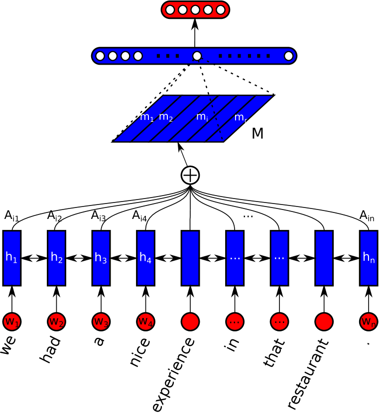
The proposed sentence embedding model consists of two parts. The first part is a bidirectional LSTM, and the second part is the self-attention mechanism, which provides a set of summation weight vectors for the LSTM hidden states. These set of summation weight vectors are dotted with the LSTM hidden states, and the resulting weighted LSTM hidden states are considered as an embedding for the sentence. It can be combined with, for example, a multilayer perceptron to be applied on a downstream application. Figure 1 shows an example when the proposed sentence embedding model is applied to sentiment analysis, combined with a fully connected layer and a softmax layer. Besides using a fully connected layer, we also proposes an approach that prunes weight connections by utilizing the 2-D structure of matrix sentence embedding, which is detailed in Appendix A. For this section, we will use Figure 1 to describe our model.
Suppose we have a sentence, which has tokens, represented in a sequence of word embeddings.
| (1) |
Here is a vector standing for a dimentional word embedding for the -th word in the sentence. is thus a sequence represented as a 2-D matrix, which concatenates all the word embeddings together. should have the shape -by-.
Now each entry in the sequence are independent with each other. To gain some dependency between adjacent words within a single sentence, we use a bidirectional LSTM to process the sentence:
| (2) |
| (3) |
And we concatenate each with to obtain a hidden state . Let the hidden unit number for each unidirectional LSTM be . For simplicity, we note all the s as , who have the size -by-.
| (4) |
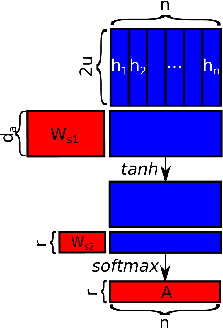
Our aim is to encode a variable length sentence into a fixed size embedding. We achieve that by choosing a linear combination of the LSTM hidden vectors in . Computing the linear combination requires the self-attention mechanism. The attention mechanism takes the whole LSTM hidden states as input, and outputs a vector of weights :
| (5) |
Here is a weight matrix with a shape of -by-. and is a vector of parameters with size , where is a hyperparameter we can set arbitrarily. Since is sized -by-, the annotation vector will have a size . the ensures all the computed weights sum up to 1. Then we sum up the LSTM hidden states according to the weight provided by to get a vector representation of the input sentence.
This vector representation usually focuses on a specific component of the sentence, like a special set of related words or phrases. So it is expected to reflect an aspect, or component of the semantics in a sentence. However, there can be multiple components in a sentence that together forms the overall semantics of the whole sentence, especially for long sentences. (For example, two clauses linked together by an ”and.”) Thus, to represent the overall semantics of the sentence, we need multiple ’s that focus on different parts of the sentence. Thus we need to perform multiple hops of attention. Say we want different parts to be extracted from the sentence, with regard to this, we extend the into a -by- matrix, note it as , and the resulting annotation vector becomes annotation matrix . Formally,
| (6) |
Here the is performed along the second dimension of its input. We can deem Equation 6 as a 2-layer MLP without bias, whose hidden unit numbers is , and parameters are .
The embedding vector then becomes an -by- embedding matrix . We compute the weighted sums by multiplying the annotation matrix and LSTM hidden states , the resulting matrix is the sentence embedding:
| (7) |
2.2 Penalization term
The embedding matrix can suffer from redundancy problems if the attention mechanism always provides similar summation weights for all the hops. Thus we need a penalization term to encourage the diversity of summation weight vectors across different hops of attention.
The best way to evaluate the diversity is definitely the Kullback – Leibler divergence between any 2 of the summation weight vectors. However, we found that not very stable in our case. We conjecture it is because we are maximizing a set of KL divergence (instead of minimizing only one, which is the usual case), we are optimizing the annotation matrix A to have a lot of sufficiently small or even zero values at different softmax output units, and these vast amount of zeros is making the training unstable. There is another feature that KL doesn’t provide but we want, which is, we want each individual row to focus on a single aspect of semantics, so we want the probability mass in the annotation softmax output to be more focused. but with KL penalty we can’t encourage that.
We hereby introduce a new penalization term which overcomes the aforementioned shortcomings. Compared to the KL divergence penalization, this term consumes only one third of the computation. We use the dot product of and its transpose, subtracted by an identity matrix, as a measure of redundancy.
| (8) |
Here stands for the Frobenius norm of a matrix. Similar to adding an L2 regularization term, this penalization term will be multiplied by a coefficient, and we minimize it together with the original loss, which is dependent on the downstream application.
Let’s consider two different summation vectors and in . Because of the softmax, all entries within any summation vector in should sum up to 1. Thus they can be deemed as probability masses in a discrete probability distribution. For any non-diagonal elements in the matrix, it corresponds to a summation over elementwise product of two distributions:
| (9) |
where and are the -th element in the and vectors, respectively. In the most extreme case, where there is no overlap between the two probability distributions and , the correspond will be 0. Otherwise, it will have a positive value. On the other extreme end, if the two distributions are identical and all concentrates on one single word, it will have a maximum value of 1. We subtract an identity matrix from so that forces the elements on the diagonal of to approximate 1, which encourages each summation vector to focus on as few number of words as possible, forcing each vector to be focused on a single aspect, and all other elements to 0, which punishes redundancy between different summation vectors.
2.3 Visualization
The interpretation of the sentence embedding is quite straight forward because of the existence of annotation matrix . For each row in the sentence embedding matrix , we have its corresponding annotation vector . Each element in this vector corresponds to how much contribution the LSTM hidden state of a token on that position contributes to. We can thus draw a heat map for each row of the embedding matrix This way of visualization gives hints on what is encoded in each part of the embedding, adding an extra layer of interpretation. (See Figure 3(a) and 3(b)).
The second way of visualization can be achieved by summing up over all the annotation vectors, and then normalizing the resulting weight vector to sum up to 1. Since it sums up all aspects of semantics of a sentence, it yields a general view of what the embedding mostly focuses on. We can figure out which words the embedding takes into account a lot, and which ones are skipped by the embedding. See Figure 3(c) and 3(d).
3 Related work
Various supervised and unsupervised sentence embedding models have been mentioned in Section 1. Different from those models, our proposed method uses a new self-attention mechanism that allows it to extract different aspects of the sentence into multiple vector-representations. The matrix structure together with the penalization term gives our model a greater capacity to disentangle the latent information from the input sentence. We also do not use linguistic structures to guide our sentence representation model. Additionally, using our method we can easily create visualizations that can help in the interpretation of the learned representations.
Some recent work have also proposed supervised methods that use intra/self-sentence attention. Ling et al. (2015) proposed an attention based model for word embedding, which calculates an attention weight for each word at each possible position in the context window. However this method cannot be extended to sentence level embeddings since one cannot exhaustively enumerate all possible sentences. Liu et al. (2016a) proposes a sentence level attention which has a similar motivation but done differently. They utilize the mean pooling over LSTM states as the attention source, and use that to re-weight the pooled vector representation of the sentence.
Apart from the previous 2 variants, we want to note that Li et al. (2016) proposed a same self attention mechanism for question encoding in their factoid QA model, which is concurrent to our work. The difference lies in that their encoding is still presented as a vector, but our attention produces a matrix representation instead, with a specially designed penalty term. We applied the model for sentiment anaysis and entailment, and their model is for factoid QA.
The LSTMN model (Cheng et al., 2016) also proposed a very successful intra-sentence level attention mechanism, which is later used by Parikh et al. (2016). We see our attention and theirs as having different granularities. LSTMN produces an attention vector for each of its hidden states during the recurrent iteration, which is sort of an ”online updating” attention. It’s more fine-grained, targeting at discovering lexical correlations between a certain word and its previous words. On the contrary, our attention mechanism is only performed once, focuses directly on the semantics that makes sense for discriminating the targets. It is less focused on relations between words, but more on the semantics of the whole sentence that each word contributes to. Computationally, our method also scales up with the sentence length better, since it doesn’t require the LSTM to compute an annotation vector over all of its previous words each time when the LSTMN computes its next step.
4 Experimental results
We first evaluate our sentence embedding model by applying it to 3 different datasets: the Age dataset, the Yelp dataset, and the Stanford Natural Language Inference (SNLI) Corpus. These 3 datasets fall into 3 different tasks, corresponding to author profiling, sentiment analysis, and textual entailment, respectively. Then we also perform a set of exploratory experiments to validate properties of various aspects for our sentence embedding model.
4.1 Author profiling
The Author Profiling dataset111http://pan.webis.de/clef16/pan16-web/author-profiling.html consists of Twitter tweets in English, Spanish, and Dutch. For some of the tweets, it also provides an age and gender of the user when writing the tweet. The age range are split into 5 classes: 18-24, 25-34, 35-49, 50-64, 65+. We use English tweets as input, and use those tweets to predict the age range of the user. Since we are predicting the age of users, we refer to it as Age dataset in the rest of our paper. We randomly selected 68485 tweets as training set, 4000 for development set, and 4000 for test set. Performances are also chosen to be classification accuracy.
| Models | Yelp | Age |
|---|---|---|
| BiLSTM + Max Pooling + MLP | 61.99% | 77.40% |
| CNN + Max Pooling + MLP | 62.05% | 78.15% |
| Our Model | 64.21% | 80.45% |
We compare our model with two baseline models: biLSTM and CNN. For the two baseline models. The biLSTM model uses a bidirectional LSTM with 300 dimensions in each direction, and use max pooling across all LSTM hidden states to get the sentence embedding vector, then use a 2-layer ReLU output MLP with 3000 hidden states to output the classification result. The CNN model uses the same scheme, but substituting biLSTM with 1 layer of 1-D convolutional network. During training we use 0.5 dropout on the MLP and 0.0001 L2 regularization. We use stochastic gradient descent as the optimizer, with a learning rate of 0.06, batch size 16. For biLSTM, we also clip the norm of gradients to be between -0.5 and 0.5. We searched hyperparameters in a wide range and find the aforementioned set of hyperparameters yields the highest accuracy.
For our model, we use the same settings as what we did in biLSTM. We also use a 2-layer ReLU output MLP, but with 2000 hidden units. In addition, our self-attention MLP has a hidden layer with 350 units (the in Section 2), we choose the matrix embedding to have 30 rows (the ), and a coefficient of 1 for the penalization term.
We train all the three models until convergence and select the corresponding test set performance according to the best development set performance. Our results show that the model outperforms both of the biLSTM and CNN baselines by a significant margin.
4.2 Sentiment analysis


We choose the Yelp dataset222https://www.yelp.com/dataset_challenge for sentiment analysis task. It consists of 2.7M yelp reviews, we take the review as input and predict the number of stars the user who wrote that review assigned to the corresponding business store. We randomly select 500K review-star pairs as training set, and 2000 for development set, 2000 for test set. We tokenize the review texts by Stanford tokenizer. We use 100 dimensional word2vec as initialization for word embeddings, and tune the embedding during training across all of our experiments. The target number of stars is an integer number in the range of , inclusive. We are treating the task as a classification task, i.e., classify a review text into one of the 5 classes. We use classification accuracy as a measurement.
For the two baseline models, we use the same setting as what we used for Author Profiling dataset, except that we are using a batch size of 32 instead. For our model, we are also using the same setting, except that we choose the hidden unit numbers in the output MLP to be 3000 instead. We also observe a significant performance gain comparining to the two baselines. (Table 1)
As an interpretation of the learned sentence embedding, we use the second way of visualization described in Section 2.3 to plot heat maps for some of the reviews in the dataset. We randomly select 5 examples of negative (1 star) and positive (5 stars) reviews from the test set, when the model has a high confidence () in predicting the label. As shown in Figure 2, we find that the model majorly learns to capture some key factors in the review that indicate strongly on the sentiment behind the sentence. For most of the short reviews, the model manages to capture all the key factors that contribute to an extreme score, but for longer reviews, the model is still not able to capture all related factors. For example, in the 3rd review in Figure 2(b)), it seems that a lot of focus is spent on one single factor, i.e., the ”so much fun”, and the model puts a little amount of attention on other key points like ”highly recommend”, ”amazing food”, etc.
| Model | Test Accuracy |
|---|---|
| 300D LSTM encoders (Bowman et al., 2016) | 80.6% |
| 600D (300+300) BiLSTM encoders (Liu et al., 2016b) | 83.3% |
| 300D Tree-based CNN encoders (Mou et al., 2015a) | 82.1% |
| 300D SPINN-PI encoders (Bowman et al., 2016) | 83.2% |
| 300D NTI-SLSTM-LSTM encoders (Munkhdalai & Yu, 2016a) | 83.4% |
| 1024D GRU encoders with SkipThoughts pre-training (Vendrov et al., 2015) | 81.4% |
| 300D NSE encoders (Munkhdalai & Yu, 2016b) | 84.6% |
| Our method | 84.4% |
4.3 Textual entailment
We use the biggest dataset in textual entailment, the SNLI corpus (Bowman et al., 2015) for our evaluation on this task. SNLI is a collection of 570k human-written English sentence pairs manually labeled for balanced classification with the labels entailment, contradiction, and neutral. The model will be given a pair of sentences, called hypothesis and premise respectively, and asked to tell if the semantics in the two sentences are contradicting with each other or not. It is also a classification task, so we measure the performance by accuracy.
We process the hypothesis and premise independently, and then extract the relation between the two sentence embeddings by using multiplicative interactions proposed in Memisevic (2013) (see Appendix B for details), and use a 2-layer ReLU output MLP with 4000 hidden units to map the hidden representation into classification results. Parameters of biLSTM and attention MLP are shared across hypothesis and premise. The biLSTM is 300 dimension in each direction, the attention MLP has 150 hidden units instead, and both sentence embeddings for hypothesis and premise have 30 rows (the ). The penalization term coefficient is set to 0.3. We use 300 dimensional GloVe (Pennington et al., 2014) word embedding to initialize word embeddings. We use AdaGrad as the optimizer, with a learning rate of 0.01. We don’t use any extra regularization methods, like dropout or L2 normalization. Training converges after 4 epochs, which is relatively fast.
This task is a bit different from previous two tasks, in that it has 2 sentences as input. There are a bunch of ways to add inter-sentence level attention, and those attentions bring a lot of benefits. To make the comparison focused and fair, we only compare methods that fall into the sentence encoding-based models. i.e., there is no information exchanged between the hypothesis and premise before they are encoded into some distributed encoding.
We find that compared to other published approaches, our method shows a significant gain () to them, except for the 300D NSE encoders, which is the state-of-the-art in this category. However, the different is relatively small compared to the differences between other methods.
4.4 Exploratory experiments
In this subsection we are going to do a set of exploratory experiments to study the relative effect of each component in our model.
4.4.1 Effect of penalization term
Since the purpose of introducing the penalization term is majorly to discourage the redundancy in the embedding, we first directly visualize the heat maps of each row when the model is presented with a sentence. We compare two identical models with the same size as detailed in Section 4.1 trained separately on Age dataset, one with this penalization term (where the penalization coefficient is set to 1.0) and the other with no penalty. We randomly select one tweet from the test set and compare the two models by plotting a heat map for each hop of attention on that single tweet. Since there are 30 hops of attention for each model, which makes plotting all of them quite redundant, we only plot 6 of them. These 6 hops already reflect the situation in all of the 30 hops.
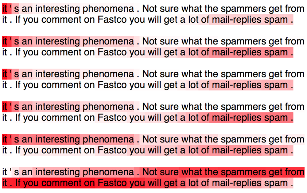
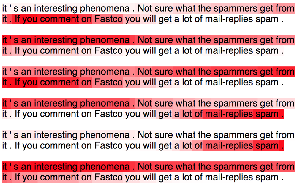


From the figure we can tell that the model trained without the penalization term have lots of redundancies between different hops of attention (Figure 3(a)), resulting in putting lot of focus on the word ”it” (Figure 3(c)), which is not so relevant to the age of the author. However in the right column, the model shows more variations between different hops, and as a result, the overall embedding focuses on ”mail-replies spam” instead. (Figure 3(d))
For the Yelp dataset, we also observe a similar phenomenon. To make the experiments more explorative, we choose to plot heat maps of overall attention heat maps for more samples, instead of plotting detailed heat maps for a single sample again. Figure 4 shows overall focus of the sentence embedding on three different reviews. We observe that with the penalization term, the model tends to be more focused on important parts of the review. We think it is because that we are encouraging it to be focused, in the diagonals of matrix (Equation 8).
To validate if these differences result in performance difference, we evaluate four models trained on Yelp and Age datasets, both with and without the penalization term. Results are shown in Table 3. Consistent with what expected, models trained with the penalization term outperforms their counterpart trained without.
| Penalization coefficient | Yelp | Age |
|---|---|---|
| 1.0 | 64.21% | 80.45% |
| 0.0 | 61.74% | 79.27% |
In SNLI dataset, although we observe that introducing the penalization term still contributes to encouraging the diversity of different rows in the matrix sentence embedding, and forcing the network to be more focused on the sentences, the quantitative effect of this penalization term is not so obvious on SNLI dataset. Both models yield similar test set accuracies.
4.4.2 Effect of multiple vectors
Having multiple rows in the sentence embedding is expected to provide more abundant information about the encoded content. It makes sence to evaluate how significant the improvement can be brought by . Taking the models we used for Age and SNLI dataset as an example, we vary from to for each task, and train the resulting models independently (Figure 5). Note that when , the sentence embedding reduces to a normal vector form.
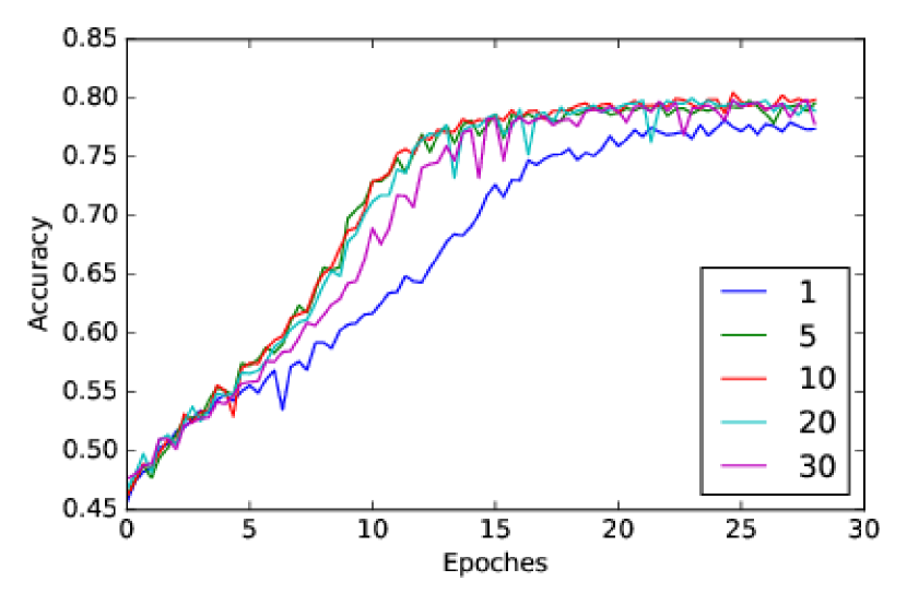
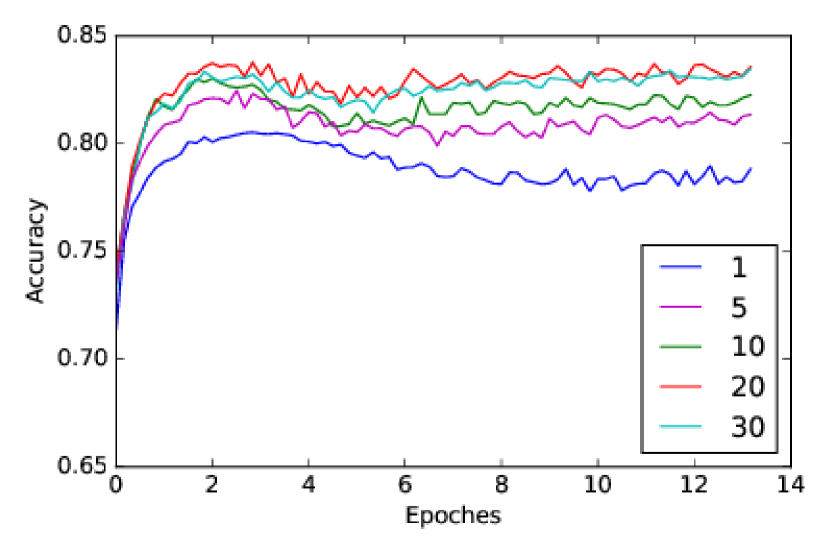
From this figure we can find that, without having multiple rows, the model performs on-par with its competitiors which use other forms of vector sentence embeddings. But there is significant difference between having only one vector for the sentence embedding and multiple vectors. The models are also quite invariant with respect to , since in the two figures a wide range of values between to are all generating comparable curves.
5 Conclusion and discussion
In this paper, we introduced a fixed size, matrix sentence embedding with a self-attention mechanism. Because of this attention mechanism, there is a way to interpret the sentence embedding in depth in our model. Experimental results over 3 different tasks show that the model outperforms other sentence embedding models by a significant margin.
Introducing attention mechanism allows the final sentence embedding to directly access previous LSTM hidden states via the attention summation. Thus the LSTM doesn’t need to carry every piece of information towards its last hidden state. Instead, each LSTM hidden state is only expected to provide shorter term context information around each word, while the higher level semantics, which requires longer term dependency, can be picked up directly by the attention mechanism. This setting reliefs the burden of LSTM to carry on long term dependencies. Our experiments also support that, as we observed that our model has a bigger advantage when the contents are longer. Further more, the notion of summing up elements in the attention mechanism is very primitive, it can be something more complex than that, which will allow more operations on the hidden states of LSTM.
The model is able to encode any sequence with variable length into a fixed size representation, without suffering from long-term dependency problems. This brings a lot of scalability to the model: without any modification, it can be applied directly to longer contents like paragraphs, articles, etc. Though this is beyond the focus of this paper, it remains an interesting direction to explore as a future work.
As a downside of our proposed model, the current training method heavily relies on downstream applications, thus we are not able to train it in an unsupervised way. The major obstacle towards enabling unsupervised learning in this model is that during decoding, we don’t know as prior how the different rows in the embedding should be divided and reorganized. Exploring all those possible divisions by using a neural network could easily end up with overfitting. Although we can still do unsupervised learning on the proposed model by using a sequential decoder on top of the sentence embedding, it merits more to find some other structures as a decoder.
Acknowledgments
The authors would like to acknowledge the developers of Theano (Theano Development Team, 2016) and Lasagne. The first author would also like to thank IBM Watson for providing resources, fundings and valuable discussions to make this project possible, and Caglar Gulcehre for helpful discussions.
References
- Bengio et al. (2001) Yoshua Bengio, Réjean Ducharme, and Pascal Vincent. A neural probabilistic language model. In Advances in Neural Information Processing Systems, pp. 932–938, 2001.
- Bowman et al. (2015) Samuel R Bowman, Gabor Angeli, Christopher Potts, and Christopher D Manning. A large annotated corpus for learning natural language inference. arXiv preprint arXiv:1508.05326, 2015.
- Bowman et al. (2016) Samuel R Bowman, Jon Gauthier, Abhinav Rastogi, Raghav Gupta, Christopher D Manning, and Christopher Potts. A fast unified model for parsing and sentence understanding. arXiv preprint arXiv:1603.06021, 2016.
- Cheng et al. (2016) Jianpeng Cheng, Li Dong, and Mirella Lapata. Long short-term memory-networks for machine reading. In Conference on Empirical Methods in Natural Language Processing (EMNLP). Association for Computational Linguistics, 2016.
- Chung et al. (2014) Junyoung Chung, Caglar Gulcehre, KyungHyun Cho, and Yoshua Bengio. Empirical evaluation of gated recurrent neural networks on sequence modeling. arXiv preprint arXiv:1412.3555, 2014.
- dos Santos & Gatti (2014) Cicero dos Santos and Maira Gatti. Deep convolutional neural networks for sentiment analysis of short texts. In Proceedings of COLING 2014, the 25th International Conference on Computational Linguistics: Technical Papers, pp. 69–78, 2014.
- dos Santos et al. (2016) Cicero dos Santos, Ming Tan, Bing Xiang, and Bowen Zhou. Attentive pooling networks. arXiv preprint arXiv:1602.03609, 2016.
- Feng et al. (2015) Minwei Feng, Bing Xiang, Michael R. Glass, Lidan Wang, and Bowen Zhou. Applying deep learning to answer selection: a study and an open task. In 2015 IEEE Workshop on Automatic Speech Recognition and Understanding, ASRU 2015, Scottsdale, AZ, USA, December 13-17, 2015, pp. 813–820, 2015.
- Hill et al. (2016) Felix Hill, Kyunghyun Cho, and Anna Korhonen. Learning distributed representations of sentences from unlabelled data. In Proceedings of the 2016 Conference of the North American Chapter of the Association for Computational Linguistics: Human Language Technologies, pp. 1367–1377, San Diego, California, June 2016. Association for Computational Linguistics. URL http://www.aclweb.org/anthology/N16-1162.
- Hochreiter & Schmidhuber (1997) Sepp Hochreiter and Jürgen Schmidhuber. Long short-term memory. Neural computation, 9(8):1735–1780, 1997.
- Kalchbrenner et al. (2014) Nal Kalchbrenner, Edward Grefenstette, and Phil Blunsom. A convolutional neural network for modelling sentences. arXiv preprint arXiv:1404.2188, 2014.
- Kim (2014) Yoon Kim. Convolutional neural networks for sentence classification. arXiv preprint arXiv:1408.5882, 2014.
- Kiros et al. (2015) Ryan Kiros, Yukun Zhu, Ruslan R Salakhutdinov, Richard Zemel, Raquel Urtasun, Antonio Torralba, and Sanja Fidler. Skip-thought vectors. In Advances in neural information processing systems, pp. 3294–3302, 2015.
- Le & Mikolov (2014) Quoc V Le and Tomas Mikolov. Distributed representations of sentences and documents. In ICML, volume 14, pp. 1188–1196, 2014.
- Lee & Dernoncourt (2016) Ji Young Lee and Franck Dernoncourt. Sequential short-text classification with recurrent and convolutional neural networks. arXiv preprint arXiv:1603.03827, 2016.
- Li et al. (2016) Peng Li, Wei Li, Zhengyan He, Xuguang Wang, Ying Cao, Jie Zhou, and Wei Xu. Dataset and neural recurrent sequence labeling model for open-domain factoid question answering. arXiv preprint arXiv:1607.06275, 2016.
- Ling et al. (2015) Wang Ling, Lin Chu-Cheng, Yulia Tsvetkov, and Silvio Amir. Not all contexts are created equal: Better word representations with variable attention. In Proceedings of the 2015 Conference on Empirical Methods in Natural Language Processing, pp. 1367–1372, Lisbon, Portugal, September 2015. Association for Computational Linguistics.
- Liu et al. (2016a) Yang Liu, Chengjie Sun, Lei Lin, and Xiaolong Wang. Learning natural language inference using bidirectional LSTM model and inner-attention. CoRR, abs/1605.09090, 2016a.
- Liu et al. (2016b) Yang Liu, Chengjie Sun, Lei Lin, and Xiaolong Wang. Learning natural language inference using bidirectional lstm model and inner-attention. arXiv preprint arXiv:1605.09090, 2016b.
- Ma et al. (2015) Mingbo Ma, Liang Huang, Bing Xiang, and Bowen Zhou. Dependency-based convolutional neural networks for sentence embedding. In Proceedings of the 53rd Annual Meeting of the Association for Computational Linguistics and the 7th International Joint Conference on Natural Language Processing, volume 2, pp. 174–179, 2015.
- Margarit & Subramaniam (2016) Horia Margarit and Raghav Subramaniam. A batch-normalized recurrent network for sentiment classification. In Advances in Neural Information Processing Systems, 2016.
- Memisevic (2013) Roland Memisevic. Learning to relate images. IEEE transactions on pattern analysis and machine intelligence, 35(8):1829–1846, 2013.
- Mikolov et al. (2013) Tomas Mikolov, Kai Chen, Greg Corrado, and Jeffrey Dean. Efficient estimation of word representations in vector space. arXiv preprint arXiv:1301.3781, 2013.
- Mou et al. (2015a) Lili Mou, Rui Men, Ge Li, Yan Xu, Lu Zhang, Rui Yan, and Zhi Jin. Natural language inference by tree-based convolution and heuristic matching. arXiv preprint arXiv:1512.08422, 2015a.
- Mou et al. (2015b) Lili Mou, Hao Peng, Ge Li, Yan Xu, Lu Zhang, and Zhi Jin. Discriminative neural sentence modeling by tree-based convolution. In Proceedings of the 2015 Conference on Empirical Methods in Natural Language Processing, pp. 2315–2325, Lisbon, Portugal, September 2015b. Association for Computational Linguistics. URL http://aclweb.org/anthology/D15-1279.
- Munkhdalai & Yu (2016a) Tsendsuren Munkhdalai and Hong Yu. Neural tree indexers for text understanding. arXiv preprint arXiv:1607.04492, 2016a.
- Munkhdalai & Yu (2016b) Tsendsuren Munkhdalai and Hong Yu. Neural semantic encoders. arXiv preprint arXiv:1607.04315, 2016b.
- Palangi et al. (2016) Hamid Palangi, Li Deng, Yelong Shen, Jianfeng Gao, Xiaodong He, Jianshu Chen, Xinying Song, and Rabab Ward. Deep sentence embedding using long short-term memory networks: Analysis and application to information retrieval. IEEE/ACM Transactions on Audio, Speech, and Language Processing, 24(4):694–707, 2016.
- Parikh et al. (2016) Ankur P. Parikh, Oscar Tackstrom, Dipanjan Das, and Jakob Uszkoreit. A decomposable attention model for natural language inference. In Proceedings of EMNLP, 2016.
- Pennington et al. (2014) Jeffrey Pennington, Richard Socher, and Christopher D Manning. Glove: Global vectors for word representation. In EMNLP, volume 14, pp. 1532–43, 2014.
- Socher et al. (2011) Richard Socher, Jeffrey Pennington, Eric H. Huang, Andrew Y. Ng, and Christopher D. Manning. Semi-supervised recursive autoencoders for predicting sentiment distributions. In Proceedings of the 2011 Conference on Empirical Methods in Natural Language Processing, pp. 151–161, Edinburgh, Scotland, UK., July 2011. Association for Computational Linguistics. URL http://www.aclweb.org/anthology/D11-1014.
- Socher et al. (2013) Richard Socher, Alex Perelygin, Jean Y Wu, Jason Chuang, Christopher D Manning, Andrew Y Ng, and Christopher Potts. Recursive deep models for semantic compositionality over a sentiment treebank. In Proceedings of the conference on empirical methods in natural language processing (EMNLP), volume 1631, pp. 1642. Citeseer, 2013.
- Tai et al. (2015) Kai Sheng Tai, Richard Socher, and Christopher D. Manning. Improved semantic representations from tree-structured long short-term memory networks. In Proceedings of ACL, pp. 1556–1566, 2015.
- Tan et al. (2016) Ming Tan, Cicero dos Santos, Bing Xiang, and Bowen Zhou. Improved representation learning for question answer matching. In Proceedings of ACL, pp. 464–473, Berlin, Germany, August 2016. Association for Computational Linguistics. URL http://www.aclweb.org/anthology/P16-1044.
- Theano Development Team (2016) Theano Development Team. Theano: A {Python} framework for fast computation of mathematical expressions. arXiv e-prints, abs/1605.0, 2016. URL http://arxiv.org/abs/1605.02688.
- Vendrov et al. (2015) Ivan Vendrov, Ryan Kiros, Sanja Fidler, and Raquel Urtasun. Order-embeddings of images and language. arXiv preprint arXiv:1511.06361, 2015.
- Yin & Schütze (2015) Wenpeng Yin and Hinrich Schütze. Convolutional neural network for paraphrase identification. In Proceedings of the 2015 Conference of the North American Chapter of the Association for Computational Linguistics: Human Language Technologies, pp. 901–911, 2015.
APPENDIX
Appendix A Pruned MLP for Structured Matrix Sentence Embedding
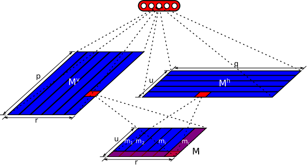
As a side effect of having multiple vectors to represent a sentence, the matrix sentence embedding is usually several times larger than vector sentence embeddings. This results in needing more parameters in the subsequent fully connected layer, which connects every hidden units to every units in the matrix sentence embedding. Actually in the example shown in Figure 1, this fully connected layer takes around 90% percent of the parameters. See Table 4. In this appendix we are going to introduce a weight pruning method which, by utilizing the 2D structure of matrix embedding, is able to drastically reduce the number of parameters in the fully connected hidden layer.
Inheriting the notation used in the main paper, let the matrix embedding has a shape of by , and let the fully connected hidden layer has units. The normal fully connected hidden layer will require each hidden unit to be connected to every unit in the matrix embedding, as shown in Figure 1. This ends up with parameters in total.
However there are 2-D structures in the matrix embedding, which we should make use of. Each row ( in Figure 1) in the matrix is computed from a weighted sum of LSTM hidden states, which means they share some similarities
| Hidden layer | Softmax | Other Parts | Total | Accuracy | |
|---|---|---|---|---|---|
| Yelp, Original, =3000 | 54M | 15K | 1.3M | 55.3M | 64.21% |
| Yelp, Pruned, =150, =10 | 2.7M | 52.5K | 1.3M | 4.1M | 63.86% |
| Age, Original, =4000 | 72M | 20K | 1.3M | 73.2M | 80.45% |
| Age, Pruned, =25, =20 | 822K | 63.75K | 1.3M | 2.1M | 77.32% |
| SNLI, Original, =4000 | 72M | 12K | 22.9M | 95.0M | 84.43% |
| SNLI, Pruned, =300, =10 | 5.6M | 45K | 22.9M | 28.6M | 83.16% |
To reflect these similarity in the fully connected layer, we split the hidden states into equally sized groups, with each group having units. The -th group is only fully connected to the -th row in the matrix representation. All connections that connects the -th group hidden units to other rows of the matrix are pruned away. In this way, Simillarity between different rows of matrix embedding are reflected as symmetry of connecting type in the hidden layer. As a result, the hidden layer can be interperated as also having a 2-D structute, with the number () and size () of groups as its two dimensions (The in Figure 6). When the total number of hidden units are the same (i.e., ), this process prunes away of weight values, which is a fairly large portion when is large.
On the other dimension, another form of similarity exists too. For each vector representation in , the -th element is a weighted sum of an LSTM hidden unit at different time steps. And for a certain -th element in all vector representations, they are summed up from a same LSTM hidden unit. We can also reflect this similarity into the symmetry of weight connections by using the same pruning method we did above. Thus we will have another 2-D structured hidden states sized -by-, noted as in Figure 6.
Table 4 takes the model we use for yelp dataset as a concrete example, and compared the number of parameters in each part of the model, both before and after pruning. We can see the above pruning method drastically reduces the model size. Note that the and in this structure can be adjusted freely as hyperparameters. Also, we can continue the corresponding pruning process on top of and over and over again, and end up with having a stack of structured hidden layers, just like stacking fully connected layers.
The subsequent softmax layer will be fully connected to both and , i.e., each unit in the softmax layer is connected to all units in and . This is not a problem since the speed of softmax is largely dependent of the number of softmax units, which is not changed.In addition, for applications like sentiment analysis and textural entailment, the softmax layer is so tiny that only contains several units.
Experimental results in the three datasets has shown that, this pruning mechanism lowers performances a bit, but still allows all three models to perform comparable or better than other models compared in the paper.
Appendix B Detailed Structure of the Model for SNLI Dataset
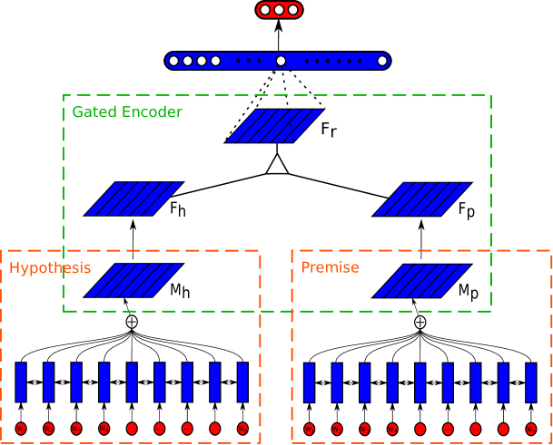
In Section 4.3 we tested our matrix sentence embedding model for the textual entailment task on the SNLI dataset. Different from the former two tasks, the textual entailment task consists of a pair of sentences as input. We propose to use a set of multiplicative interactions to combine the two matrix embeddings extracted for each sentence. The form of multiplicative interaction is inspired by Factored Gated Autoencoder (Memisevic, 2013).
The overall structure of our model for SNLI is dipicted in Figure 7. For both hypothesis and premise, we extract their embeddings ( and in the figure) independently, with a same LSTM and attention mechanism. The parameters of this part of model are shared (rectangles with dashed orange line in the figure).
Comparing the two matrix embeddings corresponds to the green dashed rectangle part in the figure, which computes a single matrix embedding () as the factor of semantic relation between the two sentences. To represent the relation between and , can be connected to and through a three-way multiplicative interaction. In a three-way multiplicative interaction, the value of anyone of , and is a function of the product of the others. This type of connection is originally introduced to extract relation between images (Memisevic, 2013). Since here we are just computing the factor of relations () from and , it corresponds to the encoder part in the Factored Gated Autoencoder in Memisevic (2013). We call it Gated Encoder in Figure 7.
First we multiply each row in the matrix embedding by a different weight matrix. Repeating it over all rows, corresponds to a batched dot product between a 2-D matrix and a 3-D weight tensor. Inheriting the name in (Memisevic, 2013), we call the resulting matrix as factor. Doing the batched dot for both hypothesis embedding and premise embedding, we have and , respectively.
| (10) |
| (11) |
Here and are the two weight tensors for hypothesis embedding and premise embedding.
The factor of the relation () is just an element-wise product of and (the triangle in the middle of Figure 7):
| (12) |
Here stands for element-wise product. After the layer, we then use an MLP with softmax output to classify the relation into different categlories.